Island Partition of Distribution System with Distributed Generators Considering Protection of Vulnerable Nodes

1
School of Electrical and Electronic Engineering, North China Electric Power University, Beijing 102206, China
2
Beijing Key Laboratory of Distribution Transformer Energy-Saving Technology, China Electric Power Research Institute, Beijing 100192, China
*
Authors to whom correspondence should be addressed.
Appl. Sci. 2017, 7(10), 1057; https://doi.org/10.3390/app7101057
Submission received: 5 September 2017
/
Accepted: 12 October 2017
/
Published: 16 October 2017
(This article belongs to the Special Issue Distribution Power Systems)
Abstract
:To improve the reliability of power supply in the case of the fault of distribution system with multiple distributed generators (DGs) and reduce the influence of node voltage fluctuation on the stability of distribution system operation in power restoration, this paper proposes an island partition strategy of the distribution system considering the protection of vulnerable nodes. First of all, the electrical coupling coefficient of neighboring nodes is put forward according to distribution system topology and equivalent electrical impedance, and the power-dependence relationship between neighboring nodes is calculated based on the direction and level of the power flow between nodes. Then, the bidirectional transmission of the coupling features of neighboring nodes is realized through the modified PageRank algorithm, thus identifying the vulnerable nodes that have a large influence on the stability of distribution system operation. Next, combining the index of node vulnerability, an island partition model is constructed with the restoration of important loads as the primary goal. In addition, the mutually exclusive firefly algorithm (MEFA) is also proposed to realize the interaction of learning and competition among fireflies, thus enhancing the globally optimal solution search ability of the algorithm proposed. The proposed island partition method is verified with a Pacific Gas and Electric Company (PG and E) 60-node test system. Comparison with other methods demonstrates that the new method is feasible for the distribution system with multiple types of distributed generations and valid to enhance the stability and safety of the grid with a relatively power restoration ratio.
1. Introduction
With the increasing connection of distributed generators (DGs), the distribution system operation mode has witnessed some major changes in terms of the control mode when compared with traditional distribution systems [1,2]. Due to its flexible operation mode, environmental friendliness, and high efficiency, DGs have effectively uplifted the efficiency of intelligent distribution system operation. Through the strategy of collaboratively controlling multiple DGs, the uninterrupted power supply of the distribution system can be ensured in the case of operation instability or fault, hence, helping realize the “self-healing” function of the distribution system [3].
To further promote the development of distribution system with multiple DGs, the Institute of Electrical and Electronic Engineers (IEEE) compiled the IEEE Std. 1547-2003 in 2003, encouraging the realization of island operation in multiple regions under fault through technical means [4]. In the modified standard IEEE 1547.4-2011, the definition of a microgrid was expanded to the distribution system with a relatively high penetration of DGs, believing that a future intelligent distribution system could be regarded as consisting of multiple microgrids with a collaborative control function [5]. The formulation of these standards indicates that when there is a fault in the future intelligent distribution system, island partition can be conducted according to an island zone partition or real-time operation status of the distribution system, so as to form multiple independently-running microgrid systems, realizing the autonomous operation of many islands in zones without fault, and ultimately ensure power supply stability and reliability.
Experts at home and abroad have conducted in-depth research on island partitioning of distribution systems with multiple distributed generators. Lasseter et al. [6] through assessing the operational status of DGs and the load in the case of a fault, proposed one type of self-adapting island partition strategy. Considering the DG capacity and distribution, Mao et al. [7] transformed the island partition into a finite tree issue in graph theory. Jikeng et al. [8] divided the island partition into two stages by constructing an initial island through the tree knapsack problem (TKP) method and then analyzed the generation and load status in the initial island, hence, realizing quadratic optimization. With a distribution system of microgrids as the research subject, Jingxiang et al. [9] proposed an energy risk evaluation-based island partition strategy considering the power supply and demand balance. With maximal power supply capacity and minimal energy consumption as target functions, El-Zonkoly et al. [10] established an island partition with load system operation constraint conditions by constructing a comprehensive learning particles swarm optimization (CLPSO). Pahwa et al. [11] proposed fast greedy algorithm (FGA) and bloom algorithm, respectively, for island issues in small-scale and large-scale distribution systems, which uplifted the computational efficiency of the island partition algorithm under different distribution systems. Zhang et al. [12] proposed one type of preliminary island partition method in the distribution system under a short-term power constraint mechanism, and verified the validity of the algorithm in PG and E 69 and IEEE 118 node systems. With a distribution system with multi-point faults as the research subject, Golari et al. [13] proposed one type of multi-stage stochastic programming model with minimal loss of load so as to realize the effective response of island partitioning against the power supply fault of the distribution system. The above references all used minimal island operation cost or maximal power supply capacity under a stable operational status as the target function for the solution of island partitioning and the optimization of solution efficiency. However, island partitioning normally occurs in the case of a distribution system fault accompanied by transient fluctuation. If timely fault isolation and protection are not taken for vulnerable nodes in the distribution system, it can cause fault expansion or relay protection, leading to further power loss of the remaining load nodes therein.
To further ensure the operation stability of the distribution system after island partitioning while realizing maximal power supply capacity, a vulnerable node protection-based island partition strategy of the distribution system with multiple distributed generators was proposed. Firstly, the electrical coupling relationship between distribution system nodes was analyzed to propose a vulnerable node identification method based on the electrical coupling transmission of neighboring nodes. According to load importance grading, the distribution system island partition mathematical model where important loads are restored in priority and its constraint conditions were established. Multi-agent theory was adopted to optimize the firefly algorithm to realize the learning and competition within the solution space and ultimately uplift the global optimization search ability of the algorithm. Ultimately, through simulation, the feasibility and validity of vulnerable node identification and the island partition method was verified.
2. Vulnerable Node Identification
A vulnerable node refers to the node whose transient stability has a relatively strong coupling with the operational stability of the distribution system. That is to say, when a vulnerable node experiences a transient fluctuation due to a fault, it will propagate to other nodes along the route through the distribution line and, thus, cause larger fluctuation amplitude and scope than a fault at non-vulnerable nodes. In a normal complex network theory, the distance between two nodes reflects the difficulty of flow transmission from one node to another node. According to [14,15], the distance in a power grid should be considered as the electrical distance in terms of equivalent impedance Zij:
where Uij is the voltage between nodes; Ii is the unit current of injection node i. The value of electrical equivalent impedance is equal to the voltage between nodes i and j after injecting unit current into the node i. For Ii = 1, Equation (1) can be converted into:
According to electrical network theory, the node impedance matrix containing J nodes can be expressed as:
Assume that the unit current only flows through nodes i and j in measuring electrical equivalent impedance, then Equation (3) can be rewritten into:
where and are, respectively, node voltages to ground; is the mutual impedance; and are the self-impedances of the nodes. is the measurement value.
According to Equation (4), Equation (2) can be further rewritten into:
where = , reflects the difficulty of the fault at node being transmitted to when current flows from node to . Due to that transient coupling of non-neighboring nodes needs to consider the reaction of the nodes on transmission route to transient fluctuation, nodes and herein specifically refer to neighboring ones.
The equivalent electrical impedance reflects the difficulty of node affecting the operation state of node . Inspired by Bompard et al. [14], we defined , the electrical coupling coefficient, to express the state correlation between node and .
where reflects how much node affects a single neighbor node when it fails. Therefore, we defined , the regional electric coupling coefficient (RECE), as the electrical coupling efficiency of node that reflects the ability of to affect all its neighboring nodes.
where Ωi is the neighboring node set of node i.
When a transient fluctuation or failure occurs in one node, the operational states of all nodes in the power system are influenced through the power transmission line, not only the neighboring nodes. In general, the node that is strongly coupled to the other nodes will have a wider and deeper influence on the power system when compared to a node that is weakly coupled to the other nodes. We regard these nodes as the vulnerable nodes.
As shown in Figure 1, nodes in a power system are electrically coupled to their neighbor nodes, forming several coupling regions. Due to the dynamic feature of mutual state coupling among regions and the nodes in the regions, the level of electrical coupling coefficient of the node belonging to different regions will change with a change in the electrical coupling coefficient of its neighboring nodes. For example, the RECE value of node v2 is first calculated based on the values of nodes v1 and v3. As their regional electrical coupling state are dynamic correlated to each other, the RECE value of node v2 will change according to its neighboring nodes and finally reach a balanced state. Thus, when we evaluate the RECE values of nodes that reflect the electrical coupling level between nodes and the power system, the dynamic state coupling process should be taken into account necessarily.
After further considering the dynamic coupling of nodes on fault propagation route, as well as the power-dependence relationship between neighboring nodes, we adopted a modified PageRank, called the coupling tracking rank algorithm (CT Rank), to conduct the bidirectional propagation of electrical coupling features of neighboring nodes so as to identify the influence of individual node fault upon system:
where is the neighboring node set of output current at absorption point, and is the set of neighboring nodes that make current output to node . is the apparent power that node supplies to node , . is the apparent power that node absorbs from node , . , are the active power and reactive power in the power transmission line. is the damping coefficient with [16].
The modified PageRank algorithm, with the neighboring electrical coupling coefficient Ci of the node as an initial value and the power supply and demand relationship between nodes as the coupling efficiency, seeks the transient coupling between nodes and the grid through an iterative loop so as to obtain the vulnerability index of node CTi, ultimately identifying the vulnerable nodes that have a large influence upon the operation stability of the distribution system.
3. Optimal Island Partition Strategy
3.1. Island Partition Model
The goal of island operation lies in maximizing the power supply capacity of the distribution system, isolating vulnerable nodes for protection, and reducing a secondary fault caused by the transient fluctuation of vulnerable nodes upon power supply restoration in the case of a fault of the distribution system. In ensuring the power supply, the loads of different grades have different influences upon personal safety and economic damage, so it is necessary to grade the load of the distribution system to ensure the supply reliability of important loads in priority and lower the influence of blackout upon social activities. According to constraints, like generator operation condition, power supply and demand balance, and controllable load proportion when the distribution system with multiple distributed generators operates in multiple islands, the island partition model is constructed as follows:
s.t.:
where , , are primary, secondary, and tertiary load weights, respectively; , , are primary, secondary, and tertiary load sets; is the vulnerability index of node ; and is the load active power of node . Due to the different types of loads, the load nodes can be divided into two categories: an uncontrollable load set () and a controllable load set (). is a variable that defines the connection state of a load. When the load node is uncontrollable, i.e., , can only equal zero or one, means the uncontrollable load node is disconnected to any island, and means the uncontrollable load is connected to some island. For a controllable load node, i.e., , the value of , which dependents to how much load is restored, is alterable. Assuming that node is on the route () connecting node and node , and node is a generator belonging to the node set in the island. Constraint (9c) ensures that there is always a route connecting to the generators inside the island for any load node therein, namely the connectivity constraint of the island node. is the power output value of the generation at node , and constraint (9d) ensures power supply and demand balance between the generator and the load after island partition. and represent the minimal and maximal values of the generation output power. Given that uncontrollable generators (PV, wind generator) cannot independently supply power for loads, constraint (9f) ensures that there is at least one controllable generation unit in any island. Considering the fluctuation and randomness of uncontrollable generators and loads after island partition, the power margin coefficient of controllable generators is set as in constraint (9g), to allow controllable generators to conduct real-time tracking compensation for power fluctuation in the island. is the output value of controllable generation at node , and is its maximal value of generation output power. Constraints (9h) and (9i) are, respectively, the branch voltage constraint and capacity constraint in an island. and are the minimal and maximal values of the branch voltage between nodes and . and are the minimal and maximal values for branch power transmission capacity.
According to [17], standby power in an island is the sum of 3% of the local load and 5% of the uncontrollable generator power:
where is the output power of the uncontrollable generators, . Equation (10) constrains the relationship between all generation unit power and load power at the time of island partition. Given that the right side is identically greater than, or equal to, 0, it also plays the role of ensuring power supply and demand balance within the island. Converting Equation (10) to obtain the power constraint of controllable generators:
Equation (11), in considering the dynamic changes of power for load and uncontrollable generation units within an island, ensures that there will be no insufficient power supply-caused transient fluctuations in the island operation through superposing the power gain coefficient before islanding the load and uncontrollable generators (making an increase of 3% in load power and a decrease of 5% in uncontrollable generation output as the ultimate state of system operation to calculate the minimal standby power margin for controllable generators).
In addition, because the operation mode of the distribution system with multiple distributed generators after island partitioning is similar to a microgrid, it can be considered to adopt a microgrid island operation generation control mode (such as V-f control) to realize the transient stability of loads within the island. Combining the above factors, equipment parameters, like line capacity, are not considered. Then the island partition model can be simplified as:
s.t.:
In Equation (12), the generation constraint conditions in Equation (9) are simplified through calculating the power supply and demand relationship between controllable generation, uncontrollable generation and load, as well as power margin conditions. Through further setting , it can be seen that . Therefore, while ensuring dynamic power balance in independent operation after island partitioning, constraint (12d) contains at least one controllable generation unit used for dynamically balancing the power supply and demand relationship.
3.2. Modified Firefly Algorithm
Firefly algorithm (FA) is one type of artificially bionic optimization search algorithm proposed by Yang et al. with Cambridge University in 2008 through imitating firefly attraction surrounding others with its own light [18,19]. In a FA optimization search, fireflies are initially randomly distributed into the solution space of the target function. The more superior the target function where the firefly is located, then the more attractive its luminance is to others. The influence of distance and the propagation medium should be considered in conducting the algorithm iteration, so as to obtain the solution for the target optimization function. The attractiveness between fireflies is in an inverse ratio with the distance and light intensity absorption coefficient, so the attractiveness between fireflies Xm and Xn can be defined as:
where refers to the maximal attractiveness between fireflies, which is related to the target function value of fireflies and ; refers to light intensity absorption coefficient, which is normally set to be as a constant; is the distance between fireflies and . In the iteration, if firefly is the most attractive object for firefly , then the position of firefly after movement for being attracted can be expressed as:
where α~N(0, 1) is the random step factor for satisfying normal distribution of 0–1, and K is the disturbance level.
To further improve the global optimization search ability of traditional FA, the mutually exclusive firefly algorithm (MEFA) was proposed with reference to the influence of territorial repulsion during courtship, to realize the interaction of learning and competition among fireflies. The set of male fireflies was assumed as and that of female ones was , then the mutually exclusive neighborhood of the former was . If two male fireflies enter into the mutually exclusive neighborhood in searching for optimization, then the disadvantaged one would escape along the diameter direction as shown in Figure 2. To quickly search the whole solution space, this paper also set the optimal firefly at the mutually exclusive neighborhood as male to avoid slipping into a local optimal solution too early.
Based on the above, the concrete steps of MEFA proposed in this paper are as follows:
Step 1: Randomly select firefly set , which is divided into a male firefly set and a female firefly set . Set the maximal absorption , mutually exclusive neighborhood radius , disturbance level , random step factor , convergence threshold , and iteration threshold .
Step 2: for female firefly , search for the most attractive firefly , and calculate the position of the female firefly after iteration:
Step 3: For the male firefly , search for the most attractive firefly , and calculate the position of male firefly after iteration:
Make a judgment whether the intersection between the mutually exclusive neighborhoods of the male firefly and the female firefly sets is empty or not. If and the objective function value of is more optimal, then the position of the male firefly is updated to:
Step 4: Make a judgment whether the convergence condition is met:
or determine if the iteration termination condition t ≥ T is met or not, then output the most optimal firefly; otherwise, search for whether the mutually exclusive neighborhood of the male firefly has a more optimal target value of the female firefly, then exchange the gender with the most optimal female firefly, and go back to Step 2.
4. Case Study
4.1. Test System Structure and Parameters
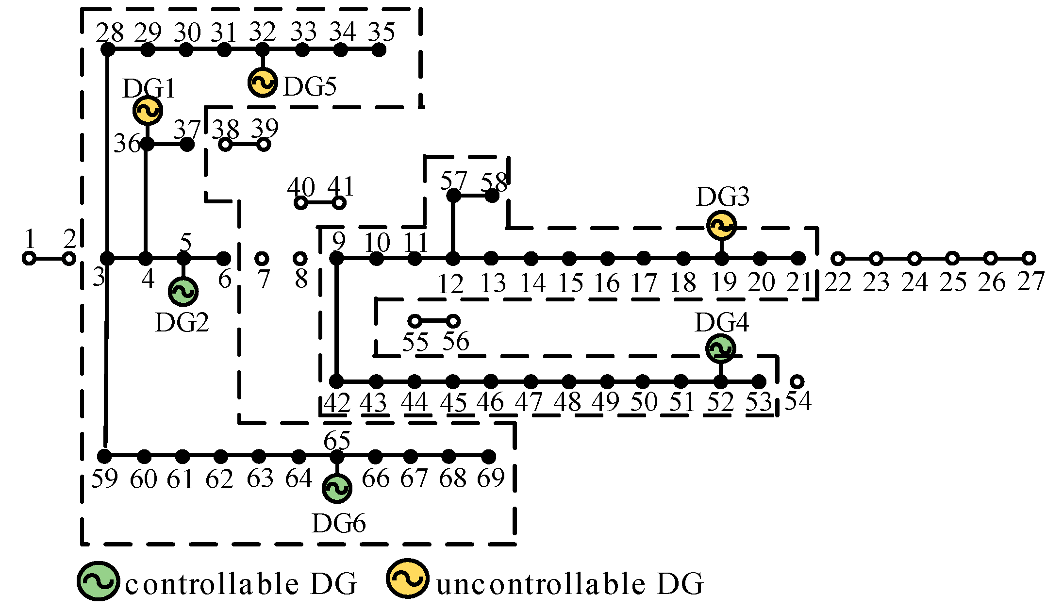
The American PG and E 69-node distribution system, as shown in Figure 3, was taken as the research subject, with an active load of 2802.19 kW and a voltage class of 12.66 kV. Reference [20] added three uncontrollable generators and three controllable generators (Table 1) into the system, with a maximal output power of 2470 kW and the load divided into primary, secondary, and tertiary grades (Table 2).
According to load controllability, it can be divided into completely controllable, partially controllable, and uncontrollable, as shown in Table 3.
4.2. Vulnerable Node Identification
In order to prove the validity of the proposed method for vulnerable node identification and obtain the system state when one node operation state changes, the three-phase fault was set to trigger a sudden operation state change of each node each time, and obtain the voltage fluctuation of the power grid. In each simulation, we just set the fault on one node for one time. Therefore, the test in PSCAD was simulated sixty-nine times, since there are sixty-nine nodes in a PG and E 69-node test system. In Appendix A, we also did the same test thirty-nine times, since there are thirty-nine nodes in an IEEE 39-node test system. Regarding the node which impacts the system operation state most as the vulnerable node, the vulnerability index of each node was added into the objective function Equation (9) to ensure the vulnerable nodes will be protected as much as possible when branch 2–3 is broken. A PG and E 69-node system, as shown in Figure 4, was taken as the experimental subject to build a simulation model in PSCAD, and the experiments of the three-phase ground fault were conducted for each node. Then, the voltage fluctuation levels of the nodes in the case of a fault are obtained, as shown in Figure 4.
From Figure 4, it can be seen that the voltage fluctuation level caused by three-phase node fault at different nodes varied, and there was a major difference in the influence of neighboring nodes upon transient operation stability of the power grid. Therefore, to verify the correctness of the proposed vulnerable node identification method, the vulnerability index and voltage fluctuation amplitude were correlated, hence obtaining the results shown in Figure 5.
Figure 5 is the scatter diagram of the correlation between the node vulnerability index and the voltage fluctuation amplitude caused by the node three-phase grounding fault, which was obtained using the proposed node vulnerability identification method. From Figure 5, it can be seen that the obtained node vulnerability index was basically positively correlated with the voltage fluctuation amplitude. Meanwhile, due to the differences in voltage fluctuation diffusion and maximal voltage fluctuation amplitude caused by node fault, although the average value of voltage fluctuation amplitude was close, there was still a difference in node vulnerability. For example, the vulnerability of the most vulnerable nodes 8 and 9 were, respectively, 0.3757 and 0.387, and the average voltage fluctuation in the case of a fault were, respectively, 0.0670 p.u. and 0.0676 p.u., with a maximal voltage fluctuation of 0.2554 p.u. and 0.2564 p.u. Hence, according to the assessment, node 9 was more vulnerable than node 8.
Appendix A is the simulation calculation of node vulnerability in an IEEE 39-node distribution system, hence, further verifying the validity of the proposed node vulnerability identification method.
4.3. Island Partition Verification
Branch 2–3 in the PG and E 69-node system was set to have a fault of the three-phase grounding, with the branch switch disconnected through fault isolation, leading to the failure of the power supply to node 3 and its downstream nodes through the public distribution system. The primary, secondary, and tertiary load weights were set to be , , , respectively [21]. The proposed algorithm, according to node vulnerability, position of distributed generators, and its capacity, was adopted to conduct island partition in the case of a fault of the distribution system with multiple distributed generators, as shown in Figure 6.
As shown in Figure 6, the distribution system with multiple distributed generators was divided into two islands for independent operation after a fault, with a total load restoration rate of 62.04%. Among them, the restoration rate was 100% for primary loads, 59.23% for secondary loads, and 47.04% for tertiary loads. Specifically, for island-2 of Figure 6, all the primary loads and uncontrollable loads in the power transmission line are restored at the first stage. In this period, only controllable non-primary loads (secondary loads and tertiary loads) are waiting to be selected to be restored. To restore the secondary loads most, all the controllable tertiary load nodes in island-2 of Figure 6 are not fully restored and the controllable secondary load is partly restored according to the remaining power supply ability of DGs at the same time. In this case, there are still some controllable secondary load nodes are not under a fully-restored state. In other words, the DGs in island-2 of Figure 6 have already supplied their maximum power to the loads. Thus, it is meaningless to put node 53 into island-2, and node 53 may be under a no-power state even if it is connected to island-2.
In addition, in order to ensure dynamic power balance in each island’s independent operation after island partition, the standby power in one island should be the sum of 3% of the local load and 5% of uncontrollable generator power. Therefore, some controllable generators are not at maximum power for balancing the power fluctuation from the local load and the uncontrollable generators. Detailed load restoration and power output is shown in Table 4 and Table 5.
The island partition scheme in this paper was compared with the algorithm proposed in [8,22], and their island partition schemes were obtained as shown in Figure 7 and Figure 8.
The load restoration amount and rate of three methods are as shown in Table 6.
Table 6 presents the statistical results of load restoration after island partition through the three methods. Reference [8] divided the distribution system into four islands for independent operation; but due to the calculation not considering that uncontrollable units, like photovoltaics and wind power, cannot independently supply power to the local load, it could not form stable and effective islands. Therefore, the statistics abandoned the load contained by ineffective islands so as to obtain a total load restoration rate of 53.44% in [8]. Both the method in this paper and [22] combined uncontrollable and controllable power generators, prescribing that every island should contain at least one controllable power unit and dividing the distribution system into two effective islands for independent power supply. According to Table 6, the total load restoration of the method proposed in this paper was close to the method in [22], being 62.04% and 62.55%, respectively.
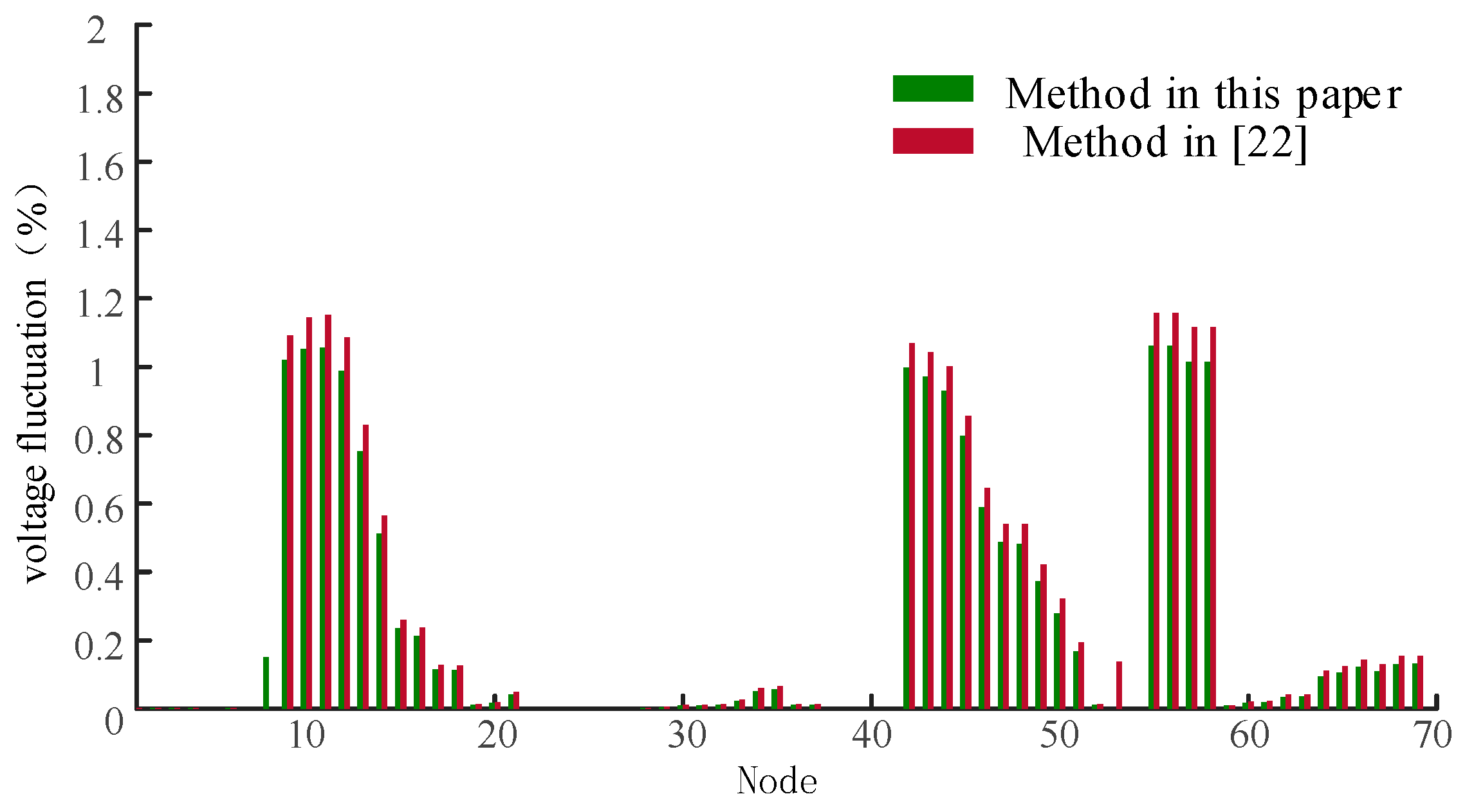
After the fault of branch 2–3 is fixed, the distribution system should close all the brakes which were open before for power restoration. During this power restore process, the voltage of the power grid will fluctuate, caused by the sudden change of load power and the switch of brakes. Therefore, two kinds of island partition were set in PSCAD. Assuming that branch 2–3 is fixed, the power restoration is, respectively, executed under two different island partition configurations. In PSCAD, a power supply restoration experiment was conducted on the island scheme of this paper and that of [22], obtaining the absolute percentage of voltage fluctuation at various nodes in the distribution system, as shown in Figure 9, but the voltage fluctuation of nodes without power supply in island operation was not included in the statistics.
From Figure 9 and Table 7, it can be seen that the maximal voltage fluctuation and average voltage fluctuation produced using the island scheme proposed in this paper at the time of power supply restoration were both lower than those produced using the scheme in [22]. Therefore, the island scheme in this paper, while ensuring a relatively high power supply restoration rate, has effectively lowered the transient fluctuation of normally running nodes at the time of power supply restoration and uplifted the stability of the distribution system in terms of power supply. In other words, if there is a large voltage fluctuation during the power restoration process, it may cause the power grid to operate at an unstable point. Furthermore, if the protection devices are triggered by this voltage fluctuation, the outage may happen again. Thus, we conclude that the proposed island partition method can enhance the stability and safety of the power grid during the power restoration process effectively.
5. Conclusions
Aiming at the issue of island partitioning of a distribution system with multiple distributed generators, most of the existing studies fail to consider the influence of island partition results on system stability in later power restoration. Therefore, this paper constructs an island partition method considering the protection of vulnerable nodes and mainly focuses on two points: (1) identifying the vulnerable nodes in distribution system, which will impact the stability of the grid most; and (2) designing the island partition strategy considering the protection of both the primary load and vulnerable node. To identify the vulnerable nodes in the distribution system, we proposed a coupling feature analysis method of neighboring nodes. Additionally, we also established a kind of modified PageRank algorithm to realize the bidirectional transmission of coupling features to calculate the transient coupling between individual nodes and other nodes in the distribution system. Thus, the vulnerable node which has the ability of impacting the stability of the power grid the most is identified. Then, we construct an island partition model and its constraints with important load restoration and vulnerable node protection taken as its objectives, and propose the mutually exclusive firefly algorithm to uplift its ability to search for the island partition’s globally optimal solution. The simulation results show that the operation state of the distribution system during the power restoration process is stable. Thus, we conclude that the method proposed in this paper can effectively enhance the stability and safety of the distribution system during the power restoration process with a relatively high ratio of power supply for important loads and provide references for grid dispatchers and controllers in terms of power grid emergency control.
Acknowledgements
This work was supported by Beijing Municipal Natural Science Foundation (Approaches on Interdependent Distribution System Reconfiguration Based on Key Node Protection) and the National High Technology Research and Development of China (2015AA050203).
Author Contributions
Xu Gang provided theoretical guidance. Wu Shunyu designed the algorithm for vulnerable nodes identification and did the simulations of island partition. Tan Yuanpeng optimized the algorithm of island partition.
Conflicts of Interest
The authors declare no conflict of interest.
Appendix A
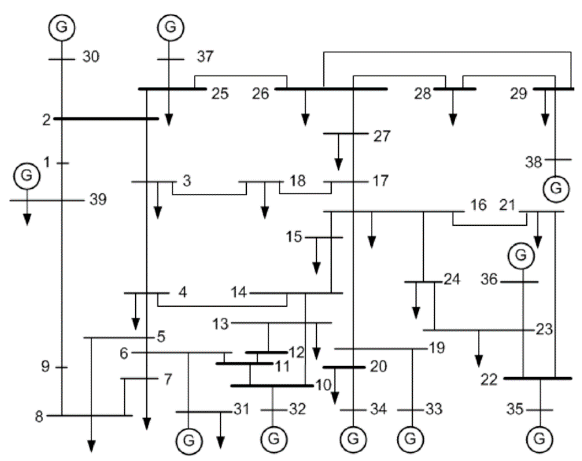
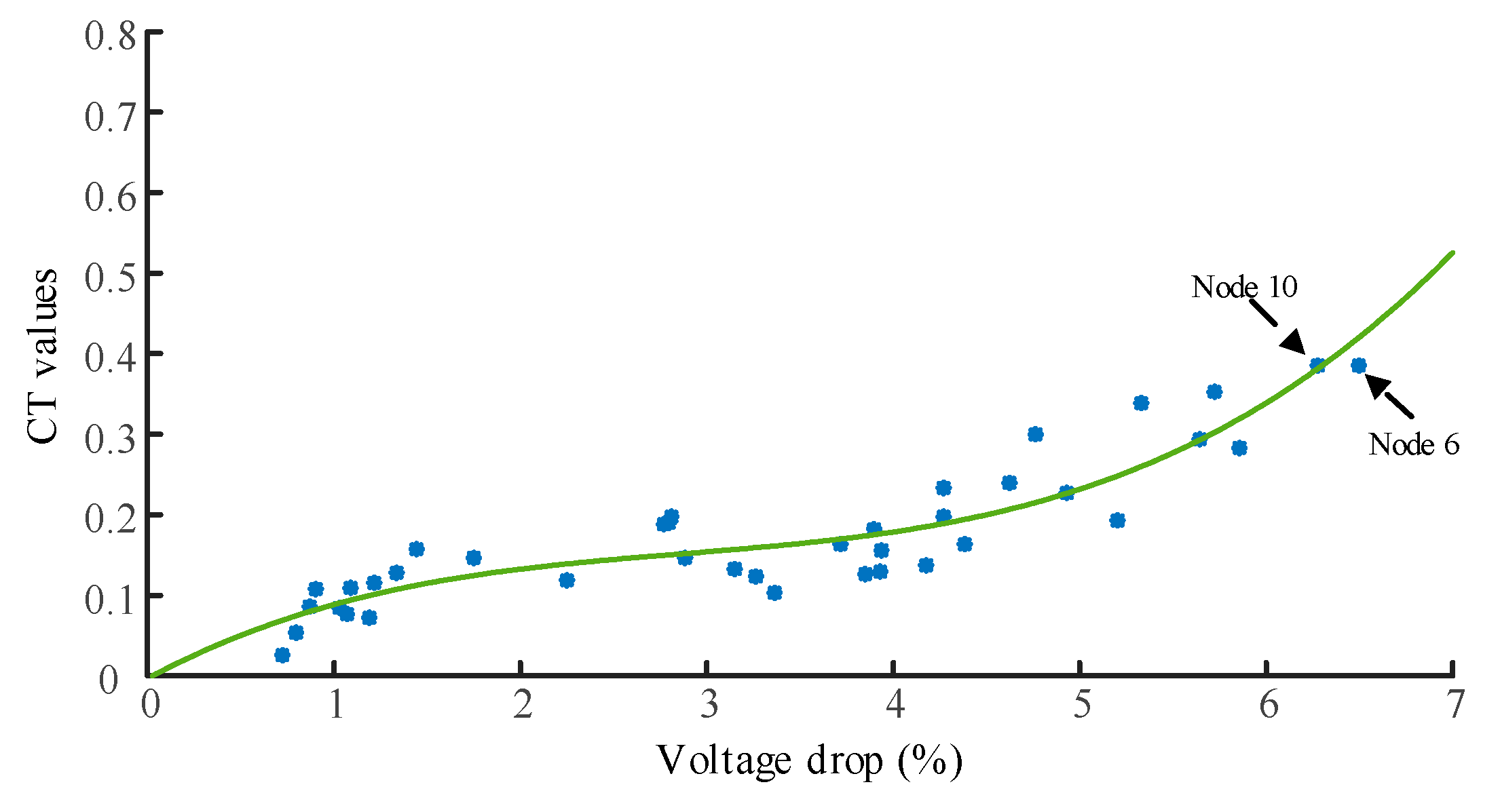
In PSCAD, an IEEE 10 39-node system was built, as shown in Figure A1, to conduct the experiment of a three-phase grounding short circuit on nodes and calculate their vulnerability, by which the correlation scatter diagram between node vulnerability and system voltage fluctuation was obtained, as shown in Figure A2.
Figure A1.
IEEE 39-BUS test system.
As shown in Figure A2, the proposed node vulnerability evaluation method could effectively correlate node vulnerability and operation stability of the distribution system, and identify the vulnerable nodes that had major influence upon operation stability of the distribution system.
Figure A2.
Node CT values and system voltage drop.

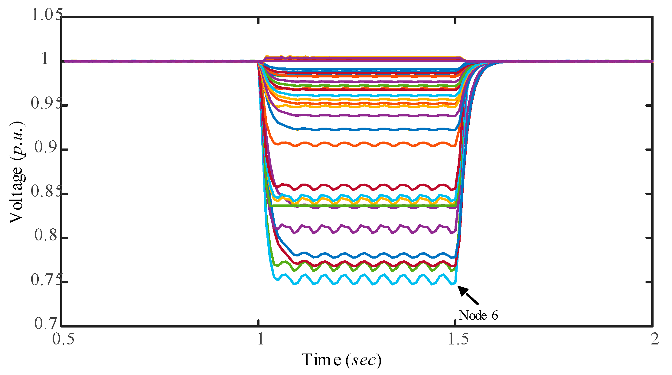
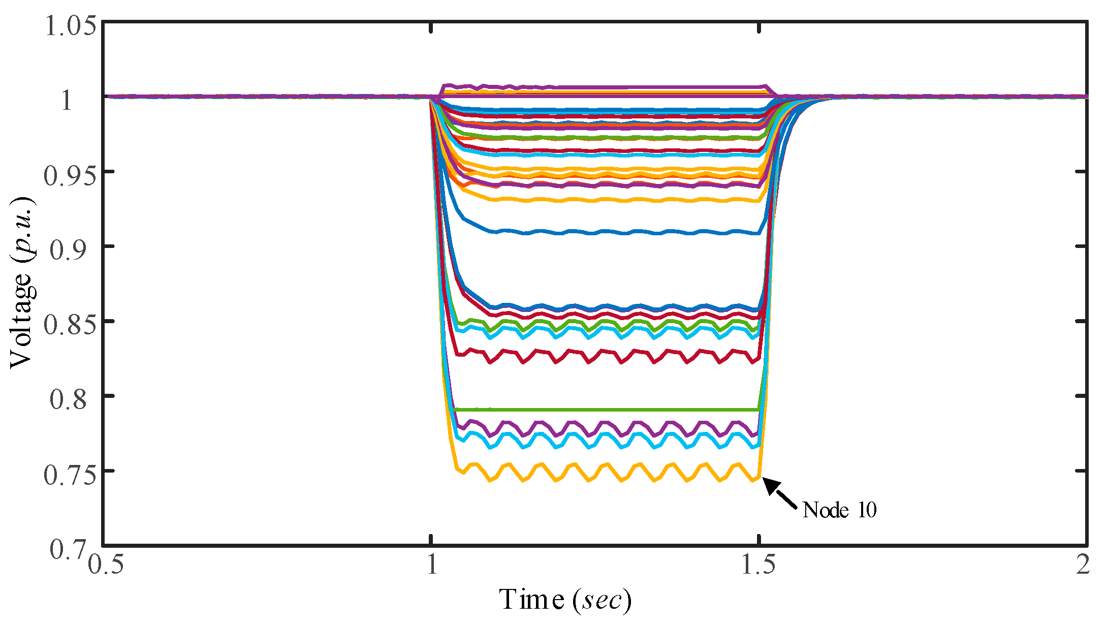
Figure A3 and Figure A4 show the voltage fluctuations of other nodes when nodes 6 and 10 have faults. When there was a three-phase short circuit grounding fault in node 6 and 10, the maximal voltage decrease caused thereby was 0.242 p.u. and 0.246 p.u. respectively, and there were more nodes with voltage fluctuations caused by the fault at node 10. Hence, although the average voltage decrease of the distribution system during the fault at node 6 was larger, node vulnerability CT6 ≈ CT10 due to the wider influence of node 10.
Figure A3.
Voltage drop curve of nodes when node 6 fails.

Figure A4.
Voltage drop curve of nodes when node 10 fails.

References
- Al Abri, R.S.; El-Saadany, E.F.; Atwa, Y.M. Optimal placement and sizing method to improve the voltage stability margin in a distribution system using distributed generation. IEEE Trans. Power Syst. 2013, 28, 326–334. [Google Scholar] [CrossRef]
- Guan, W.; Tan, Y.; Zhang, H.; Song, J. Distribution system feeder reconfiguration considering different model of DG sources. Int. J. Electr. Power Energy Syst. 2015, 68, 210–221. [Google Scholar] [CrossRef]
- Wang, Z.; Chen, B.; Wang, J.; Chen, C. Networked microgrids for self-healing power systems. IEEE Trans. Smart Grid 2016, 7, 310–319. [Google Scholar] [CrossRef]
- IEEE Standard 1547. IEEE Standard for Interconnecting Distributed Resources with Electric Power Systems. 2003. Available online: https://standards.ieee.org/findstds/standard/1547-2003.html (accessed on 29 September 2016).
- Lasseter, R.H. Smart distribution: Coupled microgrids. Proc. IEEE 2011, 99, 1074–1082. [Google Scholar] [CrossRef]
- Caldon, R.; Stocco, A.; Turri, R. Feasibility of adaptive intentional islanding operation of electric utility systems with distributed generation. Electr. Power Syst. Res. 2008, 78, 2017–2023. [Google Scholar] [CrossRef]
- Mao, Y.; Miu, K.N. Switch placement to improve system reliability for radial distribution systems with distributed generation. IEEE Trans. Power Syst. 2003, 18, 1346–1352. [Google Scholar]
- Lin, J.; Wang, X.; Wu, P.; Liu, S.; Shao, G.; Ma, X.; Xu, X.; Luo, S. Two-stage method for optimal island partition of distribution system with distributed generations. IET Gener. Transm. Distrib. 2012, 6, 218–225. [Google Scholar]
- Zhao, J.; Niu, H.; Zhang, X. Island partition of distribution network with microgrid based on the energy at risk. IET Gener. Transm. Distrib. 2017, 11, 830–837. [Google Scholar]
- El-Zonkoly, A.; Saad, M.; Khalil, R. New algorithm based on CLPSO for controlled islanding of distribution systems. Int. J. Electr. Power Energy Syst. 2013, 45, 391–403. [Google Scholar] [CrossRef]
- Pahwa, S.; Youssef, M.; Schumm, P.; Scoglioa, C.; Schulza, N. Optimal intentional islanding to enhance the robustness of power grid networks. Phys. A Stat. Mech. Appl. 2013, 392, 3741–3754. [Google Scholar] [CrossRef]
- Zhang, M.; Chen, J. Islanding and scheduling of power distribution systems with distributed generation. IEEE Trans. Power Syst. 2015, 30, 3120–3129. [Google Scholar] [CrossRef]
- Golari, M.; Fan, N.; Wang, J. Two-stage stochastic optimal islanding operations under severe multiple contingencies in power grids. Electr. Power Syst. Res. 2014, 114, 68–77. [Google Scholar] [CrossRef]
- Bompard, E.; Pons, E.; Wu, D. Analysis of the structural vulnerability of the interconnected power grid of continental Europe with the Integrated Power System and Unified Power System based on extended topological approach. Int. Trans. Electr. Energy Syst. 2013, 23, 620–637. [Google Scholar] [CrossRef]
- Bompard, E.; Napoli, R.; Xue, F. Analysis of structural vulnerabilities in power transmission grids. Int. J. Crit. Infrastruct. Prot. 2009, 2, 5–12. [Google Scholar] [CrossRef]
- Wu, X.; Kumar, V.; Quinlan, J.R.; Ghosh, J.; Yang, Q.; Motoda, H.; McLachlan, G.J.; Ng, A.; Liu, B.; Yu, P.S.; et al. Top 10 algorithms in data mining. Knowl. Inf. Syst. 2008, 14, 1–37. [Google Scholar] [CrossRef]
- Energy, G.E. Western Wind and Solar Integration Study; National Renewable Energy Laboratory: Golden, CO, USA, 2010. [Google Scholar]
- Gandomi, A.H.; Yang, X.S.; Talatahari, S.; Alavi, A.H. Firefly algorithm with chaos. Commun. Nonlinear Sci. Numeri. Simul. 2013, 18, 89–98. [Google Scholar] [CrossRef]
- Yang, X.S. Firefly algorithm, Levy flights and global optimization. In Research and Development in Intelligent Systems XXVI; Springer: London, UK, 2010; pp. 209–218. [Google Scholar]
- Baran, M.E.; Wu, F.F. Optimal capacitor placement on radial distribution systems. IEEE Trans. Power Deliv. 1989, 4, 725–734. [Google Scholar] [CrossRef]
- Wang, X.; Lin, J. Island Partition of the Distribution System with Distributed Generation Based on Branch and Bound Algorithm. Proc. CSEE 2011, 31, 16–20. [Google Scholar]
- Bing, L.; Jing, Z.; Peijie, L. Island partition of distribution network with unreliable distributed generators. Autom. Electr. Power Syst. 2015, 39, 59–65. [Google Scholar]
Figure 1.
Electrical coupling of multiple regions.
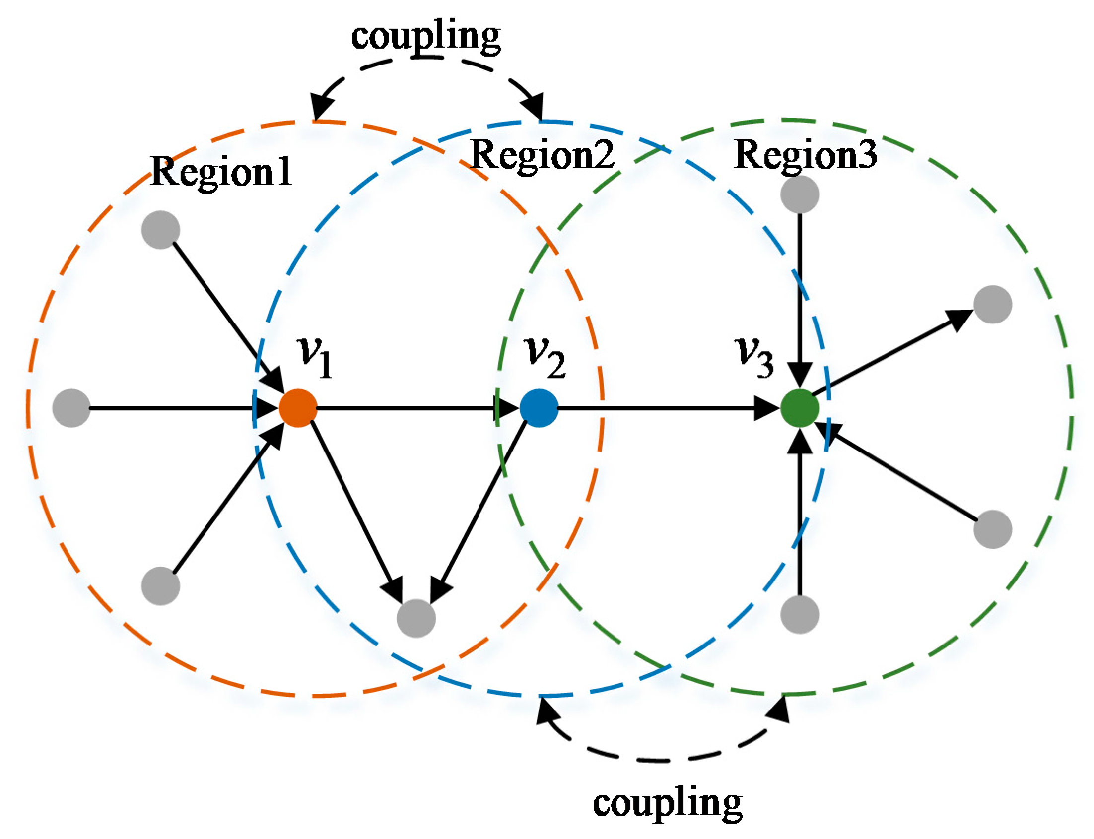
Figure 2.
Diagram of the mutually exclusive influence between fireflies.
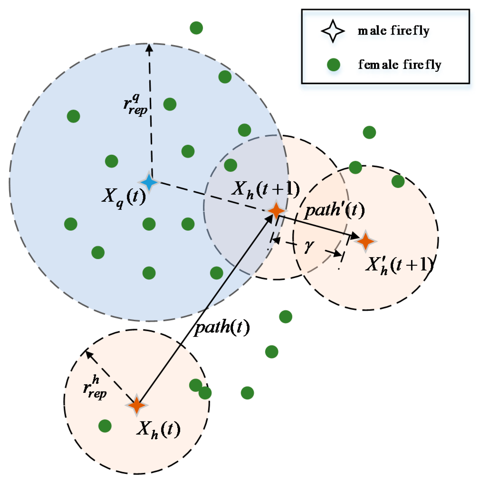
Figure 3.
Structure of a PG and E 69-node system.
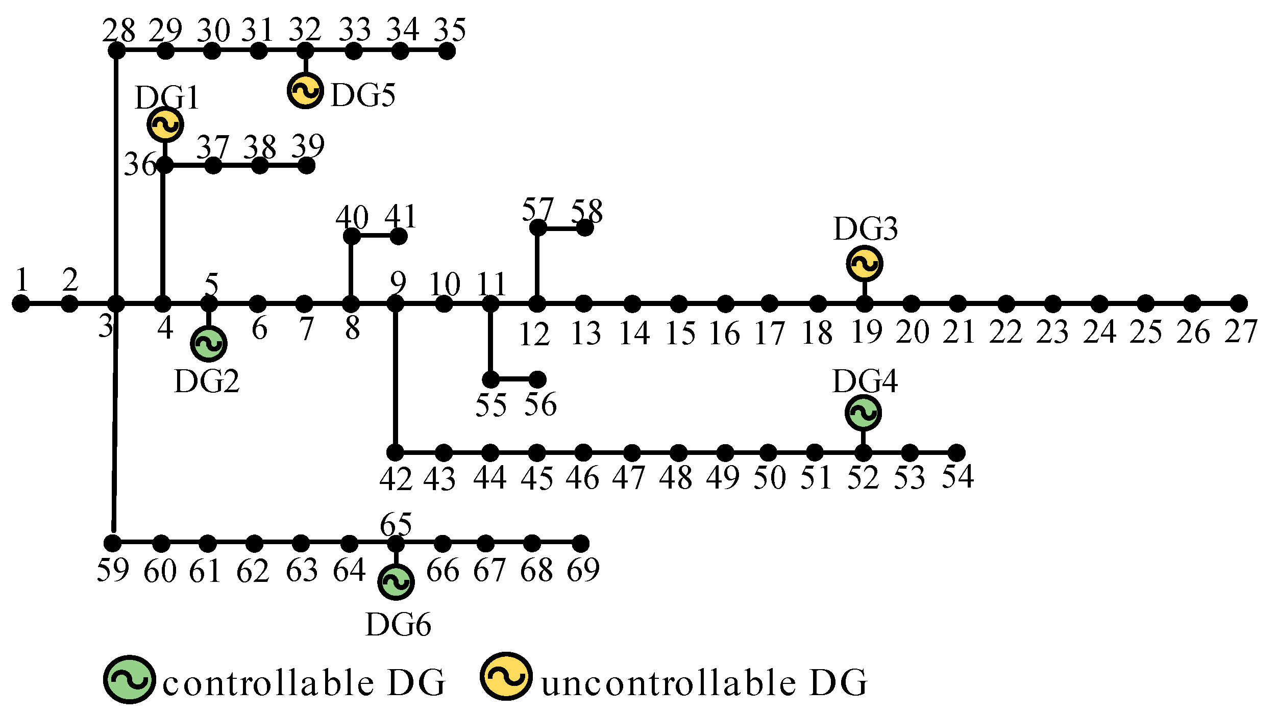
Figure 4.
Voltage fluctuation level of nodes in the distribution system during a fault.
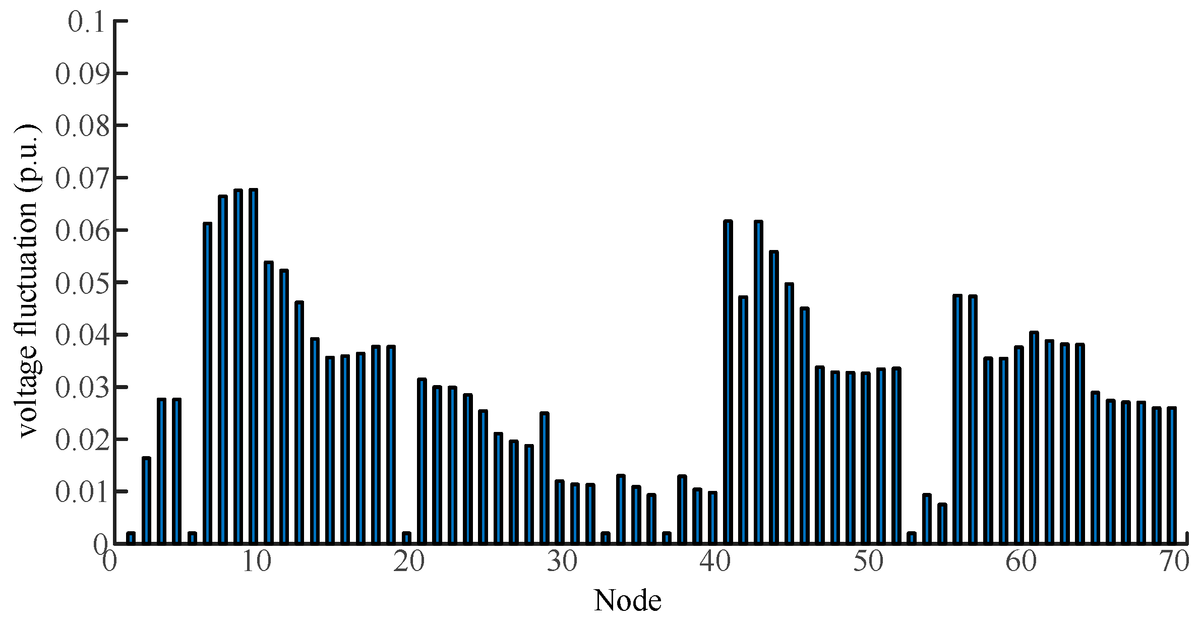
Figure 5.
Correlation scatter diagram between voltage fluctuation and node vulnerability.
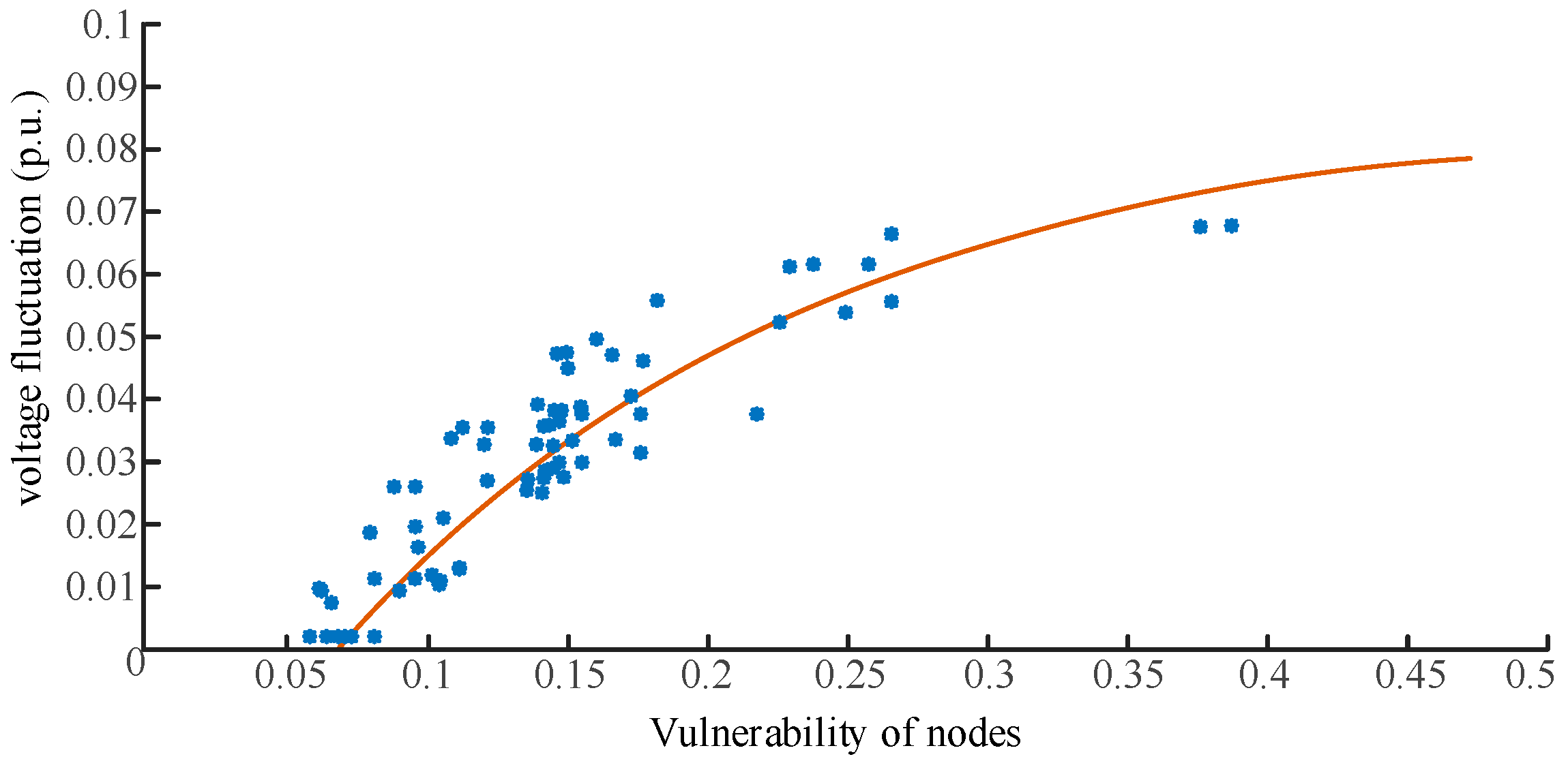
Figure 6.
Island partition scheme of the distribution system with multiple distributed generators.
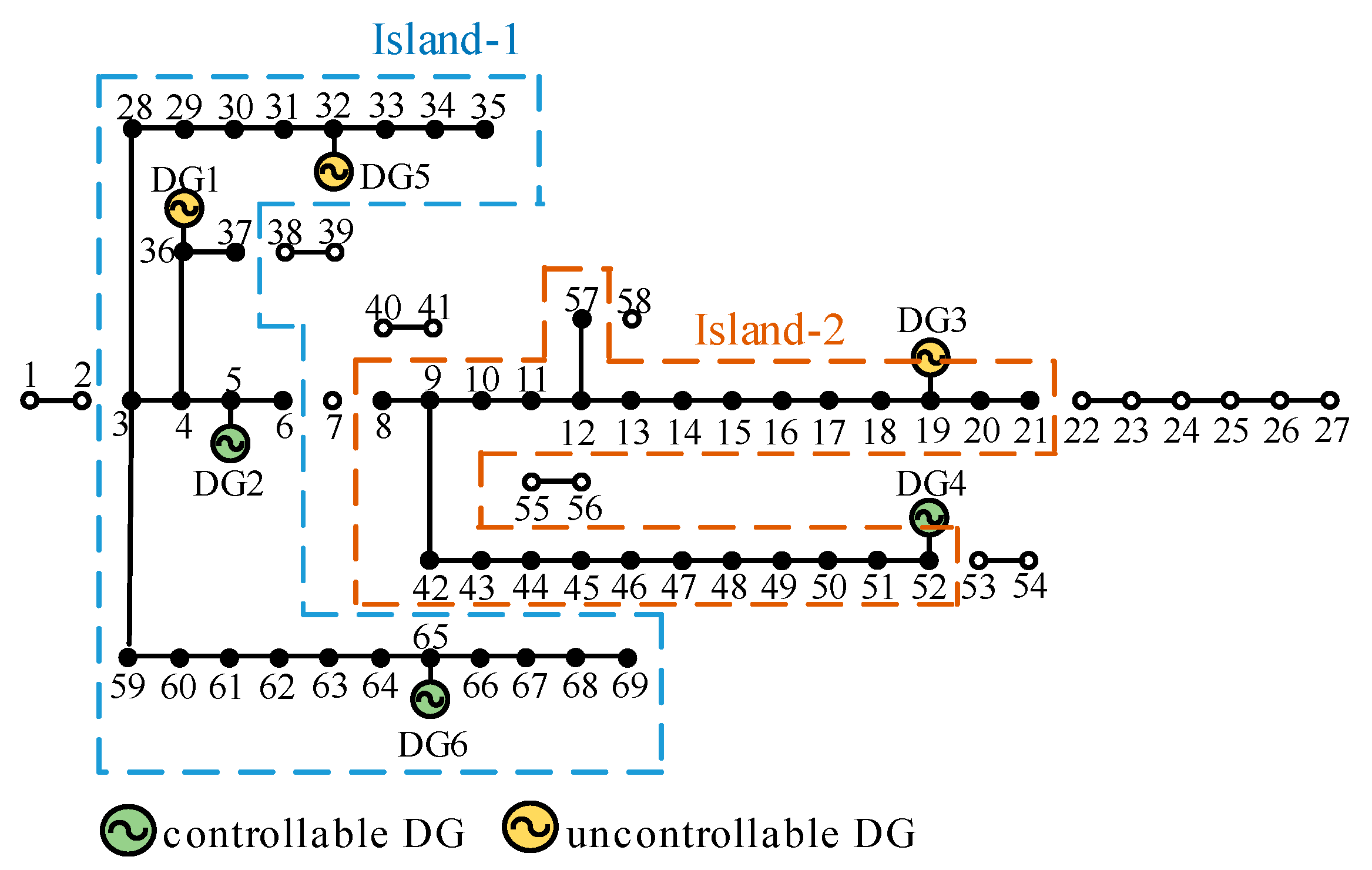
Figure 7.
Island partition formed by the method in [8].
Figure 7.
Island partition formed by the method in [8].
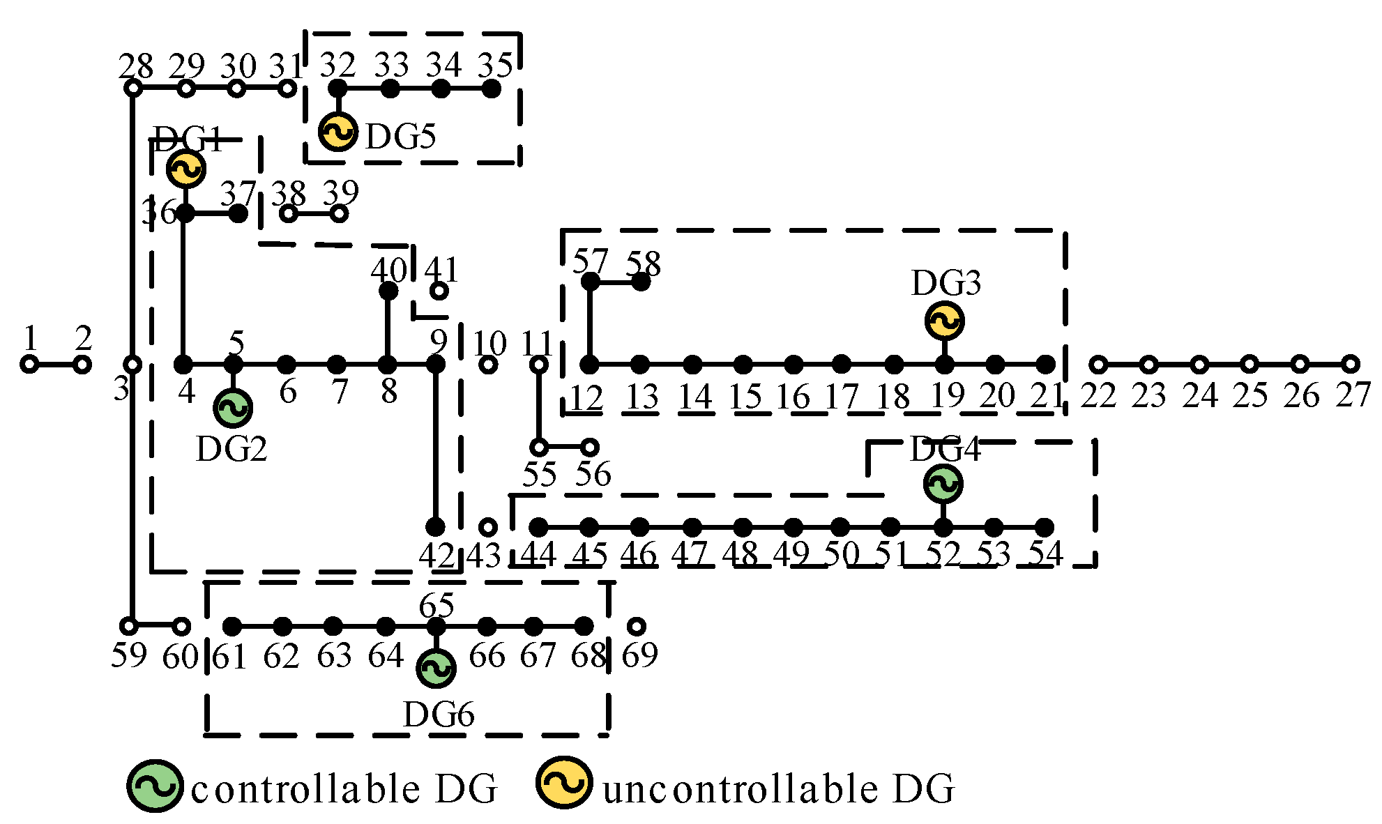
Figure 8.
Island partition formed by the method in [22].
Figure 8.
Island partition formed by the method in [22].

Figure 9.
Comparison of voltage fluctuations at power supply-restored nodes.

Table 1.
Parameters of DGs.
| DG | Node | DG Type | Max Power/kW | Effective Power/kW |
|---|---|---|---|---|
| DG1 | 36 | Uncontrollable | 50 | 47.5 |
| DG2 | 5 | Controllable | 200 | 200 |
| DG3 | 19 | Uncontrollable | 380 | 361 |
| DG4 | 52 | Controllable | 1700 | 1700 |
| DG5 | 32 | Uncontrollable | 40 | 38 |
| DG6 | 65 | Controllable | 100 | 100 |
Table 2.
Types of loads.
| Load Grade | Node No. |
|---|---|
| 1 | 6, 9, 12, 18, 35, 37, 42, 51, 57, 62 |
| 2 | Remaining nodes |
| 3 | 7, 10, 11, 13, 16, 22, 28, 43, 45–48, 59, 60, 63 |
Table 3.
Types of load controllability.
| Controllable Type | Load Node No. |
|---|---|
| Completely controllable | 13, 26, 27, 34, 35, 39–41, 43, 44, 48, 53–58, 66–69 |
| 40% Controllable | 11, 21, 38 |
| Uncontrollable | Remaining load nodes |
Table 4.
Load restoration information.
| Load Grade | Total Load/kW | Restored Load/kW | Restoration Rate/% | |
|---|---|---|---|---|
| Distribution system | 1 | 410.95 | 410.95 | 100 |
| 2 | 2890.64 | 1712.24 | 59.23 | |
| 3 | 500.6 | 235.5 | 47.04 | |
| Island 1 | 1 | 111.6 | 111.6 | 100 |
| 2 | 171.14 | 171.14 | 100 | |
| 3 | 76 | 76 | 100 | |
| Island 2 | 1 | 299.35 | 299.35 | 100 |
| 2 | 1554 | 1541.1 | 99.17 | |
| 3 | 352.9 | 160.5 | 45.48 | |
Table 5.
The power output of distributed generators.
| DG | Node | DG Type | Max Power /kW | Actual Output /kW |
|---|---|---|---|---|
| DG1 | 36 | Uncontrollable | 50 | 50 |
| DG2 | 5 | Controllable | 200 | 200 |
| DG3 | 19 | Uncontrollable | 380 | 380 |
| DG4 | 52 | Controllable | 1700 | 1639.95 |
| DG5 | 32 | Uncontrollable | 40 | 40 |
| DG6 | 65 | Controllable | 100 | 68.71 |
Table 6.
Comparison of island partition load restoration results.
| Scheme | Total Restoration/kW | Primary Load/kW | Secondary Load/kW | Tertiary Load/kW |
|---|---|---|---|---|
| Method in this paper | 2358.69 | 410.95 | 1712.24 | 235.5 |
| [8] | 2031.86 | 172.67 | 1694.07 | 165.12 |
| [22] | 2378.19 | 410.95 | 1817.74 | 149.5 |
Table 7.
Voltage fluctuation of distribution system upon power supply restoration.
| Scheme | Max Voltage Fluctuation/% | Average Voltage Fluctuation/% |
|---|---|---|
| Method in this paper | 1.06 | 0.29 |
| Method in [22] | 1.16 | 0.35 |
© 2017 by the authors. Licensee MDPI, Basel, Switzerland. This article is an open access article distributed under the terms and conditions of the Creative Commons Attribution (CC BY) license (http://creativecommons.org/licenses/by/4.0/).
Share and Cite
MDPI and ACS Style
Xu, G.; Wu, S.; Tan, Y. Island Partition of Distribution System with Distributed Generators Considering Protection of Vulnerable Nodes. Appl. Sci. 2017, 7, 1057. https://doi.org/10.3390/app7101057
AMA Style
Xu G, Wu S, Tan Y. Island Partition of Distribution System with Distributed Generators Considering Protection of Vulnerable Nodes. Applied Sciences. 2017; 7(10):1057. https://doi.org/10.3390/app7101057
Chicago/Turabian StyleXu, Gang, Shunyu Wu, and Yuanpeng Tan. 2017. "Island Partition of Distribution System with Distributed Generators Considering Protection of Vulnerable Nodes" Applied Sciences 7, no. 10: 1057. https://doi.org/10.3390/app7101057
Note that from the first issue of 2016, this journal uses article numbers instead of page numbers. See further details here.