Modeling of Temperature Field during Multi-Pass GMAW Surfacing or Rebuilding of Steel Elements Taking into Account the Heat of the Deposit Metal

Abstract

This paper proposed an analytical model for describing the temperature field of multi-pass arc weld surfacing. The temperature field is described analytically assuming a bimodal volumetric model of the heat source and a semi-infinite body model of the (rebuilt) workpiece. The suggested analytical solution takes into account the temperature changes caused not only by the direct heat of an electric arc, but also by the heat of the applied weld (melted metal of electrode). The solution considers temperature increments caused by overlaying consecutive welding sequences and by self-cooling of areas previously heated. Computations of the temperature field are carried out during the multi-pass gas metal arc welding (GMAW) surfacing of a steel plate. The results are presented in the form of transient and maximum (achieved in whole welding process) temperature distributions in the element’s cross-section, as well as thermal cycles at the selected point.

1. Introduction

In the case of multi-pass surfacing, the application of subsequent welds causes previous welds to heat up and melt. During subsequent thermal cycles, the material in a heat-affected zone can undergo multiple-phase transformations leading to the diversification of the structure between welds and the heat-affected zone, at the same surfacing parameters. It results in diversified states of strains and stresses in the heat-affected zone, as well as outside it.

Tracing changes in temperature allows one to determine the phase transformations and stress state. The knowledge of the distribution and the value of permanent deformations and internal stresses after welding is necessary due to their superposition with the strains and stresses generated during the welding process. The knowledge of thermo-mechanical state changes in the deposited steel elements is the basis for the rational design of these processes.

The modeling of the temperature field in welding processes is dominated by two approaches. The first—numerical—applies the finite difference method, elementary heat balance and finite element method (FEM). The second approach consists of analytical solutions, which most commonly use integral transformation methods and Green’s functions.

The literature on the calculation of the temperature field and the welding thermal cycles during single-welding is extensive. Modeling the temperature field during welding was initiated by works by Rosenthal [1] and Rykalin [2], who assumed point and linear models of the heat source, respectively. Eagar and Tsai [3] modified Rosenthal’s model including the two-dimensional (2D) Gaussian distributed heat source and developed a solution to the travelling heat source in a semi-infinite steel plate. Since the adoption of a point heat source located near the center of the weld results in significantly deviating from the actual temperature values, many researchers have tried to obtain the solution closest to the real temperature distribution, using different models of heat sources. The model of a double-ellipsoidal three-dimensional (3D) heat source was first introduced by Goldak et al. [4].

Na and Lee [5] used an annular heat source where the intensity of the heat flux within the center of the arc welding was determined according to the parameter defined as the radius at which the intensity of the arc power was 5% of the maximum intensity. Bo and Cho [6] derived an analytical solution for transient temperature field in finite thickness plate during single-pass arc welding, assuming Gaussian distribution of heat source. An analytical solution for temporary temperature field of fillet weld has been presented by Jeong and Cho [7] and wasapplied by Fassani and Trevisan [8] to compare the thermal cycles during multi-pass gas metal arc welding (GMAW) which was computed for Rosenthal’s models of point heat sources and one-dimensional (1D) Gaussian. The solution is presented in the form of temperature distribution perpendicular to the welding direction. On the other hand, the solution of the temperature field in a massive body caused by a half-elliptical double-ellipsoidal volumetric heat source has been presented by Nguyen et al. [9]. Kwon and Weckman [10] carried out the thermal analysis in double-sided arc welding of an aluminum alloy plate. Ghosh at al. [11] analyzed thermal behaviour during SAW (submerged arc welding) considering an oval-shaped heat source. Atonakakis et al. [12] proposed closed form solutions of the transient heat diffusion problem during the energy deposition. Salimi et al. [13] presented a novel analytical solution to the 3D transient temperature field during dissimilar material welding, with the use of the Green’s function. The analytical solution of differential equation of heat conductivity was used to describe the temperature field during a single-pass laser welding by Van Elsen et al. [14] and Franco et al. [15].

Many works concern the modeling of 3D temperature using the FE method. Temperatures in single-pass butt welding of the pipe were analyzed by Karlsson and Josefson [16], where the temperature-dependent thermal properties were used: heat capacity, thermal conductivity and convection. Mundra et al. [17] presented a computational analysis of the prediction of the heat transfer, phase transformations and the movement of the liquid during the welding with a moving heat source. Mahapatra et al. [18] carried out an analysis of the impact on the temperature distribution of parameters as the electrodes diameter, welding speed, current voltage and intensity during arc welding in gas shields. Price et al. [19,20] used double heat source and package Sysweld+ to FE thermal analysis in a single-weld bead-on-plate (MIG). Kumar and Debroy [21] proposed a model of heat and liquid transfer to determine the influence of the fillet joints’ tilt angle and the welding position on the temperature profile, the velocity field and the shape of the weld pool. Wang et al. [22] analyzed thermal cycles during welding solving the convection-diffusion heat equations. thermal FEA (Finite Element Analysis) in T-joint made using the weave-welding technique and the GMAW method was conducted by Joshi et al. [23]. Chen et al. [24] studied the effect of weave frequency and amplitude on the temperature field in the weaving welding process. Piekarska and Kubiak [25] analyzed thermal phenomena in the laser-arc hybrid welding process. The 3D finite element analysis of the flux-cored arc welding (FCAW) process in single bead-on-plate and prediction of the temperature field was conducted by Aloraier and Joshi [26].

Hongyuan et al. [27] proposed a double-ellipsoidal tilt model of the heat source to calculate the temperature field using FEM. Fu et al. [28] examined the impact of boundary conditions of a welded plate on the residual stresses using a 3D finite element model and Goldak’s double-ellipsoidal heat source model.

Perret et al. [29] and Fachinotti et al. [30] compared analytical and numerical solutions of the thermal field induced by a point source [29] and moving double-ellipsoidal and double-elliptical heat sources [30] and achieved compliance of welding thermal cycles calculated with analytical and numerical methods by constant values of thermal-mechanic properties of the material.

As far as temperature field analysis during multi-pass welding is concerned, the works mainly concern FEM and experimental research. Reed and Bhadeshia [31] proposed a model that describes the heat cycles following the multi-pass welding. Taljat et al. [32] presented a numerical analysis of residual stresses caused by the temperature field during spiral pass welding. A wide analysis of 3D temperature distribution in steel pipes during the multi-pass welding was presented by Jiang et al. [33]. In work by Łomozik [34], temperature fields in the HAZ (Heat Affected Zone) of overlay-welded and welded steels have been modeled. Numerically calculated and experimentally measured thermal cycles were compared. The 3D thermal model was used by Deng and Murakawa [35] to calculate the temperature field in order to predict internal stresses in multi-pass butt welding (GTAW (Gas Tungsten Arc Welding) and GMAW processes) of steel pipes. In this paper, the surface model of heat source with Gaussian distribution was adopted. In the computational procedure for the analysis of temperature field in multi-pass TIG (tungsten inert gas) welding of steel pipe, Deng and Murakawa [36] applied a volumetric Goldak heat source. The results of numerical simulations were compared to experimental data from the thermocouples. Joshi et al. [37] studied several aspects of evaluating the geometric parameters of Goldak’s double-ellipsoidal heat source using an experimental case of GMAW welding of two overlapping (between 40% and 80%) beads. In the paper by Aloraier et al. [38], the 3D transient temperature during multi-pass overlapping was computed using TBW (temper bead technique). Numerical simulation was performed using FEA software. Also Heinze et al. [39] used a 3D FE model for analysis of temperature field and stresses during a multi-pass welding of thick structural steel S355J2 under high restraint conditions confirming the experimentally calculated residual stresses. Kohle and Datta [40] reported the results of analysis of the microstructure and mechanical properties after multi-pass SAW.

Some works refer only to experimental research results on multi-pass welding. Murugan et al. [41] conducted an experimental analysis of the temperature field in the multi-pass welding of steel plates. Wojnowski et al. [42] examined the welding heat cycles and microhardness in addition to conducting metallographic analysis of the tempered area in repeatedly welded steel samples. Murugan et al. [43] measured the heat cycles related to each welding pass.

In most cases of the temperature field analytical solution thus far, the energy of an electric arc was used as the heat source. For large surface deformations of a weld pool during GMAW, Wu and Sun [44] proposed the model based on a bimodal distribution of arc heat flux. Jeong and Cho [45] proposed taking into account the area of melted metal in a fillet weld by a moving bivariate Gaussian distributed heat source. Analogically, Kang and Cho [46] described the temperature field in a welding model using the GTA method taking into consideration filler wire.

In the cited works, as well as in other solutions that concern the determination of the temperature field during welding, the impact of heat transferred to the surfaced object from the molten electrode material is not taken into account. The necessity of taking the heat of molten metal into consideration in temperature field solutions in arc weld surfacing (rebuilding) processes is therefore advisable.

An analytical solution of a heat conduction equation allows rapid assessment of the temperature field and its dependence on parameters such as the source speed and its power. Therefore, this method is very popular in the description of the temperature field not only in welding processes, but others, e.g., laser heat treatment. In addition, it is difficult to find work presenting an analytical description of the temperature field during multi-pass welding induced by different point models of a heat source and the actual technological parameters of the process.

In the work, an analytical model of temperature field during multi-pass GMAW surfacing of items satisfying the infinite-model conditions of a body is presented. A bimodal heat source model has been used in the description of the temperature field. The model takes into account both the heat of an electric arc directly acting on the object and the heat of the molten electrode material. The adoption of a bimodal heat source will allow the reconstruction of the irregular shape of the fusion line, which is often found in welding practice and impossible to obtain using a single-distributed heat source. The influences of heat caused by previously padded beads as well as the weld overlap effect have been taken into account in the algorithm. This approach brings the model closer to the real phenomena occurring in the welding process.

2. The Physical Description of Surfacing by the Welding Process

The purpose of the deposition is to restore the original shape of the element (rebuilding), or to obtain better surface properties (e.g., hardfacing). This technology involves applying a layer of the molten electrode material to the treated surface. The electric arc formed between the electrode and the welded object emits the thermal field which melts the electrode and melts the surface of the object. Droplets of the molten electrode material fall into the weld pool—the molten material of the welded object—and mix with this material to form padding weld. Thus, in this process, metallurgical melting of the base material occurs, whose share in the weld pad can go up to 60% [47].

In the GMA method, forces separating metal droplets from the electrode tip and transmitting them to the weld pool are different. The most important of them are [48]:

-

surface tension of the melted electrode droplet preventing it from detachment.

-

gravitational force,

-

Lorentz electromagnetic force (proportional to the square of the current intensity), which cuts the metal droplets from the electrode,

-

pressure of the gases released at the end of the electrode,

-

the electromagnetic interaction generated by changing the flow intensity of current in the arc plasma around the droplet.

In the GMA method, metal may be transferred to the weld pool in three ways: short circuit, coarse droplet and spraying [49].

A unified model to simulate the transport phenomena occurring during the GMAW process by Hu and Tsai [50,51] has been presented. A coupling between arc plasma, melting of electrode, droplet formation, detachment, transfer and impingement onto the workpiece, as well as weld pool dynamics were considered. In [52], the authors conducted simulations to study the effects of current on the temperature distributions, velocity, pressure and current density in the droplet and arc plasma.

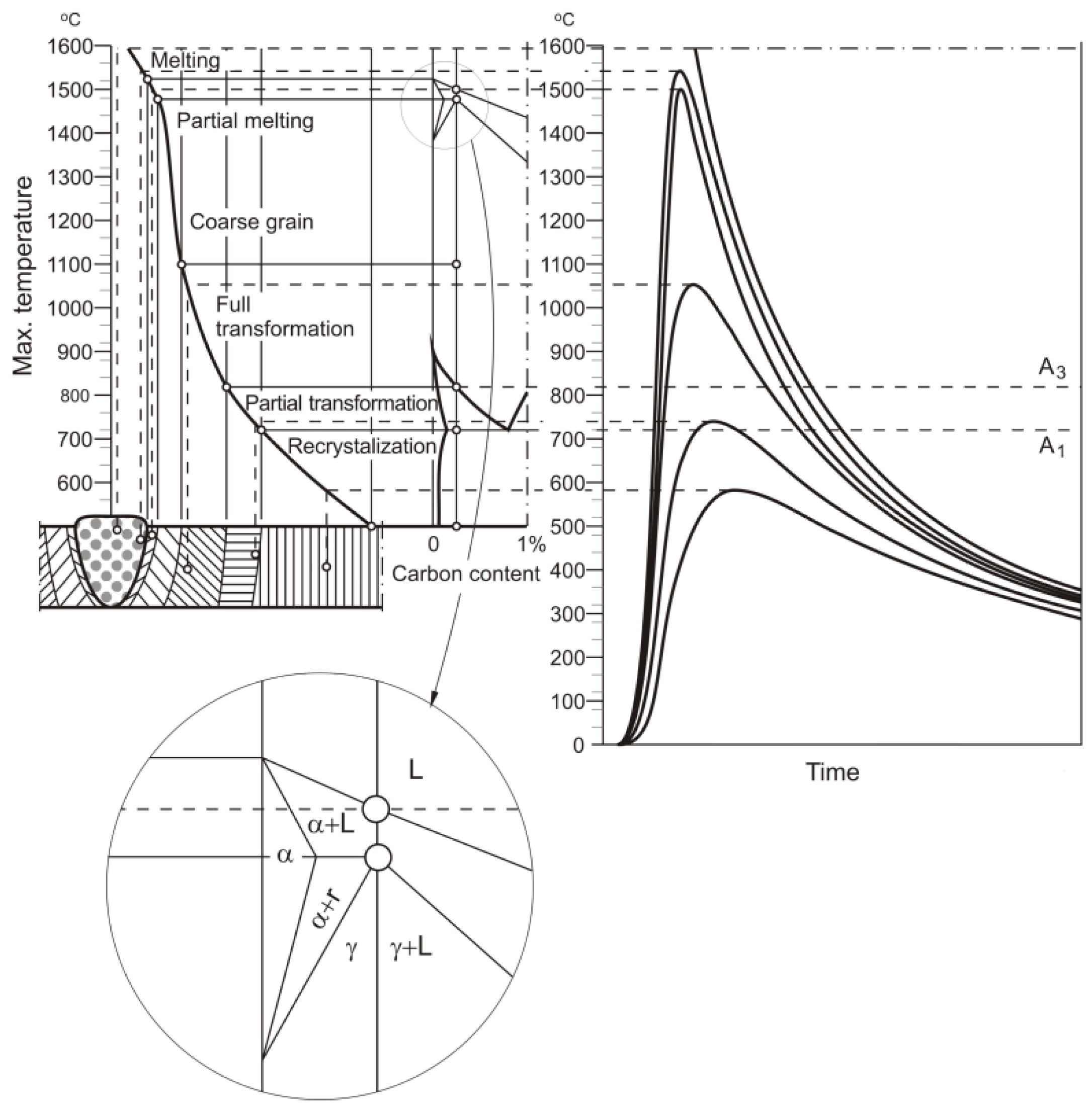
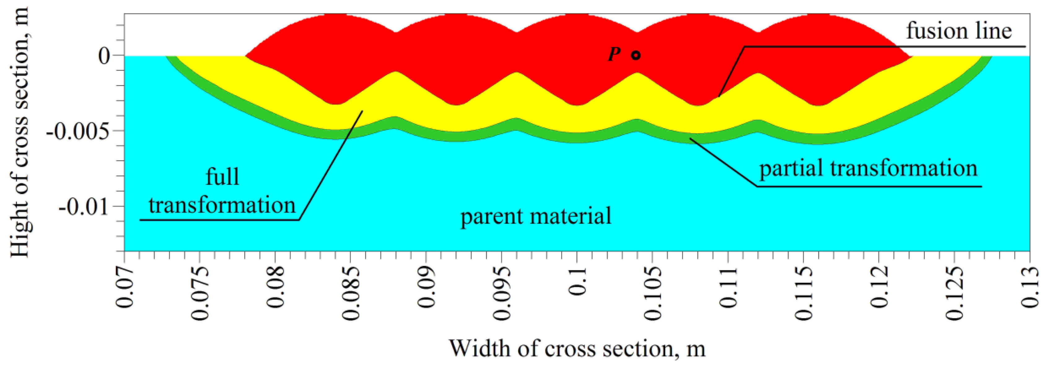
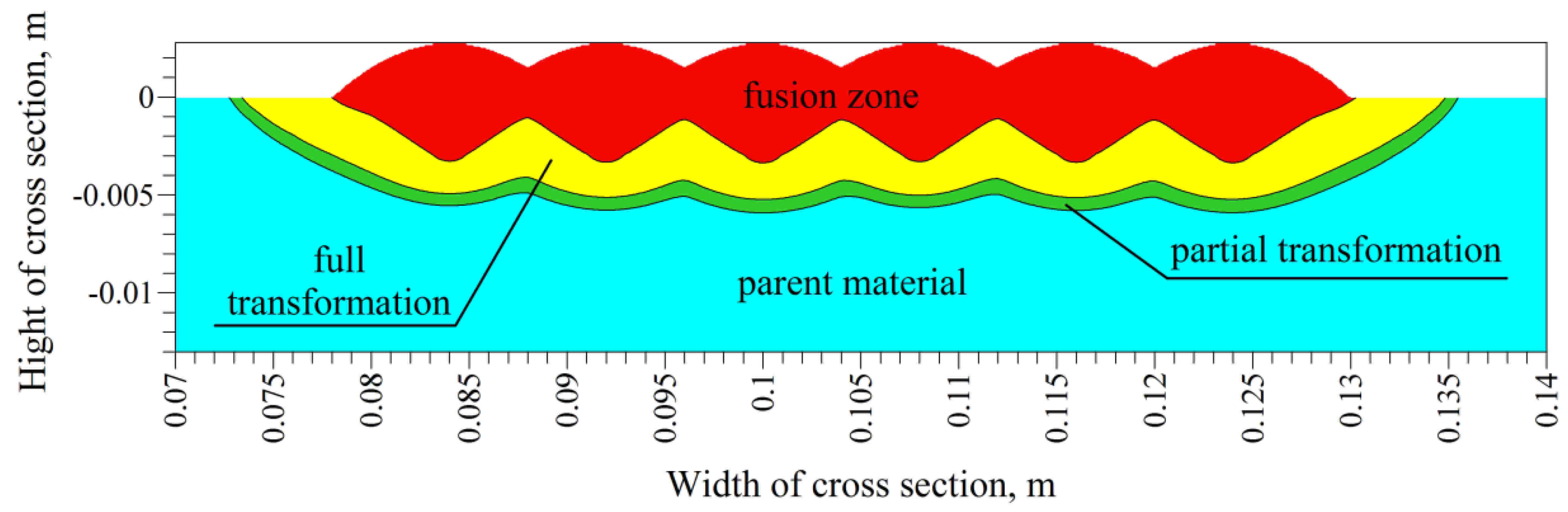
The temperatures reached during heating, the hold time at each temperature, including the cooling rate in the temperature range of 800–500 °C, determine the nature of structures that occur in junction during and after welding. The above-mentioned transformations caused by a welding thermal cycle result in shaping distinctive structural zones of the surfaced area (Figure 1):

-

fusion zone which is completely melted and has a dendritic solidification structure,

-

full transformation, when there is a complete transformation of the primary structure in austenite,

-

partial transformation,

-

the parent material, when there have been no phase transformations.

During heating, austenite transformation takes place whose beginning and end are limited by temperatures A₁ and A₃ resulting from the phase equilibrium Fe–C diagram. If the maximum heating temperature exceeds the temperature of the beginning of the austenite transformation A₁, but does not exceed A₃, there is incomplete austenitic transformation, i.e. only part of the original structure (parent material) is transformed into austenite. However, if the temperature exceeds A₃, then primary structure is completely transformed into austenite. Solidus temperature (above which the material begins to melt) defines the fusion line, and the area heated above this temperature creates a fusion zone.

In modeling of a temperature field in welding processes in the vast majority of solutions, the assumed heat source model is characterized by a direct effect of the entire amount of generated electric arc heat on the welded or surfaced object.

When welding, the weld execution takes place within the operation area of the welding arc and, by chamfering the edges of connected elements an area filled with liquid metal is determined. The fusion line is often of regular shape (usually parabolic) as well as isotherms in a heat-affected zone. However, during surfacing by welding of flat surfaces the fusion line shape is often irregular. Single-distributed heat source models accepted in the description of temperature fields do not allow one to reconstruct irregular isotherm shapes (including the fusion line). Therefore, a bimodal model is proposed.

3. The Analytical Description of the Temperature Field during Multi-Pass Surfacing

The bimodal model of the heat source in description of the temperature field during surfacing by welding is applied, finding justification in the way of transmitting heat generated by an electric arc to the surfaced object. In this model, only one heat source is physically present—an electric arc. It is assumed that part of the heat generated by the electric arc is transferred to the surfaced object by the direct impact of an electric arc. In contrast, part of the heat generated by the electric arc is consumed to heat up the electrode’s material, its melting and further heating up, until the melted material of an electrode in the form of droplets is detached under the influence of electromagnetic forces and transferred to the developing weld under their own weight.

In the analytical solutions, the influence of phase transformation heat (both solid and liquid) is generally ignored, thermo-physical properties of the material are assumed to be independent of temperature, and only the conduction effect is taken into consideration (the radiation phenomenon and the gravity field are omitted), also Joule heat (for electric arc welding) is omitted [6,7,8,9,10,11,12,13,14,53,54,55,56,57,58]. Such assumptions were also adopted in this work.

The point of departure in the description of the temperature field in a homogeneous and isotropic body is a basic differential equation of heat conduction based on the law of conservation of energy [53]. On the basis of the solution to this equation for a semi-infinite body with a moving heat source presented by Radaj [54] and Easterling [55], the author of this article describes the temperature field caused by an electric arc during single-pass surfacing, assuming a volumetric model of the heat source [59].

In the paper, it is assumed that the volume of electrode’s melted material is equal to the volume of the weld reinforcement and the amount of heat stored in the melted electrode’s material equals the quantity of heat transferred to the weld. Furthermore, it is assumed that the wire speed determines the speed of its melting. Taking into account the direct impact of an electric arc, as well as the heat transferred by the applied metal, the author determines analytically the temperature field during single-pass surfacing [60]:

$$T\left(x,y,z,t\right)-T_0=T_w\left(x,y,z,t\right)+T_a\left(x,y,z,t\right),$$

(1)

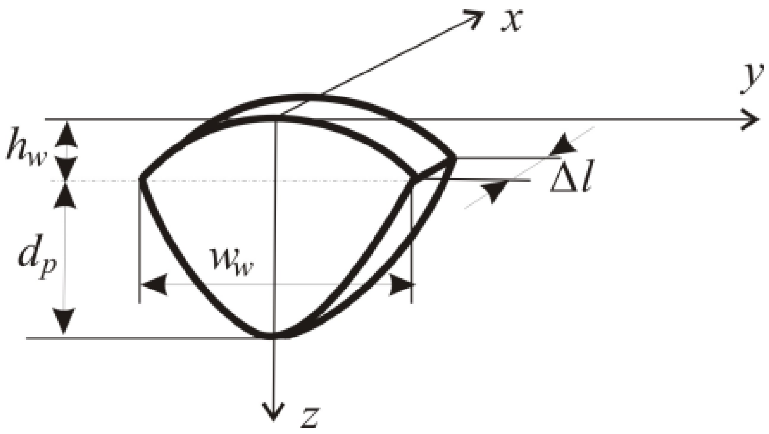
where T_w(x, y, z, t) and T_a(x, y, z, t) are temperature fields caused by heat of the weld reinforcement (used to melt the electrode) and direct influence of an electric arc respectively, while T₀ denotes initial temperature. For the weld a volumetric model of the heat source is assumed, the lower limit of which is the shape of welded surface, which in turn is assumed in the solution as flat or parabolic (Figure 2). The face of the weld is determined mainly by surface tension forces. Based on experimental research, Hrabe et al. [61] proposed the parabolic shape of the face of the weld. Therefore, in this work the face of the weld is assumed to be parabolic.

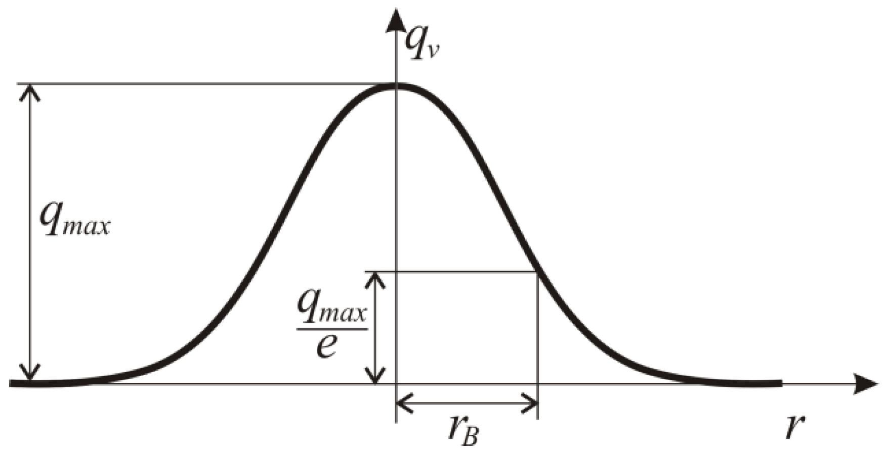
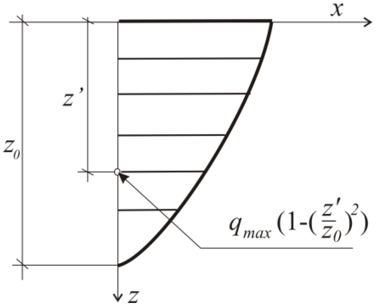
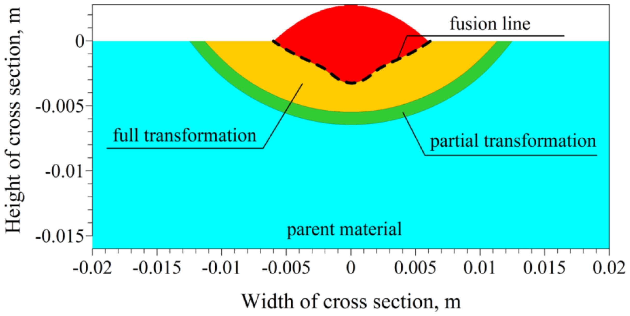
For the description of the temperature field caused by an electric arc a volumetric heat source of Gaussian surface distribution is assumed (Figure 3) and parabolic change in relation to depth (Figure 4) [59]. Calculations of the temperature field are performed for a single-pass surfaced S235 steel plate. The accuracy of solution is verified comparing the calculated fusion line to that obtained experimentally by other authors [61]. In the calculations, the same technological parameters as in the experiment were assumed. In Figure 5, the calculated heat-affected zone and fusion line obtained experimentally [62] are presented. The calculated fusion line coincides with the line obtained in experiment.

In the temperature field modeling during multi-pass surfacing, it is necessary to take into account temperature increments, caused by overlaying consecutive welding sequences and self-cooling of areas previously heated.

Since during surfacing weld overlaps (30% to 60% of the cross-sectional area of the deposit) are used in order to obtain a smooth weld surface, in the numerical model the distances between the axes of the welds must be adequately smaller than the width of the weld.

For the proper mapping process, auxiliary time connected with the idle movement of an electrode (welding head) or other activity resulting from the needs of technological processing (e.g., correction or change of technological parameters) should also be considered.

Then, the temperature field during the application of k-th weld is determined by:

$$T\left(x,y,z,t\right)-T_0={\displaystyle \sum _{j=1}^{k-1}\Delta T_j^C}+\Delta T_k^H,$$

(2)

where Δ$T_j^C$ denotes the increment of temperature caused by the already applied (cooling) j-th weld, while Δ$T_j^H$ the increment of temperature during application of k-th weld. Whereas the temperature field after application of all welds is described by:

$$T\left(x,y,z,t\right)-T_0={\displaystyle \sum _{j=1}^k\Delta T_j^C}.$$

(3)

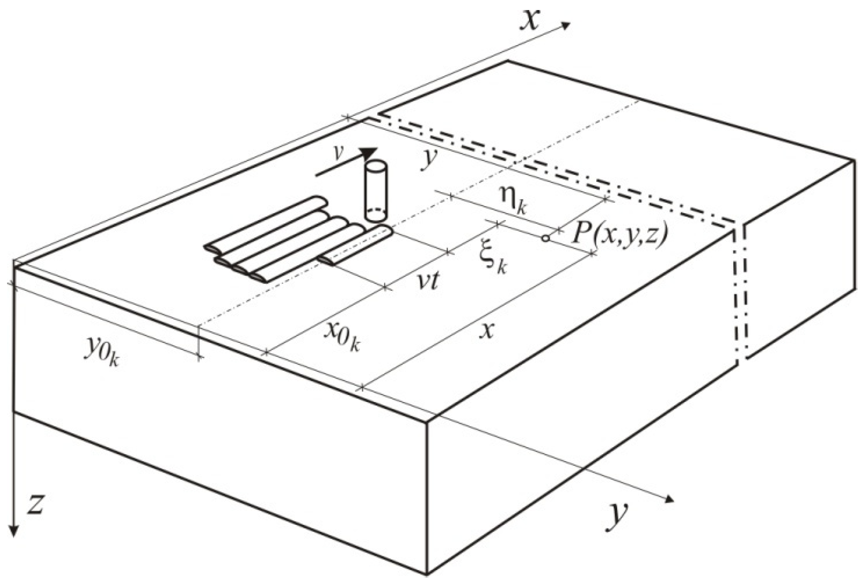
On the basis of solution for single-pass surfacing [60] the temperature increment at point P(x, y, z) during multi-pass surfacing (Figure 6) can be described by the following equations:

For time t ≤ t_c, where t_c means the total time of welds application:

$$\begin{array}{l}T\left(x,y,z,t\right)-T_0=\hfill \\ ={\displaystyle \sum _{j=1}^{k-1}\{A_w{\displaystyle \underset{t_{bj}}{\overset{t_{ej}}{\int }}\{H_C\left(t\prime \right)}\left(G_2(y,z)+G_3(y,z)-G_4(y,z)-G_1(y,z)\right)\}dt\prime }+A_C{\displaystyle \underset{t_{bj}}{\overset{t_{ej}}{\int }}{F}_C(t\prime )dt\prime }\}+\hfill \\ +A_w{\displaystyle \underset{t_{bk}}{\overset{t}{\int }}\{H_H(t\prime \prime )}\left(F_2(y,z)+F_3(y,z)-F_4(y,z)-F_1(y,z)\right)\}dt\prime \prime +A_k{\displaystyle \underset{t_{bk}}{\overset{t}{\int }}{F}_H(t\prime \prime )dt\prime \prime }\hfill \end{array},$$

(4)

for time t > t_c:

$$\begin{array}{l}T\left(x,y,z,t\right)-T_0=\\ ={\displaystyle \sum _{j=1}^k\{A_w{\displaystyle \underset{t_{bj}}{\overset{t_{ej}}{\int }}\{H_C\left(t\prime \right)}\left(G_2(y,z)+G_3(y,z)-G_4(y,z)-G_1(y,z)\right)\}dt\prime }+A_C{\displaystyle \underset{t_{bj}}{\overset{t_{ej}}{\int }}{F}_C(t\prime )dt\prime }\}\end{array},$$

(5)

where

$$A_w=\frac{{\dot{q}}_v}{8C_p\mathsf{\rho }\sqrt{\mathsf{\pi }a}},$$

(6)

$$H_H(t\prime \prime )=\frac{1}{\sqrt{t\prime \prime }}\left(\mathrm{erf}\left(\frac{\Delta l-2\left(\mathsf{\xi }+vt\prime \prime \right)}{4\sqrt{at\prime \prime }}\right)+\mathrm{erf}\left(\frac{\Delta l+2\left(\mathsf{\xi }+vt\prime \prime \right)}{4\sqrt{at\prime \prime }}\right)\right),$$

(7)

$$H_C\left(t\prime \right)=\frac{1}{\sqrt{\left(t-t\prime \right)}}\left(\mathrm{erf}\left(\frac{\Delta l-2\left(x-vt\prime -x_0\right)}{4\sqrt{a\left(t-t\prime \right)}}\right)+\mathrm{erf}\left(\frac{\Delta l+2\left(x-vt\prime -x_0\right)}{4\sqrt{a\left(t-t\prime \right)}}\right)\right),$$

(8)

$$A_k=\frac{3\dot{q}}{8C_p\mathsf{\rho }\mathsf{\pi }a{z}_0}\exp \left(-\frac{v{\mathsf{\xi }}_k}{2a}-\frac{v^2{t}_0}{4a}\right),$$

(9)

$$\begin{array}{l}{F}_H(t\prime \prime )=\frac{1}{t\prime \prime +t_0}\exp \left(-\frac{{{\mathsf{\xi }}_k}^2+{{\mathsf{\eta }}_k}^2}{4a\left(t\prime \prime +t_0\right)}-\frac{v^{2}t\prime \prime }{4a}\right)\\ \{\left(1-\frac{z^2+2at\prime \prime }{z_0^2}\right)\mathrm{erf}\left(\frac{z+z_0}{2{\left(at\prime \prime \right)}^{0,5}}-\mathrm{\Phi }\left(z\right)\mathrm{erf}\left(\mathrm{\Phi }\left(z\right)\frac{z-z_0}{2{\left(at\prime \prime \right)}^{0,5}}\right)\right)+\\ \frac{4at\prime \prime }{z_0^2}\left(\frac{z+z_0}{{\left(4\mathsf{\pi }at\prime \prime \right)}^{0,5}}\exp \left(-\frac{{\left(z-z_0\right)}^2}{4at\prime \prime }\right)-\frac{z-z_0}{{\left(4\mathsf{\pi }at\prime \prime \right)}^{0,5}}\exp \left(-\frac{{\left(z+z_0\right)}^2}{4at\prime \prime }\right)\right)\}\end{array},$$

(10)

$$A_C=\frac{3\dot{q}}{8C_p\mathsf{\rho }\mathsf{\pi }a{z}_0},$$

(11)

$$\begin{array}{l}{F}_C(t\prime )=\frac{1}{t+t_0-t\prime }\exp (-\frac{{\left(x-vt\prime -x_{0j}\right)}^2+{\left(y-y_{0j}\right)}^2}{4a\left(t+t_0-t\prime \right)})\\ \{\left(1-\frac{z^2+2a\left(t-t\prime \right)}{z_0^2}\right)(erf\left(\frac{z+z_0}{2{(a(t-t\prime ))}^{0,5}}\right)-\mathrm{\Phi }\left(z\right)erf\left(\mathrm{\Phi }\left(z\right)\frac{z-z_0}{2{(a\left(t-t\prime \right))}^{0,5}}\right))+,\\ \frac{4a\left(t-t\prime \right)}{z_0^2}\left(\frac{z+z_0}{{\left(4\mathsf{\pi }a\left(t-t\prime \right)\right)}^{0,5}}\exp \left(-\frac{{\left(z-z_0\right)}^2}{4a\left(t-t\prime \right)}\right)-\frac{z-z_0}{{\left(4\mathsf{\pi }a\left(t-t\prime \right)\right)}^{0,5}}\exp \left(-\frac{{\left(z+z_0\right)}^2}{4a\left(t-t\prime \right)}\right)\right)\}\end{array}$$

(12)

$${\mathsf{\xi }}_k=x-v\left(t-\left(k-1\right)\left(\frac{l_k}{v}+t_{pk}\right)\right)-x_{0k},$$

(13)

$$\mathrm{\Phi }(z)=\{\begin{array}{l}-1forz\in <0,z_{0i}>\\ 1forz\in (z_{0i},\infty )\end{array},$$

(14)

$$\dot{q}=\mathsf{\eta }UI-{\dot{q}}_v,$$

(15)

$$t_c=\frac{{\displaystyle \sum _j{l}_j}}{v},$$

(16)

where functions F₁(y, z)–F₄(y, z) and G₁(y, z)–G₄(y, z) are solutions of integrals using Gauss-Legendre quadrature described in the appendix, a denotes thermal diffusivity (m²/s), C_p—specific heat (J/kg K), ρ—density (kg/m³), z₀ (m) denotes the depth of heat source deposition, and quantity t₀ (s) characterizes the surface heat source distribution thus satisfying the relation (cf. Figure 3):

$$r_B^2=4a{t}_0,$$

(17)

where the r_B denotes the averaged radius of heat source with Gaussian distribution [63], U (V), I (A) and η voltage, current and arc efficiency respectively, v (m/s)—velocity of heat source (welding speed), t_bj (s) and t_ej (s)—denote starting and finishing time of applying j-th weld, defined as:

$$t_{bj}=\left(j-1\right)\left(\frac{l_j}{v}+t_{pj}\right),$$

(18)

$$t_{ej}=\left(j-1\right)t_{pj}+j\frac{l_j}{v},$$

(19)

l_j (m)—the length of j-th weld with coordinates x_0j and x_kj:

$$l_j=x_{kj}-x_{0j},$$

(20)

t_pj auxiliary time preceding the application of j-th weld.

The total amount of heat q_v contained in the material of a melted electrode is expressed by the relationship [64]:

$$q_v=\Delta q_{solid}+\Delta q_f+\Delta q_{liqiud},$$

(21)

where Δq_solid—heat necessary to heat up the electrode from the initial temperature to the melting temperature, Δq_f—heat used for melting the electrode (heat of fusion), Δq_liquid—heat used for heating up melted material to the temperature T_L, in which the drop of metal falls on the surface of the welded material.

The value of the initial temperature of the electrode T_e from the welding head is set at 100 °C. In correspondence to the above:

$${\dot{q}}_v=\dot{m}\left(C_p\left(T_L-T_e\right)+L\right),$$

(22)

where

$$\dot{m}={\mathsf{\rho }}_e\frac{\mathsf{\pi }{d}^2}{4}{v}_e,$$

(23)

v_e (m/s)—velocity of passing electrode wire with diameter d (m) and density ρ_e (kg/m³).

4. Example of Calculations

Calculations of the transient temperature field are conducted for a steel element with a length of 500 mm, width of 200 mm, and thickness of 30 mm, made with commonly used weldable construction steel S235.

Numerical simulations were performed with the author's program created in Borland Delphi environment using Borland Pascal language. In the program, the integration procedure over time is implemented according to the trapezoidal method. Near the control area (cross-section—x = 0.25 m) calculations were performed at 0.01 s with division of the integration interval at 0.0002 s. Calculations with such a time increase and with the division of the integration interval are necessary due to the high heating rates, as well as reaching maximum temperature at particular points of surfaced object at different times of the deposition process. In the anticipated areas and the heat-affected zone, temperature calculations were made at points in the distances of 1 mm, increasing the distance further from the HAZ—at the edges of the plate calculation were performed every 1 cm.

Thermal properties of the welded material and electrode are determined by a = 8 × 10⁻⁶ m²/s, C_p = 670 J/kg K, ρ = 7800 kg/m³ and L = 268 kJ/kg.

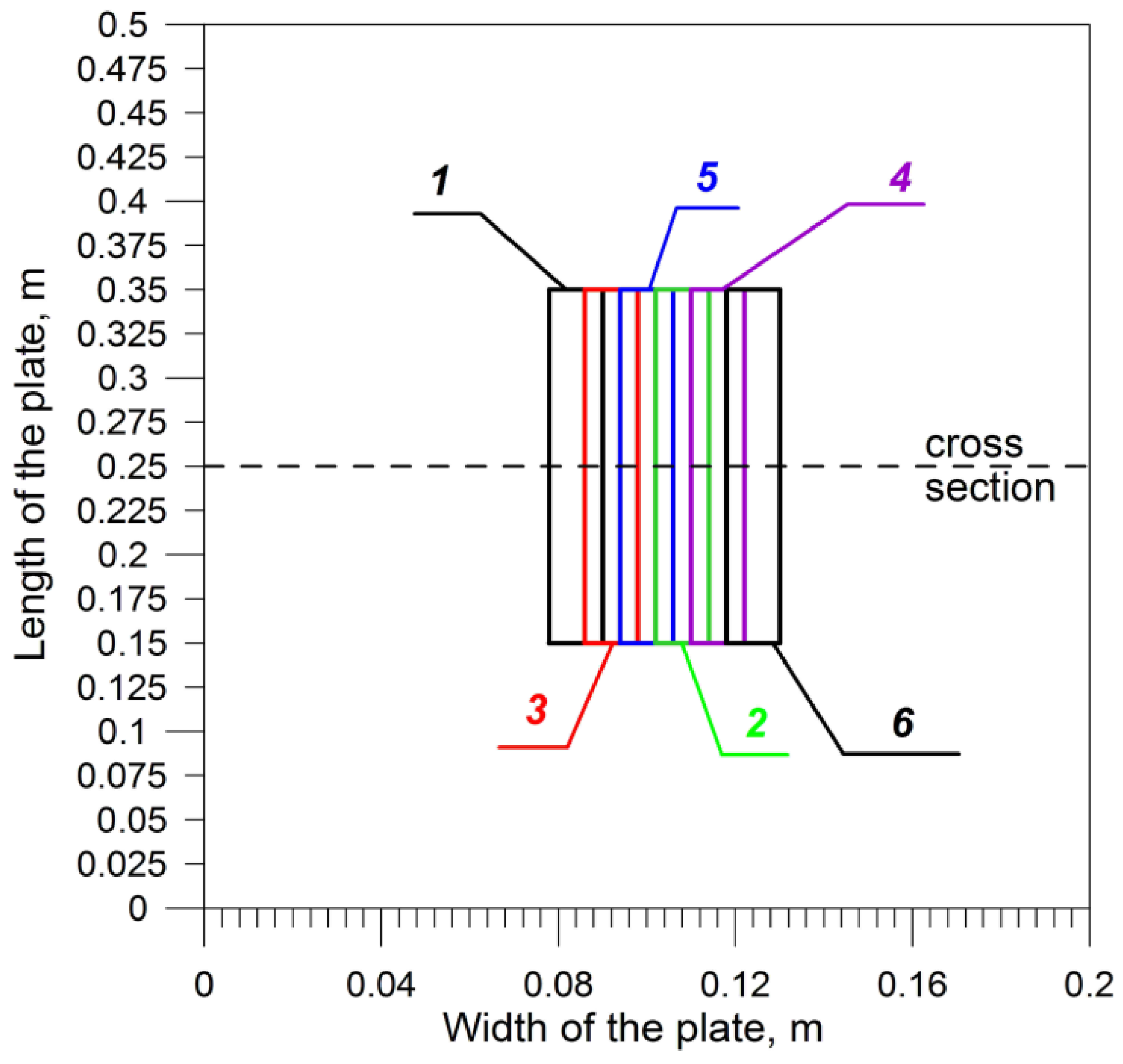
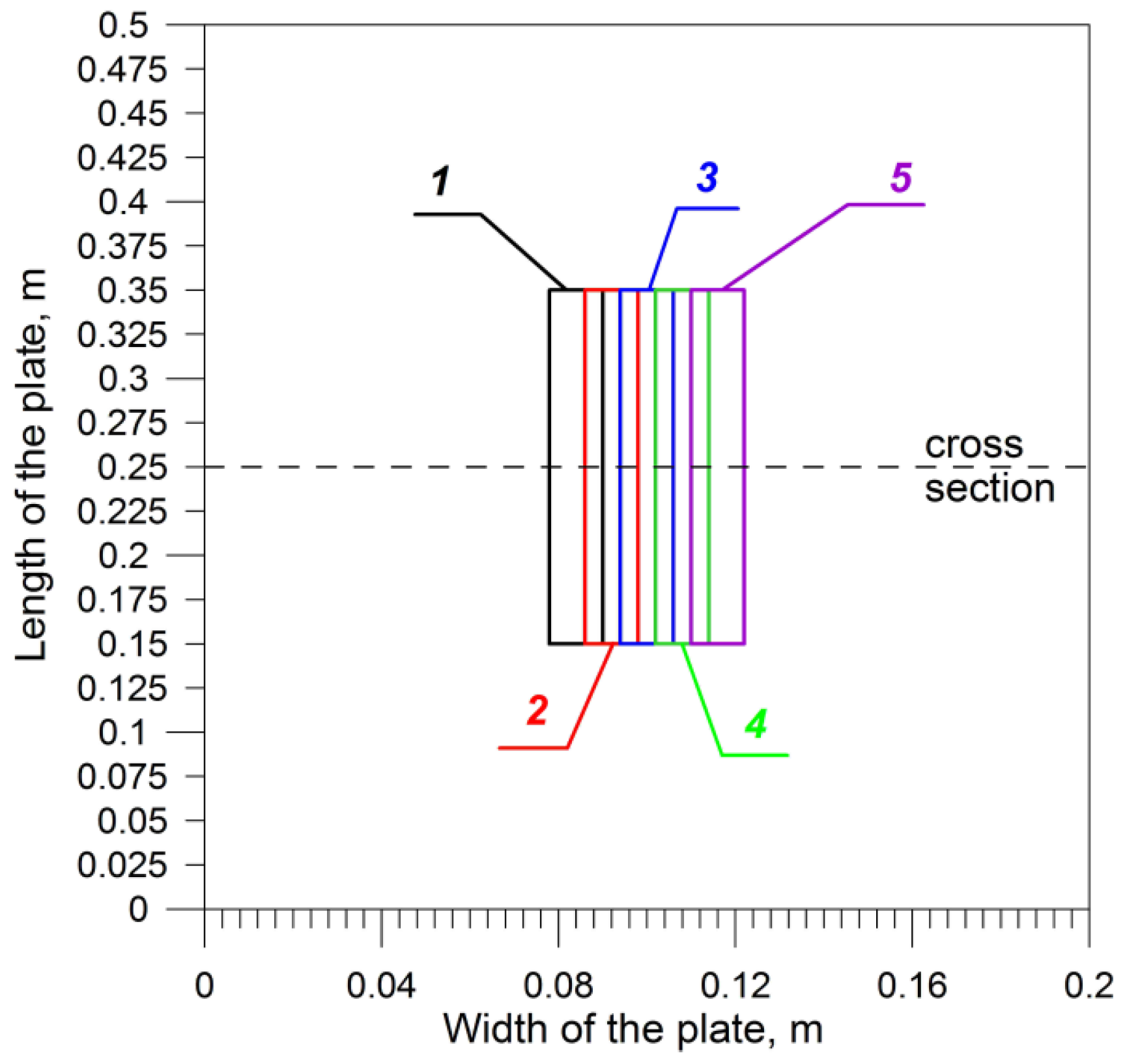
In the simulation, five welds are applied in the middle part of a welded element (the coordinate of weld beginning x₀ = 0.15 m) of length l = 0.2 m. The surfaced area on the top surface of the plate with sequence of the weld padding is presented in Figure 7, where a dashed line denotes the location of a cross-section, at which the analysis of the temperature distribution and welding thermal cycles was performed.

The numerical simulation is conducted for the welding heat source of power 3500 W, which corresponds to the parameters U = 24.3 V, I = 232 A, η = 0.6 applied in trials of single-pass GMA surfacing conducted by Klimpel et al. [62]. The source connected with the activity of an electric arc with Gaussian distributed power density is characterized by z₀ = 0.0062 m and t₀ = 0.001 s. Likewise, in calculations for an experiment, welding speed v = 0.007 m/s, electrode wire diameter d = 1.2 mm, wire feed speed v_e = 0.013 m/s and bead dimensions h_w = 2.77 mm, w_w = 11.93 mm (d_p = 0) are assumed. In the calculations, the assumed chemical composition and properties of the electrode material (wire SG3 DIN 8559) are similar to the material of the overlaid object. Accordingly, the content of the article has been completed. Additionally, there are initial values of the temperature of electrode T_e = 100 °C and temperature T_L = 2500 °C assumed. The weld overlap is obtained assuming the distance between axes of particular beads equal to 8 mm.

The transient temperature distribution in the area surrounding the weld of a cross-section, halfway down the welded element is presented in Figure 8, Figure 9, Figure 10 and Figure 11: during the application of the second weld at time 0.2 s and 0.4 s after the passage of an electrode (Figure 8 and Figure 9) and during the application of the fourth weld at time 0.3 s and 0.5 s after the passage of an electrode (Figure 10 and Figure 11).

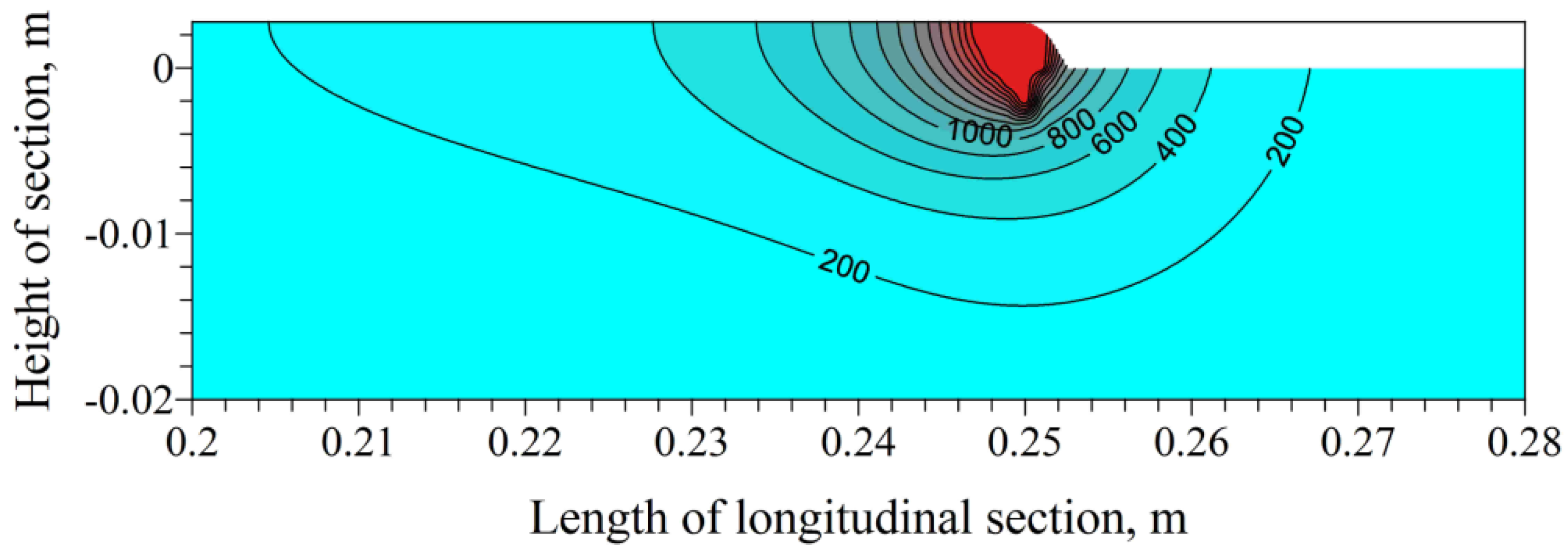
In Figure 8 and Figure 10, one can observe a strong influence of the weld reinforcement heat on temperature isotherm in neighboring, previously created padding welds. The temporal temperature field during the application of the third weld at time t = 83 s (electrode’s position x = y = 0.1 m) is presented in Figure 12 (in longitudinal section on the axis of third weld) and in Figure 13 (on the top surface of a surfaced element z = 0). The obtained shapes of the heat-affected zone determined by isotherms are confirmed in the literature, for example [31,41].

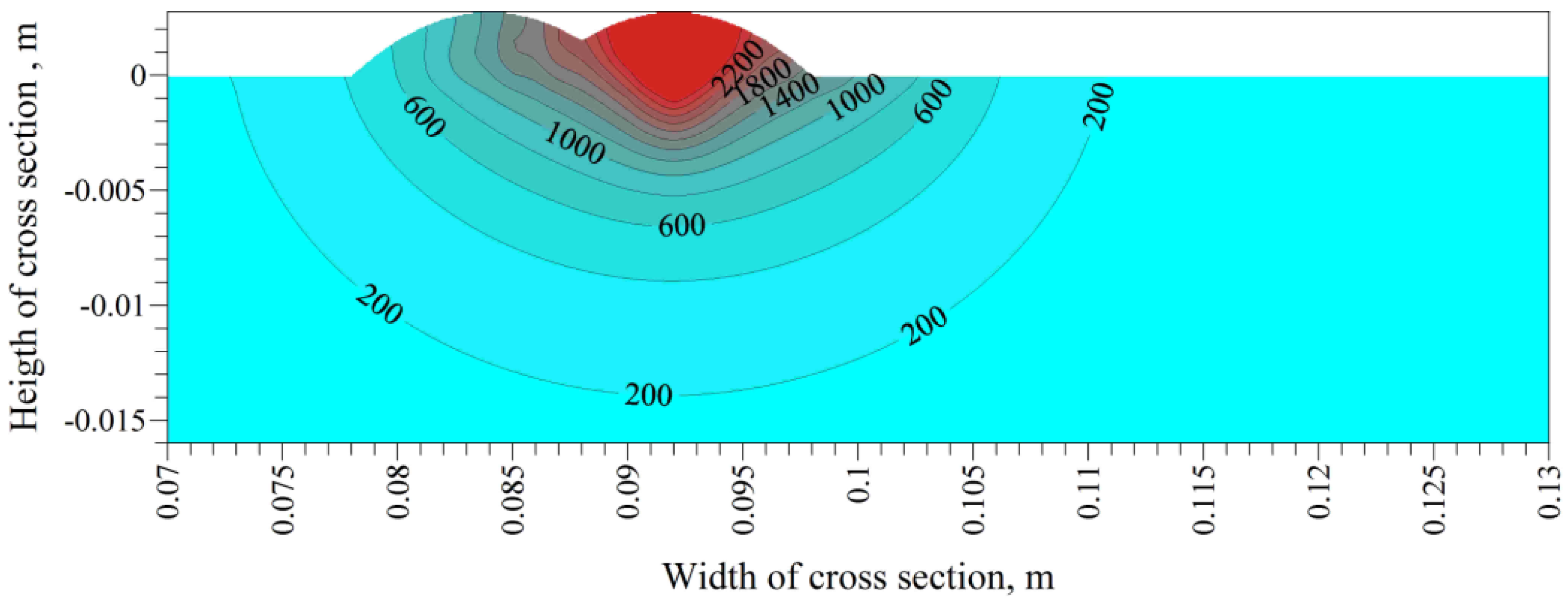
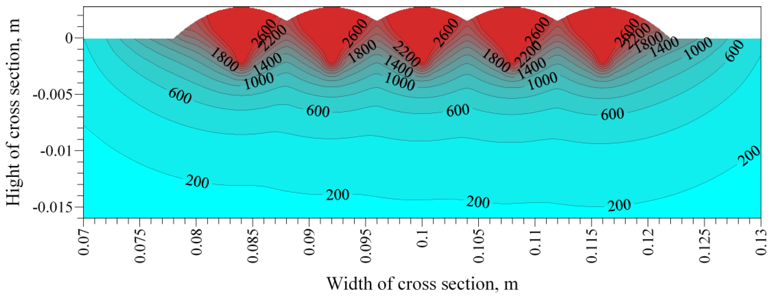
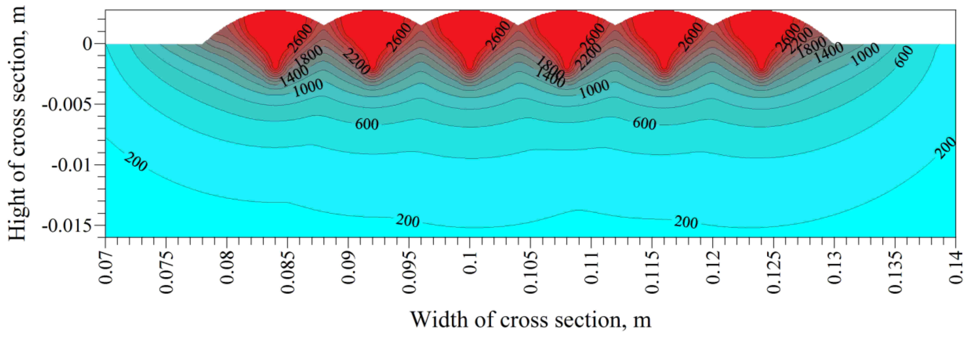
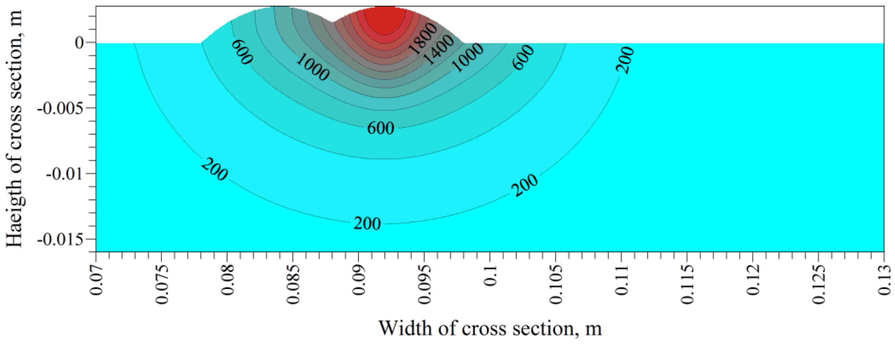
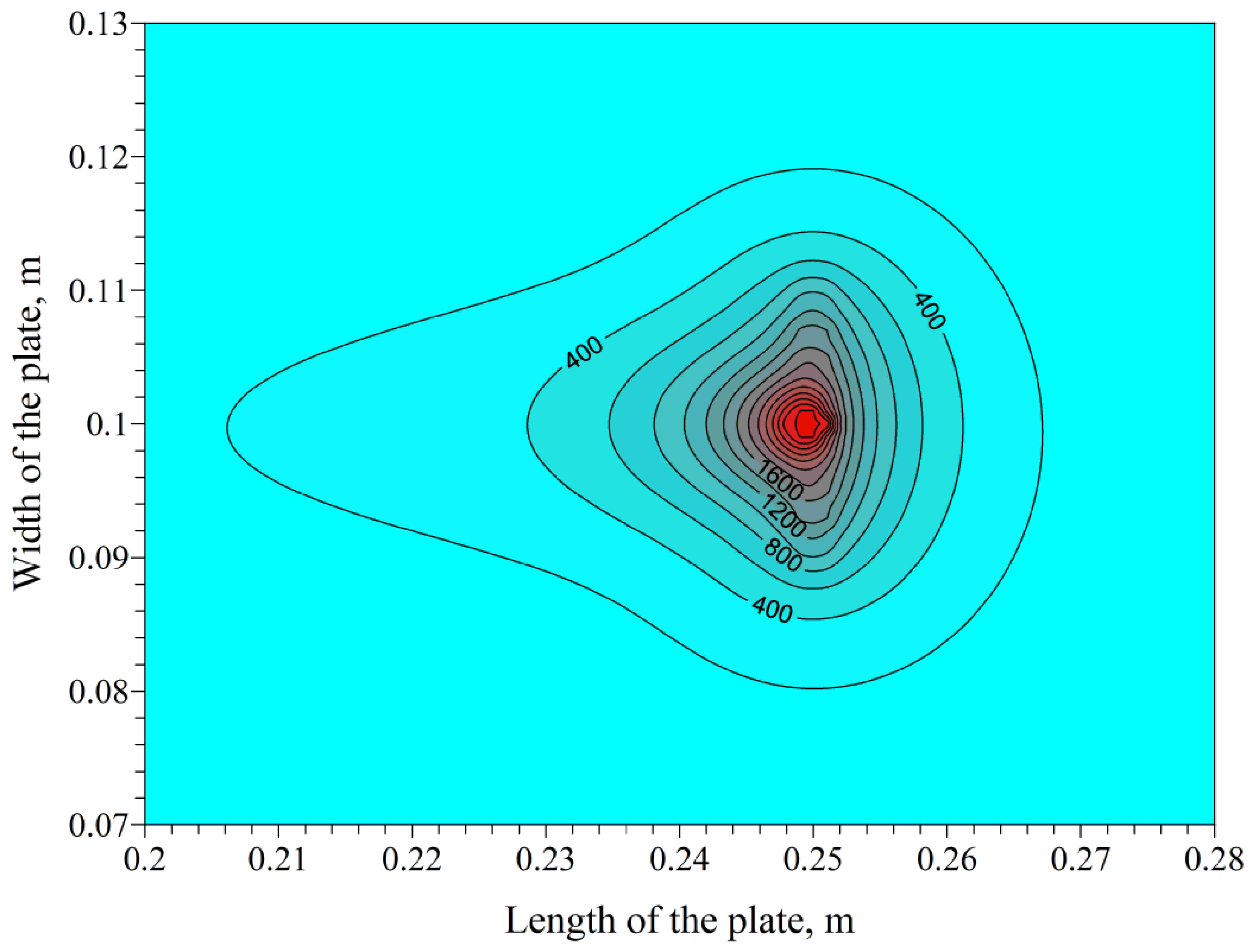
Isotherms of maximum temperature obtained during the whole surfacing process in the cross-section of the element (the peak temperature contour experienced for all welds) and in the heat-affected zone are illustrated in Figure 14 and Figure 15. The field of maximum temperature shows clear asymmetry outside the heat-affected zone.

The depth of deposition of the heat-affected zone is determined by the initial and final temperatures of austenitization A₁ = 723 °C and A₃ = 835 °C, while a fusion line by the solidus temperature 1493 °C is presented in Figure 16. The depth is increasing with subsequent welds—after five beads, an increase of 0.5 mm is observed. Larger depth of fusion is the result of short padding welds, which have not cooled to the initial temperature before applying the next bead, which in turn resulted in the accumulation of heat in the surfaced area, and temperature increase. In Figure 16, point P is marked with coordinates (0; 0.104), for which thermal cycles are presented in Figure 17. At this point, the phase transformations occur twice, including melting of the material.

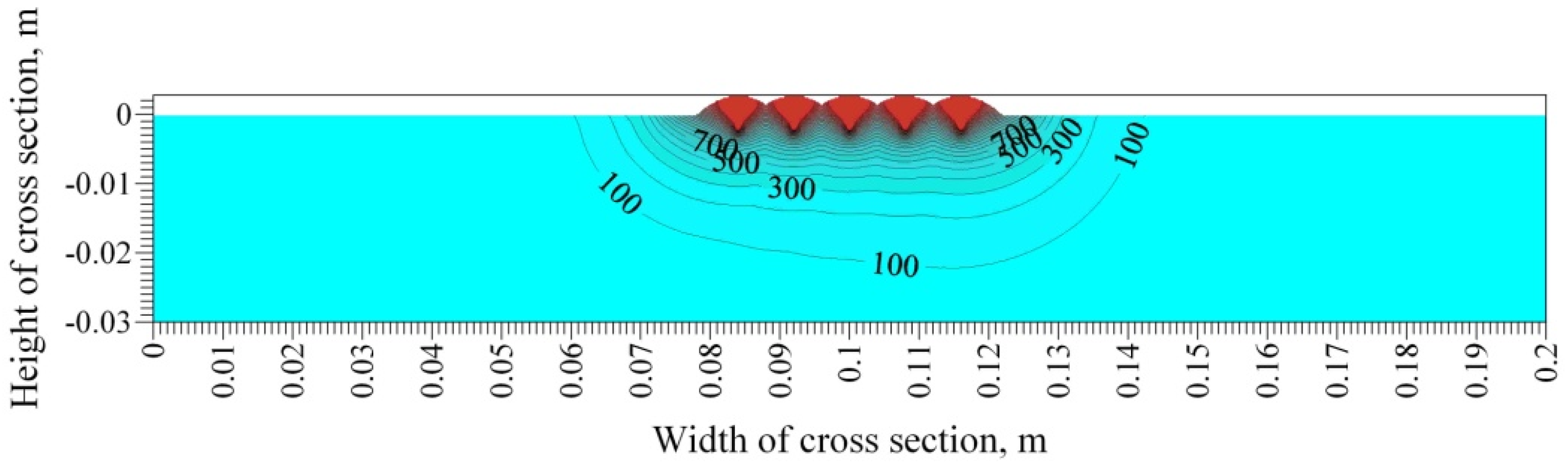
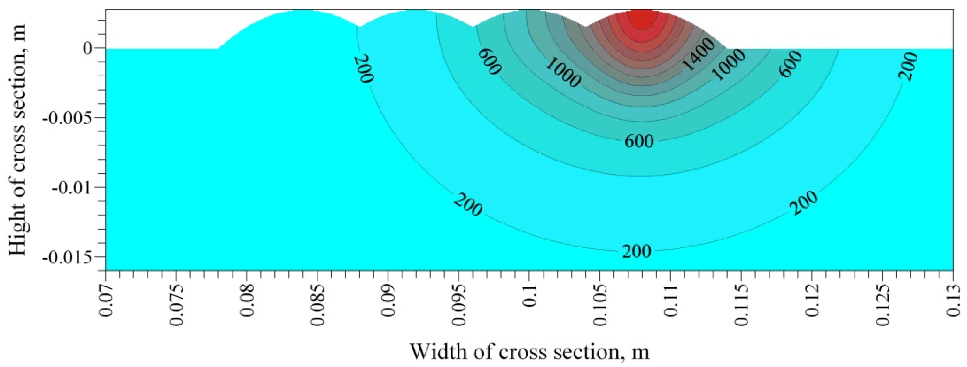
In order to determine the influence of sequence of imposed padding welds on the shape and dimensions of the heat-affected zone, the temperature field was calculated with the same technological parameters of the deposition process, but simulating alternate welds padding (Figure 18).

The alternate execution of individual beads allowed one to obtain an even distribution of the maximum temperature reached in the cross-section of the surfaced object throughout the surfacing process (Figure 19) as well as the same dimensions of the heat-affected zones for the individual beads (Figure 20).

The disadvantage is the computation time for a full heat analysis (for the analyzed example in the article, computation time on a 4-core 2.3 GHz processor computer amounted to a few days). The computation time can be reduced by increasing the pace of integration over time, although this also reduces the accuracy of the calculations.

5. Conclusions

As part of the heat generated by an electric arc is used to melt the electrode material, which in the form of droplets falls into the weld pool, it is necessary to take into consideration the heat of the molten metal in the temperature field descriptions in arc weld surfacing processes. In this work, the analytical solution of the temperature field of multi-pass arc weld surfacing for a semi-infinite model of body is presented. The solution is obtained by adding together the temperature increments caused by the application of liquid metal and thermal radiation from the electrode as well as from the areas already heated up. The analytical model also considered a weld overlap and auxiliary time connected with the idle movement of electrode (welding head) or other activity resulting from the needs of technological processing (e.g., correction or change of technological parameters).

For the applied metal, the heat source of parabolic shape in the cross-section of a weld is assumed. For the electric arc, the source with Gaussian surface distribution of power density is assumed. The dimensions of the weld and technological parameters of the process were adopted from the experience of other authors. The amount of heat transmitted by the applied padding weld was determined on the basis of the heat cumulated in the electrode melted material. Calculations of the temperature field during multi-pass arc weld surfacing are conducted on a steel plate.

Analysis of the temperature fields in the control cross-section showed a slight increase in the depth of the heat-affected zone when performing successive beads. This is due to the relatively short times between successive passages of the heat source in a sectional view. Also noticeable is the influence of heat of applied padding welds on those previously imposed causing an increase in temperature in the areas of reinforcements (reinforcements). This effect can be reduced by (often used in practice) alternate padding welds application, increasing the time between the passages of the weld heat source over particular areas of the surfaced element.

The presented model has a significant meaning especially in temperature field computations during the application of high (a few millimeters) and wide (a dozen or so millimeters) welds, because the expected dimensions of the welds are also the geometrical parameters of the volumetric model of the weld heat source.

The adoption of a bimodal heat source allowed the reconstruction of the irregular shape of the fusion line, often found in welding practice and impossible to obtain using a single-distributed heat source. In the description of the temperature field, the heat of the molten electrode has been taken into account. This approach brings the model closer to the real phenomena occurring in the welding process. The description of the temperature field is obtained by the analytical solution for multi-pass weld surfacing, unprecedented in the literature with the use of something other than a point heat source. The adopted algorithm allows one to analyze the influence of the surfacing sequence on the shape and dimensions of the heat-affected zone.

The advantage of an analytical model of the temperature field is the possibility of quick analysis of welding thermal cycle at any point of the surfaced object without determining temperatures in the whole object, as well as the possibility to easily track temperature changes for selected cross-sections of an object in the selected time of the process.