Dynamic Similitude Design Method of the Distorted Model on Variable Thickness Cantilever Plates

Abstract

In the present study, a new method of predicting the dynamic behavior of a variable thickness (VT) cantilever plate by using a thin plate scaled model is proposed. The thin plate model, defined as the model thin (MT) plate, is designed by using the newly proposed similitude design method. The method is derived based on the transfer matrix of both the stepped thickness (ST) plate that is simplified by the VT plate and the thin plate. The thickness of the MT plate is calculated by introducing the equivalent thickness corresponding to each VT plate’s vibration modals, such that a series of accurate distorted scaling laws are provided to predict each corresponding property. Moreover, an algorithm of designing the MT plate is proposed and a design process is summarized in steps. Finally, an example, where the prototype VT plate is made of 42 CrMo and the MT plate is made of NO. 45 steel, is discussed to validate the proposed design method, showing that the MT plate, which is designed by using the proposed method, can accurately predict the dynamic properties of the prototype VT plate, and showing its significance in engineering practice.

1. Introduction

Variable thickness (VT) plates have been widely applied in engineering practice such as, for example, advanced gas turbines, high-powered aircraft jet engines and high-speed centrifugal separators [1,2,3]. The vibration problems of the plate structures in these engineering machines are important for consideration in the design process [4,5,6].

By using the finite element method, vibration problems of VT plates are widely studied. Huang et al. [7] investigated the free vibration problem of orthotropic rectangular VT plates by using a discrete method. Based on the Green function, Sakiyama et al. [8] discussed an approximate method for analyzing the free vibration of rectangular VT plates, and Guo et al. [9] introduced a dynamic function in the finite strip method, where numerical analysis was used to demonstrate the application of the approaches by analyzing simply supported stepped thickness (ST) plates. It has been shown that the numerical solutions of the approximate method had good accuracy for various types of rectangular plates with uniform or non-uniform thickness.

Moreover, Eisenberger and Jabareen [10], in 2001, computed exact axisymmetric vibration frequencies of VT circular and annular plates by approximating the variation in thickness into an infinite power series. Jiang and Redekop [11] studied the free vibration characteristics of linear elastic orthotropic toroidal VT shells based on the Sanders–Budiansky shell equations, and Kang and Leissa [12] also discussed the free vibration on VT paraboloids shells by using a three-dimensional method. Recently, based on the polynomial fitted thickness, VT plates’ various combinations of boundary conditions were investigated by Shufrin and Eisenberger [13], where two shear deformation plate theories were applied to provide accurate results in solving natural frequencies. By using the Generalized Differential Quadrature (GDQ) method, most recently, Tornabene et al. [14] and Bacciocchi et al. [15] investigated the free vibration of doubly-curved shells, singly-curved shells and plates with continuous thickness variation, showing that the GDQ method provides an accurate, stable and reliable numerical tool in analyzing variable thickness thin walled structures.

However, although theoretical studies have been widely discussed, experimental tests of the actual structure are still necessary. The issue is that, in practice, experimental investigation on thin walled structures like VT plates are actually expensive and time-consuming. Consequently, a scaled down model, which is usually designed based on similitude theory, is employed to reflect the prototype behavior. In general, due to the lack of the availability of materials, or the unavailability of members’ specified dimensions, researchers often use thin plates for the analysis [16,17], but this may limit the application of the test results.

Dynamic similitude design of thin walled plate structures is important in engineering practice and has been discussed by many researchers. For example, De Rosa et al. [18] investigated the distorted scaling laws in predicting the dynamic response of rectangular flexural plates based on the analysis of the vibration energy. Ramu et al. [19] considered the scaled model made of different materials to predict the dynamic behavior of the prototype by using a scaling law, which has been established based on dimension analysis, for free vibration. Qian et al. [20] established the scaling laws of laminated plates based on the governing equation analysis to predict the impulse response of the prototype. The results indicate that scaling laws can accurately predict the undamaged response of impact. Moreover, scaling laws of isotropic laminated plates have been studied by Ungbhakorn et al. [21]. In their study, governing equations of buckling and frequency were used to derive the scaling laws, and partial similitude was also considered, recommending the scaling laws with good accuracy. Rezaeepazhand et al. [22] studied the scaling laws of distortion models for predicting the laminate plate’s buckling and free vibration, deriving the scaling laws on different material and geometrical properties by using the governing equations of laminated plates and shells.

Basically, dynamical similitude design of complex structures, especially the design of distorted models, still focus on the distortion of materials. However, due to the structure’s complexity of the prototype, the study of geometrically distorted models is a real need. Most recently, Luo and Zhu et al. [23,24,25] presented a series of methods in the design of geometrically distorted models of plates and shells. In their work, the sensitivity analysis was employed in deriving accurate distorted scaling laws to predict the dynamic characteristics of the prototype [26,27]. In this study, in order to address the problem in designing a scaled model for a VT plate, a simplified ST plate, which has the same dynamic properties of the VT plate, is introduced. By using the transfer matrix method, the equivalent thickness of the corresponding thin plate is derived for each vibration modals. Then, a unified thickness of the Model Thin (MT) plate is selected and the corresponding scaling law is proposed such that the dynamic properties of the prototype VT plate can be predicted by using the MT plate.

The manuscript is organized as follows. In Section 2, the distorted scaling law of thin walled plates is derived based on the governing equation. The simplified ST plate is then proposed in Section 3, where the transfer matrices of both ST plates and thin plates with the cantilever boundary condition are discussed, and the equivalent thicknesses of different vibration modals are computed. In Section 4, the scaled down model of the VT plate is designed with a unified thickness, and the corresponding scaling laws are derived to predict the dynamic properties of the prototype VT plate. A case study is also provided to validate the proposed design method and a general process of designing the MT plate is summarized. Finally, conclusions are presented in Section 5.

2. Distorted Scaling Law of Thin Cantilever Plates

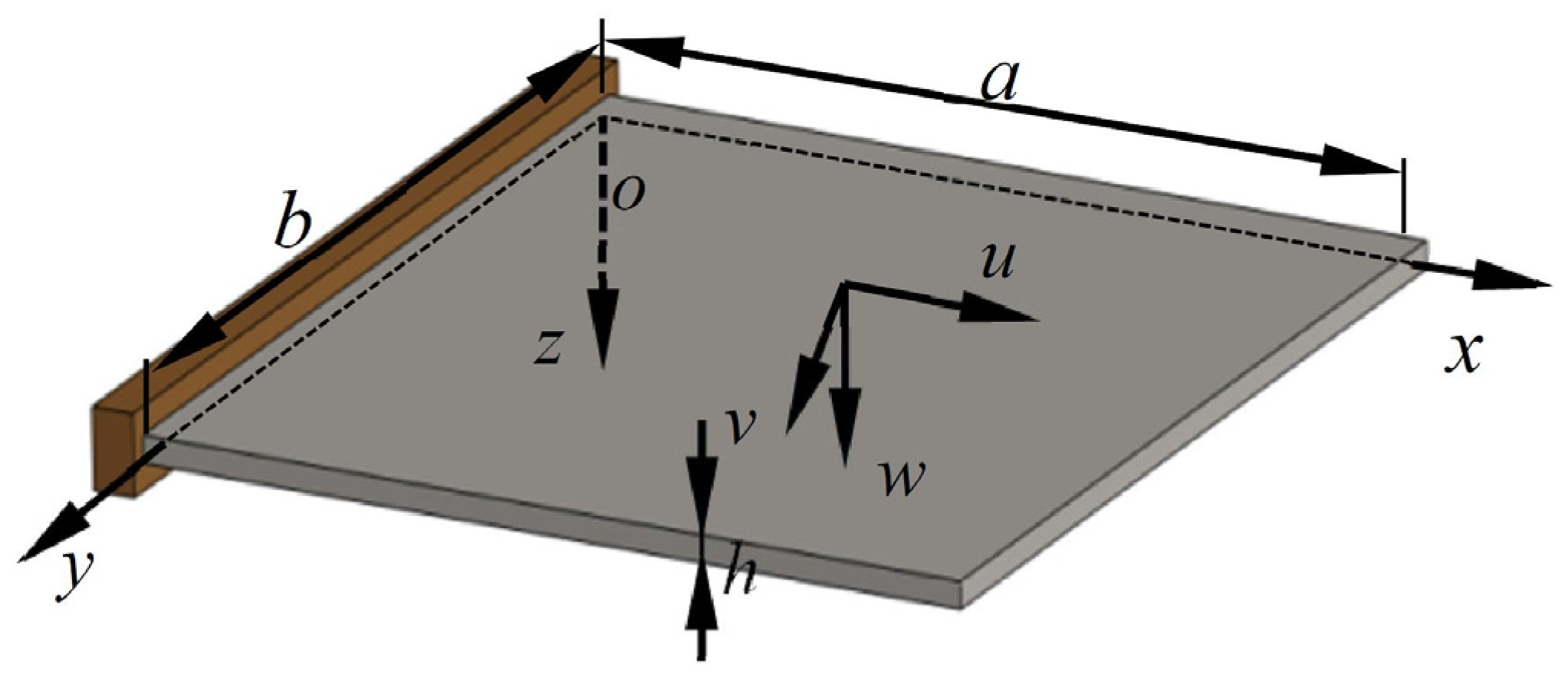
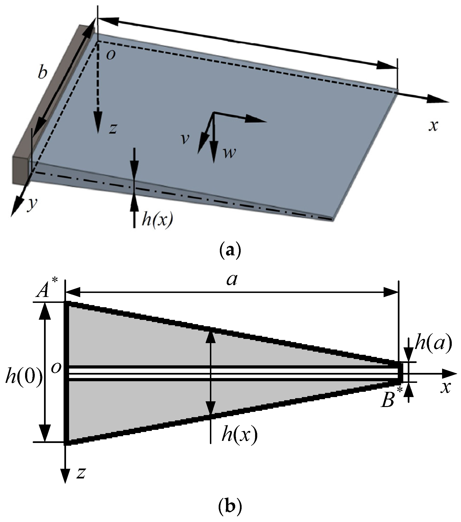
Considering a cantilever plate and the coordinate system $oxyz$, $a$ and $b$ are the length and the width along $x$ and $y$ directions, as shown in Figure 1. $u(x,y,t)$, $v(x,y,t)$ and $w(x,y,t)$ represent the displacement of x, y and z directions, respectively. The Young's modulus, Poisson's ratio and the density of the plate’s material are separately denoted by E, µ and $\mathsf{\rho }$.

The governing equation of the thin plate is [28]

$$D{\nabla }^2{\nabla }^{2}w=\mathsf{\rho }h\frac{{\partial }^{2}w}{\partial t^2},$$

(1)

where ${\nabla }^2$ is the Laplace operator, ${\nabla }^2=\frac{{\partial }^2}{\partial x^2}+\frac{{\partial }^2}{\partial y^2}$.

The cantilever boundary condition can be found in [23] for more details.

Denote the deflection of the plate by using the equation

$$w(x,y,t)=W(x,y)\sin (2\pi \mathsf{\omega }t+\mathsf{\phi }),$$

(2)

where $\mathsf{\omega }$ is the natural frequency of the plate.

Substituting Equation (2) into Equation (1) yields:

$$\frac{{\partial }^{4}W}{\partial x^4}+2\frac{{\partial }^{4}W}{\partial x^2\partial y^2}+\frac{{\partial }^{4}W}{\partial y^4}={\mathsf{\alpha }}^{4}W,$$

(3)

where ${\mathsf{\alpha }}^4={\mathsf{\omega }}^2\frac{\mathsf{\rho }h}{D}$.

Considering that Equation (3) is satisfied by both the model and the prototype:

$$\frac{{\partial }^4{W}_{\mathrm{P}}}{\partial x_{\mathrm{P}}^4}+2\frac{{\partial }^4{W}_{\mathrm{P}}}{\partial x_{\mathrm{P}}^2\partial y_{\mathrm{P}}^2}+\frac{{\partial }^4{W}_{\mathrm{P}}}{\partial y_{\mathrm{P}}^4}={\mathsf{\alpha }}_{\mathrm{P}}^4{W}_{\mathrm{P}},$$

(4a)

$$\frac{{\partial }^4{W}_{\mathrm{m}}}{\partial x_{\mathrm{m}}^4}+2\frac{{\partial }^4{W}_{\mathrm{m}}}{\partial x_{\mathrm{m}}^2\partial y_{\mathrm{m}}^2}+\frac{{\partial }^4{W}_{\mathrm{m}}}{\partial y_{\mathrm{m}}^4}={\mathsf{\alpha }}_{\mathrm{m}}^4{W}_{\mathrm{m}},$$

(4b)

where subscript p represents the prototype; subscript m represents the model, which can be rewritten as

$$\frac{{\mathsf{\lambda }}_W}{{\mathsf{\lambda }}_a^4}\frac{{\partial }^4{W}_{\mathrm{m}}}{\partial x_{\mathrm{m}}^4}+2\frac{{\mathsf{\lambda }}_W}{{\mathsf{\lambda }}_a^2{\mathsf{\lambda }}_b^2}\frac{{\partial }^4{W}_{\mathrm{m}}}{\partial x_{\mathrm{m}}^2\partial y_{\mathrm{m}}^2}+\frac{{\mathsf{\lambda }}_W}{{\mathsf{\lambda }}_b^4}\frac{{\partial }^4{W}_{\mathrm{m}}}{\partial y_{\mathrm{m}}^4}={\mathsf{\lambda }}_{\mathsf{\alpha }}^4{\mathsf{\lambda }}_W{\mathsf{\alpha }}_{\mathrm{m}}^4{W}_{\mathrm{m}},$$

(5)

where ${\mathsf{\lambda }}_j={\mathsf{\lambda }}_{j,\mathrm{p}}/{\mathsf{\lambda }}_{j,\mathrm{m}}$ is used to represent the scaling laws, j represents the symbol of each physical quality, for example, $j=a,b,{\rm E},W$, and so on.

According to the similitude theory [22]:

$$\frac{{\mathsf{\lambda }}_W}{{\mathsf{\lambda }}_a^4}=\frac{{\mathsf{\lambda }}_W}{{\mathsf{\lambda }}_a^2{\mathsf{\lambda }}_b^2}=\frac{{\mathsf{\lambda }}_W}{{\mathsf{\lambda }}_b^4}={\mathsf{\lambda }}_{\mathsf{\alpha }}^4{\mathsf{\lambda }}_W$$

(6)

is obtained from Equation (5), and according to ${\mathsf{\alpha }}^4={\mathsf{\omega }}^2\left(\mathsf{\rho }h/D\right)$ and $D={\rm E}{h}^3/12(1-{\mu }^2)$, there is

$${\mathsf{\lambda }}_{\mathsf{\alpha }}^4={\mathsf{\lambda }}_{\mathsf{\omega }}^2\frac{{\mathsf{\lambda }}_{\mathsf{\rho }}{\mathsf{\lambda }}_h}{{\mathsf{\lambda }}_D}={\mathsf{\lambda }}_{\mathsf{\omega }}^2\frac{{\mathsf{\lambda }}_{\mathsf{\rho }}}{{\mathsf{\lambda }}_h^2{\mathsf{\lambda }}_E}.$$

(7)

Let ${\lambda }_a={\lambda }_b=\lambda$, and

$${\mathsf{\lambda }}_{\mathsf{\omega }}=\sqrt{\frac{{\mathsf{\lambda }}_{\mathsf{{\rm E}}}}{{\mathsf{\lambda }}_{\mathsf{\rho }}}}\frac{{\mathsf{\lambda }}_h}{{\mathsf{\lambda }}^2}$$

(8)

can be derived by substituting Equation (7) into Equation (6), where (8) is the distorted scaling laws with respect to the material parameters and the thickness h.

By using the scaling law (8), the natural frequency of a cantilever thin plate can be predicted by using an MT plate, under the same boundary condition, made of different materials in arbitrary thickness. However, if the prototype is a VT plate, its dynamic properties cannot be predicted by using such a simple scaling law, and an effective approach of designing the scaled down model in predicting the prototype VT plate is needed.

3. Similitude Design of the Variable Thickness (VT) Cantilever Plate

3.1. Simplification of the VT Plate

The cross section of a VT plate with the length and the width of $a$ and $b$, respectively, is shown in Figure 2, where $h(x)$ is the thickness. A Clamped-Free (C-F) boundary condition is satisfied in the present study, the edge $A*$ in Figure 2 is clamped and the edge $B*$ is free.

It is obvious that a VT plate can be simplified as a Stepped Thickness (ST) plate with $q$ steps, where the VT plate and the ST plate are equivalent when $q\to +\infty$, as shown in Figure 3 The thickness of each step is

$$h_{si}=2H_{si}+h(a)(i=1,2,\cdots ,q),$$

(9)

where $H_{si}=\left[2\left(q-i\right)+1\right]\frac{h(0)-h(a)}{2q}$.

For example, consider the VT plate made of 42CrMo, whose geometric and material parameters are shown in

Table 1. Parameters of the variable thickness (VT) plate.

Length a/mm	Width b/mm	Max Thickness $h(0)$/mm	Min Thickness $h(a)$/mm	Young’s Modulus E/Pa	Density $\mathsf{\rho }$/(kg/m3)	Poisson’s Ratio $\mathsf{\mu }$
125	90	6	2	$7\times {10}^{10}$	2770	0.3

, the previous six orders’ natural frequencies, including the flexural vibration (F), the torsional vibration (T) and the chordwise bending vibration (EB), are compared in

Table 3. Comparison between the VT and the ST plates.

Order $i_v$	VT Plate Vibration Model	VT Plate ${\mathsf{\omega }}_v$/Hz	ST Plate Vibration Model	ST Plate ${\mathsf{\omega }}_s$/Hz	Errors ${\mathsf{\eta }}_s$/%
1F	$m=1,n=1$	366.93	$m=1,n=1$	357.25	2.64
1T	$m=2,n=1$	842.42	$m=2,n=1$	830.95	1.36
2F	$m=1,n=2$	1530.40	$m=1,n=2$	1477.70	3.44
2T	$m=2,n=2$	2233.90	$m=2,n=2$	2189.40	1.99
1EB	$m=3,n=1$	2452.70	$m=3,n=1$	2455.40	0.11
3F	$m=1,n=3$	3810.30	$m=1,n=3$	3658.90	3.97

with the simplified ST plate of $q=5$, whose geometric and material parameters are shown in

Table 2. Parameters of the stepped thickness (ST) plate.

Length a/mm	Width b/mm	Young’s Modulus E/Pa	Density $\mathsf{\rho }$ /(kg/m3)	Poisson’s Ratio $\mathsf{\mu }$	Thickness $h_{s1}$/mm	Thickness $h_{s2}$/mm	Thickness $h_{s3}$/mm	Thickness $h_{s4}$/mm	Thickness $h_{s5}$/mm
125	90	$7\times {10}^{10}$	2770	0.3	5.6	4.8	4.0	3.2	2.8

.

The relative simplification error ${\mathsf{\eta }}_s$ between the VT plate and the ST plate is defined as

$${\mathsf{\eta }}_s=\frac{\left|{\mathsf{\omega }}_s-{\mathsf{\omega }}_v\right|}{{\mathsf{\omega }}_v}\times 100\%.$$

(10)

Table 3 indicates that the simplified ST plate has the same vibration modal as the corresponding VT plate. The natural frequency results show small relative errors between the two types of plates as ${\mathsf{\eta }}_s\le 5\%$, especially in the torsional vibration and the chordwise bending vibration, indicating that the equivalent method is applicable.

3.2. Equivalence Design Based on Transfer Matrix

In order to address the issue of predicting the VT cantilever plate by using an MT plate, the transfer matrix method is introduced in this section to establish the equivalent relationship between the ST plate and the thin plate.

3.2.1. Transfer Matrices of the Plate Structures

For a thin walled plate structure, the transfer matrix, which is used to analytically calculate the dynamic properties, can be derived based on the Kirchhoff hypothesis of the thin walled plate element as below.

According to the Hamilton theory [28], the governing equations of the plate element are:

$$\frac{\partial M_x}{\partial x}+\frac{\partial M_{yx}}{\partial y}-Q_x=0,$$

(11a)

$$\frac{\partial M_{xy}}{\partial x}+\frac{\partial M_y}{\partial y}-Q_y=0,$$

(11b)

$$\frac{\partial Q_x}{\partial x}+\frac{\partial Q_y}{\partial y}=\mathsf{\rho }h\frac{{\partial }^{2}w}{\partial t^2},$$

(11c)

where $\mathsf{\rho }h\left({\partial }^{2}w/\partial t^2\right)$ is the inertia term; subscripts x and y represent the directions along x and y axis, respectively. $M_x$, $M_y$ and $M_{xy}$, $M_{yx}$ are denoted as bending and twisting moments as:

$$\begin{array}{l}{M}_x=-D\left(\frac{{\partial }^{2}w}{\partial x^2}+\mathsf{\mu }\frac{{\partial }^{2}w}{\partial y^2}\right)\\ M_y=-D\left(\frac{{\partial }^{2}w}{\partial y^2}+\mathsf{\mu }\frac{{\partial }^{2}w}{\partial x^2}\right)\\ M_{xy}=M_{yx}=-D\left(1-\mathsf{\mu }\right)\frac{{\partial }^{2}w}{\partial x\partial y}\end{array},$$

(12)

respectively, where $D=E{h}^3/12(1-{\mathsf{\mu }}^2)$ represents the flexural rigidity of the plate element.

Furthermore, an equation of the rotation angle ${\mathsf{\theta }}_x$, which is related to the boundary conditions, is introduced as

$${\mathsf{\theta }}_x=-\frac{\partial w}{\partial x},$$

(13)

such that seven equations are established with seven variables of $\left\{w{\mathsf{\theta }}_x{M}_x{M}_y{M}_{xy}{Q}_x{Q}_y\right\}$.

According to governing Equations (11) to (13), denote the variable vector as:

$$\mathit{P}\left(x,y,t\right)={\left[\begin{array}{ccccccc}w& {\mathsf{\theta }}_x& M_x& M_y& M_{xy}& Q_x& Q_y\end{array}\right]}^{\mathrm{T}},$$

(14)

such that Equations (11) to (13) can be written into a matrix form as

$$\frac{\partial \mathit{P}(x,y,t)}{\partial x}=\mathit{U}\mathit{P}(x,y,t),$$

(15)

where $\mathit{U}$ is a 7 × 7 matrix given by

$$\mathit{U}=\left[\begin{array}{ccccccc}0& U_{12}& 0& 0& 0& 0& 0\\ U_{21}& 0& U_{23}& 0& 0& 0& 0\\ 0& 0& 0& 0& U_{35}& U_{36}& 0\\ 0& U_{42}& 0& 0& U_{45}& U_{46}& 0\\ 0& 0& 0& U_{54}& 0& 0& U_{57}\\ U_{61}& 0& 0& 0& 0& 0& U_{67}\\ 0& U_{72}& 0& 0& U_{75}& U_{76}& 0\end{array}\right],$$

(16)

with $U_{12}=-1$; $U_{21}=\mu \frac{{\partial }^2}{\partial y^2}$; $U_{23}=\frac{12(1-{\mathsf{\mu }}^2)}{E{h}^3}$; $U_{35}=-\frac{\partial }{\partial y}$; $U_{36}=1$; $U_{42}=\frac{E{h}^3}{12}\frac{{\partial }^2}{\partial y^2}$; $U_{45}=-\mathsf{\mu }\frac{\partial }{\partial y}$; $U_{46}=\mathsf{\mu }$; $U_{54}=-\frac{\partial }{\partial y}$; $U_{57}=1$; $U_{61}=\mathsf{\rho }h\frac{{\partial }^2}{\partial t^2}$; $U_{67}=-\frac{\partial }{\partial y}$; $U_{72}=\frac{E{h}^3}{12(1+\mathsf{\mu })}\frac{{\partial }^3}{\partial y^3}$; $U_{75}=-\frac{{\partial }^2}{\partial y^2}$; and $U_{76}=\frac{\partial }{\partial y}$.

It is worth noting that the transfer matrix of the flexural vibration can be established by using the one-dimensional method, meaning only two boundary conditions are considered ($x=0$ and $x=a$), to lead a much simpler form than the other two vibration modals (T and EB). Consequently, the flexural vibration is taken as an example in the following work. The other two types of vibrations can be discussed through the same process, and their transfer matrices are shown in references [25,29].

In a flexural vibration, the displacement functions and the corresponding stresses are assumed as follows:

$$\mathit{P}\left(x,y,t\right)=\left[\begin{array}{c}\tilde{w}\left(x\right)\sin \left(my\right)\\ {\tilde{\mathsf{\theta }}}_x\left(x\right)\sin \left(my\right)\\ {\tilde{M}}_x\left(x\right)\sin \left(my\right)\\ {\tilde{M}}_y\left(x\right)\sin \left(my\right)\\ {\tilde{M}}_{xy}\left(x\right)\cos \left(my\right)\\ {\tilde{Q}}_x\left(x\right)\cos \left(my\right)\\ {\tilde{Q}}_y\left(x\right)\cos \left(my\right)\end{array}\right]{\mathrm{e}}^{\mathrm{j}\mathsf{\omega }t},$$

(17)

where denotation of the wave number along the $y$ direction is $m=1$, and $\{\tilde{w}\left(x\right){\tilde{\mathsf{\theta }}}_x\left(x\right){\tilde{M}}_x\left(x\right){\tilde{M}}_y\left(x\right)$ ${\tilde{M}}_{xy}\left(x\right){\tilde{Q}}_x\left(x\right){\tilde{Q}}_y\left(x\right)\}$ are undefined functions only related to $x$.

Substituting Equation (17) into Equation (15) yields:

$$\frac{\mathrm{d}\tilde{\mathit{P}}(x)}{\mathrm{d}x}=\tilde{\mathit{U}}\tilde{\mathit{P}}(x),$$

(18)

where

$$\tilde{\mathit{P}}\left(x\right)={\left[\begin{array}{ccccccc}\tilde{w}& {\tilde{\mathsf{\theta }}}_x& {\tilde{M}}_x& {\tilde{M}}_y& {\tilde{M}}_{xy}& {\tilde{Q}}_x& {\tilde{Q}}_y\end{array}\right]}^{\mathrm{T}},$$

(19)

and

$$\tilde{\mathit{U}}=\left[\begin{array}{ccccccc}0& {\tilde{U}}_{12}& 0& 0& 0& 0& 0\\ {\tilde{U}}_{21}& 0& {\tilde{U}}_{23}& 0& 0& 0& 0\\ 0& 0& 0& 0& {\tilde{U}}_{35}& {\tilde{U}}_{36}& 0\\ 0& {\tilde{U}}_{42}& 0& 0& {\tilde{U}}_{45}& {\tilde{U}}_{46}& 0\\ 0& 0& 0& {\tilde{U}}_{54}& 0& 0& {\tilde{U}}_{57}\\ {\tilde{U}}_{61}& 0& 0& 0& 0& 0& {\tilde{U}}_{67}\\ 0& {\tilde{U}}_{72}& 0& 0& {\tilde{U}}_{75}& {\tilde{U}}_{76}& 0\end{array}\right],$$

(20)

where ${\tilde{U}}_{12}=-1$; ${\tilde{U}}_{21}=-m^2\mathsf{\mu }$; ${\tilde{U}}_{23}=\frac{12(1-{\mathsf{\mu }}^2)}{E{h}^3}$; ${\tilde{U}}_{35}=m$; ${\tilde{U}}_{36}=1$; ${\tilde{U}}_{42}=-\frac{E{h}^3}{12}{m}^2$; ${\tilde{U}}_{45}=m\mathsf{\mu }$; ${\tilde{U}}_{46}=\mathsf{\mu }$; ${\tilde{U}}_{54}=-m$; ${\tilde{U}}_{57}=1$; ${\tilde{U}}_{61}=-\mathsf{\rho }h{\mathsf{\omega }}^2$; ${\tilde{U}}_{67}=m$; ${\tilde{U}}_{72}=-m^3\frac{E{h}^3}{12(1+\mathsf{\mu })}$; ${\tilde{U}}_{75}=m^2$; ${\tilde{U}}_{76}=-m$, and $m=1$.

Considering that the thin plate is divided into $K$ sub-sections along the $x$ direction, for the $k$th sub-section, the solution of (18) can be written as [30]

$$\tilde{\mathit{P}}(a_k)=\mathit{T}(a_k)\tilde{\mathit{P}}\left(a_{k-1}\right),$$

(21)

where $a_k$ is the length of the $k$th sub-section, and $\mathit{T}(a_k)={\mathrm{e}}^{\left(\tilde{\mathit{U}}{a}_k\right)}$ is the transfer matrix of the plate element.

By combining Eqution (21) along the length of the plate, there is

$$\tilde{\mathit{P}}\left(a\right)={\mathit{T}}_{th}\tilde{\mathit{P}}\left(0\right),$$

(22)

where $T_{th}={\displaystyle \prod _{k=1}^K{e}^{\tilde{\mathit{U}}{a}_k}}=e^{\tilde{\mathit{U}}a}$ is the transfer matrix of the thin plate.

3.2.2. Equivalent Thickness of the Thin Plate

Assume that the simplified ST plate contains $N$ steps with each length of $a_{s{i}_0}$ and the thickness of $h_{s{i}_0}$ $(i_0=1,2,\cdots ,N)$, as shown in Figure 4.

Each step of the plate, by applying the transfer matrix method, can be divided into $r$ sections, such that, in total, $R=N\times r$ subsections are applied in analyzing the ST plate, where the boundary of each section is defined as ${\mathsf{\xi }}_i$, $(i=0,1,\cdots ,R)$.

For the ST plate, Equation (22) can be written as:

$${\left[\begin{array}{c}\tilde{w}\\ {\tilde{\mathsf{\theta }}}_x\\ {\tilde{M}}_x\\ {\tilde{M}}_y\\ {\tilde{M}}_{xy}\\ {\tilde{Q}}_x\\ {\tilde{Q}}_y\end{array}\right]}_{{\mathsf{\xi }}_{\left(n-1\right)r}}={\left[\begin{array}{ccccccc}{T}_{11}& T_{12}& T_{13}& T_{14}& T_{15}& T_{16}& T_{17}\\ T_{21}& T_{22}& T_{23}& T_{24}& T_{25}& T_{26}& T_{27}\\ T_{31}& T_{32}& T_{33}& T_{34}& T_{35}& T_{36}& T_{37}\\ T_{41}& T_{42}& T_{43}& T_{44}& T_{45}& T_{46}& T_{47}\\ T_{51}& T_{52}& T_{53}& T_{54}& T_{55}& T_{56}& T_{57}\\ T_{61}& T_{62}& T_{63}& T_{64}& T_{65}& T_{66}& T_{67}\\ T_{71}& T_{72}& T_{73}& T_{74}& T_{75}& T_{76}& T_{77}\end{array}\right]}_n{\left[\begin{array}{c}\tilde{w}\\ {\tilde{\mathsf{\theta }}}_x\\ {\tilde{M}}_x\\ {\tilde{M}}_y\\ {\tilde{M}}_{xy}\\ {\tilde{Q}}_x\\ {\tilde{Q}}_y\end{array}\right]}_{{\mathsf{\xi }}_{nr}}$$

(23)

for the $n$ th step, where $T_{ij}(i=1,2,\cdots ,7;j=1,2,\cdots ,7)$ are the elements of the transfer matrix.

According to Equation (21), the $n$ th transfer matrix in (23) is calculated as:

$${\mathit{T}}_n={\mathrm{e}}^{\left({\tilde{\mathit{U}}}_n{a}_{sn}\right)},$$

(24)

where

$${\mathit{T}}_n={\left[\begin{array}{ccccccc}{T}_{11}& T_{12}& T_{13}& T_{14}& T_{15}& T_{16}& T_{17}\\ T_{21}& T_{22}& T_{23}& T_{24}& T_{25}& T_{26}& T_{27}\\ T_{31}& T_{32}& T_{33}& T_{34}& T_{35}& T_{36}& T_{37}\\ T_{41}& T_{42}& T_{43}& T_{44}& T_{45}& T_{46}& T_{47}\\ T_{51}& T_{52}& T_{53}& T_{54}& T_{55}& T_{56}& T_{57}\\ T_{61}& T_{62}& T_{63}& T_{64}& T_{65}& T_{66}& T_{67}\\ T_{71}& T_{72}& T_{73}& T_{74}& T_{75}& T_{76}& T_{77}\end{array}\right]}_n.$$

Combining all $N$ steps of the ST plate by using the transfer matrix (23) yields

$${\left[\begin{array}{c}\tilde{w}\\ {\tilde{\mathsf{\theta }}}_x\\ {\tilde{M}}_x\\ {\tilde{M}}_y\\ {\tilde{M}}_{xy}\\ {\tilde{Q}}_x\\ {\tilde{Q}}_y\end{array}\right]}_0={\displaystyle \prod _{n=1}^N{\mathit{T}}_n}{\left[\begin{array}{c}\tilde{w}\\ {\tilde{\mathsf{\theta }}}_x\\ {\tilde{M}}_x\\ {\tilde{M}}_y\\ {\tilde{M}}_{xy}\\ {\tilde{Q}}_x\\ {\tilde{Q}}_y\end{array}\right]}_{Nr}={\displaystyle \prod _{n=1}^N{\mathrm{e}}^{\left({\tilde{\mathit{U}}}_n{a}_{sn}\right)}}{\left[\begin{array}{c}\tilde{w}\\ {\tilde{\mathsf{\theta }}}_x\\ {\tilde{M}}_x\\ {\tilde{M}}_y\\ {\tilde{M}}_{xy}\\ {\tilde{Q}}_x\\ {\tilde{Q}}_y\end{array}\right]}_{Nr},$$

(25)

where $\overline{\mathit{T}}={\displaystyle \prod _{n=1}^N{\mathrm{e}}^{\left({\tilde{\mathit{U}}}_n{a}_{sn}\right)}}$ represents the transfer matrix of the ST plate.

Substituting the boundary condition of the cantilever plate,

$$\tilde{w}={\tilde{\mathsf{\theta }}}_x=0\text{ for }x=0,$$

(26a)

and

$${\tilde{M}}_x={\tilde{M}}_y={\tilde{M}}_{xy}={\tilde{Q}}_x={\tilde{Q}}_y=0\text{ for }x=a$$

(26b)

into Equation (25), yields

$${\left[\begin{array}{c}0\\ 0\end{array}\right]}_0=\left[\begin{array}{cc}{\overline{T}}_{11}& {\overline{T}}_{12}\\ {\overline{T}}_{21}& {\overline{T}}_{22}\end{array}\right]{\left[\begin{array}{c}\tilde{w}\\ {\tilde{\mathsf{\theta }}}_x\end{array}\right]}_{Nr},$$

(27)

where ${\overline{T}}_{ij}$ are the elements of the transfer matrix $\overline{\mathit{T}}$.

According to Equation (27), the natural frequency of the ST plate can be obtained by letting

$$\det \left(\left[\begin{array}{cc}{\overline{T}}_{11}& {\overline{T}}_{12}\\ {\overline{T}}_{21}& {\overline{T}}_{22}\end{array}\right]\right)=0.$$

(28)

The specific algorithm of calculating Equation (28) is discussed in [19] in details.

Similarly, the natural frequency of a thin plate can be calculated as

$$\det \left(\left[\begin{array}{cc}{T}_{th11}& T_{th12}\\ T_{th21}& T_{th22}\end{array}\right]\right)=0.$$

(29)

In Equation (28), each order’s natural frequencies of the ST plate’s flexural vibration, defined as ${\mathsf{\omega }}_{st,n}$, are obtained by ordering the results in a small to large array. Consequently, Equation (28) can be expressed as

$$\overline{T}({\mathsf{\omega }}_{st,n})={\displaystyle \prod _{n=1}^N{\mathrm{e}}^{{\tilde{\mathit{U}}}_n{a}_{sn}}}=0,$$

(30)

While, for an equivalent thin plate, the equivalent thickness corresponding to each order’s vibration, $h_{e,n}$, is the variable need to be obtained, and Equation (29) is

$$T_{th}(h_{e,n})={\mathrm{e}}^{\tilde{\mathit{U}}a}=0,$$

(31)

where the frequency ${\mathsf{\omega }}_{st}$ calculated by Equation (30) is substituted into Equation (31).

Consequently, the equivalent thickness of the thin plate to an ST plate is obtained.

4. The Distorted Model of the VT Plate

4.1. Distorted Models and the Scaling Law

It has been discussed in the previous sections that for each vibration modal, an equivalent thickness of a VT plate can be calculated as $h_{e,n}$ via the simplified ST plate by using the transfer matrix method. However, in practice, it is obviously impossible to design an MT plate with a specific thickness $h_{e,n}$ for each modal of the prototype VT plate. Usually, a unified thickness, $h_{Uni}$, is chosen in the design of the scaled model.

In order to address this issue, denote the ration of the thickness as

$$\Xi =\frac{h_{e,n}}{h_{Uni}}.$$

(32)

According to the frequency scaling law (8), the frequency relationship between the prototype equivalent thin plate and its scaled down model is

$${\mathsf{\lambda }}_{\mathsf{\omega },\mathrm{p}-\mathrm{m}}=\sqrt{\frac{{\mathsf{\lambda }}_E}{{\mathsf{\lambda }}_{\mathsf{\rho }}}}\frac{{\mathsf{\lambda }}_{h_e}}{{\mathsf{\lambda }}^2},$$

(33)

while the scaling law between the scaled model thin plate and the distorted model plate with the unified thickness h_Uni is calculated as

$${\mathsf{\lambda }}_{\mathsf{\omega },\mathrm{m}-\mathrm{u}}=\frac{h_{\left(e,n\right),\mathrm{m}}}{h_{Uni}}=\Xi {\mathsf{\lambda }}_{h_e},$$

(34)

where $h_{\left(e,n\right),\mathrm{m}}$ represents the model thickness against the $n$th modal of the thin plate.

Consequently, the scaling law between the unified distorted model and the prototype equivalent thin plate, as well as the VT plate, is derived as

$${\mathsf{\lambda }}_{\mathsf{\omega }}={\mathsf{\lambda }}_{\mathsf{\omega },\mathrm{p}-\mathrm{m}}{\mathsf{\lambda }}_{\mathsf{\omega },\mathrm{m}-\mathrm{u}}=\sqrt{\frac{{\mathsf{\lambda }}_E}{{\mathsf{\lambda }}_{\rho }}}\frac{{\mathsf{\lambda }}_{h_e}}{{\mathsf{\lambda }}^2}\Xi {\mathsf{\lambda }}_{h_e}=\sqrt{\frac{{\mathsf{\lambda }}_E}{{\mathsf{\lambda }}_{\rho }}}\Xi ,$$

(35)

when ${\mathsf{\lambda }}_a={\mathsf{\lambda }}_b={\mathsf{\lambda }}_{h_e}=\mathsf{\lambda }$.

Next, a similitude design case study is provided to illustrate the design process of the scaled down plate. In this case study, the simplified steps of the ST plate are given as $N=5$, and the material and the geometrical parameters are shown in Table 2, where in the ANSYS simulation (ANSYS 14.0, ANSYS, Pittsburgh, PA, USA), the element Solid 186 is used. The equivalent thickness of the previous fourth flexural vibration modal defined as $h_{eiF},i=1,\dots ,4$, and the relative prediction error is calculated by

$${\mathsf{\eta }}_e=\frac{\left|{\mathsf{\omega }}_e-{\mathsf{\omega }}_s\right|}{{\mathsf{\omega }}_s}\times 100\%,$$

(36)

as shown in

Table 4. Different orders’ equivalent thickness.

Vibration Mode	Equivalent Thickness /mm	ST Plate 1 ANSYS ${\mathsf{\omega }}_s$/Hz	Thin plate ANSYS ${\mathsf{\omega }}_e$/Hz	Error ${\mathsf{\eta }}_e$/%
$m=1,n=1$	$h_{e1F}=6.57$	357.25	355.76	0.42
$m=1,n=2$	$h_{e2F}=4.45$	1477.70	1470.60	0.48
$m=1,n=3$	$h_{e3F}=3.95$	3658.90	3689.51	0.84
$m=1,n=4$	$h_{e4F}=3.77$	6894.76	6814.79	1.16

¹ ST plate represents the stepped thickness plate.

, where the width, length and material parameters of the equivalent thin plate are the same as the ST plate as shown in Table 2, and ${\mathsf{\omega }}_e$ and ${\mathsf{\omega }}_s$ are the natural frequencies of the equivalent thickness thin plate and the ST plate, respectively.

The results in Table 4 show that the ST plate has the same order and shape of the vibration modal as the equivalent thin plate, and the natural frequencies of each order’s vibration are also close to a small relative error of ${\mathsf{\eta }}_e<2\%$. This indicates that the design algorithm on calculating the equivalent thickness is applicable, and, therefore, the connections between the VT plate, ST plate and the thin plate are established.

Consider that, in a scaled down model, the material of the model plate is NO. 45 steel and the geometrical parameters of the plate are shown in

Table 5. Parameters of the model thin (MT) plate.

Type of the Plate	Length a/mm	Width b/mm	Thickness h/mm	Young’s Modulus E/Pa	Density $\mathsf{\rho }$/(kg/m3)	Poisson’s Ratio $\mathsf{\mu }$
Model	62.5	45	1	$2\times {10}^{11}$	7850	0.3

with $\mathsf{\lambda }=2$. The unified thickness of the model plate is $h_{Uni}=2\text{\hspace{0.17em}mm}$, and the predicted natural frequencies obtained by using the scaling law (35) are shown in

Table 6. Prediction of the VT plate.

Vibration Model	VT 2 Plate ${\mathsf{\omega }}_s$/Hz	MT 2 Plate ${\mathsf{\omega }}_{\mathrm{m}}$/Hz	$\Xi =\frac{{\mathsf{\lambda }}_h}{\mathsf{\lambda }}$	Predicted Frequencies ${\mathsf{\omega }}_{pr}$/Hz	Error ${\mathsf{\eta }}_{ave}$/%
$m=1,n=1$	366.93	215.131	3.285	351.94	4.09
$m=1,n=2$	1530.40	1334.22	2.225	1478.38	3.40
$m=1,n=3$	3610.30	3790.03	1.975	3727.68	3.25
$m=1,n=4$	7080.52	7382.59	1.885	6930.25	2.12

² VT plate represents the variable thickness plate; MT plate represents the model thin plate.

, where ${\mathsf{\eta }}_{ave}$ is the relative error of predictive values.

Table 6 shows accurate predicted results that in the same vibration modal, the predicted natural frequencies are close to that of the prototype with a relative error ${\mathsf{\eta }}_{ave}<5\%$, indicating that the method of predicting a VT plate’s vibration characteristics by using an MT plate is applicable.

In this example, it can be seen that the dynamic properties of a VT plate can be accurately predicted by using a designed MT plate of different materials. It is worth noting that the present proposed method can be simply achieved by using the MATLAB program (MATLAB 2010b, MathWorks, Natick, MA, USA), such that the design of the MT plate can be easily conducted. Moreover, two additional cases are discussed as below.

Firstly, only flexible vibration is considered in the proposed example. It is noticeable that the coefficient $\Xi$ of the torsional vibration and the chordwise bending vibration can be obtained by replacing $\mathit{T}$ with transfer matrices shown in Reference [29].

Secondly, the length and width of the MT plate are completely scaled down as ${\mathsf{\lambda }}_a={\mathsf{\lambda }}_b=\mathsf{\lambda }$, a more complex case, where the geometric parameters are all distorted as ${\mathsf{\lambda }}_a\ne {\mathsf{\lambda }}_b\ne {\mathsf{\lambda }}_{h_e}$, can be discussed by using the similar process by referring to the scaling laws present in [22,23,24] between the equivalent thin plate and the MT plate.

4.2. A General Design Process

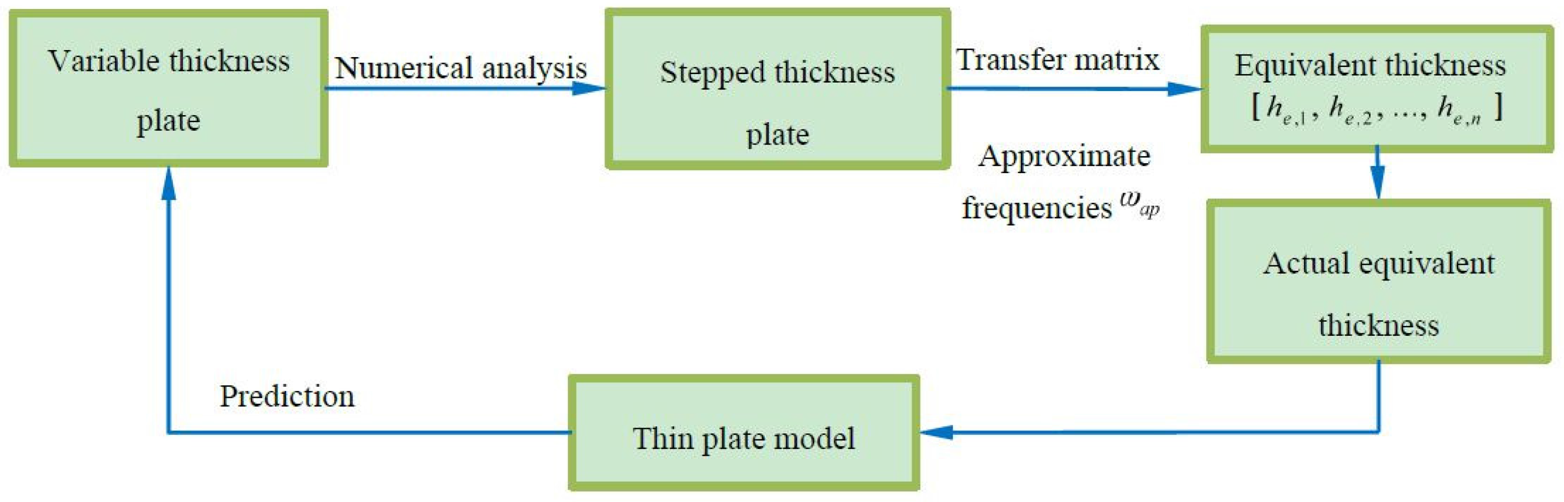
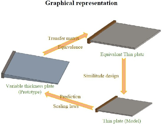
According to the discussion in the above sections, a distorted scaled model of the VT plate is designed and the method of reducing the predicted errors is investigated. To be clear, the process of the similitude design is summarized as below and illustrated in Figure 5.

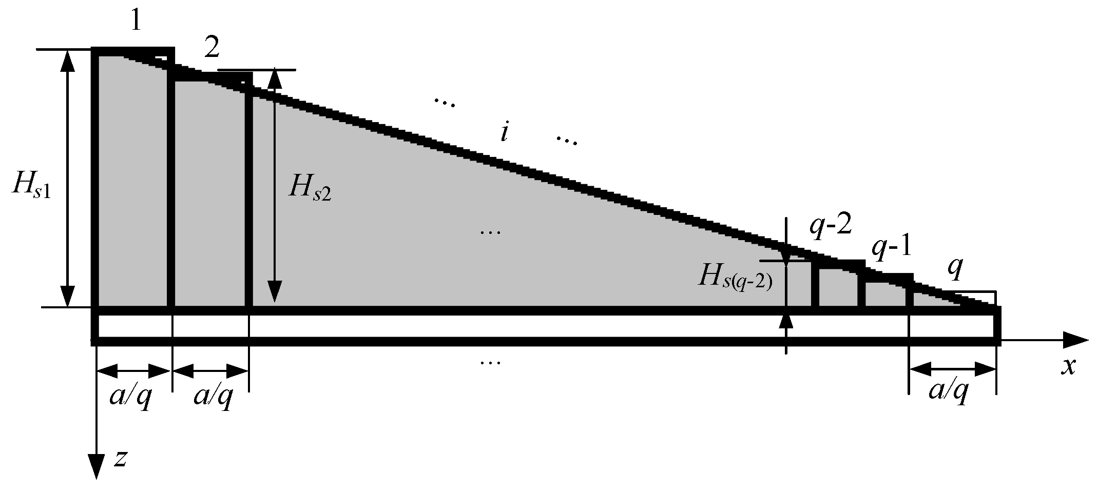
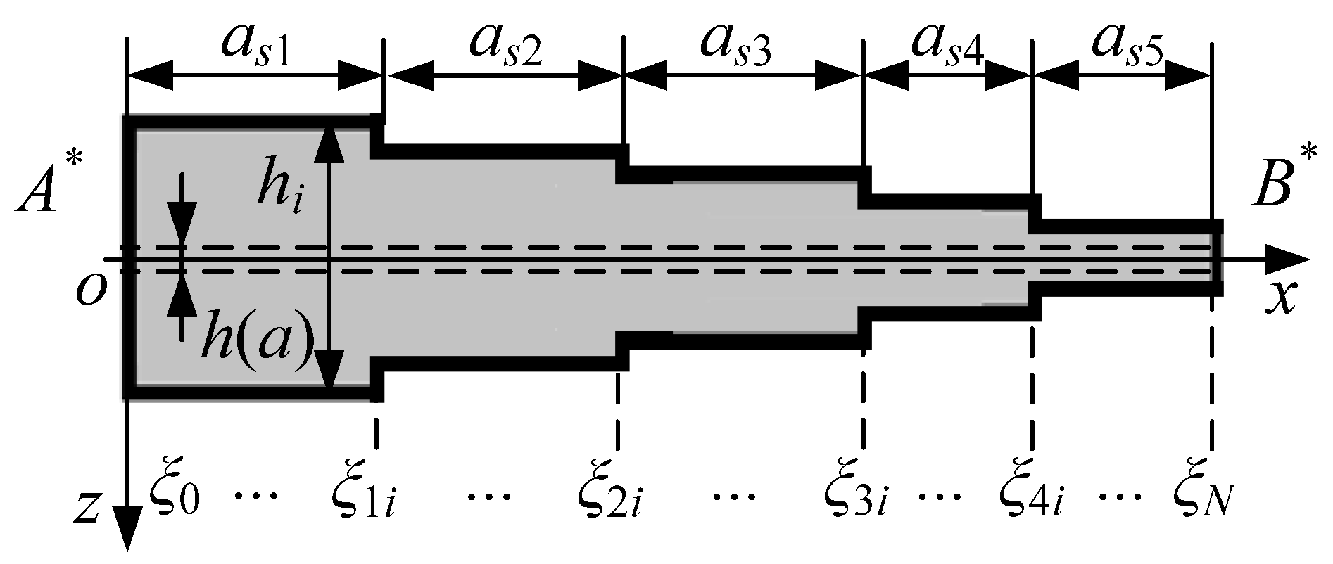
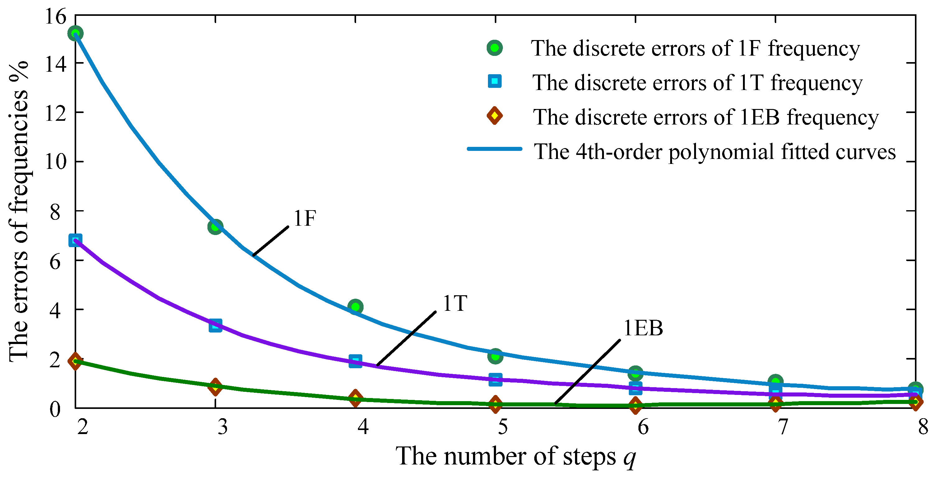
Step 1: Simplify the VT plate by using an ST plate with finite steps $N$, such that the simplified ST plate can reveal the dynamic properties of the VT plate in a certain order.

Usually, this process can be facilitated by using a numerical analysis method. For example, in the case study of this paper, the frequency errors of different vibration modals between the VT plate and the ST plate with different $N$ steps are shown in Figure 6.

Fitting the curves with a four-order polynomials yields:

$$\{\begin{array}{l}{\mathsf{\eta }}_{s,1F}=2.826\times {10}^{-4}{N}^4-7.175\times {10}^{-3}{N}^3+6.908\times {10}^{-2}{N}^2-0.3043N+0.537\\ {\mathsf{\eta }}_{s,1T}=1.578\times {10}^{-4}{N}^4-3.825\times {10}^{-3}{N}^3+3.51\times {10}^{-2}{N}^2-0.1474N+0.2505\\ {\mathsf{\eta }}_{s,1EB}=2.199\times {10}^{-5}{N}^4-6.265\times {10}^{-4}{N}^3+6.93\times {10}^{-3}{N}^2-3.436\times {10}^{-2}N+6.448\times {10}^{-2}\end{array},$$

(37)

where the adjusted determination coefficient $R^2$ is given as:

$$R^2=1-\left[\frac{n^{\prime }-1}{n^{\prime }-(k+1)}\right]\left(1-\frac{{\displaystyle \sum {\left({\widehat{Y}}_i-\overline{Y}\right)}^2}}{{\displaystyle \sum {\left(Y_i-\overline{Y}\right)}^2}}\right)(i=1,2,\cdots ,n^{\prime }),$$

(38)

where $n^{\prime }$ is the sample size; $k$ is the order of the polynomial; $\widehat{Y}$, $\overline{Y}$ and $Y$ are the fitted value, the average value and the actual value (simulation value), respectively.

Substituting relevant parameters into Equation (38) yields:

$${R^2}_{1F}=0.9995,{R^2}_{1T}=0.9846,{R^2}_{1EB}=0.9928$$

(39)

where Equation (39) indicates that the fitted curves can be used to determine ${\mathsf{\eta }}_{s,1F},{\mathsf{\eta }}_{s,1T}$ and ${\mathsf{\eta }}_{s,1EB}$.

Assuming ${\mathsf{\eta }}_s\le 5\%$ is acceptable, the step number $N$ is solved: $N=4$. Similarly, calculating the frequency errors of high order vibrations (previous six modals), $N=5$ is chosen as the number of the steps in the case study.

Step 2: Calculate the equivalent thickness of each order’s vibration by using the transfer matrix method, which is obtained as $h_{e,1},h_{e,2},\mathrm{...},h_{e,n}$.

Step 3: Unify the equivalent thickness obtained in Step 2 into any thickness of interest as $h_{Uni}$, and design the similitude model of the thin plate with the thickness $h_{Uni}$.

Step 4: Derive the distorted scaling laws (35) according to the equivalent thickness $h_{e,1},h_{e,2},\mathrm{...},h_{e,n}$ and the simplified thickness , as well as the different materials of the model and the prototype.

Step 5: Test the distorted model and predict the dynamic characteristics of the prototype VT plate.

It is worth noting that the design process summarized above is a general process on designing a distorted similitude model of thin walled structures with continuous thickness variations. Based on the sketch shown in Figure 5, two main issues are addressed in the present study. Firstly, find a simple equivalent structure that has the same dynamic properties of interest to the prototype complex structure. Then, design the similitude model of the simple equivalent structure according to the requirement of the designer, where, in this step, dynamic similitude design approaches that have been studied by the authors can be well applied. The proposed technique in the present study can be extended to dealing with, i.e., thin walled shells, annular plates, etc. that have the characteristic of variable thickness.

5. Conclusions

Much research has been done on the similitude design of thin walled structures, such as plates and cylindrical shells. However, in engineering practice, the real structures do not always have the same thickness characteristic. The variable thickness can significantly affect the dynamic properties of the structure such that the prediction of the simple scaled down model may fail in its accuracy.

In order to address this issue, a new technique for the similitude design of a cantilever VT plate is proposed in the present study based on the transfer matrix method. In this approach, a simplified ST plate is introduced as a connection between the VT plate and the equivalent thin plate, such that the distorted similitude design method of the thin walled structure can be directly applied in designing the scaled model. The transfer matrices of the ST plate and the thin plate have been derived in this study, and the equivalent thickness $h_{e,n}$ of the thin plate corresponding to the specific vibration modal of the VT plate are calculated according to these transfer matrices. Moreover, a unified model plate is defined as the Model Thin (MT) plate such that different orders’ dynamic properties of the prototype VT plate can be predicted by using only one scaled model with the thickness $h_{Uni}$, and the scaling law between the scaled model and the prototype are also derived as (35). Finally, a case study is employed to validate the proposed approach in the present study, and a general process of determining the scaled model and its scaling laws are summarized to emphasis its significance in engineering practice.

References

1. Luo, Z.; Zhao, X.Y.; Zhu, Y.P.; Wang, D.Y. Determination method of the structure size interval of dynamic similar models for predicting vibration characteristics of the isotropic sandwich plates. J. Vibroeng. 2013, 15, 1728–1743. [Google Scholar]
2. Yao, M.H.; Chen, Y.P.; Zhang, W. Nonlinear vibrations of blade with varying rotating speed. Nonlinear Dyn. 2012, 68, 487–504. [Google Scholar] [CrossRef]
3. Qin, Z.Y.; Han, Q.K.; Chu, F.L. Analytical model of bolted disk-drum joints and its application to dynamic analysis of jointed rotor. J. Mech. Eng. Sci. 2014, 228, 646–663. [Google Scholar] [CrossRef]
4. Yao, M.H.; Zhang, W. Using the extended Melnikov method to study multi-pulse chaotic motions of a rectangular thin plate. Int. J. Dyn. Control. 2014, 2, 365–385. [Google Scholar] [CrossRef]
5. Rand, O. Experimental study of the natural frequencies of rotating thin-walled composite blades. Thin Wall Struct. 1995, 21, 191–207. [Google Scholar] [CrossRef]
6. Yang, X.D.; Zhang, W.; Chen, L.Q.; Yao, M.H. Dynamical analysis of axially moving plate by finite difference method. Nonlinear Dyn. 2012, 67, 997–1006. [Google Scholar] [CrossRef]
7. Huang, M.; Ma, X.Q.; Sakiyama, T.; Matuda, H.; Morita, C. Free vibration analysis of orthotropic rectangular plates with variable thickness and general boundary conditions. J. Sound Vib. 2005, 288, 931–955. [Google Scholar] [CrossRef]
8. Sakiyama, T.; Huang, M. Free vibration analysis of rectangular plates with variable thickness. J. Sound Vib. 1998, 216, 379–397. [Google Scholar] [CrossRef]
9. Guo, S.J.; Keane, A.J.; Moshrefi-Torbati, M. Vibration analysis of stepped thickness plates. J. Sound Vib. 1997, 204, 645–657. [Google Scholar]
10. Eisenberger, M.; Jabareen, M. Axisymmetric vibrations of circular and annular plates with variable thickness. Int. J. Struct. Stab. Dyn. 2001, 1, 195–206. [Google Scholar] [CrossRef]
11. Jiang, W.; Redekop, D. Static and vibration analysis of orthotropic toroidal shells of variable thickness by differential quadrature. Thin Wall Struct. 2003, 41, 461–478. [Google Scholar] [CrossRef]
12. Kang, J.H.; Leissa, A.W. Free vibration analysis of complete paraboloidal shells of revolution with variable thickness and solid paraboloids from a three-dimensional theory. Comput. Struct. 2005, 83, 2594–2608. [Google Scholar] [CrossRef]
13. Shufrin, I.; Eisenberger, M. Vibration of shear deformable plates with variable thickness—first-order and higher-order analyses. J. Sound Vib. 2006, 290, 465–489. [Google Scholar] [CrossRef]
14. Bacciocchi, M.; Eisenberger, M.; Fantuzzi, N.; Tornabene, F.; Viola, E. Vibration analysis of variable thickness plates and shells by the generalized differential quadrature method. Comput. Struct. 2016. [Google Scholar] [CrossRef]
15. Tornabene, F.; Fantuzzi, N.; Bacciocchi, M. The local GDQ method for the natural frequencies of doubly-curved shells with variable thickness: a general formulation. Engineering 2016, 92, 265–289. [Google Scholar] [CrossRef]
16. Sriniviasan, A.V. Flutter and resonant vibration characteristics of engine blades. J. Eng. Gas Turb. Power 1997, 119, 742–775. [Google Scholar] [CrossRef]
17. Sun, J.; Kari, L.; Lopez Arteaga, I. A dynamic rotating blade model at an arbitrary stagger angle based on classical plate theory and the Hamilton’s principle. J. Sound Vib. 2013, 332, 1355–1371. [Google Scholar] [CrossRef]
18. De Rosa, S.; Franco, F.; Meruane, V. Similitudes for the structural response of flexural plates. J. Mech. Eng. Sci. 2016, 230, 2174–2188. [Google Scholar] [CrossRef]
19. Ramu, M.; Raja, V.P.; Thyla, P.R. Establishment of structural similitude for elastic models and validation of scaling laws. KSCE J. Civ. Eng. 2013, 17, 139–144. [Google Scholar]
20. Qian, Y.; Swanson, S.R.; Nuismer, R.J.; Bucinell, R.B. An experimental study of scaling rules for impact damage in fiber composites. J. Compos. Mater. 1990, 24, 559–570. [Google Scholar] [CrossRef]
21. Ungbhakorn, V.; Singhatanadgid, P. Similitude invariants and scaling laws for buckling experiments on anti-symmetrically isotropic laminated plates subjected to biaxial loading. Compos. Struct. 2003, 59, 455–465. [Google Scholar] [CrossRef]
22. Rezaeepazhand, J.; Wisnom, M.R. Scaled Models for Predicting Buckling of Delaminated Orthotropic Beam-plates. Compos. Struct. 2009, 90, 87–91. [Google Scholar] [CrossRef]
23. Luo, Z.; Zhu, Y.P.; Zhao, X.Y.; Wang, D.Y. Determining Dynamic Scaling Laws of Geometrically Distorted Scaled Models of a Cantilever Plate. J. Eng. Mech. 2015, 142. [Google Scholar] [CrossRef]
24. Zhu, Y.P.; Luo, Z.; Zhao, X.Y.; Wang, D.Y. The dynamic similitude design of a thin-walled cylindrical shell by considering the strength requirement. J. Aerosp. Eng. 2016, 230, 234–243. [Google Scholar] [CrossRef]
25. Luo, Z.; Zhu, Y.P.; Han, Q.K.; Wang, D.Y. The Dynamic Similitude Design of a Thin-Wall Cylindrical Shell with Sealing Teeth and Its Geometrically Distorted Model. Adv. Mech. Eng. 2015, 7, 708–902. [Google Scholar] [CrossRef]
26. Luo, Z.; Wang, Y.; Zhu, Y.; Wang, D. The Dynamic Similitude Design Method of Thin Walled Structures and Experimental Validation. Shock Vibr. 2015, 2016, 1–11. [Google Scholar] [CrossRef]
27. Luo, Z.; Zhu, Y.P.; Zhao, X.Y.; Wang, D.Y. High-order vibrations’ dynamic scaling laws of distorted scaled models of thin-walled short cylindrical shells. Mech. Based Des. Struct. Mach. 2015, 43, 514–534. [Google Scholar] [CrossRef]
28. Soedel, W. Vibrations of Shells and Plates; CRC Press: London, UK, 2004. [Google Scholar]
29. Rui, X.T.; Yun, L.F.; Tang, J.J.; Lu, Y.Q. Transfer Matrix Method for 2-Dimension System. Chin. J. Theor. Appl. Mech. 2006, 38, 712–720. [Google Scholar]
30. Horn, R.A.; Johnson, C.R. Matrix Analysis; Cambridge University Press: London, UK, 2012. [Google Scholar]
Figure 1. The cantilever thin plate.
Applsci 06 00228 g001
Figure 2. The cantilever variable thickness plate. (a) parameters of the plate; (b) the cross section of the plate.
Applsci 06 00228 g002
Figure 3. Rectangular elements that approach the variable thickness.
Applsci 06 00228 g003
Figure 4. The sub-sections of the stepped thickness (ST) plate.
Applsci 06 00228 g004
Figure 5. The process of the simplified design.
Applsci 06 00228 g005
Figure 6. The error curves of ST plates.
Applsci 06 00228 g006