
Phase-Sensitive 2D Motion Estimators Using Frequency Spectra of Ultrasonic Echoes

Graduate School of Science and Engineering, University of Toyama, Toyama 930-8555, Japan
Appl. Sci. 2016, 6(7), 195; https://doi.org/10.3390/app6070195
Submission received: 21 April 2016
/
Revised: 18 June 2016
/
Accepted: 24 June 2016
/
Published: 30 June 2016
(This article belongs to the Special Issue Biomedical Ultrasound)
Abstract
:Recently, high-frame-rate ultrasound has been extensively studied for measurement of tissue dynamics, such as pulsations of the carotid artery and heart. Motion estimators are very important for such measurements of tissue dynamics. In high-frame-rate ultrasound, the tissue displacement between frames becomes very small owing to the high temporal resolution. Under such conditions, the speckle tracking method requires high levels of interpolation to estimate such a small displacement. A phase-sensitive motion estimator is feasible because it does not suffer from the aliasing effect by such a small displacement and does not require interpolation to estimate a sub-sample displacement. In the present study, two phase-sensitive 2D motion estimators, namely, paired 1D motion estimators and 2D motion estimator with shifted cross spectra, were developed. Phase-sensitive motion estimators using frequency spectra of ultrasonic echoes have already been proposed in previous studies. However, such methods had not taken into account the ambiguity of the frequency of each component of the spectrum. We have proposed a method, which estimates the mean frequency of each component of the spectrum, and the proposed method was validated by a phantom experiment. The experimental results showed that the bias errors in the estimated motion velocities of the phantom were less than or equal to (11.5% in lateral, 2.0% in axial) by the proposed 1D paired motion estimators and (3.0%, 2.0%) by the proposed 2D motion estimators, both of which were significantly smaller than (14.0%, 3.0%) of the conventional phase-sensitive 2D motion estimator.
1. Introduction
Functional ultrasound imaging, such as vascular elastography [1,2,3,4,5] and myocardial contractility imaging [6,7,8,9], has shown to be useful for diagnosis of the cardiovascular system. Recently, high-frame-rate ultrasound has gained attention because it enhances such functional imaging by measurements of tissue dynamics at a very high frame rate of over one hundred Hz.
High-frame-rate ultrasound was first developed in 1980s [10]. After the development of shear wave elastography by Tanter, et al. [11], which was the first practical application of high-frame-rate ultrasound, various studies have been conducted for cardiovascular applications, such as vascular strain and blood flow imaging [12,13,14], pulse wave imaging [15,16], and cardiac strain and blood flow imaging [17,18,19,20,21]. In addition, various studies for improvement of the image quality in high-frame-rate ultrasound have been conducted [22,23,24,25,26].
For such measurements of tissue dynamics, motion estimators are crucial. The autocorrelation method was introduced by Kasai, et al. as a phase-sensitive motion estimator for blood flow imaging [27]. This method estimates the axial velocity of a target using the phase shift of the ultrasonic echo, but it suffers from the aliasing effect when the tissue displacement between consecutive ultrasound emissions is greater than half of the ultrasonic wavelength. In conventional ultrasonography, the imaging frame rate is typically tens of Hz. Under such a temporal resolution, the tissue displacement between frames can become larger than half of the ultrasonic wavelength, and phase-sensitive motion estimators possibly suffer from the aliasing effect. The speckle tracking method is suitable in such situations because it does not suffer from the aliasing effect. Therefore, the speckle tracking method is now widely used for estimation of tissue motion, such as in myocardial strain imaging [9].
In high-frame-rate ultrasound, the tissue displacement between frames is significantly small owing to the high temporal resolution of over one hundred Hz. The speckle tracking method requires interpolation of the function, which is used for evaluation of the similarity of ultrasonic echoes in two frames, to estimate a sub-sample small displacement [28]. Such an interpolation process could be a heavy computational cost in high-frame-rate ultrasound because a number of frames needs to be processed. In such situations, a phase-sensitive motion estimator is feasible because it can estimate a sub-sample small displacement without interpolation and does not suffer from the aliasing effect owing to the high temporal resolution. In the present study, phase-sensitive motion estimators were newly developed and examined for motion estimation with high-frame-rate ultrasound.
The autocorrelation approach, one of the common phase-sensitive motion estimators, was first used for estimation of the axial motion [27,29]. Then, the phase-sensitive method was expanded to the 2D motion estimators using 2D frequency spectra of ultrasonic echoes [30] and the complex analytical signal obtained by modulating the ultrasonic field [31] or the Hilbert transform [32,33,34,35]. In the present study, 2D motion estimators using 2D frequency spectra of ultrasonic echoes were developed, and the accuracies of the proposed methods were compared with that of the conventional method by the phantom experiments.
2. Materials and Methods
In the present study, two 2D motion estimators with mean frequency estimation were developed. The principles of those methods are described in the subsequent sections. Details of the experimental setup used in the present study are also described.
2.1. Paired 1D Motion Estimators
Salles et al. proposed a phase-sensitive 2D motion estimator, which estimates the displacement in the direction of interest using the phase shift of an ultrasonic echo by removing the phase shift caused by the displacement in the other direction from the total phase shift [35]. Their method uses the complex analytical signal of the band limited echo signal obtained by the Hilbert transform. They regarded the lateral and axial angular frequencies of the narrow band complex analytical signal as (specific frequencies), which corresponded to the center of the band-pass characteristic of the narrow band filter. In the present study, the concept of the method proposed by Salles et al. was expanded. The method proposed in this section uses 2D frequency spectra of ultrasonic echoes obtained by the 2D Fourier transform. Each component of the 2D frequency spectrum can be regarded as the narrow band complex signal in Salles’s method. The proposed method also combines all the obtained frequency components (narrow band signals) to estimate the 2D displacement. By using the frequency spectra, the inverse Fourier transform in the Hilbert transform can be excluded. The details of the proposed method are described below.
Let us define the ultrasonic radio-frequency (RF) echo from the lateral position x and axial position z in the n-th frame by . The 2D frequency spectrum of is obtained by applying the 2D Fourier transform to around the spatial position extracted by a spatial window with lateral and axial widths of and , respectively, where and are lateral and axial sampling intervals of , respectively, M and K are integers determining the lateral and axial sizes of the spatial window, respectively, and and are lateral and axial angular frequencies, respectively. The 2D frequency spectrum can be modeled as follows:
where is the magnitude of .
When an object moves by lateral and axial displacements between the n-th and -th frames, the 2D frequency spectrum of the ultrasonic echo in the -th frame can be modeled as follows:
Let us define the products of the 2D frequency spectra and as follows:
From Equations (3)–(6), the phase of those complex signals can be modeled as follows:
where denotes the phase angle of a complex number. Mean squared differences and between the measured phases and their models are defined as follows:
where is the weight function defined as follows:
The least-square solutions of Equation (8) are obtained by setting the partial derivatives of and with respect to and at zero, respectively, to determine and , which minimize the mean squared differences and , as follows:
In the estimation of , frequency components in the range of are used because the 2D frequency spectrum is Hermitian-symmetric .
The lateral and axial velocity estimates and are obtained by dividing the estimated displacements and by the frame interval.
2.2. 2D Motion Estimator
Let us define the shifted cross spectrum as follows:
where l is 0 or 1, and i and j are integers determining the lateral and axial spatial shifts, respectively. Equation (11) becomes the commonly-used cross spectrum between echoes (without spatial shifts) in two frames when and .
Sumi et al. proposed a 2D motion estimator using the phase of the cross spectrum of ultrasonic echo signals without spatial shifts [30,36]. The cross spectrum without spatial shifts can be modeled based on Equations (1) and (2) as follows:
The mean difference α between the phase of the cross spectrum without spatial shifts and its model is defined as follows:
where is a weight function defined as follows [30]:
The least-square solution of Equation (13) is obtained by setting the partial derivatives of α with respect to and at zero to determine and , which minimize the mean squared difference α, as follows:
In the estimations of and , frequency components in the half plane of are used because the 2D frequency spectrum is Hermitian-symmetric .
The lateral and axial velocity estimates and are obtained by dividing the estimated displacements and by the frame interval.
2.3. Estimation of Mean Frequency
In general, the 2D frequency spectrum is obtained by applying the discrete 2D Fourier transform to the target signal extracted with a 2D spatial window. When the lateral and axial sizes of the spatial window are and , respectively, the angular frequencies and of each component of the spectrum are determined as follows:
However, the frequency spectrum obtained by the discrete Fourier transform is the convolution of the true frequency spectrum of the ultrasonic RF signal and the frequency spectrum of the spatial window. Equations (16) and (17) are the case when the size of the spatial window is infinitesimally large (the main lobe of the frequency spectrum of the spatial window is infinitesimally narrow). However, a small spatial window is desired because it realizes a better spatial resolution in motion estimation. In such cases, the main lobe of the frequency spectrum of the spatial window is broad, and the mean frequency of each component of the spectrum, which is obtained as the convolution of the true spectrum and the spectrum of the spatial window, is ambiguous. In the present study, a method using the shifted cross spectrum was introduced to estimate the mean frequency of each component of the spectrum.
By referring to the relationships in Equations (1) and (2), the shifted cross spectra and can be modeled as follows:
As described in [34], the mean frequencies and can be estimated by the least-square method using the shifted cross spectra and at multiple lags and . However, calculations of the multiple shifted cross spectra and increases computational load significantly. Therefore, in the present study, the mean frequencies and were estimated using each single shifted cross spectrum as follows:
2.4. Experimental Setup
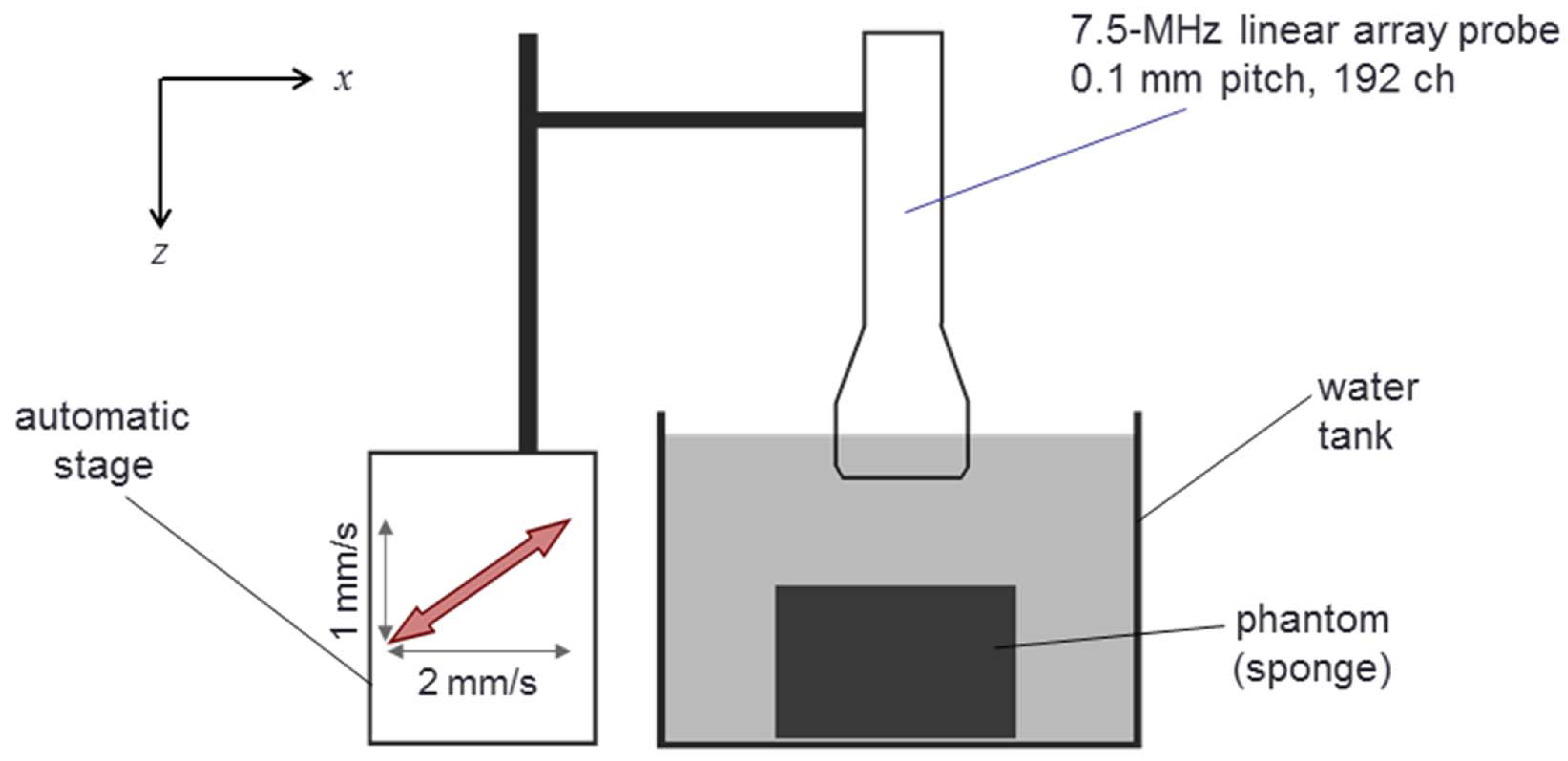
A linear array ultrasonic probe at a nominal center frequency of 7.5 MHz (PU-0558, Ueda Japan Radio, Ueda, Japan) was equipped to a custom-made ultrasound scanner (RSYS0002, Microsonic, Tokyo, Japan), which acquired ultrasonic echo signals from a sponge phantom received by individual transducer elements at a sampling frequency of 31.25 MHz, resulting in the axial sampling interval of 0.02464 mm (for both element and beamformed RF signals) by assuming the speed of sound as 1540 m/s. The element pitch of the linear array was 0.1 mm, which corresponds to the lateral sampling interval of the beamformed RF signals. As illustrated in Figure 1, the ultrasonic probe was moved by an automatic stage at constant lateral and axial velocities of 2 mm/s and -1 mm/s, respectively, which were the maximum velocities available by the automatic stage, to make the relative movement between the ultrasonic probe and the sponge phantom.
The transmit-receive sequence is described in [12]. In the present study, the number of emissions of plane waves for creation of one image frame was set at 4, and each plane wave was emitted using 96 transducer elements. In each transmission, 24 focused receiving beams were created at intervals of 0.1 mm, and the aperture used to create one focused receiving beam consisted of 72 elements. In the present study, the beamformed RF signals were obtained with rectangular apodization, Hanning apodization, and apodization consisting of two Hanning functions, which realized the lateral modulation of the ultrasonic field [31]. Consequently, one image frame consisting of 24 × 4 = 96 focused receiving beams was obtained by 4 emissions of plane waves. The frame rate achieved under such a transmit-receive condition was 1302 Hz at the pulse repetition frequency of 5208 Hz. The beamforming procedure was performed off-line on the ultrasound echo signals received by the individual elements using an in-house software. In the subsequent experimental validation, the point spread function obtained by the imaging method described above was evaluated by measuring an ultrasonic echo from a fine stainless wire of 15 m in diameter.
Owing to the high frame rate, as illustrated in Figure 2, temporal averaging was performed to obtain a set of velocity estimates for reduction of the variance in the estimates. To obtain cross spectra expressed by Equations (3)–(6) and (11), ultrasonic echoes in two frames, i.e., a frame set, are required. In the present study, as shown in Figure 2, the interval between two frames was set at 4, and the number of frame sets used for temporal averaging was also set at 4. If we assume that a typical target is the carotid arterial wall, its typical motion velocity is about 5 mm/s [37]. Under a condition of lateral and axial sampling intervals of 0.1 mm and 0.02464 mm, respectively, the frame rate required to avoid aliasing at the maximum frequency available in the frequency spectrum is . In the present study, the pulse repetition frequency was 5208 Hz, and a frame interval of 4 corresponded to a frame rate of 325.5 Hz, which was higher than 202.9 Hz.
In the subsequent experimental validation, the estimator defined by Equation (15) with the lateral and axial angular frequencies determined by Equations (16) and (17) was called as the conventional 2D motion estimator. The estimator defined by Equation (10) with the lateral and axial angular frequencies determined by Equations (20) and (21) was called as the proposed paired 1D motion estimators. The estimator defined by Equation (15) with the lateral and axial angular frequencies determined by Equations (20) and (21) was called as the proposed 2D motion estimator.
3. Experimental Results
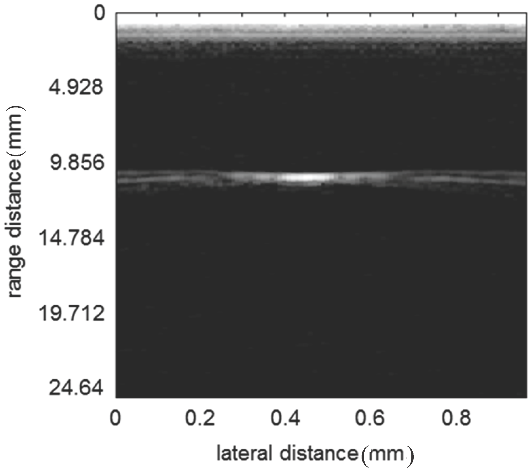
To evaluate the spatial resolution of the imaging method described in Section 2.4, an echo from a fine stainless wire of 15 m in diameter was measured in water. Figure 3 shows a B-mode image of the wire obtained with rectangular apodization. The lateral and axial widths at half maximum of the point spread function were 0.81 mm and 0.27 mm, respectively.
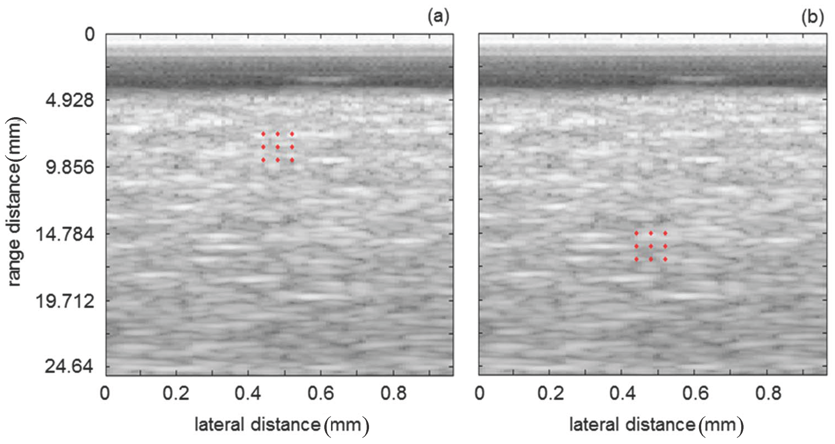
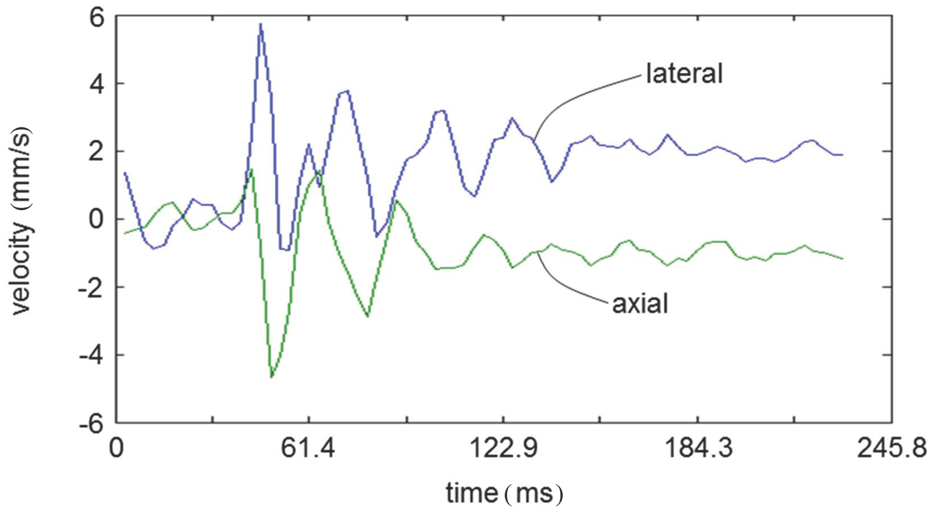
Figure 4a shows the B-mode image of the sponge phantom. The nine red points show the points of interest, at which the lateral and axial motion velocities are estimated. Examples of the estimated lateral and axial velocities are shown in Figure 5. As shown in Figure 5, at the beginning of the movement, there are undesirable vibrations of the metal arm, which supports the ultrasonic probe, due to the rapid acceleration of the automatic stage. Therefore, errors in the estimated lateral and axial velocities were evaluated during the period from 154 to 235 ms (25 frame sets) in Figure 5, when the undesired vibrations were attenuated. In the present paper, the bias error and standard deviation σ of the estimated lateral and axial velocities were evaluated as follows:
where is the lateral or axial velocity at p and n, which denote the points of interest () and the frame set number (), respectively, denotes averaging with respect to p and n, is the lateral or axial velocity averaged with respect to the points of interest and frame sets, and is the actual lateral or axial velocity, which was set to the automatic stage.
Table 1 and Table 2 show the bias errors and standard deviations σ of the lateral and axial velocities estimated by the conventional 2D motion estimator without and with frame averaging, respectively. The bias errors in the estimated lateral velocities were large when the lateral window size was less than ±1.5 mm (). On the other hand, the bias errors in the estimated axial velocities were very low (equal to or less than 3%) at all the examined window sizes. Both for the lateral and axial velocities, the standard deviations σ were significantly reduced by frame averaging.
Table 3 shows the bias errors and standard deviations σ of the lateral and axial velocities estimated by the proposed paired 1D motion estimators. Using the proposed paired 1D motion estimators, the bias errors of the estimated lateral velocities at small lateral window sizes of less than ±1.5 mm () were improved significantly compared with those of the conventional 2D motion estimator shown in Table 2, but the standard deviations σ were increased. The bias errors of the estimated axial velocities were very small (equal to or less than 2%) at all the examined window sizes.
Table 4 shows the bias errors and standard deviations σ of the lateral and axial velocities estimated by the proposed 2D motion estimator. At all the examined lateral window sizes, the bias errors of the estimated lateral velocities were improved dramatically compared with those of the conventional 2D motion estimator shown in Table 2. Also, the bias errors of the estimated axial velocities were very small (equal to or less than 2%) at all the examined window sizes.
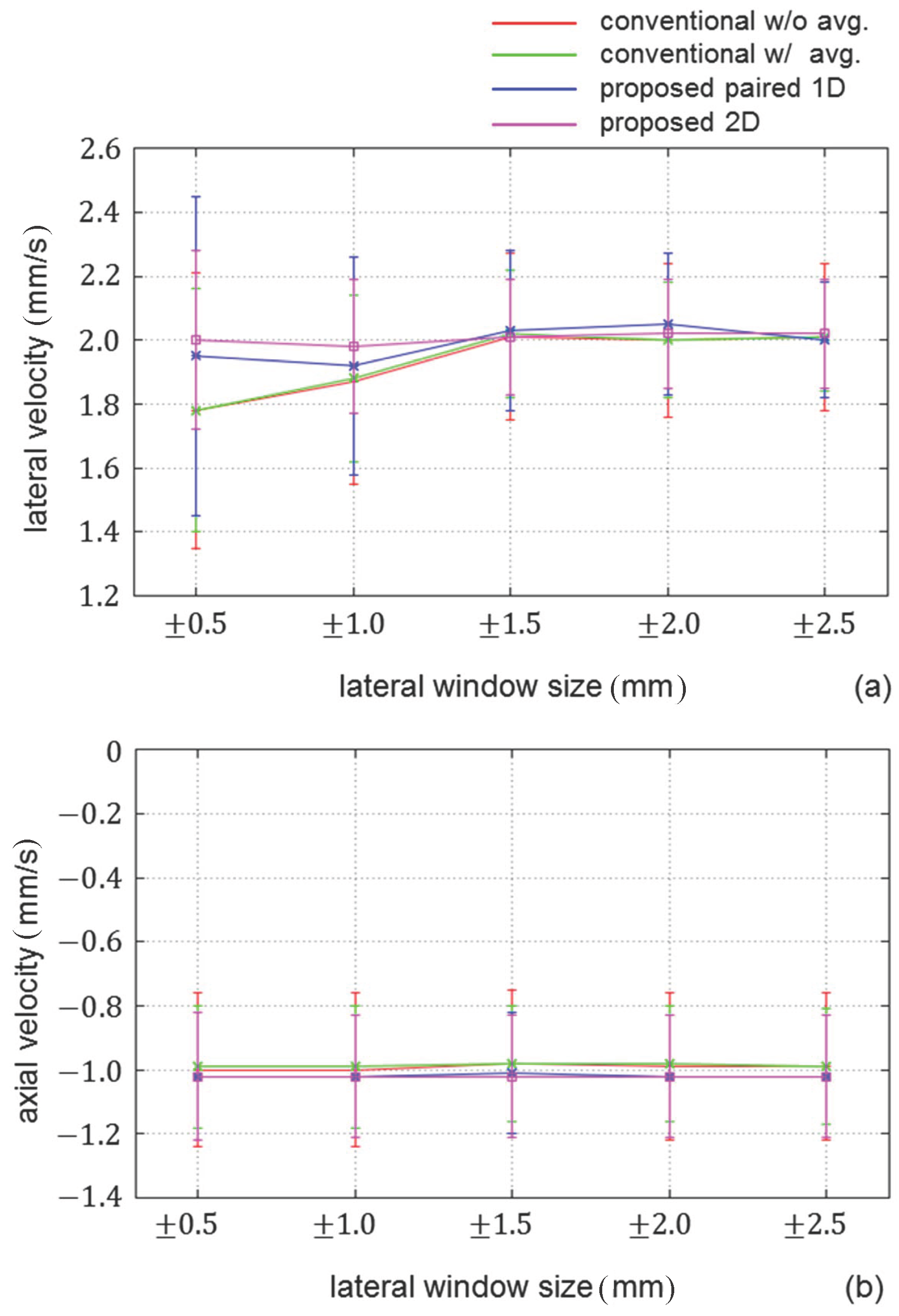
For a graphical representation of the results, means and standard deviations of the lateral and axial velocity estimates summarized in Table 1, Table 2, Table 3 and Table 4 are plotted in Figure 6a,b, respectively, as functions of the lateral window size. In Figure 6, the velocity estimates obtained with an axial window size of ±0.2464 mm are shown as a typical case because the velocity estimates are more dependent on the lateral window size. As can be seen in Figure 6a, the accuracy in estimation of the lateral velocity was improved significantly, particularly in cases of smaller lateral window sizes. On the other hand, the accuracy in estimation of the axial velocity was much less dependent on the window size.
To obtain the results shown in Table 1, Table 2, Table 3 and Table 4, rectangular apodization was used in receive beamforming to obtain the beamformed RF signals, which were analyzed by the conventional and proposed motion estimators to obtain the lateral and axial velocity estimates. Figure 7(1-b,2-b) show B-mode images of the phantom obtained with Hanning apodization and apodization consisting of two Hanning functions (lateral modulation), respectively.
Table 5 shows the errors and standard deviations σ of the lateral and axial velocities estimated by analyzing the RF signals beamformed with Hanning apodization using the proposed 2D motion estimator. Although the bias errors and standard deviations σ of the estimated axial velocities are very similar to those obtained with rectangular apodization shown in Table 4, the bias errors and standard deviations σ of the lateral velocity estimates are degraded. The lateral velocity estimates obtained with lateral modulation (Table 6) are much better than those obtained with Hanning apodization (Table 5), but the lateral velocity estimates obtained with rectangular apodization (Table 4) are significantly better than those obtained with lateral modulation when the lateral window size is smaller than ±1.5 mm ().
In ultrasonic imaging, the point spread function varies with depth, i.e., the spatial resolution in a deep region is worse than that in a shallow region. To examine the effect of the change in the point spread function on the accuracies of the estimators, errors in the displacements estimated at nine red points shown in Figure 4b were also evaluated. Table 7 and Table 8 show the bias errors and standard deviations σ of the lateral and axial velocity estimates obtained by the conventional and proposed 2D motion estimators, respectively, with rectangular apodization. The lateral velocity estimates obtained by the conventional 2D motion estimator were much more affected by degradation of the spatial resolution than those obtained by the proposed 2D motion estimator. For both methods, the axial velocity estimates were less dependent on depth.
Furthermore, the proposed method was evaluated with a different motion velocity of the automatic stage, i.e., lateral and axial velocities of 1 mm/s and 0.5 mm/s, respectively. Table 9 and Table 10 show the lateral and axial velocities estimated at the same points shown in Figure 4a obtained by the conventional and proposed 2D motion estimators, respectively. As in the results with higher lateral and axial velocities shown in Table 2 and Table 4, respectively, bias errors in the lateral velocity estimates were significantly reduced by the proposed method at a small lateral window size of mm.
4. Discussion
In the present study, two phase-sensitive motion estimators, namely, the proposed paired 1D motion estimators and the proposed 2D motion estimator, were developed and examined by the phantom experiment. Both proposed methods significantly reduced the bias errors in the lateral velocity estimates compared with the conventional 2D motion estimator particularly when the lateral window size was small. However, the performance of the proposed paired 1D motion estimators was worse than the proposed 2D motion estimator. The reason for this can be considered as follows: To estimate the displacement in the direction of interest (lateral or axial direction), Salles et al. remove the phase shift of the ultrasonic echo caused by the displacement in the other direction from the total phase shift using the narrow band analytical signal obtained by the Hilbert transform [35]. In the proposed paired 1D motion estimators, similar procedures were done by Equation (7) by assuming that the absolute values of the mean frequencies of the components and were same, i.e., . However, the absolute values of the mean frequencies of the components and were not always same due to the ambiguity in the mean frequency of each component of the spectrum, particularly when the window size was small, as described in Section 2.3. As a result, the velocity estimate in the direction of interest was degraded because the phase shift caused by the displacement in the other direction was not removed accurately from the total phase shift. The proposed 2D motion estimator realized the best performance among the three methods examined in the present study because it did not assume that the absolute values of the mean frequencies of the components and were same and estimates the mean frequency of each component of spectrum.
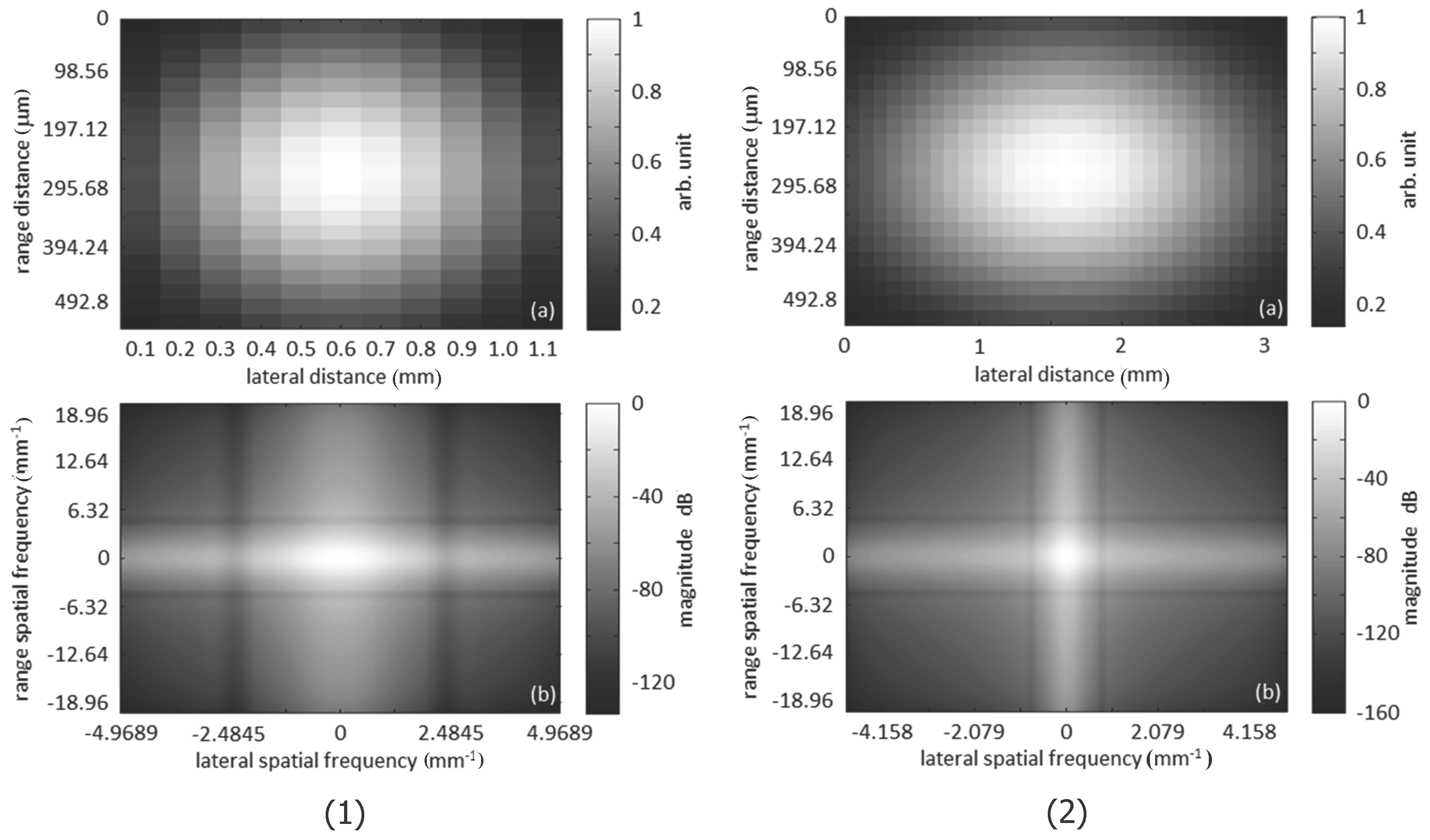
As shown by the results in Table 2, the conventional 2D motion estimator requires a window size, which is larger than or equal to ±1.5 mm () in the lateral direction and ±0.2464 mm () in the axial direction, to reduce the bias error in the lateral velocity estimates. The Gaussian spatial windows used in the discrete Fourier transform and their frequency spectra are shown in Figure 8. Figure 8(1-a) shows the Gaussian window with the lateral and axial sizes of (±0.5 mm (), ±0.2464 mm ()), respectively, and Figure 8(1-b) shows its power spectrum. Figure 8(2-a,2-b) show those of the Gaussian window with the lateral and axial sizes of (±1.5 mm (), ±0.2464 mm ()), respectively. The lateral widths at half maximum of the main lobe of the power spectra shown in Figure 8(1-b,2-b) are 1.24 mm and 0.42 m, respectively. Therefore, the results obtained in the present study showed that the main lobe width of less than or equal to 0.42 mm was required to obtain accurate lateral velocity estimates by the conventional 2D motion estimator. The main lobe width was compared with the size of the point spread function of the beamformed ultrasonic data. The lateral width at half maximum of 0.42 m corresponds to about three times of the lateral width at half maximum of the point spread function shown in Figure 3 [].
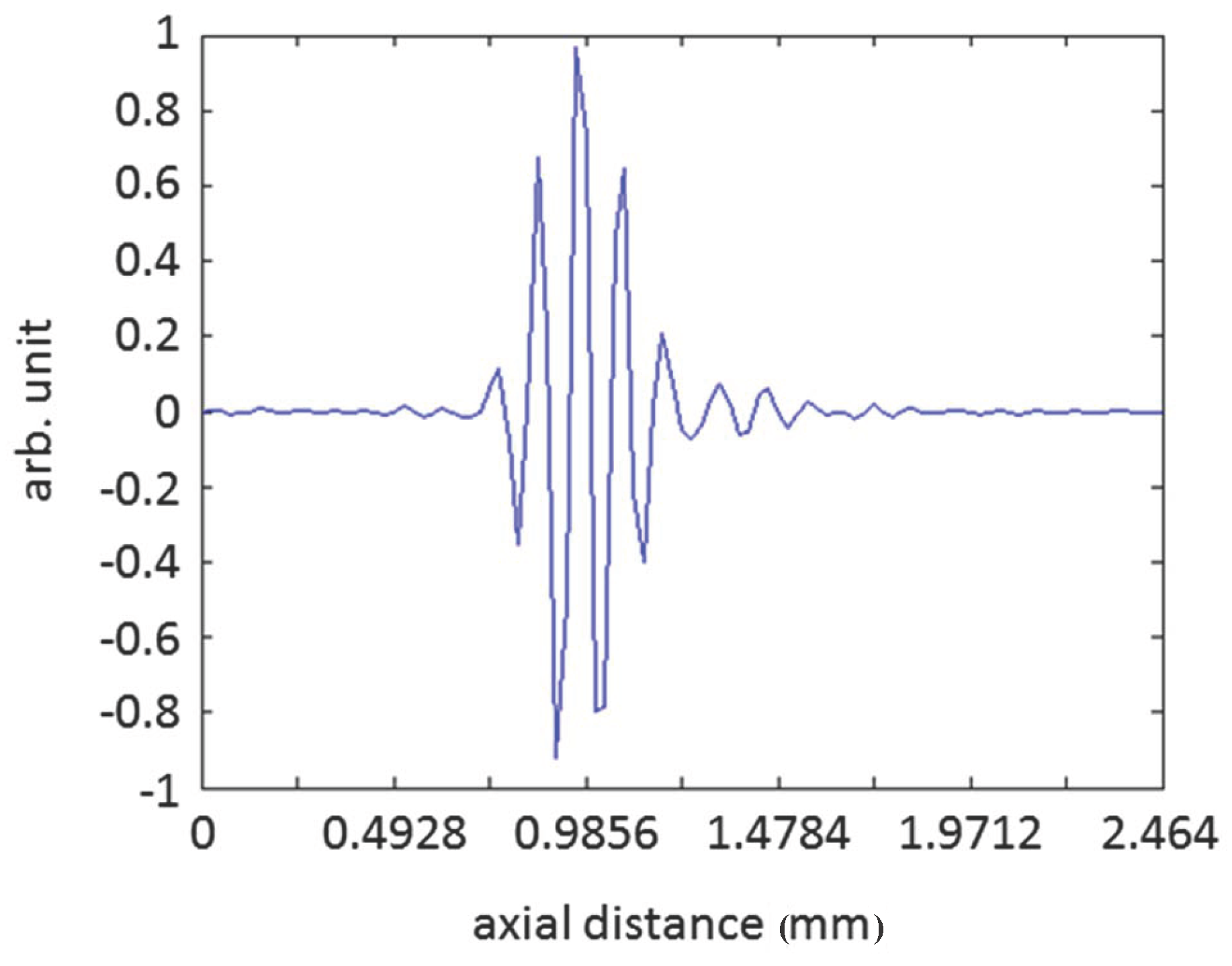
On the other hand, the accurate axial velocity estimates could be obtained even with a smaller axial window size of ±0.1232 mm, which almost corresponds to the axial size of the point spread function. Figure 9 shows the beamformed RF signal obtained along the scan line, which pass through the peak of the point spread function shown in Figure 3. As can be seen in Figure 9, in the axial direction, there are about three cycles of the ultrasonic signal in the axial width at half maximum of 0.27 mm of the point spread function, which almost corresponds to an axial window size of ±0.1232 mm. In the lateral direction, it can be considered that there is only one cycle of signal variation within the point spread function. Therefore, a window size of three times of the point spread function was required in the lateral direction to include three cycles of the ultrasonic signal variation. From these results, it was supposed that the conventional 2D motion estimator gives accurate velocity estimate when the spatial window includes about three cycles of the ultrasonic signal variation in both lateral and axial direction.
As described above, the conventional 2D motion estimator requires a relatively large spatial window to obtain accurate lateral and axial motion estimates. On the other hand, the proposed 2D motion estimator realizes accurate estimation of the lateral and axial motion with a smaller spatial window. Such a property of the proposed 2D motion estimator is preferable for more regional measurement of the tissue motion by means of ultrasound.
In this study, the basic concept of the proposed 2D motion estimator was presented, and the proposed method was implemented with a linear array probe. Also, the feasibility of the proposed method for 2D motion detection was shown by a primitive phantom experiment. In future work, an experimental validation using a more realistic phantom should be performed and, also, the proposed motion estimator should be implemented with phased and curved arrays.
5. Conclusions
Accurate motion estimators play a key role in measurement of tissue dynamics. In high-frame-rate ultrasound, the tissue displacement between frames is small owing to the high temporal resolution and, thus, a phase-sensitive motion estimator is feasible because a small displacement does not cause the aliasing effect. In the present study, 2D motion estimators were examined by the basic experiment using a phantom. The results showed that the proposed 2D motion estimator using shifted cross spectra achieved significantly better lateral and axial velocity estimates than the conventional 2D motion estimator by reducing the ambiguity in the frequency of each component of the cross spectrum. The proposed 2D motion estimator gave accurate velocity estimates even with a smaller spatial window than the conventional 2D motion estimator, which is one of the big advantages of the proposed method for more regional measurement of the tissue motion.
Acknowledgments
This study was supported by JSPS KAKENHI Grant Numbers 26289123 and 15K13995.
Conflicts of Interest
The author declares no conflict of interest.
References
- Ophir, J.; Céspedes, I.; Ponnekanti, H.; Yazdi, Y.; Li, X. Elastography: A quantitative method for imaging the elasticity of biological tissues. Ultrason. Imaging 1991, 13, 111–134. [Google Scholar] [CrossRef] [PubMed]
- Hasegawa, H.; Kanai, H.; Chubachi, N.; Koiwa, Y. Noninvasive evaluation of Poisson’s ratio of arterial wall using ultrasound. Electronics Lett. 1997, 33, 340–342. [Google Scholar] [CrossRef]
- De Korte, C.L.; van der Steen, A.F.; Céspedes, E.I.; Pasterkamp, G. Intravascular ultrasound elastography in human arteries: Initial experience in vitro. Ultrasound Med. Biol. 1998, 24, 401–408. [Google Scholar] [CrossRef]
- Kanai, H.; Hasegawa, H.; Koiwa, Y.; Ichiki, M.; Tezuka, F. Elasticity imaging of atheroma with transcutaneous ultrasound -Preliminary study-. Circulation 2003, 107, 3018–3021. [Google Scholar] [CrossRef] [PubMed]
- Maurice, R.L.; Soulez, G.; Giroux, M.D.; Cloutier, G. Noninvasive vascular elastography for carotid artery characterization on subjects without previous history of atherosclerosis. Med. Phys. 2008, 35, 3436–3443. [Google Scholar] [CrossRef] [PubMed]
- Kanai, H.; Hasegawa, H.; Chubachi, N.; Koiwa, Y.; Tanaka, M. Noninvasive evaluation of local myocardial thickening and its color-coded imaging. IEEE Trans. Ultrason. Ferroelectr. Freq. Control 1997, 44, 752–768. [Google Scholar] [CrossRef]
- Heimdal, A.; Støylen, A.; Torp, H.; Skjærpe, T. Real time strain rate imaging of the left ventricle by ultrasound. J. Am. Soc. Echocardiogr. 1998, 11, 1013–1019. [Google Scholar] [CrossRef]
- D’hooge, J.; Heimdal, A.; Jamal, F.; Kukulski, T.; Bijnens, B.; Rademakers, F.; Hatle, L.; Suetens, P.; Sutherland, G.R. Regional strain and strain rate measurements by cardiac ultrasound: Principles, implementation and limitations. Eur. J. Echocardiogr. 2000, 1, 154–170. [Google Scholar] [CrossRef] [PubMed]
- Smiseth, O.A.; Torp, H.; Opdahl, A.; Haugaa, H.; Urheim, S. Myocardial strain imaging: How useful is it in clinical decision making? Eur. Heart J. 2015, in press. [Google Scholar] [CrossRef] [PubMed]
- Shattuck, D.P.; Weinshenker, M.D.; Smith, S.W.; von Ramm, O.T. Explososcan: A parallel processing technique for high speed ultrasound imaging with linear phased arrays. J. Acoust. Soc. Amer. 1984, 75, 1273–1282. [Google Scholar] [CrossRef]
- Tanter, M.; Bercoff, J.; Sandrin, L.; Fink, M. Ultrafast compound imaging for 2-D motion vector estimation: Application to transient elastography. IEEE Trans. Ultrason. Ferroelectr. Freq. Control 2002, 49, 1363–1374. [Google Scholar] [CrossRef] [PubMed]
- Hasegawa, H.; Kanai, H. Simultaneous imaging of artery-wall strain and blood flow by high frame rate acquisition of RF signals. IEEE Trans. Ultrason. Ferroelectr. Freq. Control 2008, 55, 2626–2639. [Google Scholar] [CrossRef] [PubMed]
- Bercoff, J.; Montaldo, G.; Loupas, T.; Savery, D.; Mézière, F.; Fink, M.; Tanter, M. Ultrafast compound Doppler imaging: Providing full blood flow characterization. IEEE Trans. Ultrason. Ferroelectr. Freq. Control 2011, 58, 134–147. [Google Scholar] [CrossRef] [PubMed]
- Yiu, B.Y.; Yu, A.C. High-frame-rate ultrasound color-encoded speckle imaging of complex flow dynamics. Ultrasound Med. Biol. 2013, 39, 1015–1025. [Google Scholar] [CrossRef] [PubMed]
- Hasegawa, H.; Hongo, K.; Kanai, H. Measurement of regional pulse wave velocity using very high frame rate ultrasound. J. Med. Ultrason. 2013, 40, 91–98. [Google Scholar] [CrossRef] [PubMed]
- Nagaoka, R.; Iwasaki, R.; Arakawa, M.; Kobayashi, K.; Yoshizawa, S.; Umemura, S.; Saijo, Y. Basic study of intrinsic elastography: Relationship between tissue stiffness and propagation velocity of deformation induced by pulsatile flow. Jpn. J. Appl. Phys. 2015, 54. [Google Scholar] [CrossRef]
- Honjo, Y.; Hasegawa, H.; Kanai, H. Two-dimensional tracking of heart wall for detailed analysis of heart function at high temporal and spatial resolutions. Jpn. J. Appl. Phys. 2010, 49. [Google Scholar] [CrossRef]
- Provost, J.; Gambhir, A.; Vest, J.; Garan, H.; Konofagou, E.E. A clinical feasibility study of atrial and ventricular electromechanical wave imaging. Heart Rhythm 2013, 10, 856–862. [Google Scholar] [CrossRef] [PubMed]
- Shahmirzadi, D.; Li, R.X.; Konofagou, E.E. Pulse-wave propagation in straight-geometry vessels for stiffness estimation: Theory, simulations, phantoms and in vitro findings. J. Biomechan. Eng. 2012, 134, 114502-1–114502-6. [Google Scholar] [CrossRef] [PubMed]
- Takahashi, H.; Hasegawa, H.; Kanai, H. Echo speckle imaging of blood particles with high-frame-rate echocardiography. Jpn. J. Appl. Phys. 2014, 53. [Google Scholar] [CrossRef]
- Takahashi, H.; Hasegawa, H.; Kanai, H. Temporal averaging of two-dimensional correlation functions for velocity vector imaging of cardiac blood flow. J. Med. Ultrason. 2015, 42, 323–330. [Google Scholar] [CrossRef] [PubMed]
- Montaldo, G.; Tanter, M.; Bercoff, J.; Benech, N.; Fink, M. Coherent plane-wave compounding for very high-frame rate ultrasonography and transient elastography. IEEE Trans. Ultrason. Ferroelectr. Freq. Control 2009, 56, 489–506. [Google Scholar] [CrossRef] [PubMed]
- Tong, L.; Gao, H.; D’hooge, J. Multi-transmit beam forming for fast cardiac imaging—a simulation study. IEEE Trans. Ultrason. Ferroelectr. Freq. Control 2013, 60, 1719–1731. [Google Scholar] [CrossRef] [PubMed]
- Hasegawa, H.; Kanai, H. Effect of sub-aperture beamforming on phase coherence imaging. IEEE Trans. Ultrason. Ferroelectr. Freq. Control 2014, 61, 1779–1790. [Google Scholar] [CrossRef] [PubMed]
- Hasegawa, H.; Kanai, H. Effect of element directivity on adaptive beamforming applied to high-frame-rate ultrasound. IEEE Trans. Ultrason. Ferroelectr. Freq. Control 2015, 62, 511–523. [Google Scholar] [CrossRef] [PubMed]
- Hasegawa, H. Enhancing effect of phase coherence factor for improvement of spatial resolution in ultrasonic imaging. J. Med. Ultrason. 2016, 43, 19–27. [Google Scholar] [CrossRef] [PubMed]
- Kasai, C.; Namekawa, K.; Koyano, A.; Omoto, R. Real-time two-dimensional blood flow imaging using an autocorrelation technique. IEEE Trans. Sonics Ultrason. 1985, SU-32, 458–464. [Google Scholar] [CrossRef]
- Céspedes, I.; Huang, Y.; Ophir, J.; Spratt, S. Methods for estimation of subsample time delays of digitized echo signals. Ultrason. Imaging 1995, 17, 142–171. [Google Scholar] [CrossRef] [PubMed]
- Loupas, T.; Powers, J.T.; Gill, R.W. An axial velocity estimator for ultrasound blood flow imaging, based on a full evaluation of the Doppler equation by means of a two-dimensional autocorrelation approach. IEEE Trans. Ultrason. Ferroelectr. Freq. Control 1995, 42, 672–688. [Google Scholar] [CrossRef]
- Sumi, C.; Suzuki, A.; Nakayama, K. Phantom experiment on estimation of shear modulus distribution in soft tissue from ultrasonic measurement of displacement vector field. IEICE Trans. Fundam. 1995, E78-A, 1655–1664. [Google Scholar]
- Jensen, J.A. A new method for estimation of velocity vectors. IEEE Trans. Ultrason. Ferroelectr. Freq. Control 1998, 45, 837–851. [Google Scholar] [CrossRef] [PubMed]
- Chen, X.; Zohdy, M.J.; Emelianov, S.Y.; O’Donnell, M. Lateral speckle tracking using synthetic lateral phase. IEEE Trans. Ultrason. Ferroelectr. Freq. Control 2004, 51, 540–550. [Google Scholar] [CrossRef] [PubMed]
- Sumi, C. Displacement vector measurement using instantaneous ultrasound signal phase–Multidimensional autocorrelation and Doppler methods. IEEE Trans. Ultrason. Ferroelectr. Freq. Control 2008, 55, 24–43. [Google Scholar] [CrossRef] [PubMed]
- Hasegawa, H.; Kanai, H. Phase-sensitive lateral motion estimator for measurement of artery-wall displacement –Phantom study. IEEE Trans. Ultrason. Ferroelectr. Freq. Control 2009, 56, 2450–2462. [Google Scholar] [CrossRef] [PubMed]
- Salles, S.; Chee, A.J.Y.; Garcia, D.; Yu, A.C.H.; Vray, D.; Liebgott, H. 2-D arterial wall motion imaging using ultrafast ultrasound and transverse oscillations. IEEE Trans. Ultrason. Ferroelectr. Freq. Control 2015, 62, 1047–1058. [Google Scholar] [CrossRef] [PubMed]
- Kawanaka, A.; Nakayama, K. A method of polarity estimation for reflected echo in ultrasonotomography. IEICE Trans. 1980, J63-A, 437–443. (In Japanese) [Google Scholar]
- Hasegawa, H.; Sato, M.; Irie, T. High resolution wavenumber analysis for investigation of arterial pulse wave propagation. Jpn. J. Appl. Phys. 2016, 55. [Google Scholar] [CrossRef]
Figure 1.
Ilustration of experimental setup.

Figure 2.
Illustration of frame averaging procedure in velocity estimation.
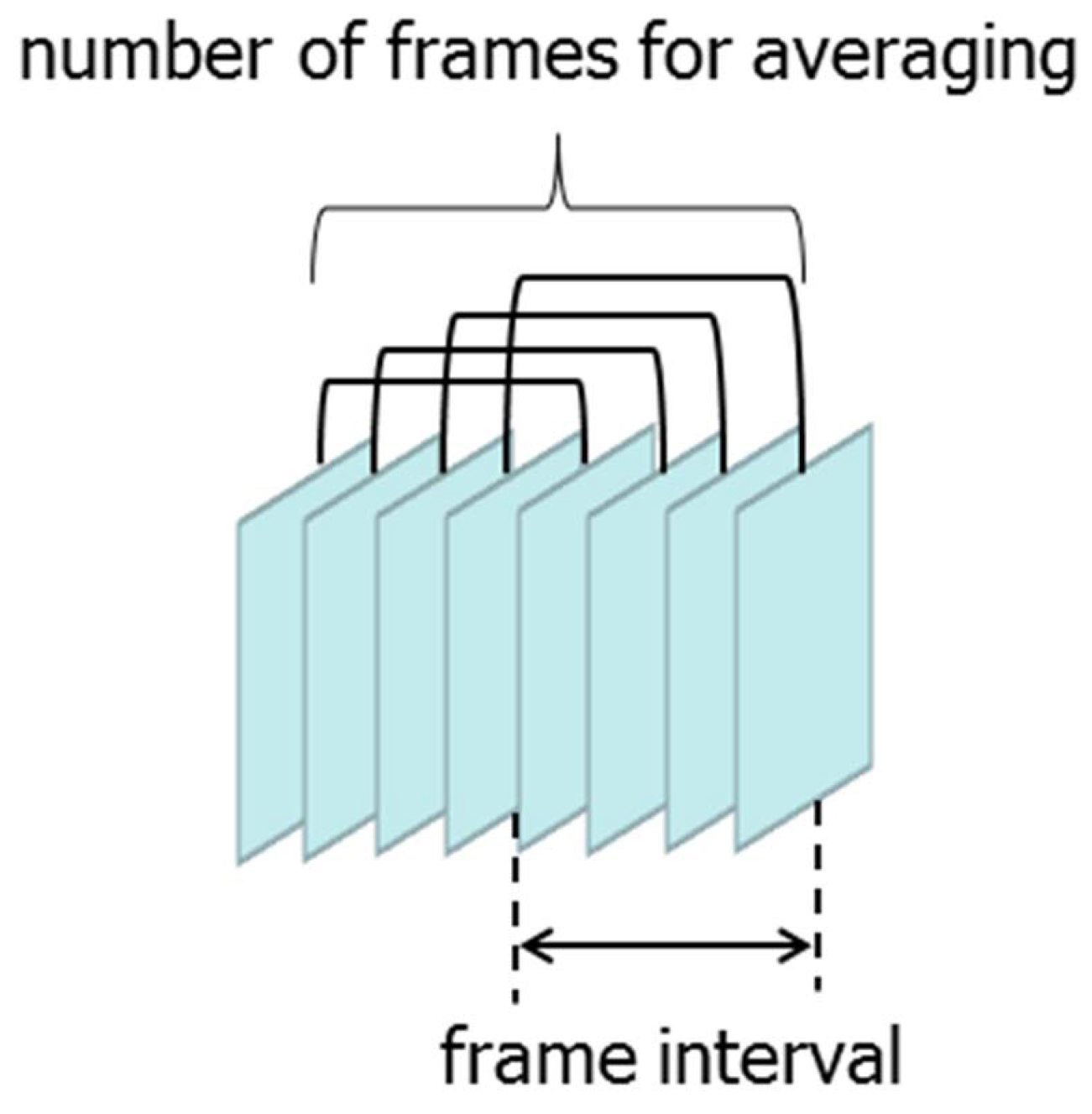
Figure 3.
B-mode image of a stainless wire at 15 m in diameter.

Figure 4.
B-mode image of phantom. Red points are points in shallow (a) and deep (b) regions of interest to be tracked.
Figure 4.
B-mode image of phantom. Red points are points in shallow (a) and deep (b) regions of interest to be tracked.

Figure 5.
Example of estimated lateral and axial motion velocities. Lateral and axial velocities set at the automatic stage were 2.0 mm/s and –1.0 mm/s, respectively.
Figure 5.
Example of estimated lateral and axial motion velocities. Lateral and axial velocities set at the automatic stage were 2.0 mm/s and –1.0 mm/s, respectively.

Figure 6.
Lateral (a) and axial (b) velocity estimates obtained by respective methods.

Figure 7.
B-mode images of phantom obtained with (1) Hanning apodization and (2) lateral modulation [31]. (a) Receive apodization. (b) B-mode image.
Figure 7.
B-mode images of phantom obtained with (1) Hanning apodization and (2) lateral modulation [31]. (a) Receive apodization. (b) B-mode image.
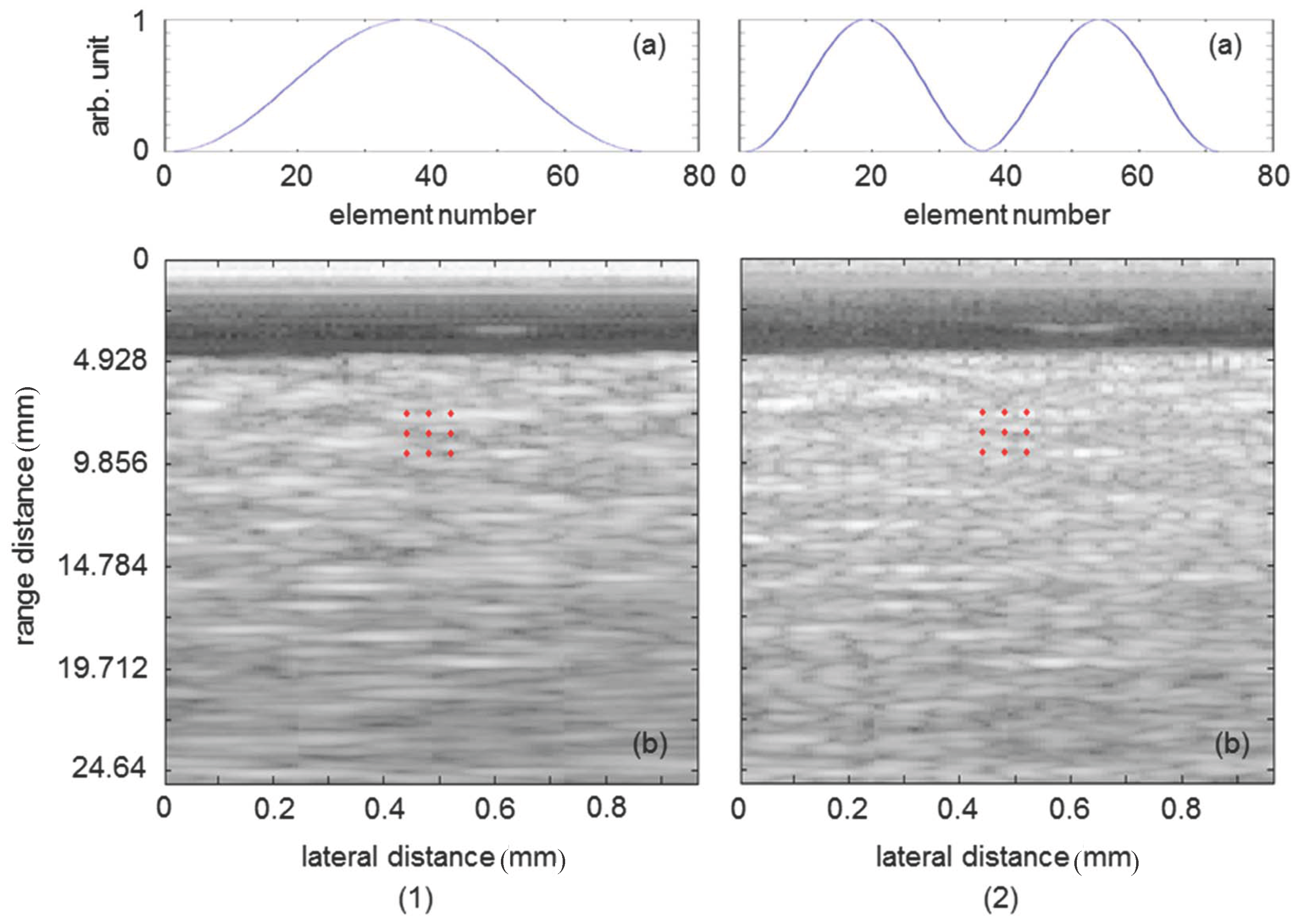
Figure 8.
2D Gaussian spatial windows used for discrete Fourier transform (a) and their power spectra (b). Lateral and axial window sizes are (±0.5 mm (), ±0.2464 mm ()) (1) and (±1.5 mm (), ±0.2464 mm ()) (2).
Figure 8.
2D Gaussian spatial windows used for discrete Fourier transform (a) and their power spectra (b). Lateral and axial window sizes are (±0.5 mm (), ±0.2464 mm ()) (1) and (±1.5 mm (), ±0.2464 mm ()) (2).

Figure 9.
Beamformed radio-frequency (RF) signal obtained along a scan line, which passes through the peak of the point spread function shown in Figure 3.
Figure 9.
Beamformed radio-frequency (RF) signal obtained along a scan line, which passes through the peak of the point spread function shown in Figure 3.

Table 1.
Bias errors and standard deviations σ of lateral and axial displacements at nine red points in Figure 4a estimated by the conventional 2D motion estimator without frame averaging. Beamformed echo signals were obtained with rectangular apodization. Actual lateral and axial velocities were 2 mm/s and –1 mm/s, respectively.
| Bias Errors and Standard Deviation of Estimated Lateral Velocities (mm/s) | |||||
| axial window size (mm) (K) | lateral window size (mm) (M) | ||||
| ±0.5 (5) | ±1.0 (10) | ±1.5 (15) | ±2.0 (20) | ±2.5 (25) | |
| ±0.1232 (5) | |||||
| ±0.2464 (10) | |||||
| ±0.3696 (15) | |||||
| ±0.4928 (20) | |||||
| Bias Errors and Standard Deviation of Estimated Axial Velocities (mm/s) | |||||
| axial window size (mm) (K) | lateral window size (mm) (M) | ||||
| ±0.5 (5) | ±1.0 (10) | ±1.5 (15) | ±2.0 (20) | ±2.5 (25) | |
| ±0.1232 (5) | |||||
| ±0.2464 (10) | |||||
| ±0.3696 (15) | |||||
| ±0.4928 (20) | |||||
Table 2.
Bias errors and standard deviations σ of lateral and axial displacements at nine red points in Figure 4a estimated by the conventional 2D motion estimator with frame averaging. Beamformed echo signals were obtained with rectangular apodization. Actual lateral and axial velocities were 2 mm/s and –1 mm/s, respectively.
| Bias Errors and Standard Deviation of Estimated Lateral Velocities (mm/s) | |||||
| axial window size (mm) (K) | lateral window size (mm) (M) | ||||
| ±0.5 (5) | ±1.0 (10) | ±1.5 (15) | ±2.0 (20) | ±2.5 (25) | |
| ±0.1232 (5) | |||||
| ±0.2464 (10) | |||||
| ±0.3696 (15) | |||||
| ±0.4928 (20) | |||||
| Bias Errors and Standard Deviation of Estimated Axial Velocities (mm/s) | |||||
| axial window size (mm) (K) | lateral window size (mm) (M) | ||||
| ±0.5 (5) | ±1.0 (10) | ±1.5 (15) | ±2.0 (20) | ±2.5 (25) | |
| ±0.1232 (5) | |||||
| ±0.2464 (10) | |||||
| ±0.3696 (15) | |||||
| ±0.4928 (20) | |||||
Table 3.
Bias errors and standard deviations σ of lateral and axial displacements at nine red points in Figure 4a estimated by the proposed paired 1D motion estimators with frame averaging. Beamformed echo signals were obtained with rectangular apodization. Actual lateral and axial velocities were 2 mm/s and –1 mm/s, respectively.
| Bias Errors and Standard Deviation of Estimated Lateral Velocities (mm/s) | |||||
| axial window size (mm) (K) | lateral window size (mm) (M) | ||||
| ±0.5 (5) | ±1.0 (10) | ±1.5 (15) | ±2.0 (20) | ±2.5 (25) | |
| ±0.1232 (5) | |||||
| ±0.2464 (10) | |||||
| ±0.3696 (15) | |||||
| ±0.4928 (20) | |||||
| Bias Errors and Standard Deviation of Estimated Axial Velocities (mm/s) | |||||
| axial window size (mm) (K) | lateral window size (mm) (M) | ||||
| ±0.5 (5) | ±1.0 (10) | ±1.5 (15) | ±2.0 (20) | ±2.5 (25) | |
| ±0.1232 (5) | |||||
| ±0.2464 (10) | |||||
| ±0.3696 (15) | |||||
| ±0.4928 (20) | |||||
Table 4.
Bias errors and standard deviations σ of lateral and axial displacements at nine red points in Figure 4a estimated by the proposed 2D motion estimator with frame averaging. Beamformed echo signals were obtained with rectangular apodization. Actual lateral and axial velocities were 2 mm/s and –1 mm/s, respectively.
| Bias Errors and Standard Deviation of Estimated Lateral Velocities (mm/s) | |||||
| axial window size (mm) (K) | lateral window size (mm) (M) | ||||
| ±0.5 (5) | ±1.0 (10) | ±1.5 (15) | ±2.0 (20) | ±2.5 (25) | |
| ±0.1232 (5) | |||||
| ±0.2464 (10) | |||||
| ±0.3696 (15) | |||||
| ±0.4928 (20) | |||||
| Bias Errors and Standard Deviation of Estimated Axial Velocities (mm/s) | |||||
| axial window size (mm) (K) | lateral window size (mm) (M) | ||||
| ±0.5 (5) | ±1.0 (10) | ±1.5 (15) | ±2.0 (20) | ±2.5 (25) | |
| ±0.1232 (5) | |||||
| ±0.2464 (10) | |||||
| ±0.3696 (15) | |||||
| ±0.4928 (20) | |||||
Table 5.
Bias errors and standard deviations σ of lateral and axial displacements at nine red points in Figure 4a estimated by the proposed 2D motion estimator with frame averaging. Beamformed echo signals were obtained with Hanning apodization. Actual lateral and axial velocities were 2 mm/s and –1 mm/s, respectively.
| Bias Errors and Standard Deviation of Estimated Lateral Velocities (mm/s) | |||||
| axial window size (mm) (K) | lateral window size (mm) (M) | ||||
| ±0.5 (5) | ±1.0 (10) | ±1.5 (15) | ±2.0 (20) | ±2.5 (25) | |
| ±0.1232 (5) | |||||
| ±0.2464 (10) | |||||
| ±0.3696 (15) | |||||
| ±0.4928 (20) | |||||
| Bias Errors and Standard Deviation of Estimated Axial Velocities (mm/s) | |||||
| axial window size (mm) (K) | lateral window size (mm) (M) | ||||
| ±0.5 (5) | ±1.0 (10) | ±1.5 (15) | ±2.0 (20) | ±2.5 (25) | |
| ±0.1232 (5) | |||||
| ±0.2464 (10) | |||||
| ±0.3696 (15) | |||||
| ±0.4928 (20) | |||||
Table 6.
Bias errors and standard deviations σ of lateral and axial displacementsat nine red points in Figure 4a estimated by the proposed 2D motion estimator with frame averaging. Beamformed echo signals were obtained with apodization of two Hanning functions (lateral modulation) [31]. Actual lateral and axial velocities were 2 mm/s and –1 mm/s, respectively.
| Bias Errors and Standard Deviation of Estimated Lateral Velocities (mm/s) | |||||
| axial window size (mm) (K) | lateral window size (mm) (M) | ||||
| ±0.5 (5) | ±1.0 (10) | ±1.5 (15) | ±2.0 (20) | ±2.5 (25) | |
| ±0.1232 (5) | |||||
| ±0.2464 (10) | |||||
| ±0.3696 (15) | |||||
| ±0.4928 (20) | |||||
| Bias Errors and Standard Deviation of Estimated Axial Velocities (mm/s) | |||||
| axial window size (mm) (K) | lateral window size (mm) (M) | ||||
| ±0.5 (5) | ±1.0 (10) | ±1.5 (15) | ±2.0 (20) | ±2.5 (25) | |
| ±0.1232 (5) | |||||
| ±0.2464 (10) | |||||
| ±0.3696 (15) | |||||
| ±0.4928 (20) | |||||
Table 7.
Bias errors and standard deviations σ of lateral and axial displacements at nine red points in Figure 4b estimated by the conventional 2D motion estimator with frame averaging. Beamformed echo signals were obtained with rectangular apodization. Actual lateral and axial velocities were 2 mm/s and –1 mm/s, respectively.
| Bias Errors and Standard Deviation of Estimated Lateral Velocities (mm/s) | |||||
| axial window size (mm) (K) | lateral window size (mm) (M) | ||||
| ±0.5 (5) | ±1.0 (10) | ±1.5 (15) | ±2.0 (20) | ±2.5 (25) | |
| ±0.1232 (5) | –0.76 ± 0.50 | –0.30 ± 0.80 | –0.10 ± 0.98 | –0.27 ± 0.63 | –0.33 ± 0.61 |
| ±0.2464 (10) | –0.77 ± 0.42 | –0.36 ± 0.48 | –0.25 ± 0.47 | –0.20 ± 0.38 | –0.16 ± 0.32 |
| ±0.3696 (15) | –0.65 ± 0.43 | -0.20 ± 0.38 | –0.15 ± 0.39 | –0.11 ± 0.38 | –0.08 ± 0.31 |
| ±0.4928 (20) | –0.67 ± 0.39 | –0.19 ± 0.32 | –0.06 ± 0.32 | –0.05 ± 0.30 | –0.06 ± 0.27 |
| Bias Errors and Standard Deviation of Estimated Axial Velocities (mm/s) | |||||
| axial window size (mm) (K) | lateral window size (mm) (M) | ||||
| ±0.5 (5) | ±1.0 (10) | ±1.5 (15) | ±2.0 (20) | ±2.5 (25) | |
| ±0.1232 (5) | 0.02 ± 0.18 | 0.03 ± 0.18 | 0.05 ± 0.17 | 0.05 ± 0.17 | 0.05 ± 0.18 |
| ±0.2464 (10) | 0.00 ± 0.19 | 0.01 ± 0.19 | 0.02 ± 0.19 | 0.01 ± 0.19 | 0.01 ± 0.19 |
| ±0.3696 (15) | 0.00 ± 0.19 | 0.00 ± 0.18 | 0.01 ± 0.18 | 0.01 ± 0.18 | 0.01 ± 0.18 |
| ±0.4928 (20) | 0.00 ± 0.19 | 0.00 ± 0.19 | 0.01 ± 0.18 | 0.01 ± 0.18 | 0.01 ± 0.18 |
Table 8.
Bias errors and standard deviations σ of lateral and axial displacements at nine red points in Figure 4b estimated by the proposed 2D motion estimator with frame averaging. Beamformed echo signals were obtained with rectangular apodization. Actual lateral and axial velocities were 2 mm/s and –1 mm/s, respectively.
| Bias Errors and Standard Deviation of Estimated Lateral Velocities (mm/s) | |||||
| axial window size (mm) (K) | lateral window size (mm) (M) | ||||
| ±0.5 (5) | ±1.0 (10) | ±1.5 (15) | ±2.0 (20) | ±2.5 (25) | |
| ±0.1232 (5) | 0.11 ± 0.71 | 0.06 ± 0.57 | 0.03 ± 0.56 | 0.07 ± 0.41 | –0.04 ± 0.37 |
| ±0.2464 (10) | –0.06 ± 0.51 | 0.01 ± 0.45 | –0.02 ± 0.42 | 0.03 ± 0.36 | 0.01 ± 0.33 |
| ±0.3696 (15) | 0.01 ± 0.47 | 0.07 ± 0.42 | –0.01 ± 0.39 | -0.01 ± 0.35 | –0.02 ± 0.32 |
| ±0.4928 (20) | 0.03 ± 0.44 | 0.06 ± 0.39 | 0.05 ± 0.35 | 0.05 ± 0.31 | 0.01 ± 0.28 |
| Bias Errors and Standard Deviation of Estimated Axial Velocities (mm/s) | |||||
| axial window size (mm) (K) | lateral window size (mm) (M) | ||||
| ±0.5 (5) | ±1.0 (10) | ±1.5 (15) | ±2.0 (20) | ±2.5 (25) | |
| ±0.1232 (5) | –0.01 ± 0.19 | –0.01±0.18 | 0.00±0.18 | 0.00±0.18 | 0.00±0.19 |
| ±0.2464 (10) | –0.02 ± 0.19 | –0.03 ± 0.19 | -0.03 ± 0.19 | –0.02 ± 0.19 | –0.02 ± 0.19 |
| ±0.3696 (15) | –0.02 ± 0.19 | –0.03 ± 0.19 | –0.02 ± 0.19 | –0.02 ± 0.19 | –0.02 ± 0.19 |
| ±0.4928 (20) | –0.03 ± 0.19 | –0.03 ± 0.19 | -0.03 ± 0.19 | –0.02 ± 0.19 | –0.02 ± 0.19 |
Table 9.
Bias errors and standard deviations σ of lateral and axial displacements at the same points shown in Figure 4a estimated by the conventional 2D motion estimator with frame averaging. Beamformed echo signals were obtained with rectangular apodization. Actual lateral and axial velocities were 1 mm/s and 0.5 mm/s, respectively.
| Bias Errors and Standard Deviation of Estimated Lateral Velocities (mm/s) | |||||
| axial window size (mm) (K) | lateral window size (mm) (M) | ||||
| ±0.5 (5) | ±1.0 (10) | ±1.5 (15) | ±2.0 (20) | ±2.5 (25) | |
| ±0.1232 (5) | –0.02 ± 0.31 | 0.08 ± 0.24 | 0.08 ± 0.20 | 0.09 ± 0.18 | 0.05±0.17 |
| ±0.2464 (10) | –0.20 ± 0.22 | –0.04 ± 0.17 | 0.00 ± 0.16 | 0.02 ± 0.15 | 0.02 ± 0.15 |
| ±0.3696 (15) | –0.21 ± 0.20 | –0.03 ± 0.15 | 0.01 ± 0.15 | 0.01 ± 0.15 | 0.02 ± 0.15 |
| ±0.4928 (20) | –0.17 ± 0.18 | –0.01 ± 0.15 | 0.01 ± 0.14 | 0.02 ± 0.13 | 0.02 ± 0.14 |
| Bias Errors and Standard Deviation of Estimated Axial Velocities (mm/s) | |||||
| axial window size (mm) (K) | lateral window size (mm) (M) | ||||
| ±0.5 (5) | ±1.0 (10) | ±1.5 (15) | ±2.0 (20) | ±2.5 (25) | |
| ±0.1232 (5) | –0.02 ± 0.10 | –0.01 ± 0.10 | –0.01 ± 0.10 | 0.00 ± 0.10 | 0.00 ± 0.10 |
| ±0.2464 (10) | 0.00 ± 0.10 | –0.01 ± 0.10 | 0.00 ± 0.10 | 0.00 ± 0.10 | 0.00 ± 0.10 |
| ±0.3696 (15) | 0.00 ± 0.10 | 0.00 ± 0.10 | 0.00 ± 0.10 | 0.00 ± 0.10 | 0.00 ± 0.10 |
| ±0.4928 (20) | 0.00 ± 0.10 | 0.00 ± 0.10 | 0.00 ± 0.10 | 0.00 ± 0.10 | 0.00 ± 0.10 |
Table 10.
Bias errors and standard deviations σ of lateral and axial displacements at the same points shown in Figure 4a estimated by the proposed 2D motion estimator with frame averaging. Beamformed echo signals were obtained with rectangular apodization. Actual lateral and axial velocities were 1 mm/s and 0.5 mm/s, respectively.
| Bias Errors and Standard Deviation of Estimated Lateral Velocities (mm/s) | |||||
| axial window size (mm) (K) | lateral window size (mm) (M) | ||||
| ±0.5 (5) | ±1.0 (10) | ±1.5 (15) | ±2.0 (20) | ±2.5 (25) | |
| ±0.1232 (5) | 0.07 ± 0.29 | 0.11 ± 0.24 | 0.08 ± 0.21 | 0.08 ± 0.16 | 0.06 ± 0.15 |
| ±0.2464 (10) | 0.02 ± 0.23 | 0.08 ± 0.19 | 0.06 ± 0.17 | 0.06 ± 0.15 | 0.06 ± 0.15 |
| ±0.3696 (15) | –0.01 ± 0.21 | 0.04 ± 0.16 | 0.04 ± 0.15 | 0.04 ± 0.15 | 0.05 ± 0.15 |
| ±0.4928 (20) | –0.02 ± 0.19 | 0.01 ± 0.15 | 0.02 ± 0.14 | 0.02 ± 0.13 | 0.03 ± 0.14 |
| Bias Errors and Standard Deviation of Estimated Axial Velocities (mm/s) | |||||
| axial window size (mm) (K) | lateral window size (mm) (M) | ||||
| ±0.5 (5) | ±1.0 (10) | ±1.5 (15) | ±2.0 (20) | ±2.5 (25) | |
| ±0.1232 (5) | 0.01 ± 0.11 | 0.01 ± 0.10 | 0.01 ± 0.10 | 0.01 ± 0.10 | 0.01 ± 0.10 |
| ±0.2464 (10) | 0.01 ± 0.10 | 0.02 ± 0.10 | 0.02 ± 0.10 | 0.02 ± 0.10 | 0.02 ± 0.10 |
| ±0.3696 (15) | 0.01 ± 0.10 | 0.01 ± 0.10 | 0.02 ± 0.10 | 0.02 ± 0.10 | 0.02 ± 0.10 |
| ±0.4928 (20) | 0.01 ± 0.10 | 0.02 ± 0.10 | 0.02 ± 0.10 | 0.02 ± 0.10 | 0.02 ± 0.10 |
© 2016 by the author; licensee MDPI, Basel, Switzerland. This article is an open access article distributed under the terms and conditions of the Creative Commons Attribution (CC-BY) license (http://creativecommons.org/licenses/by/4.0/).
Share and Cite
MDPI and ACS Style
Hasegawa, H. Phase-Sensitive 2D Motion Estimators Using Frequency Spectra of Ultrasonic Echoes. Appl. Sci. 2016, 6, 195. https://doi.org/10.3390/app6070195
AMA Style
Hasegawa H. Phase-Sensitive 2D Motion Estimators Using Frequency Spectra of Ultrasonic Echoes. Applied Sciences. 2016; 6(7):195. https://doi.org/10.3390/app6070195
Chicago/Turabian StyleHasegawa, Hideyuki. 2016. "Phase-Sensitive 2D Motion Estimators Using Frequency Spectra of Ultrasonic Echoes" Applied Sciences 6, no. 7: 195. https://doi.org/10.3390/app6070195
Note that from the first issue of 2016, this journal uses article numbers instead of page numbers. See further details here.