RBF-Based Monocular Vision Navigation for Small Vehicles in Narrow Space below Maize Canopy

Abstract

Maize is one of the major food crops in China. Traditionally, field operations are done by manual labor, where the farmers are threatened by the harsh environment and pesticides. On the other hand, it is difficult for large machinery to maneuver in the field due to limited space, particularly in the middle and late growth stage of maize. Unmanned, compact agricultural machines, therefore, are ideal for such field work. This paper describes a method of monocular visual recognition to navigate small vehicles between narrow crop rows. Edge detection and noise elimination were used for image segmentation to extract the stalks in the image. The stalk coordinates define passable boundaries, and a simplified radial basis function (RBF)-based algorithm was adapted for path planning to improve the fault tolerance of stalk coordinate extraction. The average image processing time, including network latency, is 220 ms. The average time consumption for path planning is 30 ms. The fast processing ensures a top speed of 2 m/s for our prototype vehicle. When operating at the normal speed (0.7 m/s), the rate of collision with stalks is under 6.4%. Additional simulations and field tests further proved the feasibility and fault tolerance of our method.

1. Introduction

The maize varieties in China include mostly the DEKALB, Xianyu-335, and KX-7349 series, which can grow up to 3 m in height without chemical control. The late growth stage of maize is a pest-prone period; such pests consist mainly of the aphid, corn borer, armyworm, and cotton bollworm. Leaf spot, bacterial wilt, rust, leaf spot diseases, and other diseases also occur frequently. The agricultural equipment has a significant impact in crop production. In large areas of maize fields, new machines are required for operability and efficiency of the control of weeds, pathogens, and insects. Researchers started to study on agricultural machines a few decades ago. Sprinkling pesticides, planting, weeding, crop harvesting, and pest monitoring operations are conducted based on appropriate agricultural equipment [1,2,3,4,5]. In the agricultural field, however, the use of robots still accounts for only a small percentage of the total work [6]. For crops that grow in rows, such as maize, many machines are available to perform operations, such as the protection of plants between rows [7]. However, human drivers or operators are still needed for the machines to move between rows, particularly in the middle and late growth stages of maize. There are two main obstacles which hinder the development of agricultural mechanization in China: the feasibility of the work and the environmental adaptability.

Agricultural robotic system can be divided into three main parts, depending on the function of each module: mobile platform, execution system, and operator control system. In field operations, most attention was paid to large agricultural tractors, given their widespread usage. In many of these studies, commercial tractors or farm machinery is modified to achieve autonomous operations [8,9]. However, in the late growth stage of maize, it is difficult for large machinery to maneuver in the field due to space constraints. This study describes a novel unmanned vehicle that accomplishes driving within crop rows in maize fields. This vehicle uses machine vision and path-planning methods and is able to operate in lanes with a width greater than 60 cm.

A number of autonomous driving agricultural machineries have been investigated [10,11,12]. Many research institutions have designed and produced autonomous vehicles and robots in the field management system to reduce labor and improve labor efficiency. Most autonomous navigation systems enable robots to autonomously navigate in fields based on real-time kinematic GPS [13]. Examples include the autonomous tractor equipped with a perception and actuation system for autonomous crop protection [9], an autonomous platform for robotic weeding [14], and an accurate GPS sensor that provides position information with errors as low as 0.01 m in the horizontal direction [15]. Most of the robots for field operation move along crop rows [16,17,18]. Such robots usually use a camera to identify crop rows that comprise the boundary of the travel area. Most research uses the color difference between crops and soil [19,20,21]. Some of the researchers improved object recognition by using a combination of the local power spectrum (LPS) of the lightness of the color and the full color gradient in both learning and inference algorithms [22,23]. The object of such research includes sugar beet, rice, and other crops with low height [4]. The camera for image acquisition needs to be installed over the top of the crop. However, these techniques are difficult to apply in maize or sorghum, especially in the middle and late growth stages; the growth of stalks is very high and overlapping leaves tend to block the soil.

Various devices, such as aircraft or inter-row machines, can be used to solve the problems related to large agricultural machinery on farmland [24,25,26]. A monocular vision navigation methodology for autonomous orchard vehicles is being used [27]. The method fits the 3D points corresponding to the trees into straight lines, and they use a vanishing point detection approach to find the ends of the tree rows. However, navigational problems within confined spaces are still not yet solved. Using the straight-line method cannot successfully extract the crop rows, so the combination of radial basis function (RBF) reference point detection methods and the way to solve the problem of confined space navigation are necessary. The mobile platform of inter-row robots must be provided sufficient space for vehicle equipment to use the walking space as much as possible; workspace should be limited and as effective as possible [28]. The GPS error easily causes the vehicle to drive off rows, especially when GPS is exclusively used to implement vehicle navigation. This results in damage to the crops and the possible failure of the vehicle, which is blocked by the crops, to move further. A local positioning and navigation method is needed for vehicles employed in inter-row maneuvers. In other words, vehicles need a system for local positioning and identifying the course angle.

This article proposes a monocular vision positioning system and tested an autonomous navigation mobile platform in maize fields during the late growth stage. The objectives of the study are three-fold: (1) to validate the ability of rapid vehicular positioning and mapping with a monocular vision system; (2) to develop a platform for the real-time operation of remote data transmission tests; and (3) to further achieve robotic precision agriculture operations using the said system.

2. Materials and Methods

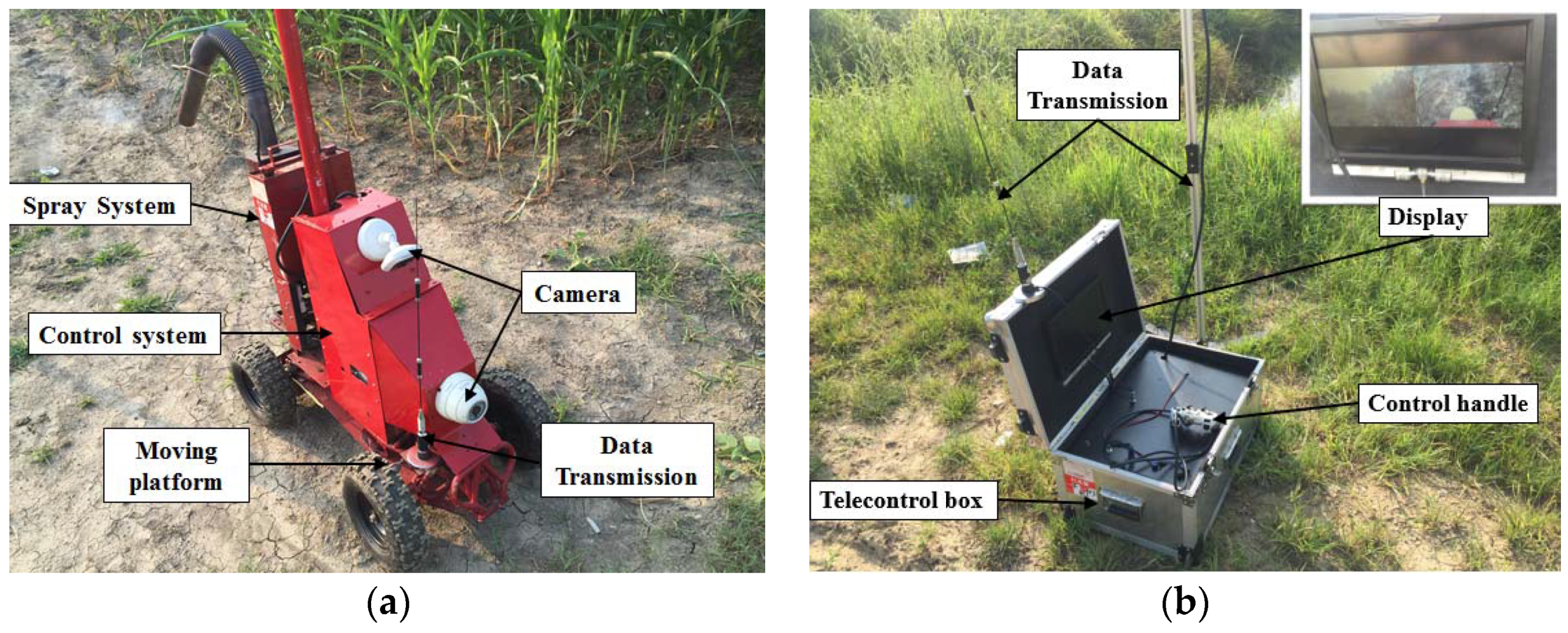
2.1. System Overview

The requirements for the design of the machine platform depend on its environment and purpose, as shown in Figure 1. In the late growth stage of corn, the machine must enter the field for pest and disease control. Following the distance between two rows of corn planted at the maximum acceptable range of 60–80 cm, this article designs an autonomous moving and spraying robot. The autonomous moving and spraying robot consists of three parts: the image acquisition and transmission system, the control platform, and the moving and spraying execution system. The purpose of image acquisition is to collect the front area data to be traversed by the vehicle. After applying the codec for video networking via a wireless bridge (Breeze NET DS802.11, Version 4.1, Alvarion Technologies Ltd., Rosh Ha’ayin, Israel, 2003), the image data are transferred to the control platform. The control platform mainly consists of the Industrial Personal Computer (IPC), signal transmitting and receiving system, and display components.

Path planning is based on the camera’s capacity for detection through the corn stalks, the calibration of the camera to calculate the relative coordinates of the corn on the ground, and its capacity to calculate the most appropriate path for the vehicle to pass. This paper first presents the calibration of the camera in relation to the ground reference plane and the correspondence of the calibration between the images and ground coordinates. Next, the paper presents image acquisition, identification of stalk images, and calculation of the stalk on the ground plane. Finally, the study solves the trajectory path algorithm using the radial basis function (RBF) by the coordinates of stalks on the ground.

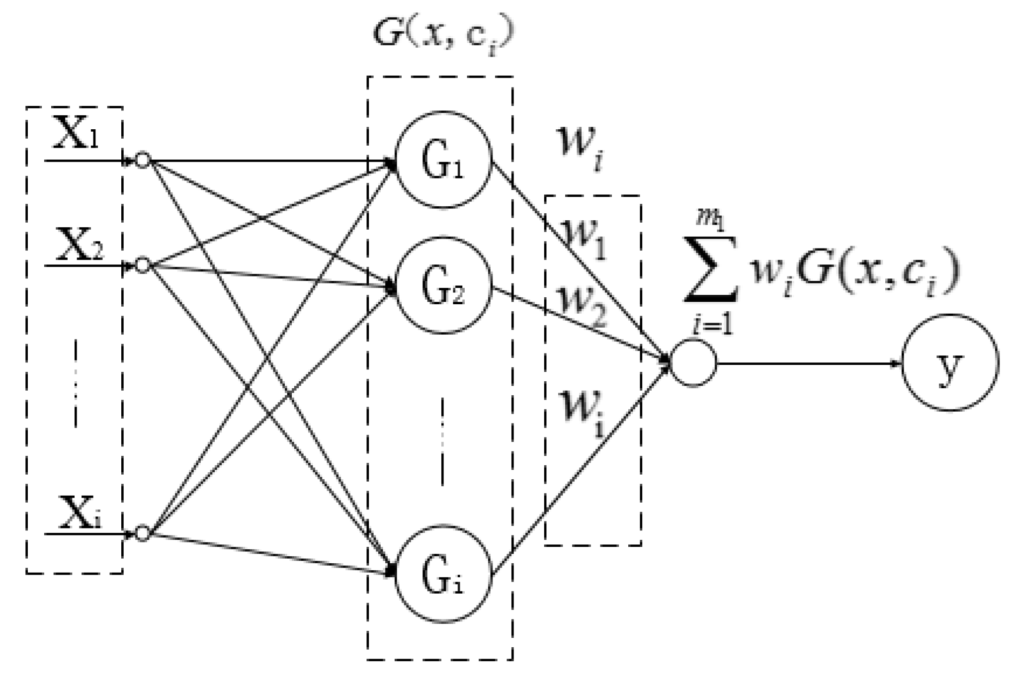
2.2. Navigation Method

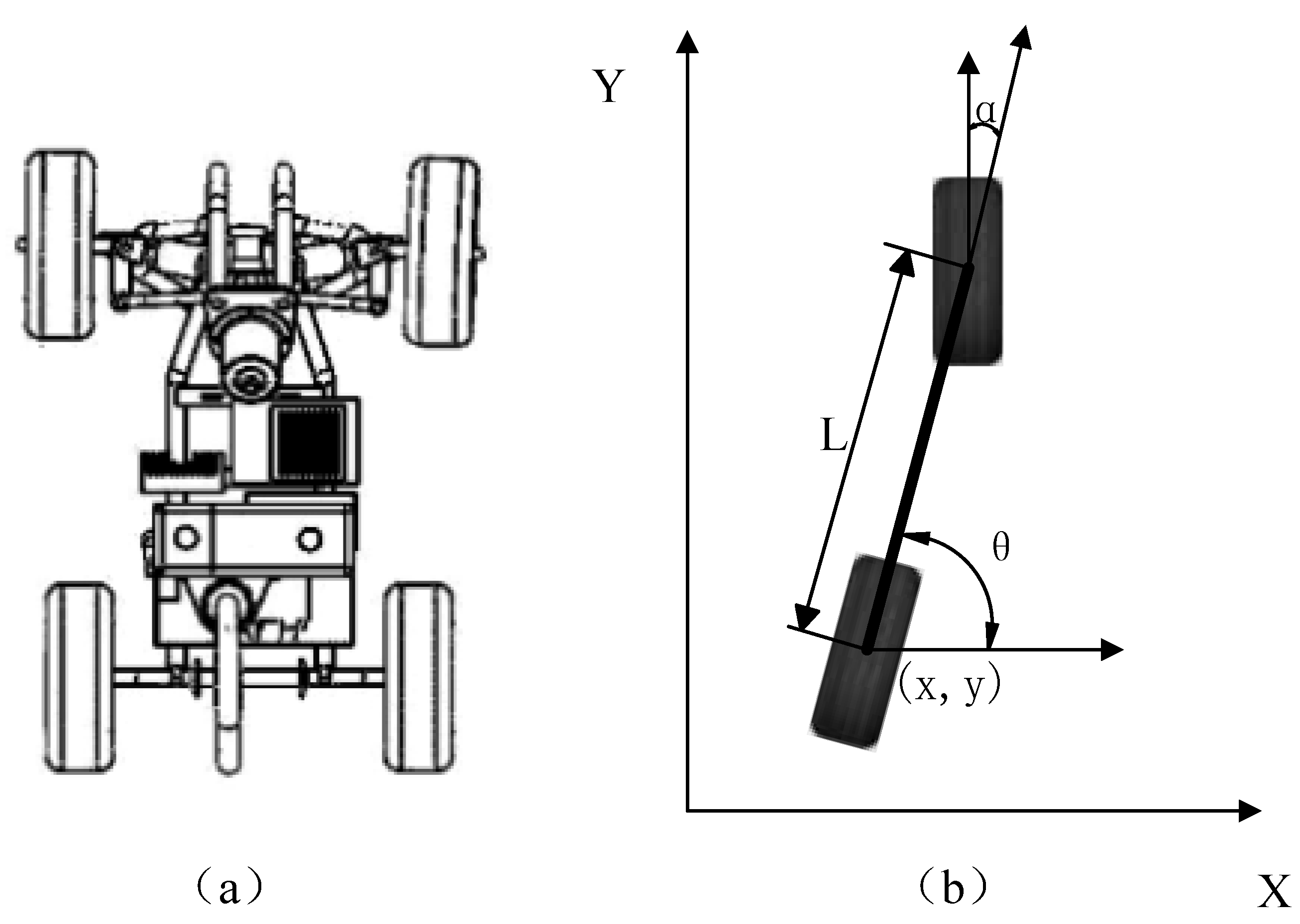
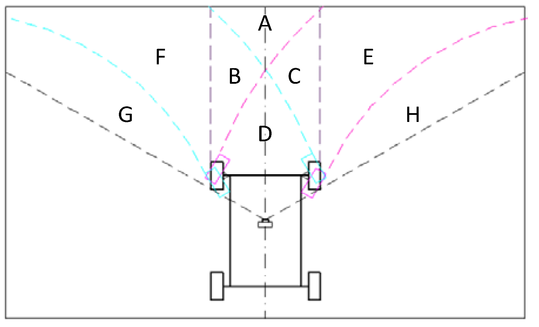
2.2.1. Vehicle Kinematic Model

The execution platform for the mobile sprayer is a typical Ackerman coordinate mobile platform. The two front wheels of the vehicle are steering wheels, and the rear wheels are driving wheels. According to the vehicle kinematics, the movement of the vehicle can be simplified as a bicycle model (as Figure 2b shown) [29]. The kinematics model of vehicle is as follows:

$$\left[\begin{array}{c}\dot{x}\\ \dot{y}\\ \dot{\theta }\end{array}\right]=\left[\begin{array}{c}cos\theta \\ sin\theta \\ \frac{tan\theta }{L}\end{array}\right]\upsilon$$

(1)

where (x, y) are the coordinates of the simplified model of the rear-wheel axle, α is angle of the front wheel and the direction of the vehicle, θ is the angle between the body and the X-axis, and L is the distance between the front and rear axles.

The specifications of the vehicle are shown as follows. The length L is 1.1 m. In addition, the minimum speed (${\upsilon }_{\text{min}}$) is 0 m/s, the maximum speed (${\upsilon }_{\text{max}}$) is 2 m/s. The maximum steering angle ($\phi$) is 26°, and the maximum steering acceleration ($\dot{\phi }$) is 60°/s.

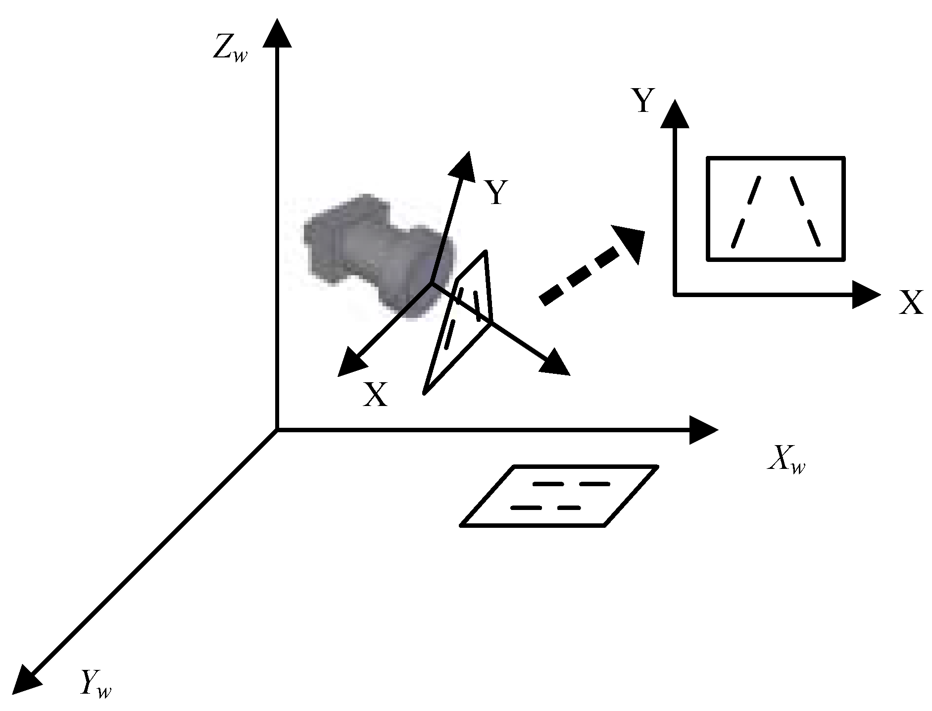
2.2.2. Camera Calibration

Images are captured via a DFK 22AUC03 camera, the Imaging Source Company, Bremen, Germany, with a resolution of 640 × 480 pixels and a shooting frame rate of 87 s⁻¹. The camera and IPC communication are connected via an Ethernet port. The IPC uses a 2.00 GHz Intel processor, with a memory capacity of 4 GB. The camera is installed on the nose of the vehicle, and the photographing direction coincides with the vehicle moving direction. As depicted in Figure 3, the image coordinates and the world coordinates are different. The acquisition of the original image is shown in Figure 4a. The camera imaging principle is used for the calibration of the camera. Due to the camera's imaging principle, objects on the ground could be mapped to the camera plane. The calibration process of the camera obtains the 3D transformation matrix H. Equation (2) shows the calibrated world coordinates and the corresponding image coordinates of the points on the ground. The normalized transformation matrix can be obtained by solving the linear equations using the least-squares method. Calibration of the camera is calculated by the camera point captured image and positions by LIDAR collection in the world coordinate system, as Figure 4.

$$\left[\begin{array}{l}x\\ y\\ z\end{array}\right]=H\left[\begin{array}{l}{x}_w\\ y_w\\ 1\end{array}\right]$$

(2)

where (x, y) denote the image coordinates and (x_w, y_w) denote the world coordinate system.

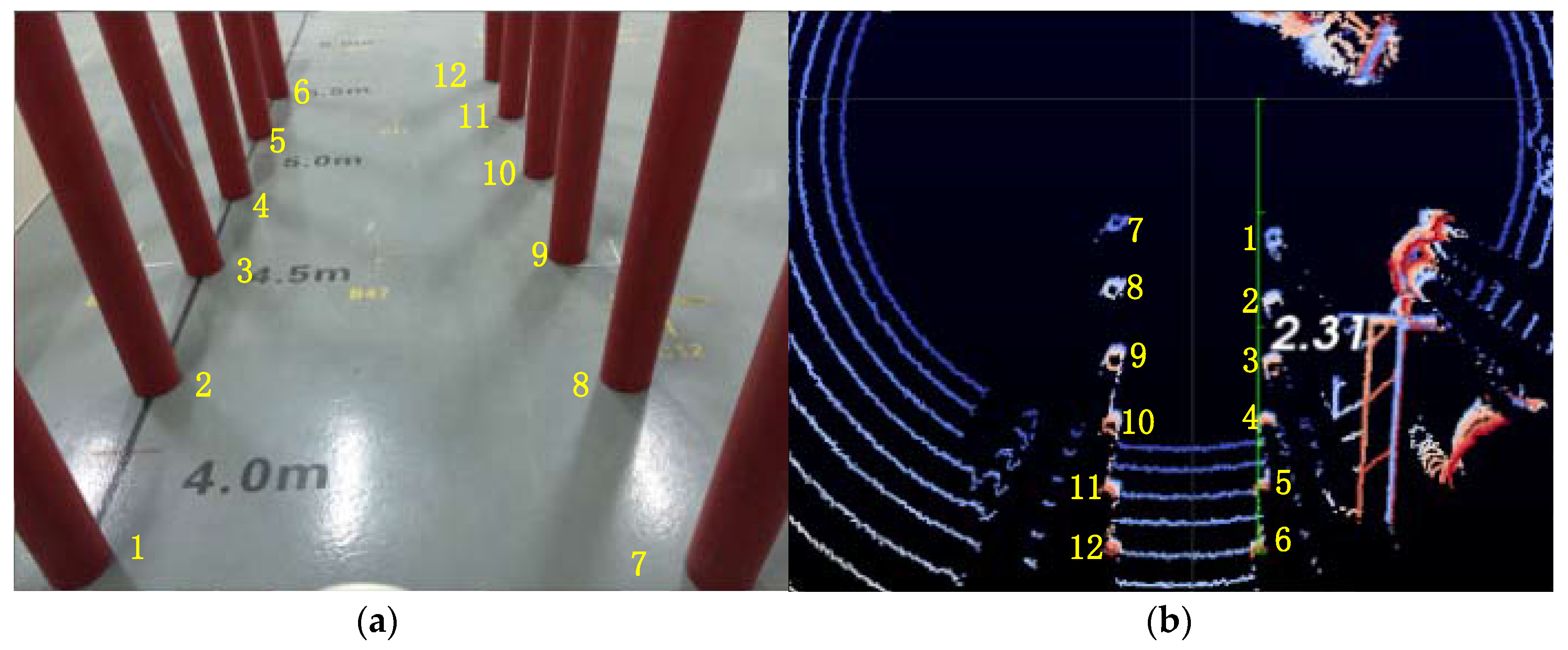
2.2.3. Image Recognition

Here, we first explain the vehicle's working environment. The vehicle moves between the crop rows. There is about a 70 cm gap between crop rows, and the width of the vehicle is about 55 cm, as Figure 5 shows. In ideal conditions, clearances on both sides of the vehicle are about 5–8 cm. Figure 6 shows the division of the area in front of the vehicle. When A, B, C, D regions have no stalk, it can be passed easily. When F and C (or B and E) regions have stalks, then the vehicle processes through a complex path planning method, so that the vehicle may bypass the C area (B area) of crops, and finally return to the correct crop row. Conventional agriculture monocular vision navigation methods often use a method of extracting straight crop rows. First, we can find the boundary of the passable area between rows by using the image segmentation method. Then, the center line as a navigational index can be calculated. This method has larger error, ignoring crops outside the crop row, resulting in collision between the vehicle and crops. In addition, navigating along this line in such a high density planting will result in larger heading deflection, so that the next frame of the navigational index extraction error increases. Therefore, in such a confined environment it is necessary to extract the navigational index to identify all of the stalks, find a path with the smallest collision probability from all of the stalks, and reduce the change of heading.

Image recognition is realized mainly through the following steps:

(i)

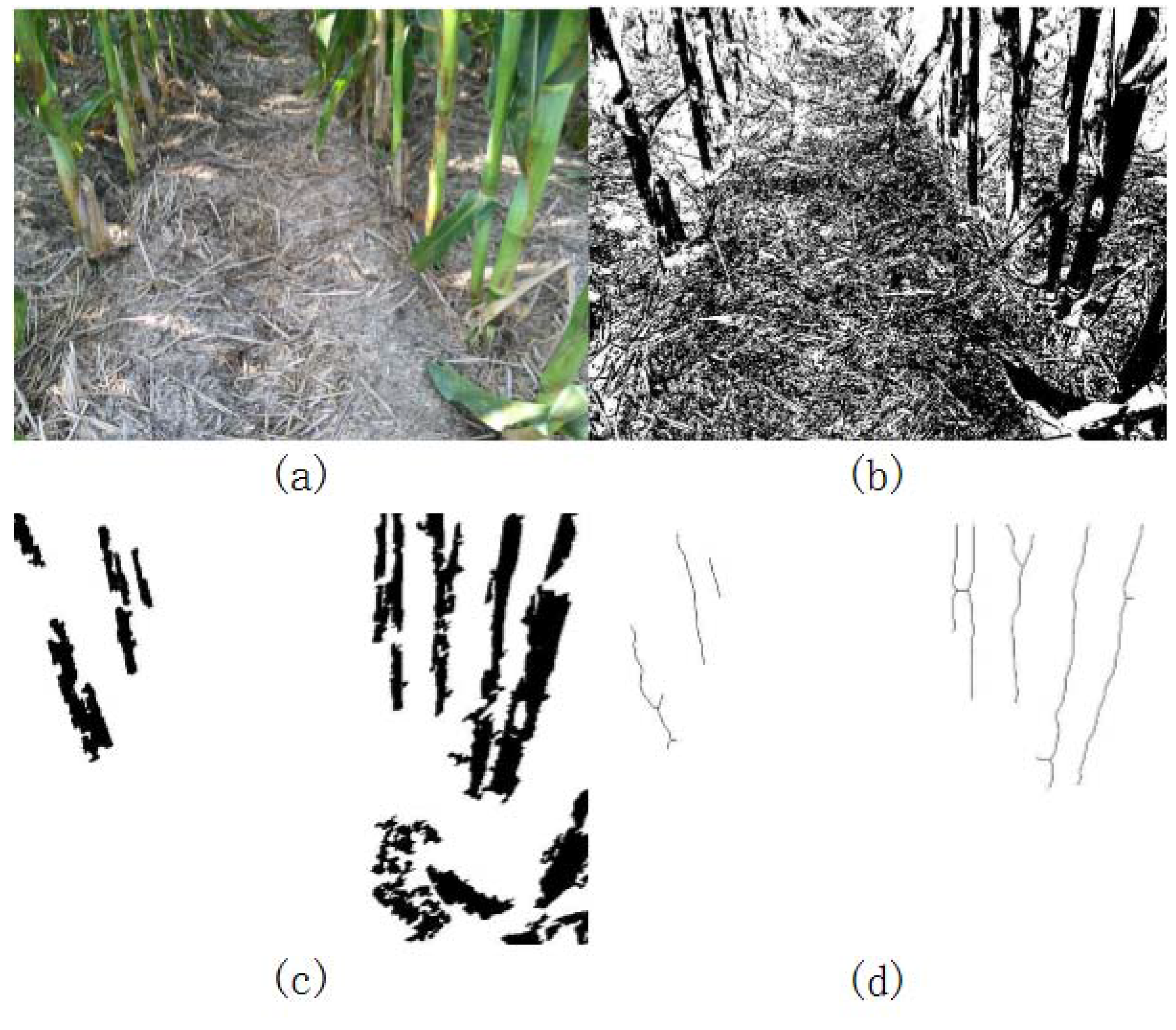
RGB threshold analysis: the target stalk image region and other regional RGB values are separated, and the threshold range image is determined.

(ii)

Otsu threshold analysis: this study uses the Otsu algorithm for image binarization. The threshold of the method is used to maximize the class variance between the foreground and background. This method is very sensitive to noise and target size and has better image segmentation results for the variance between two classes of a unimodal image, as shown in Figure 7.

(iii)

Analysis of the image block filter: the domain neighbor segmentation method is used to filter out noise points caused by the binarization processing of the weeds and corn stubble of the previous quarter image:

$$N_4=(x,y)\cup (x,y-1),(x+1,y),(x,y+1),(x-1,y)$$

(3)

The area of each connected region of the image is calculated through the method of neighbor domains, according to the area in descending order. The image blocks are less than 50 pixels, by experience, which is regarded as the standard for noise elimination.

After removing the isolated noise points, the interference of weeds and other extracted stalks is filtered out. However, maize leaves and weeds are similar to the stalk in the image block, and they still cause significant interference in the recognition of stalks. As Figure 7b shows, the shapes of maize leaves and weeds are irregular, but that of stalks is elongated.

The system uses tiles of an external rectangular box for further noise removal. All of the tiles of the circumscribed rectangles are obtained, and the aspect ratio of the external rectangle is used as the basis for assessment. An aspect ratio greater than five is marked as the maize stalk, and the other shapes are defined as noise. In Figure 7c, the solid black image represents the stalk, and the hollow block represents the noise to be removed. In Figure 7d, the stalk independently calculated for each block is used to extract the ridge line. The lowest point of the ridge line is marked as the coordinate point of each stalk.

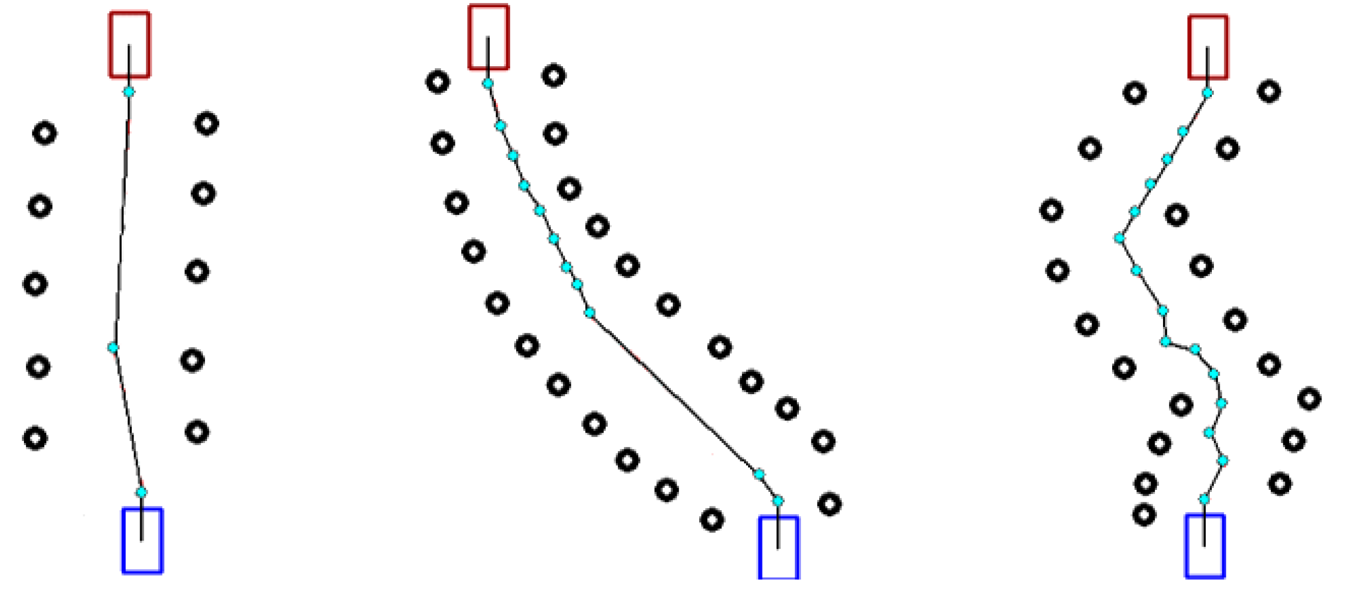
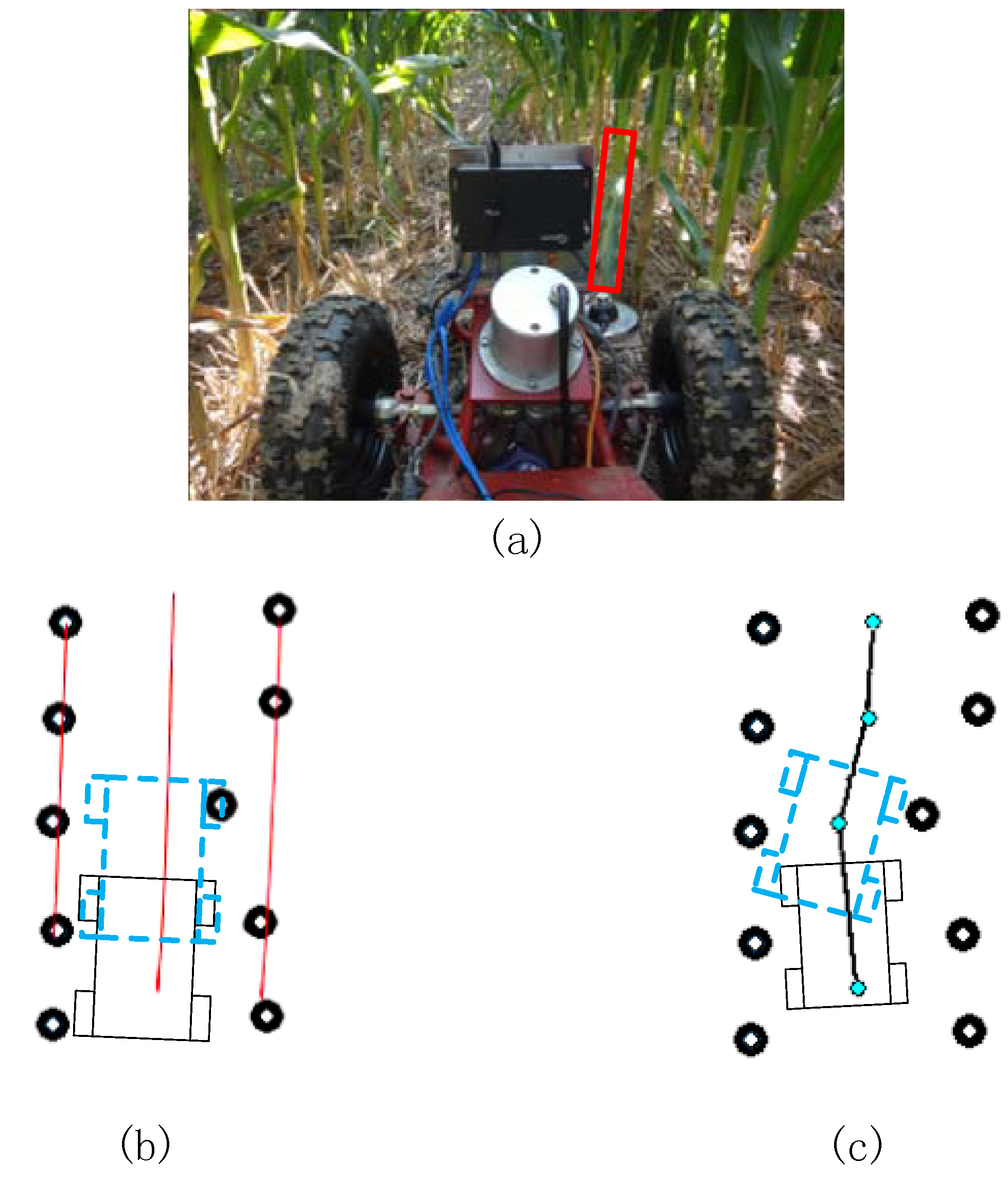
2.2.4. Detection of the Crop Row Line

Many stalks of corn, given a number of man-made or natural factors, are not in the corn row. Trajectory planning by the system is needed to navigate the vehicle. The optimal trajectory based on the global map has been widely studied in the field of robot navigation [30,31,32]. The coordinate points of all stalks are mapped in accordance with the world coordinate. Among the methods of agricultural machinery navigation, Hough transform is one of the most commonly used. The results obtained by the Hough transform have larger errors. The RBF, which behaves like a local approximation of the neural network and has many advantages, is used for path planning in the corn fields. It is not susceptible to the problems associated with non-fixed input because of its hidden behavior unit. A regularization method may well reflect the “geometric” features when approaching [33]. The regularization network topology is shown in Figure 8. The RBF network with a nonlinear separable hidden layer first converts the input space into a linearly-separable feature space (usually a high-dimensional space) and then the output layer of the linear division, thereby completing the classification. X = (x₁, x₂ … x_i) is the input data. y = [y₁, y₂ ... y_i]^T is calculated as the final output.

RBF uses a Gaussian radial basis function. The RBF learning algorithm is used to solve the center vector C_i, the width parameter σ_i, and the connection weights between the values of the hidden and output layers ω_i.

$$G(x,c_i)=\text{exp}(-\frac{m_1}{d_{\text{max}}^2}{\Vert x-c_i\Vert }^2)\hspace{1em}\mathit{i}=1, 2 \dots m_1$$

(4)

where m₁ is the number of centers, and d_max is the maximum distance between the selected centers. As can be seen, all of the standard deviations are fixed to ensure that each RBF are not too sharp, nor too shallow:

$$\mathsf{\sigma }=\frac{d_{\text{max}}}{\sqrt{2m_1}}$$

(5)

The inputs of the hidden layer are the combinations of the input vector x = [x₁, x₂ … x_n]^T. The network of the hidden layer to the output layer is linearly mapped:

$$y={\displaystyle \sum _{i=1}^{m_1}{w}_{i}G(x,c_i)}$$

(6)

Finally, the availability of the Gaussian kernel network structure is given by:

$$y={\displaystyle \sum _{i=1}^k{w}_i\exp (-{\Vert x-u_i\Vert }^2/2{\sigma }_i^2)}$$

(7)

In this article, a term which constrains the complexity of the approximation function is added based on the standard error term:

$$e=d_k-y$$

(8)

where $d_k$ is the distance between the selected centers for the sample of k.

The Gaussian basis function is local to the center vector, in the sense that:

$$\underset{\Vert x\Vert \to \infty }{\lim }\rho \Vert x-u_i\Vert =0$$

(9)

In this study, n is the number of centers, and d is the maximum distance between the chosen centers. Thus:

$$\sigma =\frac{d_{}}{\sqrt{2n}}$$

(10)

The smaller the value of d, the smaller the width of RBF and, therefore, the more selective the base function is. In a regularization network, the number of hidden behavior units is the same as the sample, and the data center of the basis function is the sample itself. The extension function and the connection weights are the only parameters that were taken into account.

Stalk coordinates correspond with the world coordinate as the input for online learning. With a gradient of training methods, the learning rate was 0.001, and the target error was 0.05. While the error is less than 0.05, the network outputs the result G(x, c_i); otherwise, it adds a set to the sample. It can adapt well to the complex diversity of the vehicle environmental planning exercise with a $\mathsf{\sigma }$ value of 0.3. RBF results are similar to high-order polynomial fitting, but smoother for the traveling environment of the vehicle.

Figure 9 shows an experimental scenario with a crop outside the crop row; the outlier identified by the red box deviates from the crop rows by about 6 cm, comparing path trajectories calculated between the centerline extraction method and RBF. Using the centerline extraction method, although the navigation line is offset to the left in this situation, the probability of collision by the vehicle and the outlier stalk is very high, due to the width of the vehicle. However, using the RBF method, where there is a heading angle of deflection, the vehicle pass rate has been increased significantly.

3. Experimental and Discussion

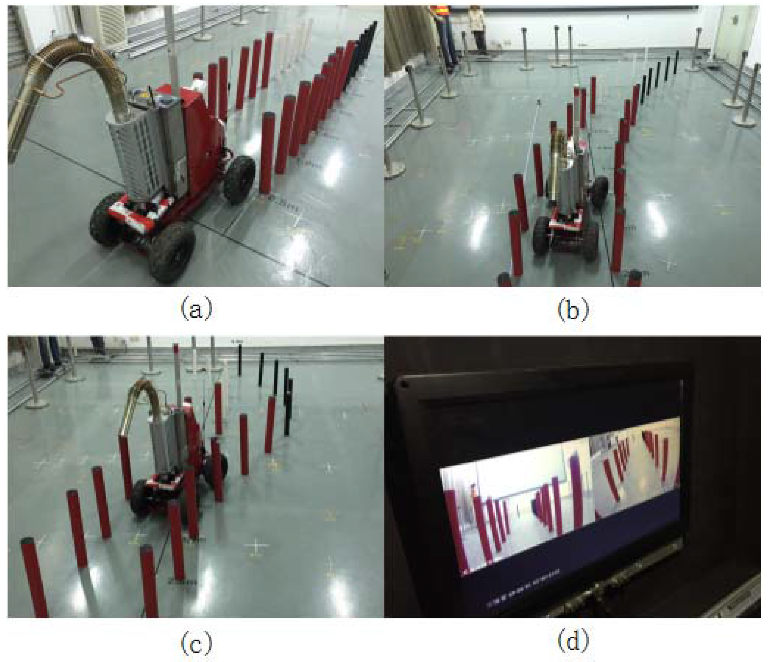
3.1. Laboratory Tests

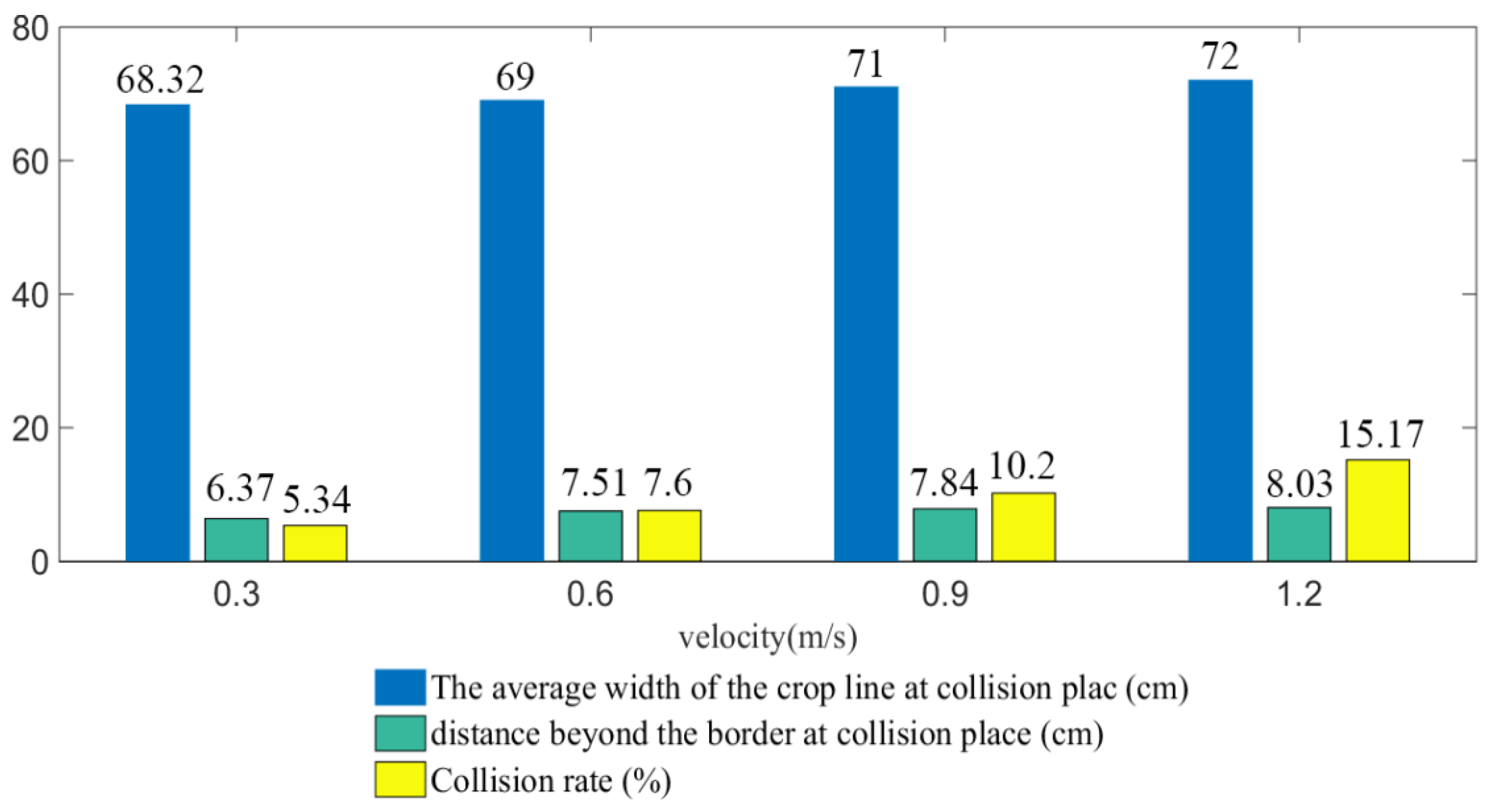
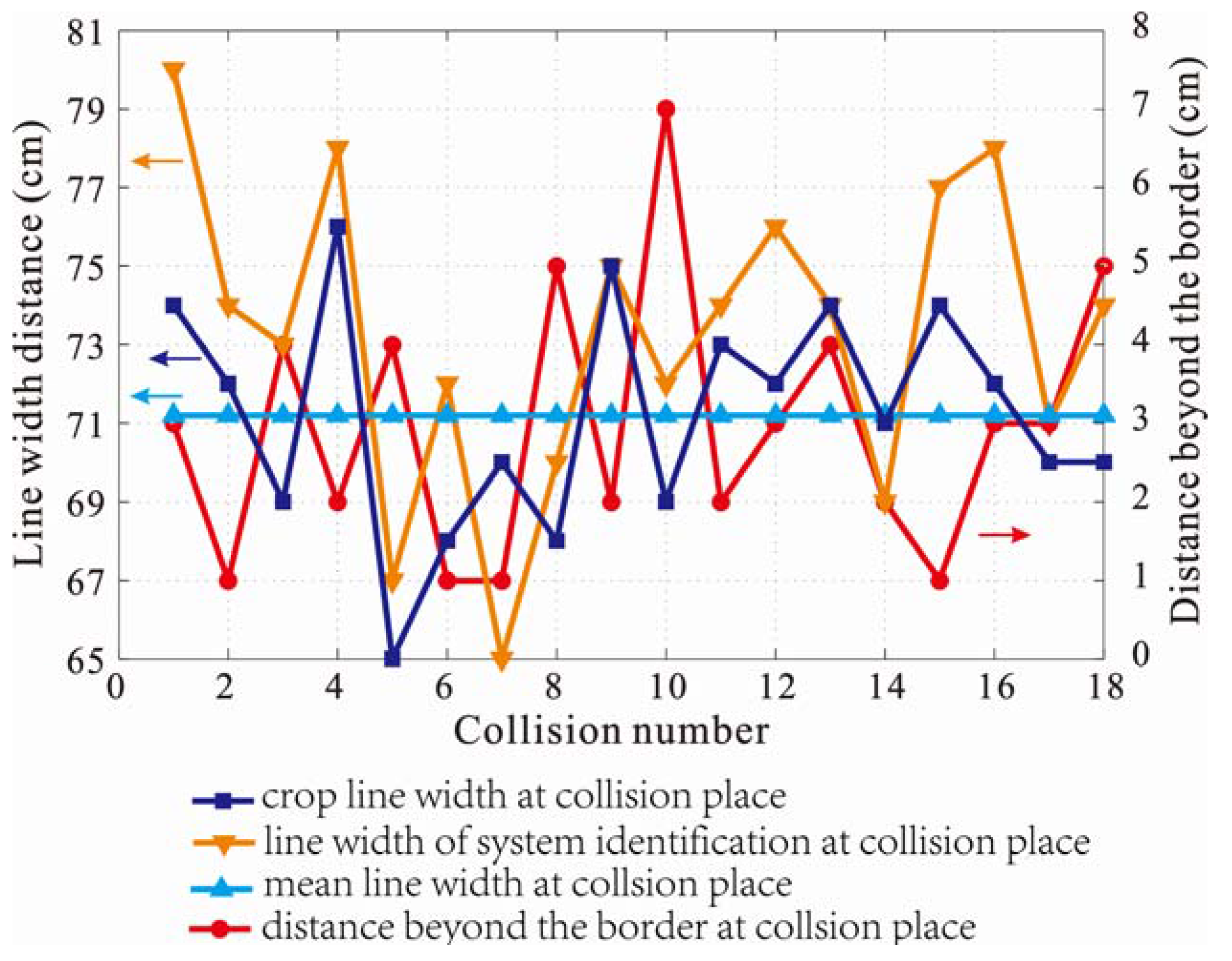
This study conducted laboratory tests and field trials to test the performance of the robot in terms of the path detection and planning system. Laboratory tests were conducted at the Chinese Academy of Sciences under different path characteristics. RBF path planning simulation was conducted, and the verification results are obtained as shown below. In Figure 10, the front of the vehicle, both left and right sides, are placed with separate columns, and the columns of the same row have a spacing of 10 cm to 15 cm. The spacing between two rows is in a range of 65, 70, and 75 cm, and the rows are intentionally placed in a straight line path, left-turn, right-turn, and S-turn. The vehicle speed is set at 0.3–1.3 m/s with a velocity increment of 0.2 m/s. Any instance of the vehicle crashing into a post, as it passes through the post area at various speeds, is recorded, and the speed of path planning is analyzed and optimized.

Figure 11 shows the simulation results of the RBF method for straight line, left-turn, and S-turn. It is easy to obtain in a non-linear case; the vehicle path planning by the RBF method was more reasonable for collision avoidance in a confined space.

A number of simulations were conducted in the laboratory to demonstrate the applicability of the approach in different shapes of crop rows, such as straight line, left-turned, right-turned, and S-bent. All of the paths are accessible, with a width of 65–75 cm, and the vehicle has an operating width of 60 cm. As listed in

Table 1. Test comparison of indoor path planning method.

Velocity	RBF (%)				Hough Transform (%)
m/s	Straight	Left Turn	Right Turn	S-Turn	Straight	Left Turn	Right Turn	S-Turn
0.3	0.00	0.03	0.07	0.17	0.00	0.13	0.17	0.30
0.5	0.00	0.10	0.07	0.20	0.00	0.17	0.13	0.33
0.7	0.00	0.07	0.10	0.13	0.00	0.17	0.20	0.43
0.9	0.03	0.13	0.07	0.20	0.00	0.27	0.27	0.43
1.1	0.00	0.10	0.13	0.23	0.00	0.30	0.33	0.50
1.3	0.07	0.10	0.10	0.27	0.03	0.40	0.37	0.60

, after correcting the direction of the body, almost no extra steering action occurs in the straight path, a speed of 0.3–1.3 m/s is successfully achieved. However, in the left-turned and right-turned paths, increasing the speed increases the chances of a collision. In addition, the results of RBF are more significantly improved than those of Hough transform in an S-bent path. In particular, when the turning radius changes, the calculations for the front and rear frames do not always fully coincide, resulting in deviations in the execution of the vehicle, which are likely to cause collision with the columns. Overall, in the case of a changing turning radius, the rate of vehicle and column collision is below 27% under the RBF algorithm.

In response to these four scenarios, respectively, the Hough transform algorithm and simplified RBF algorithm performed each plan 10 times, and the average search time and the minimum distance of the boundary results were compared. As shown in the

Table 2. The average search time and the minimum distance of the boundary by Hough and RBF.

Algorithm	Straight		Left-Turn		Right-Turn		S-Turn
	Time (ms)	L (cm)	Time (ms)	L (cm)	Time (ms)	L (cm)	Time (ms)	L (cm)
Hough	25.16	25.4	25.70	22.7	25.76	21.5	26.31	16.4
RBF	28.07	27.6	30.64	26.3	30.22	27.7	31.40	28.1

L: The minimum distance to the boundary.

below, calculations using the Hough transform time are faster than the average RBF by about 3–5 ms; however, the minimum distance to the boundary of the RBF is significantly better than the results of Hough transform.

3.2. Field Trials

A few field trials were conducted in the Longkang Farms of Guoyang, Anhui Province, China in July and August, 2015, shown in Figure 12. In the field tests, six different lines were randomly selected as lanes, and the passage of the vehicle in the cornfield was detected through image recognition and path planning. The test line had a length of 100 m, and the crop rows, which were organized using the segmented measurement method, had a width of 60 to 80 cm. The vehicle autonomously navigated the field using the camera. The speed of the vehicle was set to 0.3–1.2 m/s, with a velocity increment of 0.3 m/s. The collision rate, the width of the row at the collision position, and the distance of the vehicle beyond the boundaries of the row were recorded during the testing of the vehicle through the test area. The average image processing time, including network latency, is 220 ms, which meets the maximum 2 m/s speed of the vehicle. In this system, due to the limitation of range capacity and power consumption of the system, images acquired are sent to the control platform wirelessly. The average image processing time includes network latency. The wireless bridge maximum power is 800 mW. Furthermore, the crop has a certain blocking effect on signal transmission, a delay time that cannot be ignored. By measuring in the corn field, transmission delay is about 100–150 ms on average for 100 m distance. The speed of processing satisfies the speed of the vehicle moving in the field.

The majority of the maize was planted mechanically and the remainders were planted manually. Thus, the operating line in most of the area is almost a straight path, and some parts of the area are not straight. The passage of the vehicle through 100 m operating lines of four test columns was recorded, as well as its collision rates, the width of the crop row in collision, and the robot collision in the field beyond the distance of the boundary.

Figure 13 shows a histogram of the stability of the system in the case of a vehicle running at different speeds. In all cases, the stability of the system decreases with increasing speeds. When the speed is too fast, the response of the system cannot meet the needs of the vehicle, and the response time of the algorithm entails higher requirements. The experiments showed that the efficiency of the vehicle, road conditions (e.g., width of the workspace and weeds between the crops), and system responsiveness have positive effects.

As shown in

Table 3. The results of collision rate test.

Collision Number	The Total Number of Maize	The Number of Collisions with Robot	Collision Rate	The Average Line Width (cm)	The Average Line Width of Collision (cm)	Distance Beyond the Border at Collision Place (cm)
1	357	18	5.04%	74.5	68.1	5.8
2	329	21	6.38%	72.8	67.4	6.4
3	336	19	5.65%	74.2	68.8	7.2
4	341	16	4.69%	76.4	69.0	6.1
SUM	1363	74	5.43%	-	-	-

, four trials were conducted on the statistical data with a speed of 0.6 m/s. The collision rates were 5.04%, 6.38%, 5.65%, and 4.69%, and the average probability of a vehicle collision with stalks was 4.3%. The first group of data into Figure 13 was analyzed.

Figure 14 shows the crops in the event of a crash test of a collision with the wide row crops, as well as the collision at a distance beyond the crop rows.

(i)

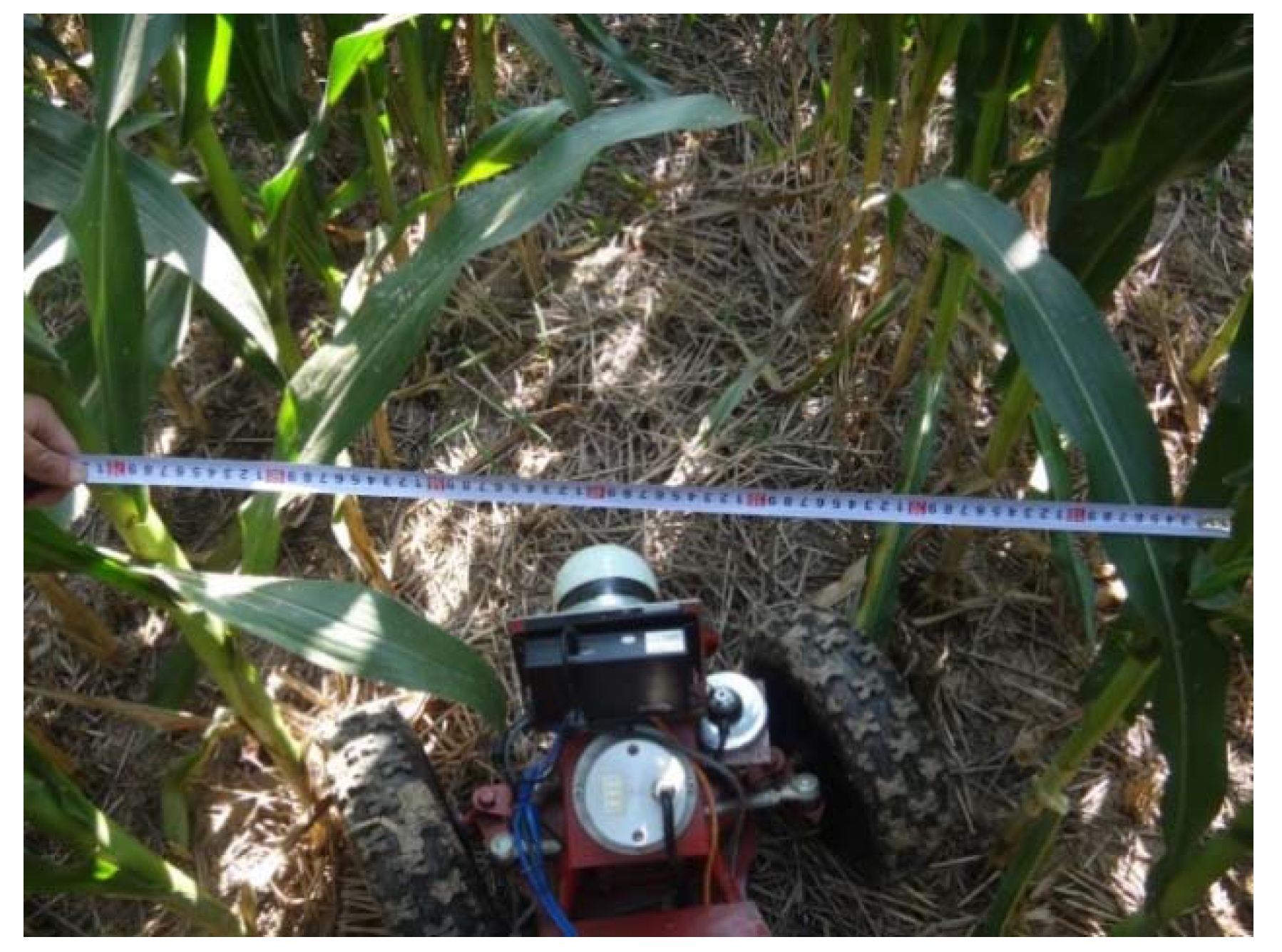
When the line width is small, the possibility of a vehicle collision with stalks is very high. For example, for the collision with an average row width of 68 cm, the actual measured line width is 74 cm.

(ii)

When the system inaccurately recognizes the root position above the ground, it can easily lead to a collision between the vehicle and stalk.

(iii)

For the crop density, when the vehicle drives through a sparsely planted area, collision is likely.

4. Conclusions

A new monocular visual navigation method for long-stalked crops is studied and proposed. One camera is used to collect images of crop distribution in front of the vehicle. Stalk image information is obtained by using color threshold analysis and morphological classification. The RBF method is utilized to obtain an optimized trajectory between rows of stalks. As shown in Figure 9, the trajectory planned by RBF methods is much smoother than the one planned by Hough methods. This method has significant advantages for non-straight paths.

The new method is tested, and the results show that it can significantly improve the trafficability and maneuverability in long-stalked crop fields. As shown in the experiments, when the vehicle operates at a normal speed (0.7 m/s), the collision rate with stalks are under 6.38% in a cornfield. The results also show that the vehicle passes smoothly through tall crops via this method. The response period of the algorithm needs to be furtherly reduced, and the positioning accuracy of the vision needs to be improved in future research.

References

1. Bochtis, D.D.; Sørensen, C.G.C.; Busato, P. Advances in agricultural machinery management: A review. Biosyst. Eng. 2014, 126, 69–81. [Google Scholar] [CrossRef]
2. Mathanker, S.K.; Grift, T.E.; Hansen, A.C. Effect of blade oblique angle and cutting speed on cutting energy for energycane stems. Biosyst. Eng. 2015, 133, 64–70. [Google Scholar] [CrossRef]
3. Qi, L.; Miller, P.C.H.; Fu, Z. The classification of the drift risk of sprays produced by spinning discs based on wind tunnel measurements. Biosyst. Eng. 2008, 100, 38–43. [Google Scholar] [CrossRef]
4. Tillett, N.D.; Hague, T.; Grundy, A.C.; Dedousis, A.P. Mechanical within-row weed control for transplanted crops using computer vision. Biosyst. Eng. 2008, 99, 171–178. [Google Scholar] [CrossRef]
5. Vidoni, R.; Bietresato, M.; Gasparetto, A.; Mazzetto, F. Evaluation and stability comparison of different vehicle configurations for robotic agricultural operations on side-slopes. Biosyst. Eng. 2015, 129, 197–211. [Google Scholar] [CrossRef]
6. Suprem, A.; Mahalik, N.; Kim, K. A review on application of technology systems, standards and interfaces for agriculture and food sector. Comput. Stand. Interfaces 2013, 35, 355–364. [Google Scholar]
7. Cordill, C.; Grift, T.E. Design and testing of an intra-row mechanical weeding machine for corn. Biosyst. Eng. 2011, 110, 247–252. [Google Scholar] [CrossRef]
8. Bochtis, D.; Griepentrog, H.W.; Vougioukas, S.; Busato, P.; Berruto, R.; Zhou, K. Route planning for orchard operations. Comput. Electron. Agric. 2015, 113, 51–60. [Google Scholar] [CrossRef]
9. Pérez-Ruiz, M.; Gonzalez-de-Santos, P.; Ribeiro, A.; Fernandez-Quintanilla, C.; Peruzzi, A.; Vieri, M.; Tomic, S.; Agüera, J. Highlights and preliminary results for autonomous crop protection. Comput. Electron. Agric. 2015, 110, 150–161. [Google Scholar] [CrossRef]
10. Aldo Calcante, F.M. Design, development and evaluation of a wireless system for the automatic identification of implements. Comput. Electron. Agric. 2014, 2014, 118–127. [Google Scholar] [CrossRef]
11. Balsari, P.; Manzone, M.; Marucco, P.; Tamagnone, M. Evaluation of seed dressing dust dispersion from maize sowing machines. Crop Prot. 2013, 51, 19–23. [Google Scholar] [CrossRef]
12. Gobor, Z.; Lammer, P.S.; Martinov, M. Development of a mechatronic intra-row weeding system with rotational hoeing tools: Theoretical approach and simulation. Comput. Electron. Agric. 2013, 98, 166–174. [Google Scholar] [CrossRef]
13. Bakker, T.; van Asselt, K.; Bontsema, J.; Müller, J.; van Straten, G. Autonomous navigation using a robot platform in a sugar beet field. Biosyst. Eng. 2011, 109, 357–368. [Google Scholar] [CrossRef]
14. Bakker, T.; Wouters, H.; van Asselt, K.; Bontsema, J.; Tang, L.; Müller, J.; van Straten, G. A vision based row detection system for sugar beet. Comput. Electron. Agric. 2008, 60, 87–95. [Google Scholar] [CrossRef]
15. Gan-Mor, S.; Clark, R.L.; Upchurch, B.L. Implement lateral position accuracy under RTK-GPS tractor guidance. Comput. Electron. Agric. 2007, 59, 31–38. [Google Scholar]
16. Åstrand, B.; Baerveldt, A.-J. A vision based row-following system for agricultural field machinery. Mechatronics 2005, 15, 251–269. [Google Scholar] [CrossRef]
17. Chen, B.; Tojo, S.; Watanabe, K. Machine Vision for a Micro Weeding Robot in a Paddy Field. Biosyst. Eng. 2003, 85, 393–404. [Google Scholar] [CrossRef]
18. Billingsley, J.; Schoenfisch, M. The successful development of a vision guidance system for agriculture. Comput. Electron. Agric. 1997, 16, 147–163. [Google Scholar] [CrossRef]
19. Burgos-Artizzu, X.P.; Ribeiro, A.; Guijarro, M.; Pajares, G. Real-time image processing for crop/weed discrimination in maize fields. Comput. Electron. Agric. 2011, 75, 337–346. [Google Scholar] [CrossRef] [Green Version]
20. Meng, Q.; Qiu, R.; He, J.; Zhang, M.; Ma, X.; Liu, G. Development of agricultural implement system based on machine vision and fuzzy control. Comput. Electron. Agric. 2014, 112, 128–138. [Google Scholar] [CrossRef]
21. Xue, J.; Zhang, L.; Grift, T.E. Variable field-of-view machine vision based row guidance of an agricultural robot. Comput. Electron. Agric. 2012, 84, 85–91. [Google Scholar] [CrossRef]
22. Bui, T.T.Q.; Hong, K.-S. Evaluating a color-based active basis model for object recognition. Comput. Vis. Image Underst. 2012, 116, 1111–1120. [Google Scholar]
23. Bui, T.T.Q.; Hong, K.-S. Extraction of sparse features of color images in recognizing objects. Int. J. Control Autom. Syst. 2016, 14, 616–627. [Google Scholar]
24. Gée, C.; Bossu, J.; Jones, G.; Truchetet, F. Crop/weed discrimination in perspective agronomic images. Comput. Electron. Agric. 2008, 60, 49–59. [Google Scholar] [CrossRef]
25. Guerrero, J.M.; Pajares, G.; Montalvo, M.; Romeo, J.; Guijarro, M. Support Vector Machines for crop/weeds identification in maize fields. Expert Syst. Appl. 2012, 39, 11149–11155. [Google Scholar] [CrossRef]
26. Montalvo, M.; Guerrero, J.M.; Romeo, J.; Emmi, L.; Guijarro, M.; Pajares, G. Automatic expert system for weeds/crops identification in images from maize fields. Expert Syst. Appl. 2013, 40, 75–82. [Google Scholar] [CrossRef]
27. Zhang, J.; Kantor, G.; Bergerman, M. Monocular visual navigation of an autonomous vehicle in natural scene corridor-like environments. In Proceedings of the IEEE/RSJ International Conference on Intelligent Robots and Systems (IROS), Vilamoura, Portugal, 7–12 October 2012; IEEE: Piscataway, NJ, USA; pp. 3659–3666.
28. Montalvo, M.; Pajares, G.; Guerrero, J.M.; Romeo, J.; Guijarro, M.; Ribeiro, A.; Ruz, J.J.; Cruz, J.M. Automatic detection of crop rows in maize fields with high weeds pressure. Expert Syst. Appl. 2012, 39, 11889–11897. [Google Scholar] [CrossRef] [Green Version]
29. Du, M.; Mei, T.; Liang, H.; Chen, J.; Huang, R.; Zhao, P. Drivers’ Visual Behavior-Guided RRT Motion Planner for Autonomous On-Road Driving. Sensors 2016, 16, 102. [Google Scholar] [CrossRef] [PubMed]
30. Bui, T.T.Q.; Hong, K.-S. Sonar-based obstacle avoidance using region partition scheme. J. Mech. Sci. Technol. 2010, 24, 365–372. [Google Scholar]
31. Pamosoaji, A.K.; Hong, K.-S. A path planning algorithm using vector potential functions in triangular regions. IEEE Trans. Syst. Man Cybern. Syst. 2013, 43, 832–842. [Google Scholar] [CrossRef]
32. Tamba, T.A.; Hong, B.; Hong, K.-S. A path following control of an unmanned autonomous forklift. Int. J. Control Autom. Syst. 2009, 7, 113–122. [Google Scholar] [CrossRef]
33. Chen, J.; Zhao, P.; Liang, H.; Mei, T. Motion planning for autonomous vehicle based on radial basis function neural network in unstructured environment. Sensors 2014, 14, 17548–17566. [Google Scholar] [CrossRef] [PubMed]
Figure 1. The system of the moving vehicle. (a) The moving and spraying execution system; and (b) the control platform.
Applsci 06 00182 g001
Figure 2. Mobile platform model and simplified model for kinematics. (a) Mobile platform model; and (b) simplified model for kinematic.
Applsci 06 00182 g002
Figure 3. Transformation between the world coordinate and the camera coordinate.
Applsci 06 00182 g003
Figure 4. Transformation between data from the image and LIDAR. (a) Image points in camera coordinates; and (b) absolute coordinates in the world coordinate system.
Applsci 06 00182 g004
Figure 5. The vehicle’s moving environment.
Applsci 06 00182 g005
Figure 6. The division of the area in front of the vehicle.
Applsci 06 00182 g006
Figure 7. (a) The original image; (b) the results of Otsu threshold analysis; (c) the results of a block filter; and (d) the results of extracting the ridge line.
Applsci 06 00182 g007
Figure 8. Regularization network structure.
Applsci 06 00182 g008
Figure 9. Comparison between centerline extraction method and RBF for crops outside the crop rows, (a) experimental scenario; (b) result of centerline extraction algorithm; and (c) result of RBF.
Applsci 06 00182 g009
Figure 10. Laboratory tests: (a) straight line; (b) right-turn; (c) S-turn; and (d) the display of the front camera.
Applsci 06 00182 g010
Figure 11. Results of path planning by RBF.
Applsci 06 00182 g011
Figure 12. Testing of fogging machine in the field.
Applsci 06 00182 g012
Figure 13. A histogram of the stability of the system in the case of a vehicle running at different speeds.
Applsci 06 00182 g013
Figure 14. The stalk width and identification width of the collision position.
Applsci 06 00182 g014