On Site Investigation and Health Monitoring of a Historic Tower in Mantua, Italy

Abstract

The paper describes the strategy adopted to assess the structural condition of the tallest historic tower in Mantua (Italy) after the Italian seismic sequence of May–June 2012 and exemplifies the application of health monitoring using (automated) operational modal analysis. The post-earthquake survey (including extensive visual inspection, historic and documentary research, non-destructive (ND) material testing, and ambient vibration tests) highlighted the poor state of preservation of the upper part of the tower; subsequently, a dynamic monitoring system (consisting of a few accelerometers and one temperature sensor) was installed in the building to address the preservation of the historic structure, and automated modal identification was continuously performed. Despite the low levels of vibration that existed in operational conditions, the analysis of data collected over a period of about 15 months allowed to assess and model the effects of changing temperature on modal frequencies and to detect the occurrence of abnormal behavior and damage under the changing environment. The monitoring results demonstrate the potential key role of vibration-based structural health monitoring, implemented through low-cost hardware solutions and appropriate software tools, in the preventive conservation and the condition-based maintenance of historic towers.

1. Introduction

The Italian seismic sequence of May–June 2012 [1] highlighted the high vulnerability of the historical architectures, especially in the southern part of the province of Mantua and in the neighboring Emilia-Romagna region, where several brittle collapses of towers, fortification walls, and castles occurred [2,3], despite the supposed low seismicity of the area.

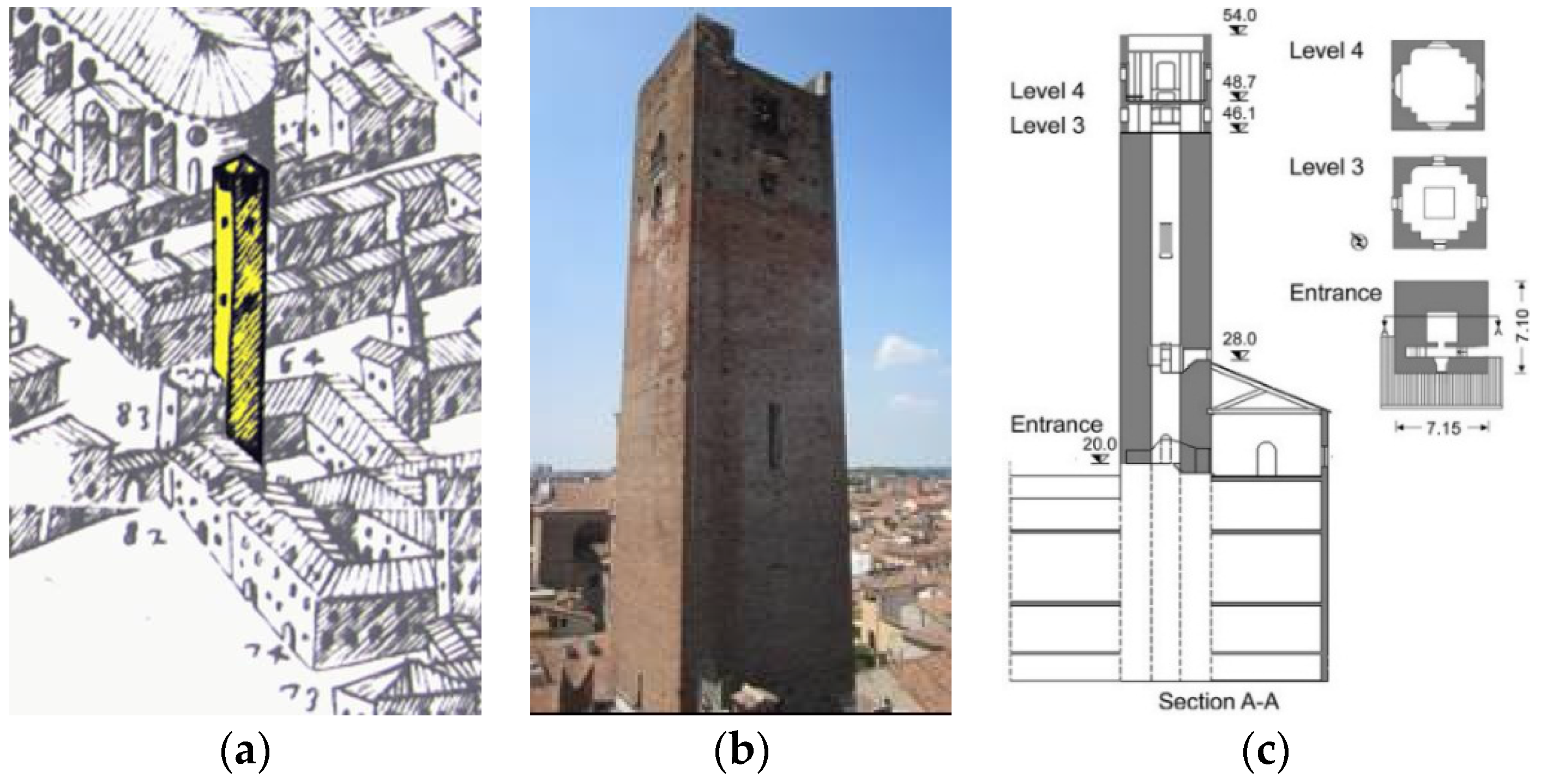
After the earthquake, an extensive research program was carried out to assess the structural condition of the tallest historic tower in Mantua: the Gabbia tower [4,5]. The tower (Figure 1), about 54.0 m high, is a symbol of cultural heritage in Mantua so that the fall of masonry pieces from its upper part, reported during the earthquake occurred on 29 May 2012 [1], provided strong motivations for deeply investigating the structural condition of the building. The post-earthquake survey, described in [6], included: (a) historic and documentary research; (b) an on-site survey and visual inspection of the load-bearing walls and structural discontinuities; (c) non-destructive and minor-destructive tests of materials on site; and (d) dynamic tests in operational conditions.

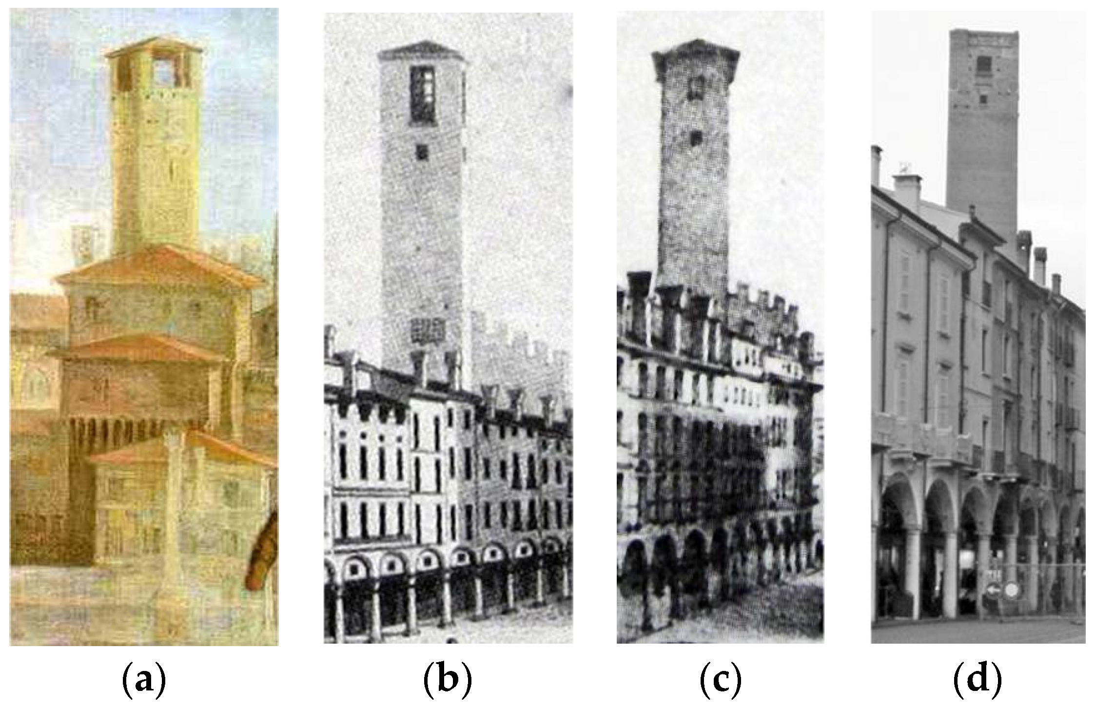
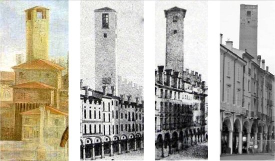
As shown in Figure 2, the available historic pictures indicate modifications and successive additions at the top of the tower. Visual inspection [6] of the upper load-bearing walls revealed traces of past structures on all fronts, and ineffective links between the added parts and extended masonry decay. In addition, one local mode—involving the top of the building—was clearly detected in the dynamic tests [6]; the presence of such a local mode highlights the remarkable structural effects of the change in the morphology and quality of masonry observed on top of the tower and, along with the poor structural arrangement of the upper region, suggests the need for repair interventions to be carried out.

While waiting for the retrofit design and funding, a dynamic monitoring system (consisting of three highly-sensitive accelerometers and one temperature sensor) was installed in the tower [7] for structural health monitoring (SHM) purposes. The continuous dynamic monitoring was mainly aimed at: (a) evaluating the response of the tower to the expected sequence of far-field seismic events; (b) assessing the impact of the environmental (i.e., temperature) effects on the natural frequencies of the building [7,8,9,10,11,12,13]; and (c) detecting the occurrence of any abnormal change or anomaly in the structural behavior. Further potential objectives are providing the retrofit design with additional information and evaluating the effects of the future strengthening.

Approximately six months after the beginning of the continuous monitoring, the tower was subjected to a far-field earthquake [14] and the maximum measured acceleration exceeded about 50 times the highest response that was observed under normal ambient excitation; hence, the monitoring project provided with a challenging opportunity to identify the occurrence of seismic-induced damage under a changing environment.

After a brief description of the investigated tower and the post-earthquake survey, the paper presents the results of the first 15 months of dynamic monitoring and full details are given on the following main tasks: (1) installation of the continuous dynamic monitoring system with remote control and data transmission via the Internet; (2) development of efficient tools [15] to process the raw data regularly received and to automatically identify the modal parameters [16]; (3) tracking the evolution in time of natural frequencies and modeling the temperature effects on those features; and (4) identification of structural performance anomalies.

2. Description of the Gabbia Tower (Mantua, Italy) and On-Site Tests

The Gabbia tower [4,5], about 54.0 m high, is the tallest tower in Mantua and recent research dates the end of its construction to 1227. The building (Figure 1) was part of the defensive system of the Bonacolsi family, governing Mantua in the 13th century. As shown in Figure 1, the tower is, nowadays, part of an important palace, whose load-bearing walls seem not to be effectively connected to the tower walls; nevertheless, the several vaults and floors of the palace are directly supported by the tower.

The tower has a nearly square plan and the load-bearing walls, built in solid brick masonry, are about 2.4 m thick except for the upper levels, where the section decreases to about 0.7 m and a two level lodge is hosted (Figure 1c). Over the past centuries, the lodge was used for communication and military purposes and was accessible through a wooden staircase. The staircase has not been practicable since the 1990s and the access to the inside of the tower was re-established only in October 2012, when provisional scaffoldings and a light wooden roof were installed to allow the visual inspection of the inner load-bearing walls.

After the seismic sequence of May–June 2012 [1], an on-site survey of all outer fronts of the tower was performed using a movable platform and visual inspection highlighted two different structural conditions for the tower:

(a)

in the main part of the building, until about 46.0 m from the ground level, no evident structural damage was observed and the materials appeared mainly affected by superficial decay;

(b)

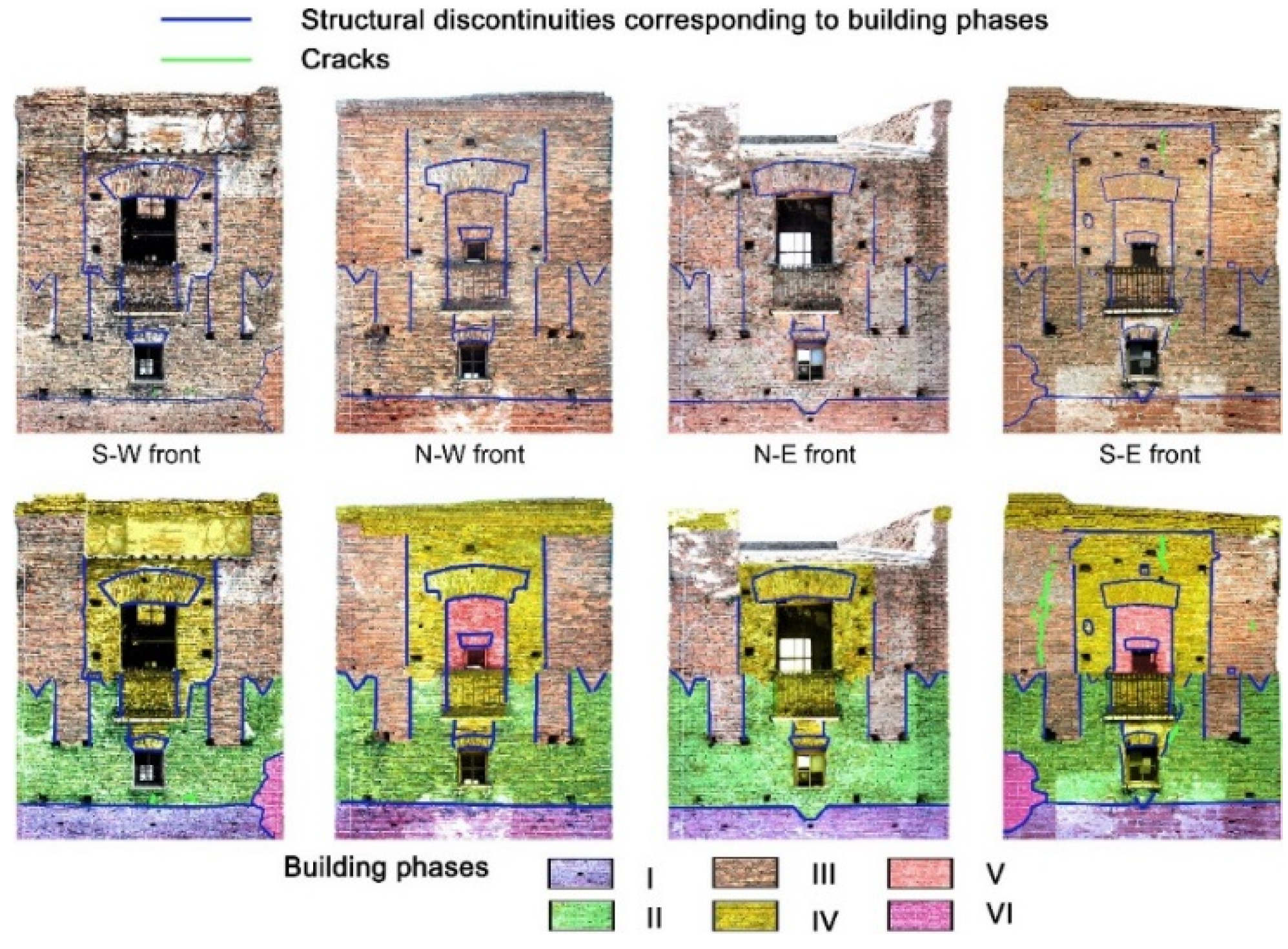
at about 8.0 m from the top, the brick surface workmanship exhibits a clear change [6] and the upper portion of the tower is characterized by passing-through structural discontinuities on all fronts (Figure 3), corresponding to the successive building phases and modifications (Figure 2), as well as by extensive masonry decay. Moreover, the stratigraphic sequencing of masonry (i.e., the well-known methodology coming from archaeology and aimed at obtaining the relative dating of different parts or stratigraphic units) allowed the recognition of at least six main building phases of the upper region of the tower, as shown in Figure 3.

It is further noticed that all fronts of the tower includes merlon-shaped discontinuities (building phase II in Figure 3), recalling the defensive purpose of the original medieval architecture.

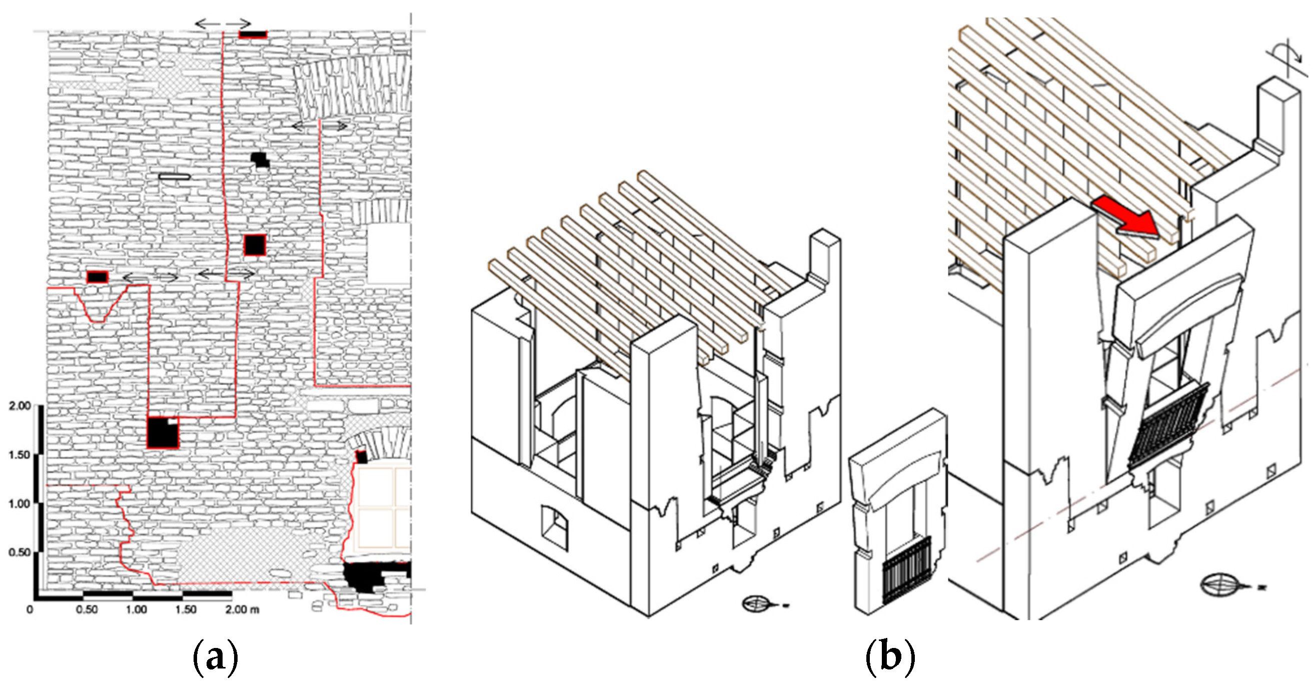
The mapping of the structural discontinuities (Figure 3) determined concerns on the seismic behavior of the upper part of the tower: due to the lack of effective mechanical links between the added parts, some weakly restrained portions could overturn under the earthquake actions. Based on this investigation, a first evaluation of out-of-plane seismic behavior for each identified masonry portion not effectively linked was carried out, as shown in Figure 4, and safety factors of about 1.15–1.20 were estimated for the earthquake occurred on May–June 2012 [1]. Furthermore, low intensity seismic actions, such as after-shocks or far-field earthquakes, could worsen the weak connection between the different elements by decreasing the adhesion and accentuating the boundaries.

Further evidence of the poor compactness of the materials in the upper region of the structure was attained by performing pulse sonic tests at different levels of the tower: the average value of sonic velocity measured at the upper levels is 600 m/s, whereas the sonic velocity values range between 1100 m/s and 1600 m/s until a height of 46.0 m.

As previously pointed out, a wooden roof (Figure 5a) was installed in the upper part of the tower when the inner access was re-established through metallic scaffoldings (Figure 5b). The roof, although very light, rests directly on the weakest region of the structure and is slightly inclined (Figure 5a). Hence, the roof slope and the redundant connection with the masonry walls, as well as thermal effects, might cause non-negligible thrusts on the crowning walls, which are very vulnerable due to the presence of several discontinuities, the lack of connection of the different additions (Figure 4), and the extensive decay.

3. Preliminary Operational Modal Tests and Dynamic Characteristics of the Tower

Two series of ambient vibration tests (AVTs) were conducted on the tower. The first test was carried out between 31/07/2012 and 02/08/2012 [6] with the objectives of evaluating: (a) the dynamic characteristics of the tower; (b) the possible effects of the poor state of preservation of the upper region on the global behavior; and (c) the impact of temperature changes on the natural frequencies. The second test, preparatory to the continuous dynamic monitoring, was performed on 27/11/2012 with the two-fold objective of evaluating the possible effects of added wooden roof and scaffoldings (Figure 5) and providing reference values of the modal parameters for the subsequent monitoring.

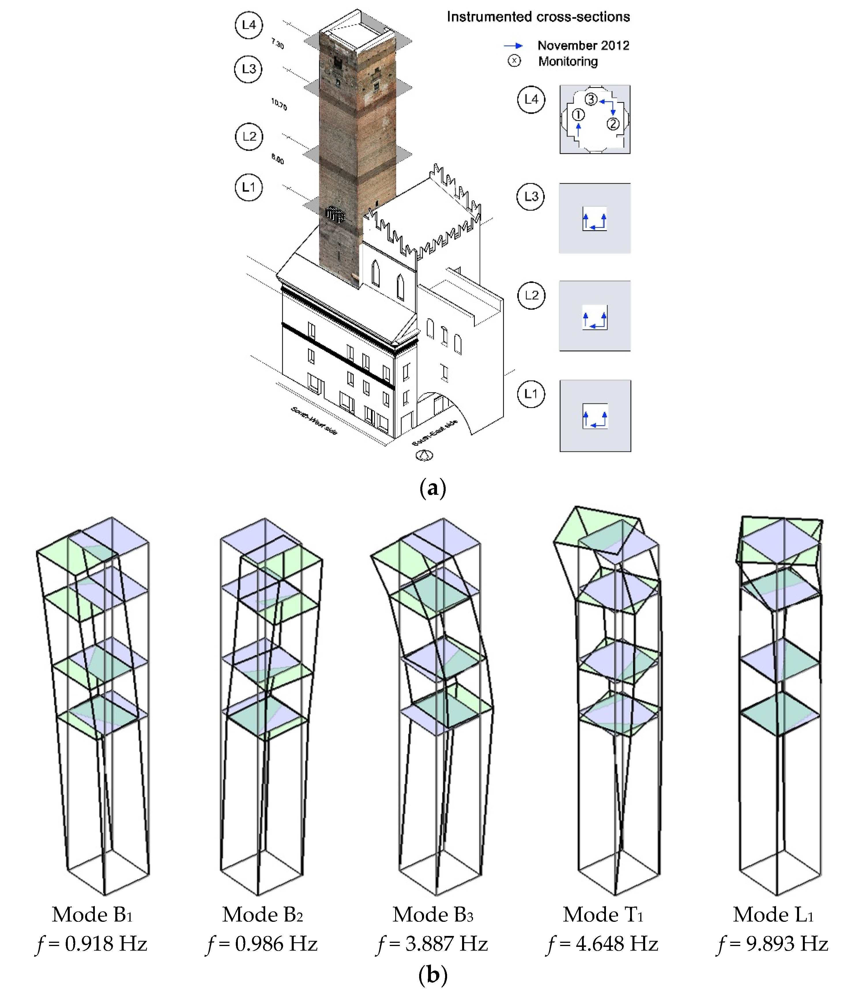
During both tests high-sensitivity accelerometers (WR model 731A, 10 V/g sensitivity and 0.5 g peak acceleration, Wilcoxon Research, Germantown, MD, USA) were used to measure the dynamic response of the tower in 12 points, belonging to four pre-selected cross-sections along the height of the building (Figure 6a). Since access to the inner walls of the tower was not available during the first survey, the accelerometerswere mounted on the outer walls making use of the same movable platform employed for visual inspection. During the second test, performed after the installation of wooden roof and provisional scaffoldings inside the tower (Figure 5), inner mounting of the accelerometers was preferred (Figure 6a).

The modal identification was performed considering time windows of 3600 s and applying the data-driven stochastic subspace Identification algorithm (SSI-Data) [17,18] available in the commercial software ARTeMIS Extractor [19] (Release 5.3, SVS, Aalborg, Denmark, 2012).

Since the second test was aimed at estimating the modal parameters used as reference values in the continuous dynamic monitoring, only the results of this test will be presented herein.

The application of the SSI-Data method to the datasets collected in the test of November 2012 (about two hours of acceleration data recorded with an outdoor temperature of 10 °C–11 °C) allowed the identification of five vibration modes in the frequency range of 0–10 Hz. Figure 6b summarizes the identified dynamic characteristics of the tower and allows the following comments:

(a)

two closely-spaced modes (B₁ and B₂) were identified in the frequency range of 0.90–1.00 Hz and are associated to dominant bending in the two main planes of the tower, respectively. The modal deflections of first mode (B₁) involve bending in the N-E/S-W direction, whereas the second mode (B₂) is dominant bending in the orthogonal N-W/S-E direction;

(b)

the third mode (B₃) is dominant bending in the N-E/S-W direction with slight components also in the orthogonal direction;

(c)

the fourth mode (T₁) is characterized by dominant torsion until the height of 46.0 m and coupled torsion-bending of the top level. The local behavior of the upper region of the tower alters what would otherwise be classified as a pure torsion and was not observed in the previous dynamic test so that it can be conceivably associated to both the poor structural condition of the upper level and the effect exerted by the wooden roof, directly resting on the weakest region of the tower; and

(d)

a local mode (L₁) was identified at 9.89 Hz and involved torsion of the top levels of the tower. The presence of a local mode provides further evidence of the structural change in the masonry quality and morphology highlighted in the upper part of the building by the visual inspection.

It is worth mentioning that the fundamental frequencies of about 1 Hz exactly fall in the range of dominant frequencies characterizing the earthquakes recorded in Mantua on May 2012 and, more generally, the earthquakes expected in the Mantua region conceivably explain the fall of small masonry pieces from the upper part of the building, reported during the earthquake of 29 May 2012.

4. Continuous Dynamic Monitoring of the Gabbia Tower

A few weeks after the execution of the preliminary AVTs, a simple dynamic monitoring system was installed in the tower. The monitoring system is composed by: (a) three piezoelectric accelerometers (WR model 731A, 10 V/g sensitivity and ±0.50 g peak, Wilcoxon Research, Germantown, MD, USA), mounted on the cross-section at the crowning level of the tower (Figure 6a); (b) one temperature sensor (TRAFAG, Legnano, Italy), installed on the S-W front and measuring the outdoor wall temperature; (c) one four-channel data acquisition system (24-bit resolution, 102 dB dynamic range, and anti-aliasing filters) (National Instruments, Austin, TX, USA); and (d) one industrial PC on site, for the system management and data storage. A binary file, containing three acceleration time series and the temperature data, is created every hour, stored in the local PC and transmitted to Politecnico di Milano for being processed.

The continuous dynamic monitoring system has been active since 17/12/2012. The data files received from the monitoring system are managed by a LabVIEW toolkit [15] (National Instruments, Austin, TX, USA), including the (on-line or off-line) execution of the following tasks:

(1)

creation of a database, with the original data in compact format, for later developments;

(2)

data pre-processing, i.e., de-trending, automatic recognition, and extraction of possible seismic events, and creation of one dataset per hour;

(3)

statistical analysis of data. This task includes also the evaluation of the hourly-averaged temperature and the computation of the root mean square (RMS) accelerations associated to each 1-h dataset; and

(4)

low-pass filtering and decimation of the each dataset and creation of a second database in ASCII format, with essential data records, to be used in the modal identification phase. In more details, the recorded accelerations were low-pass filtered—using a classic seventh-order Butterworth filter with a cut-off frequency of 20 Hz—and decimated five times, reducing the sampling frequency from 200 Hz to 40 Hz.

4.1. Automatic System Identification

As in the preliminary tests, the identification of modal parameters was carried out considering time windows of 3600 s, in order to largely comply with the widely-agreed recommendation [20] of using a minimum duration of the acquired time window (which should be 1000–2000 times the fundamental period of the structure) to obtain accurate estimates from output-only data. In fact, output-only methods assume that the (un-measured) excitation input is a zero mean Gaussian white noise and this assumption is as closely verified as the length of the (measured outputs) time window is longer.

The modal parameters of the building were estimated from the measured signals using an automatic procedure [16], based on the covariance-driven stochastic subspace Identification (SSI-Cov) method [17,18].

In the SSI-Cov algorithm [17,18], the covariance matrices of the m measured outputs are computed, for positive time lags varying from Δt to (2i−1)Δt, to fill a (mi × mi) block Toeplitz matrix, that is decomposed to estimate stochastic subspace models—i.e., matrices A, C—of increasing order n. Once matrices A, C of different order n are obtained, n/2 sets of modal parameters are extracted from a model of order n: natural frequencies and damping ratios are calculated from the eigenvalues of A, whereas the mode shapes are evaluated from the product of C and the eigenvectors of A.

In the automated procedure [16], each stabilization diagram (where the modes associated to increasing model order are plotted together) was “cleaned” from certainly spurious modes firstly by detecting system poles with non-physical characteristics through a damping ratio check, and subsequently by excluding the poles whose mode shapes exhibit a high modal complexity [21]. Similar modes in the cleaned stabilization diagram are grouped together based on the sensitivity of frequency and mode shape change to the increase of the model order. Finally, the identified modal parameters are compared to the reference results, available from the preliminary test.

In the present application, the time lag parameter i was set equal to 70 and the data was fitted using stochastic subspace models of order n varying between 30 and 120.

4.2. Temperature Effects on Natural Frequencies: Dynamic Regression and ARX Models

As measuring the dynamic response using few accelerometers provides information mainly on the natural frequencies, these parameters have to be necessarily used as features sensitive to abnormal structural changes and damage. However, the natural frequencies of masonry towers are also affected by factors other than damage, such as temperature [9,10,11,12,13]. It should be noticed that, as reported in [9], the humidity might also affect the modal frequencies of masonry towers, with the increase of water absorption (in the rainy season) inducing a temporary decrease of natural frequencies; on the other hand, no appreciable effects of air humidity on natural frequencies have been detected in [11,13].

Since masonry towers are generally subjected to low levels of ambient excitation, it has to be expected that the modal frequencies are mainly affected by changing temperature. Hence, the correlation between natural frequencies and temperature needs to be investigated for early detection of structural anomalies: once the normal response of a structural system to changes in its environmental conditions has been explored and can be filtered out to normalize the response data, any further changes in the sensitive features should rely to changes of the structural condition.

In order to characterize the effects of temperature on the natural frequencies, dynamic regression (DR) models were established for each identified frequency. DR models [22] assume that the value y_k of the dependent variable (i.e., natural frequency) at time instant k is influenced by the values of the model input (i.e., temperature) at current time k, as well as at (p−1) previous time instants:

$$y_k=b_1\times x_k+b_2\times x_{k-1}+\dots +b_p\times x_{k-\left(p-1\right)}+{\mathsf{\epsilon }}_k$$

(1)

The linear model (1) can be expressed in matrix form as:

y = Xb + ε

(2)

where y℘Rⁿ is the vector containing n observations y_k of the dependent variable, b℘R^p is the vector formed by the p parameters weighting the contribution of the input, ε℘Rⁿ is the vector of the random errors and X℘R^n×p is the matrix appropriately gathering the values of the input.

Models (1) and (2) can be further generalized so that predictions are computed which also consider previous values of the dependent variables. Among the dynamic methods described in the system identification literature (see e.g., [23]), the Auto-Regressive models with eXogenous input (ARX) are probably the most widely used. ARX models [23] consist of an auto-regressive output and an exogenous input part and can be expressed in the following form:

$$y_k+a_1\times y_{k-1}+\dots +a_{n_a}\times y_{k-n_a}=b_1\times x_{k-n_k}+b_2\times x_{k-n_k-1}+\dots +b_{n_b}\times x_{k-n_b+1}+{\mathsf{\epsilon }}_k$$

(3)

Of course, the linear model (3) can be expressed in the matrix form (2). It should be noted that in Equation (3) only one input (e.g., temperature) and one output (e.g., natural frequency) were considered. Equation (3) can be easily generalized to the case of multiple inputs by replacing y_k and x_k with corresponding row and column vectors, respectively. ARX models are characterized by three model orders: the auto-regressive order n_a (corresponding to the number of the considered past measures of the dependent variable), the exogenous order n_b (corresponding to the number of previous model inputs taken into account), and the time delay between input and output n_k. Orders n_a and n_b determine the number of model parameters.

It is worth mentioning that: (a) in the framework of a dynamic monitoring project, different input candidates might be considered in the dynamic regression model (1) and (2), such as temperature, humidity, wind speed, traffic loads on bridges, etc. (see e.g., [24,25,26]); (b) in order to properly describe the influence of changing environmental conditions, the data used to estimate the parameters of the regression models should be collected over a significant period of time, denoted as the training period (or reference period), and including a statistically representative sample of temperature conditions.

Once DR or ARX models have been established for the identified frequencies, the impact of changing environment on each modal frequency should be eliminated (or at least minimized) by defining the following quantities:

(a)

The residual error vectors ε_i = y_i − X_ib_i (i = 1, 2, …, M where M is the number of automatically identified modal frequencies); and

(b)

The cleaned observation vectors y_i* = 1 μ_i + ε_i (i = 1, 2, …, M where 1 is the unit vector and μ_i is the mean value of the identified i-th frequency data in the reference period).

Hence, both the residual error and the cleaned observation vectors might be used to identify the occurrence of abnormal structural changes or damages not observed during the training period.

5. Monitoring Results and Data Analysis

This section presents the main results of the continuous dynamic monitoring for a period of 15 months, from 17/12/2012 to 17/03/2014. During the examined monitoring period, more than 10000 1-h datasets were collected, with the ambient excitation being mainly provided by micro-tremors and wind, and automated modal identification has been performed.

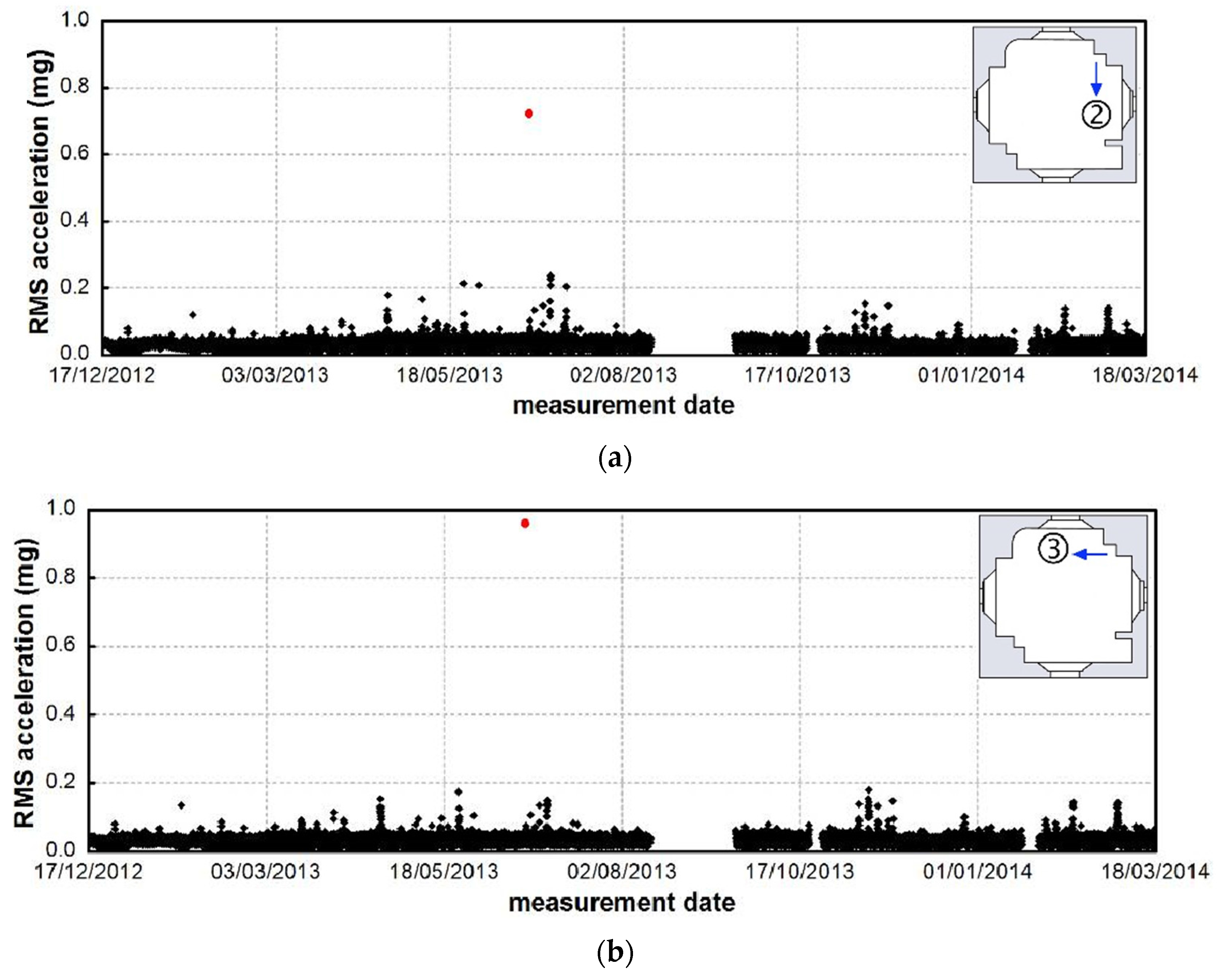
Figure 7 shows the RMS value of the acceleration measured at points 2 and 3 (Figure 6a), computed considering time windows of 1 h. The inspection of Figure 7 highlights that: (a) the ambient excitation is generally very low and the RMS acceleration does not exceed 0.05–0.06 mg (with the corresponding peak accelerations being lower than 0.4 mg); (b) windy days are easily identified through “alignments” of RMS acceleration points in the range 0.06–0.20 mg. Furthermore, the information provided by the weather station in Mantua and the Italian Institute of Geophysics and Volcanology (INGV) allowed the classification of the isolated points exceeding the amplitude of 0.06 mg as generally associated to far-field seismic events or large micro-tremors.

It should be noticed that, until June 2013, the tower’s response to different far-field earthquakes was recorded by the monitoring system. The strongest seismic event—corresponding to the earthquake (5.2 Richter magnitude) that occurred in the Garfagnana region (Tuscany) on 21/06/2013 [14] and strongly felt in many regions of Northern Italy—is marked in red in Figure 7 and was characterized by a measured peak acceleration of about 20 mg, exceeding about 40–50 times the highest amplitude of normally observed ambient vibrations.

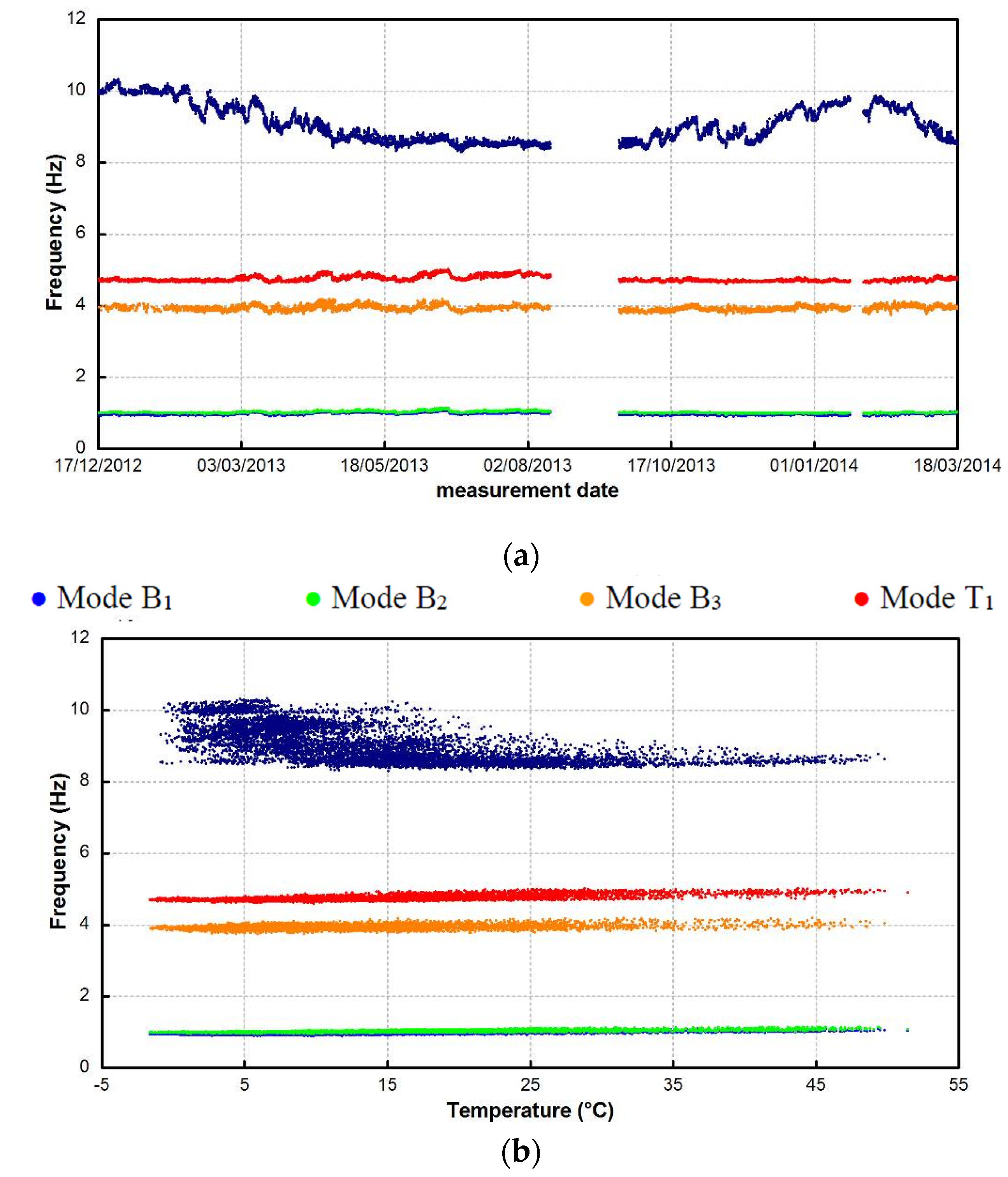
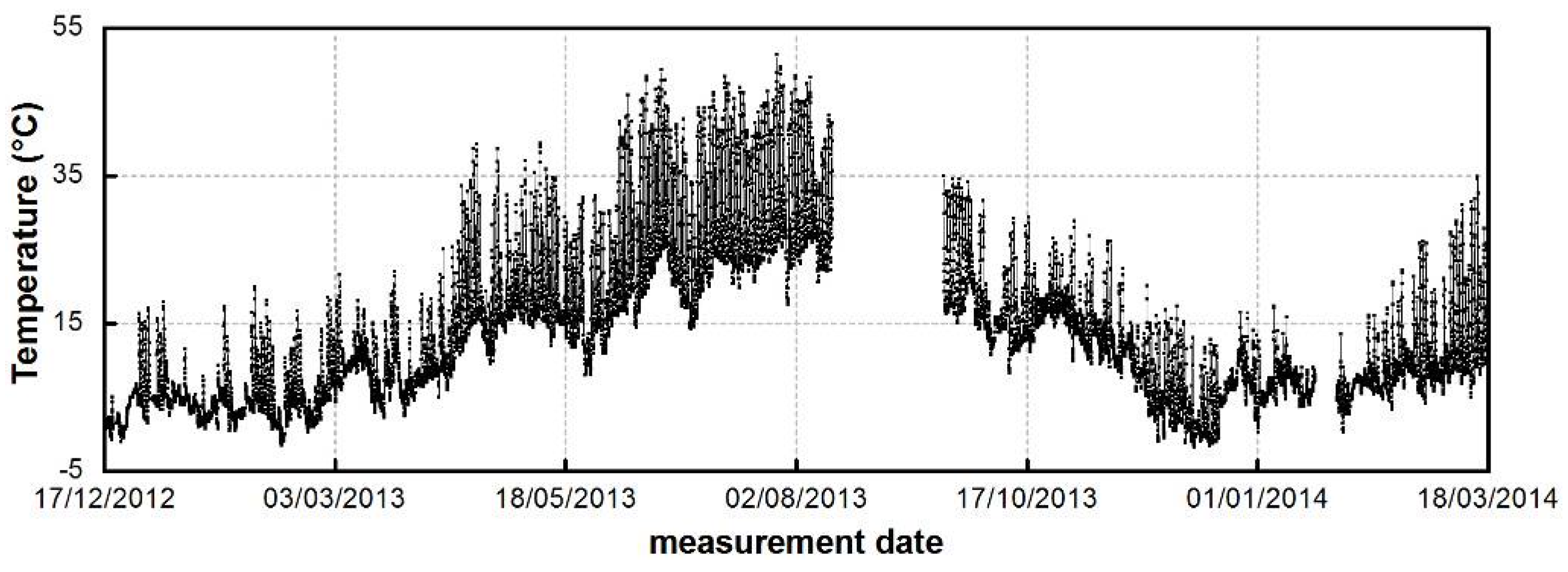
Figure 8 shows the evolution in time of the outdoor temperature (S-W front) and reveals yearly variations, ranging between −2 °C and 45 °C, and daily fluctuations of about 30 °C in sunny days. The corresponding variations of the modal frequencies vs. time (Figure 9a) and vs. temperature (Figure 9b) indicate that the natural frequencies of the global modes (B₁–B₃ and T₁, Figure 6b) are related to the temperature. More specifically, Figure 9b shows that the frequency of global modes tends to increase with increased temperature. This behavior, observed also in other studies of masonry towers [9,10,11,12,13], is conceivably related to the materials thermal expansion that, in turn, gives rise to the closure of minor masonry discontinuities, superficial cracks, and mortar gaps. Hence, the “compacting” of the materials induces a temporary increase of stiffness and modal frequencies, as well.

The statistics of the natural frequencies identified from 17/12/2012 to 17/03/2014 are summarized in

Table 1. Statistics of the natural frequencies identified (SSI-Cov) from 17/12/2012 to 17/03/2014.

Mode	fmean (Hz)	σf (Hz)	fmin (Hz)	fmax (Hz)
1 (B1)	0.977	0.035	0.903	1.102
2 (B2)	1.017	0.028	0.960	1.148
3 (B3)	3.935	0.069	3.742	4.194
4 (T1)	4.741	0.073	4.600	5.010
5 (L1)	9.062	0.511	8.332	10.327

B = bending mode; T = torsion mode; L = local mode.

. This table includes the mean value (f_mean), the standard deviation (σ_f), and the extreme values (f_min, f_max) of each modal frequency. It should be noted that standard deviations are larger than 0.03 Hz for all global modes and especially significant for the local mode. Indeed, the frequency evolution of mode L₁ looks very different from the others (Figure 9) and characterized by remarkable variations, as the natural frequency ranges between 8.33 Hz and 10.33 Hz over the examined time period.

A close inspection of the frequency tracking of mode L₁ allows the recognition of three different phases of the frequency evolution in time: (a) in a first phase (between 17/12/2012 and 14/08/2013) the modal frequency clearly decreases in time, from an initial value of about 10.0 Hz to a final value of about 8.5 Hz; (b) after the summer period (from 19/09/2013 to 19/01/2014) the frequency increases again, even if the new maximum values do not reach those identified one year before in similar environmental conditions; and (c) finally, the natural frequency decreases again from 02/02/2014 to the end of the monitoring period. Furthermore, each of those three phases is characterized by the presence of some discontinuities (drops or increases), which define the general trend of the frequency tracking.

For example, considering the first time period, three drops can be detected at the beginning of February 2013, at mid-March 2013, and at mid-April 2013 [7]. These drops divide the examined time span in four parts, which can be easily identified in the temperature-frequency plot of Figure 10. This figure highlights that the populations of temperature-frequency points, corresponding to the four different periods, exhibiting similar slope of the best fit line, whereas the average frequency value significantly decreases. The subsequent time periods are characterized by similar trends, with the frequency increasing and decreasing, respectively.

It should be noted that the changes exhibited by the frequency of the local mode, illustrated in Figure 9 and Figure 10, can hardly be explained by moisture. In fact, the figures show that the natural frequency of the local mode tends to decrease as: (a) the average daily temperature increases and (b) the temperature daily range includes higher temperatures. On the contrary, it has to be expected [9] that the modal frequency decreases with increased water absorption (i.e., the moisture inside the walls) at the beginning of the raining season and not at the beginning and during the hot seasons, as it happens in the present case (Figure 9a and Figure 10).

The observed behavior suggests the progress of a possible damage mechanism, conceivably related to the effect exerted by the wooden roof with increased temperature, and confirms the poor structural condition of the upper part of the tower, as well as the need of preservation actions. This conclusion seems to be confirmed also by the frequency loss detected after one year of monitoring, with the natural frequency of the local mode being unable to reach the maximum values identified one year before in similar environmental conditions.

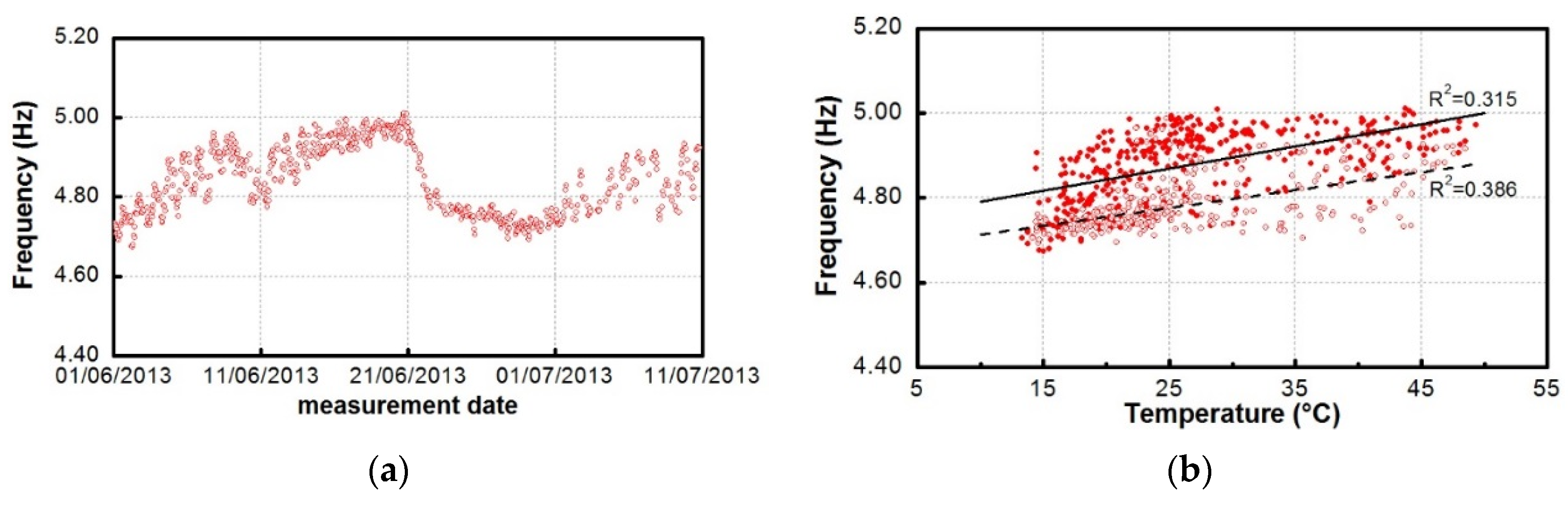
As previously pointed out, the earthquake occurring in the Garfagnana region on 21/06/2013 [14] determined accelerations on top of the Gabbia tower that were significantly higher (Figure 7) than the usual ambient vibration responses.

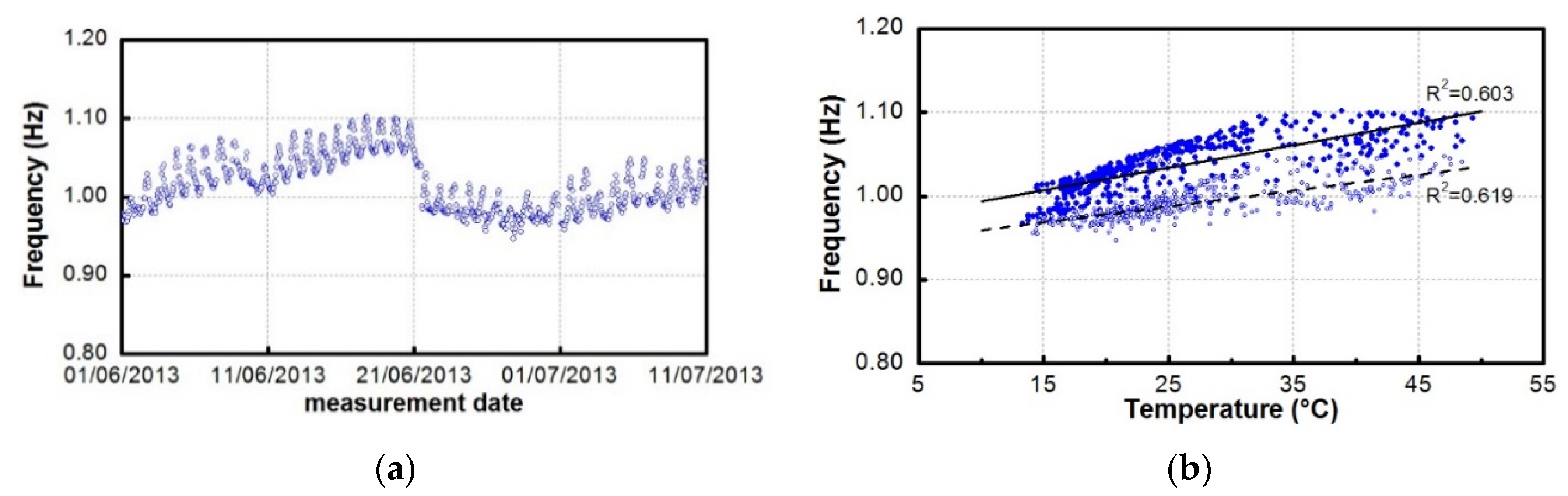
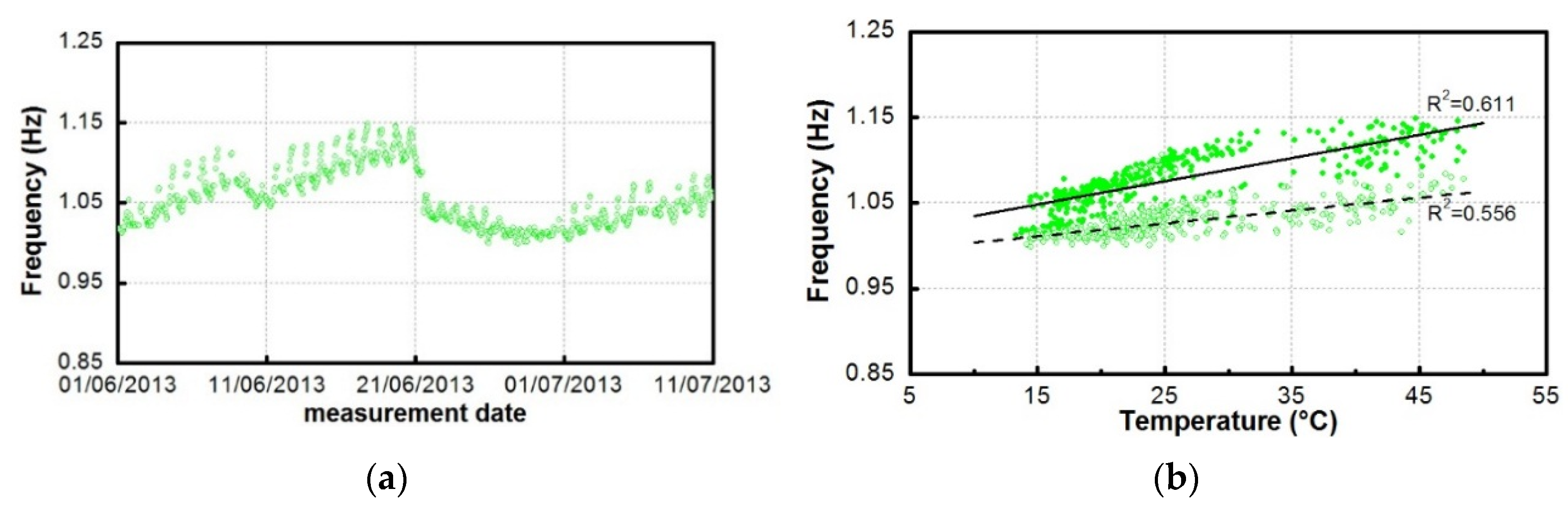
Zooming in the time evolution of the natural frequencies of modes B₁, B₂, and T₁—considering three weeks before and three weeks after the earthquake—is shown in Figure 11a, Figure 12a, and Figure 13a; the figures show a clear decrease of all modal frequencies on 21/06/2013, corresponding to the occurrence of the seismic event. Furthermore, the temperature-frequency relationships (Figure 11b, Figure 12b, and Figure 13b) highlight that the regression lines of all modes exhibited clear variations after the earthquake, with the temperature range being almost unchanged. It is worth mentioning that this trend is confirmed by:

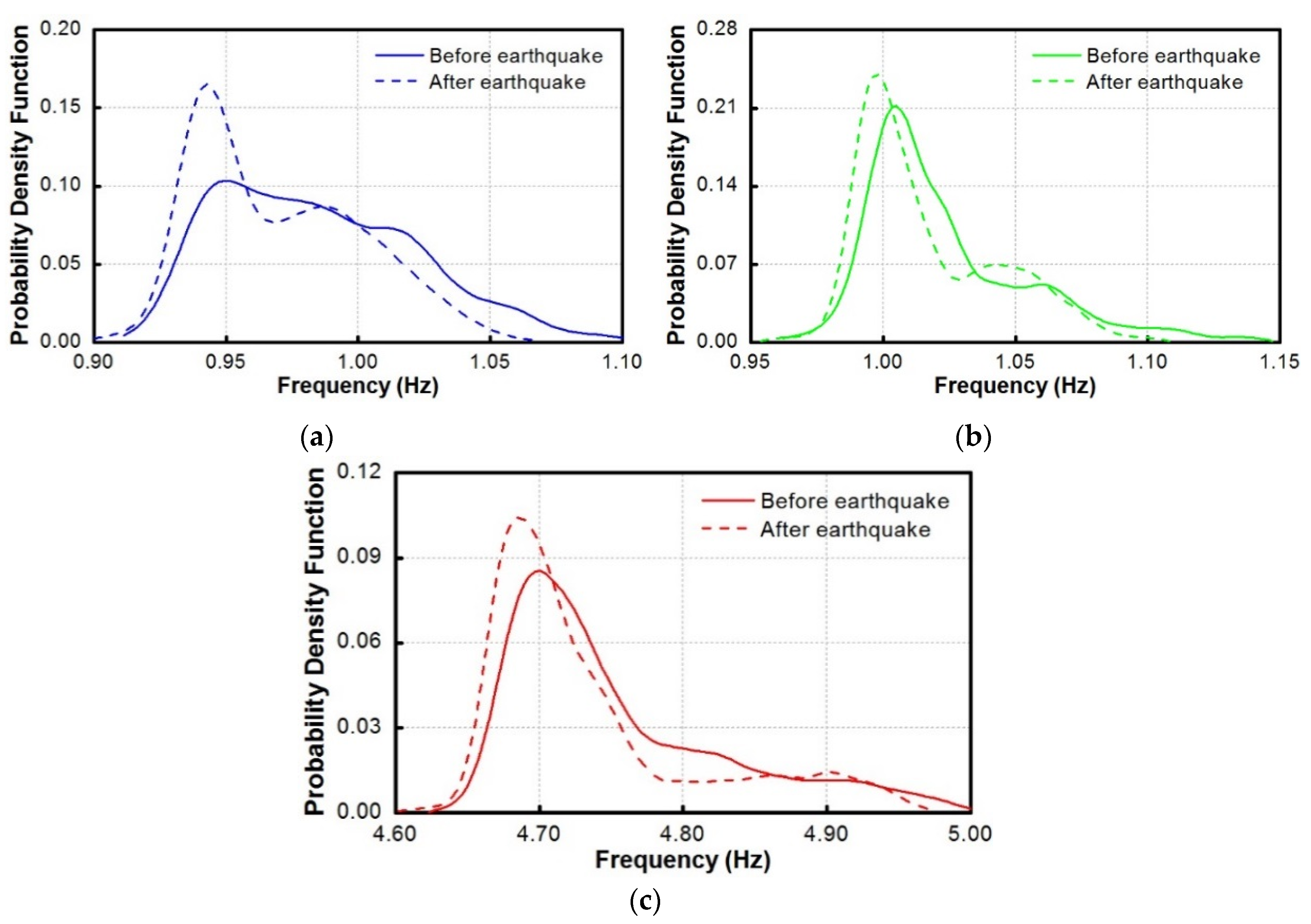
(a)

Estimating the distribution of the modal frequencies before and after the seismic event. The estimate—shown in Figure 14 for modes B₁, B₂, and T₁—is based on a normal kernel function, which was evaluated at 100 equally-spaced frequency bins covering the range of variation of each identified frequency. The probability density functions presented in Figure 14 refer to the six months before (from 17/12/2012 to 20/06/2013, solid line) and the six months after the earthquake (dashed line). The inspection of the plots reveals that the frequency distributions change after the seismic event and indicates that the identified frequencies slightly shift towards lower values after the earthquake;

(b)

The general decrease of the statistics of the natural frequencies (mean value, standard deviation, extreme values) summarized in

Table 2. Statistics of the modal frequencies identified before and after the seismic event of 21/06/2013.

Mode	fmean (Hz)		σf (Hz)		fmin (Hz)		fmax (Hz)
	Before	After	Before	After	Before	After	Before	After
1 (B1)	0.985	0.968	0.038	0.031	0.910	0.897	1.102	1.070
2 (B2)	1.024	1.012	0.032	0.025	0.961	0.953	1.148	1.110
3 (B3)	3.941	3.929	0.075	0.063	3.758	3.742	4.194	4.137
4 (T1)	4.754	4.727	0.077	0.066	4.621	4.600	5.010	4.982
5 (L1)	9.222	8.937	0.554	0.433	8.385	8.332	10.327	9.862

B = bending mode; T = torsion mode; L = local mode.

and, again, demonstrating the occurrence of abnormal structural changes induced by the seismic event.

Based on the previous evidence, it can be stated that the limited number of accelerometers and temperature sensors installed in the tower and the automatic system identification allowed for the assessment of the effects of changing temperature on modal frequencies and to detect the occurrence of abnormal structural behavior under changing environment.

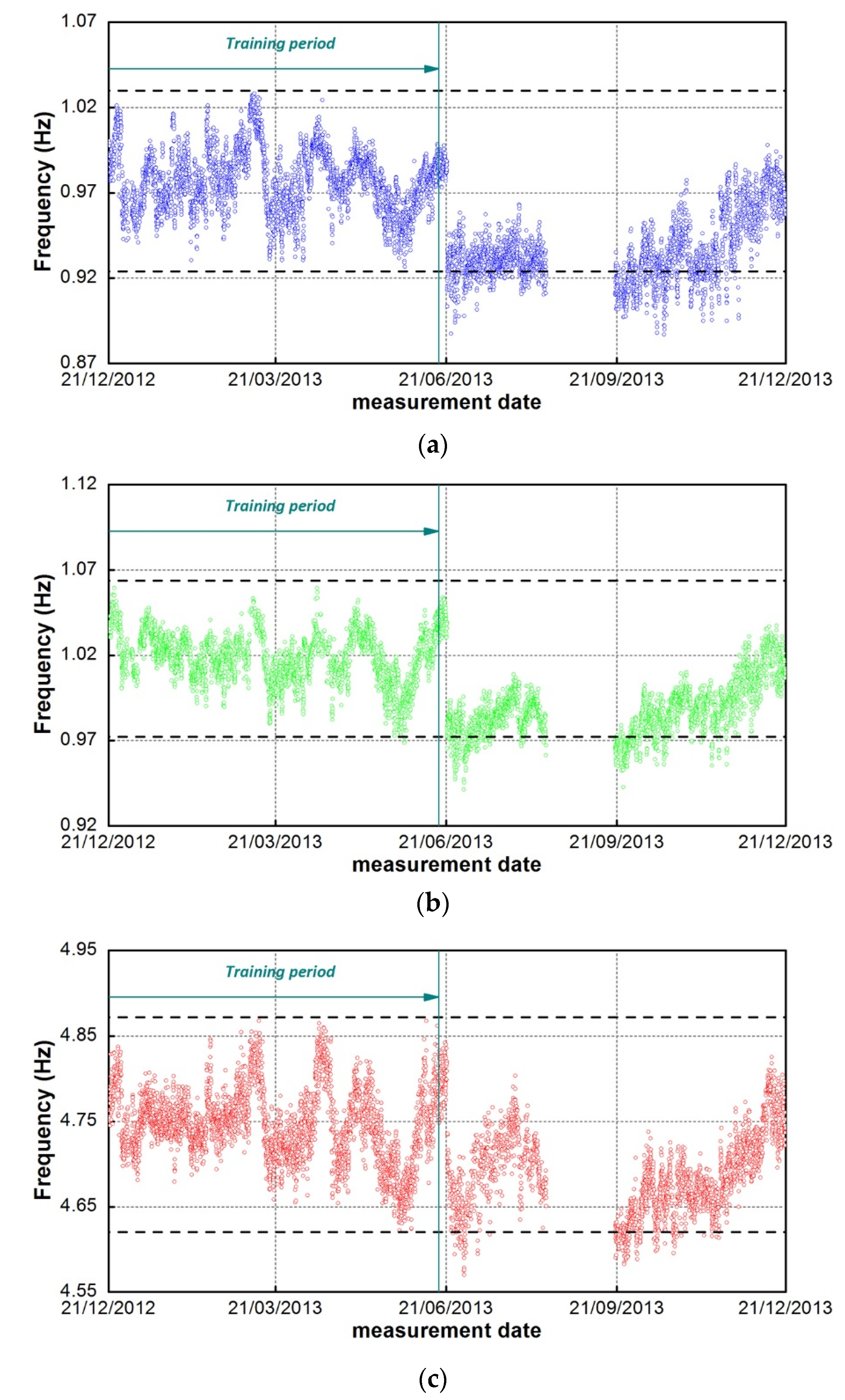
5.1. Damage Detection under Changing Environment

As stated in Section 4.2, the temperature effects on the natural frequency of each global mode have been described by means of DR models, with the outdoor temperature measured on the S-W front as its only input. Based on the classic loss function (LF) and the final prediction error (FPE) criteria [23], regression models depending on the current and 13 previous hourly-averaged values (p – 1 = 13) of the external temperature have been established.

As the main goal was to mitigate the environmental effects in order to verify if the structural changes induced by the earthquake of 21/06/2013 are still detected, the models were trained over the six months preceding that seismic event (from 17/12/2012 to 16/06/2013), where the process is supposed to be in control. The dynamic regression models were subsequently used to predict the natural frequencies after the training period and to detect the changes in the structural behavior. The relevant results—in terms of cleaned natural frequencies of modes B₁, B₂ and T₁—are presented in Figure 15 with the confidence limits at plus and minus three times the standard deviation of the frequency estimated obtained over the training period.

It is worth noting that the representation in Figure 15 is centered on the earthquake date (21/06/2013), in order to better highlight the different trends before and after the seismic event. The inspection of the cleaned modal frequencies (Figure 15) allows the following comments:

(a)

the natural frequencies still exhibit some correlation, meaning that they are still affected by common factors;

(b)

before the seismic events, each frequency oscillates around its mean value and stays within the confidence interval; and

(c)

a sudden drop is detected corresponding to the earthquake, along with a clear variation of the previous trend. More specifically, in the months after 21/06/2013, the mean value of the cleaned natural frequency changes and the confidence interval, estimated in the training period, is exceeded.

Therefore, the correction of the natural frequencies provided by the adopted regression model still indicates that non-reversible structural changes took place after the Garfagnana earthquake.

The DR models, so far discussed, allowed for partially modeling the thermal effects on the natural frequencies of the investigated tower. On one hand, the DR relationship proved to be effective in reproducing the fluctuations of the experimental frequencies due to the daily effect of temperature and in distinguishing the slight damage induced by the Garfagnana earthquake (Figure 15). On the other hand, the model could not as accurately predict the long-term oscillations due to the influence of the average temperature (conceivably combined with the effects of other unobserved factors).

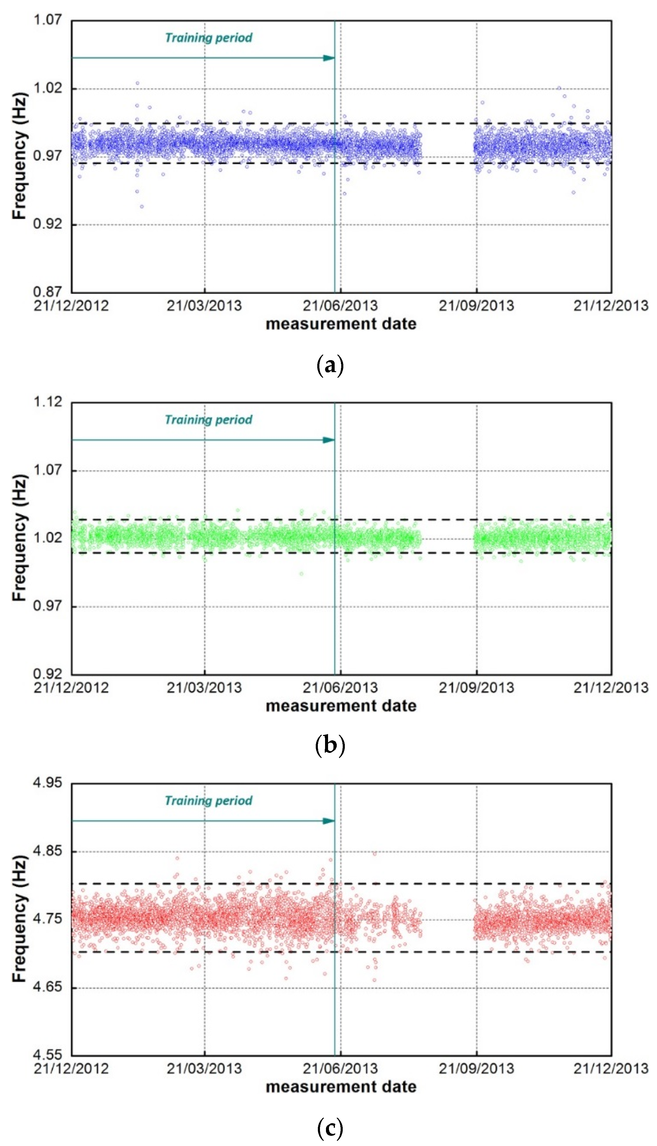
In order to improve the prediction, ARX models have been developed. ARX models assume the value f_k of the natural frequency at time k to be affected by outdoor temperatures at the same time k and at previous time instants, as well as by previous experimental estimates of the input. In particular, the use of past values of the output is expected to indirectly take into account the effects of unmeasured factors that cannot be modeled otherwise (e.g., wind, humidity, etc.) leading, in principle, to more accurate predictions. Since several models can be fitted to the experimental data, depending on the amount of previous time instants considered for the input and the output, a comparative study of the performances has been carried out by using the same LF and FPE criteria [23] adopted for establishing the DR models. Eventually, an ARX240 model has been selected, characterized by n_a = 2 previous estimates of the experimental frequency, n_b = 4 past hourly values of the outdoor temperature, and no delay between input and output (n_k = 0). To calibrate the parameters of the ARX240 model, the same training period used for the DR relationship has been considered, i.e., between 17/12/2012 and 16/06/2013, in order to leave out the structural variation due to the earthquake of 21/06/2013.

The evolution in time of the cleaned natural frequencies of modes B₁, B₂, and T₁ is shown in Figure 16: the non-negligible dispersion of the values and the evident fluctuations characterizing the results of the DR are no longer observed, suggesting that the influence of environmental factors has been completely removed. Unfortunately, none of the depurated frequencies exhibits any sudden variation after the Garfagnana earthquake. A possible explanation for this unexpected behavior could lie in the fact that—as shown in Figure 11a, Figure 12a, and Figure 13a—the frequency drop caused by the seismic event has the same order of magnitude as the fluctuations induced by the temperature effects. Therefore, since the ARX model is able to follow the temperature-induced frequency variations with high accuracy, the sudden drop caused by the seismic event is reproduced as well. This, in turn, jeopardizes the possibility of detecting anomalous occurrences from environment-independent features obtained through ARX models.

6. Conclusions

The paper focuses on the post-earthquake assessment of a historic masonry tower and summarizes the results of visual inspection, ambient vibration tests, and long-term dynamic monitoring of the building.

Visual inspection and the stratigraphic sequencing of the load-bearing walls clearly indicated that the upper part of the tower is characterized by the presence of several discontinuities due to the historic evolution of the building, local lack of connection, and extensive masonry decay. The poor state of preservation of the same region was confirmed by the observed dynamic characteristics, as one local mode, involving the upper part of the tower, was clearly identified from ambient vibration data.

The results of the SHM exercise performed through the continuous dynamic monitoring of the tower at study highlighted that a limited number of accelerometers and temperature sensors installed in the structure are sufficient to provide meaningful information for the preventive conservation and/or SHM of historic towers. More specifically, the following conclusions can be drawn:

• The application of state-of-art tools for automated operational modal analysis allows tracking of natural frequencies;
• The temperature turned out to significantly affect the (daily) variation of the natural frequencies in masonry towers, with the frequencies of global modes increasing with increased temperature;
• Dynamic regression models are suitable to represent the environmental effects on modal frequencies, even when only one (outdoor) temperature sensor is installed in the structure;
• The application of automated operational modal analysis and dynamic regression models turned out to be effective in the identification of seismic-induced structural anomalies under changing environment;
• ARX models are suitable to completely remove the environmental effects from modal frequencies, but exhibit no damage detection skills (i.e., the frequency drops associated to slight abnormal structural changes are not distinguished from similar variations induced by temperature or other unobserved factors);
• The application of automated operational modal analysis highlighted the possible progress of a damage mechanism, involving the upper part of the tower, remarked by the significant fluctuations of the natural frequency of the identified local mode.

As a concluding remark, this full scale experience demonstrates that low-cost dynamic monitoring systems, combined with state-of-art tools for automated operational modal analysis and statistical tools for the minimization of the environmental effects, are effective and sustainable means for the preservation of historic masonry towers.