
Dual-Tree Complex Wavelet Transform and Twin Support Vector Machine for Pathological Brain Detection


Abstract
:
1. Introduction
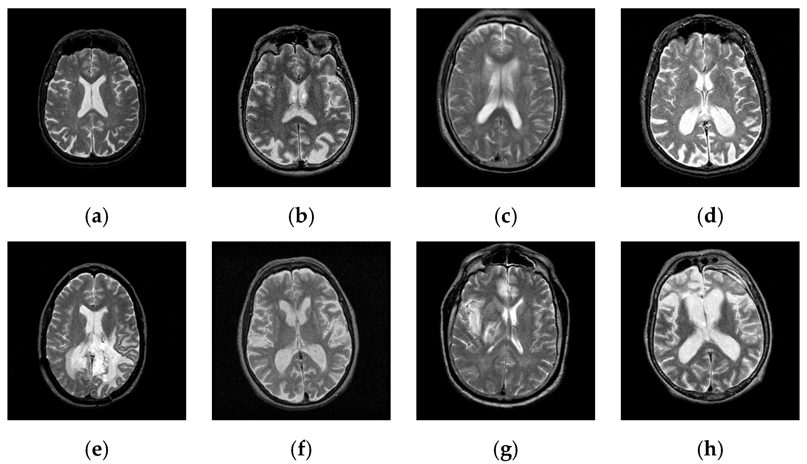
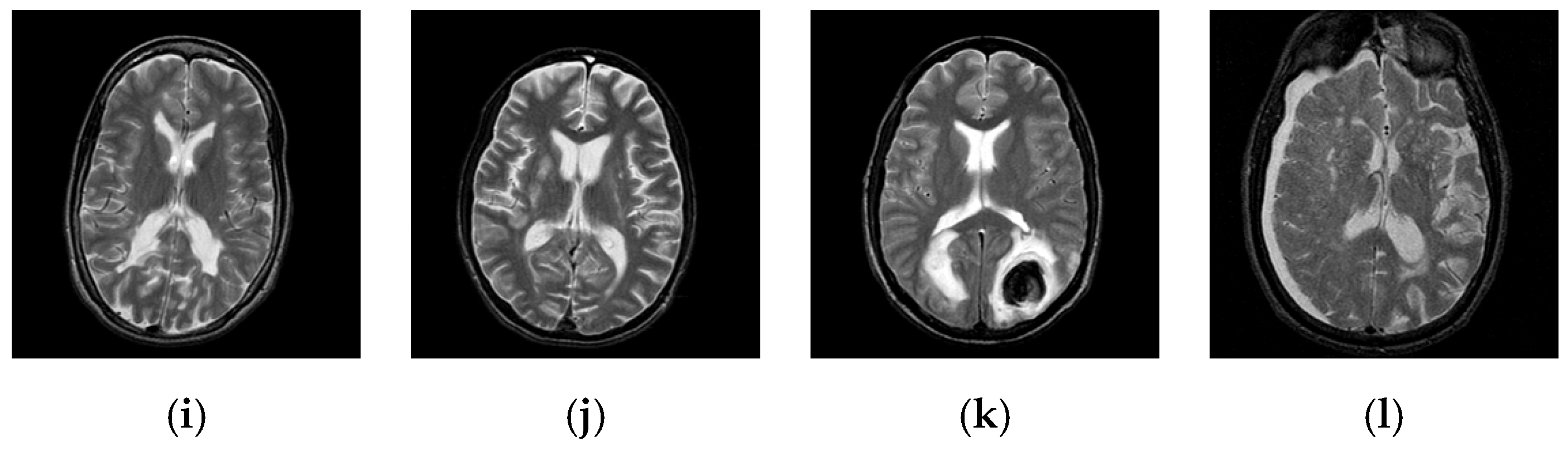
2. Materials
3. Methodology
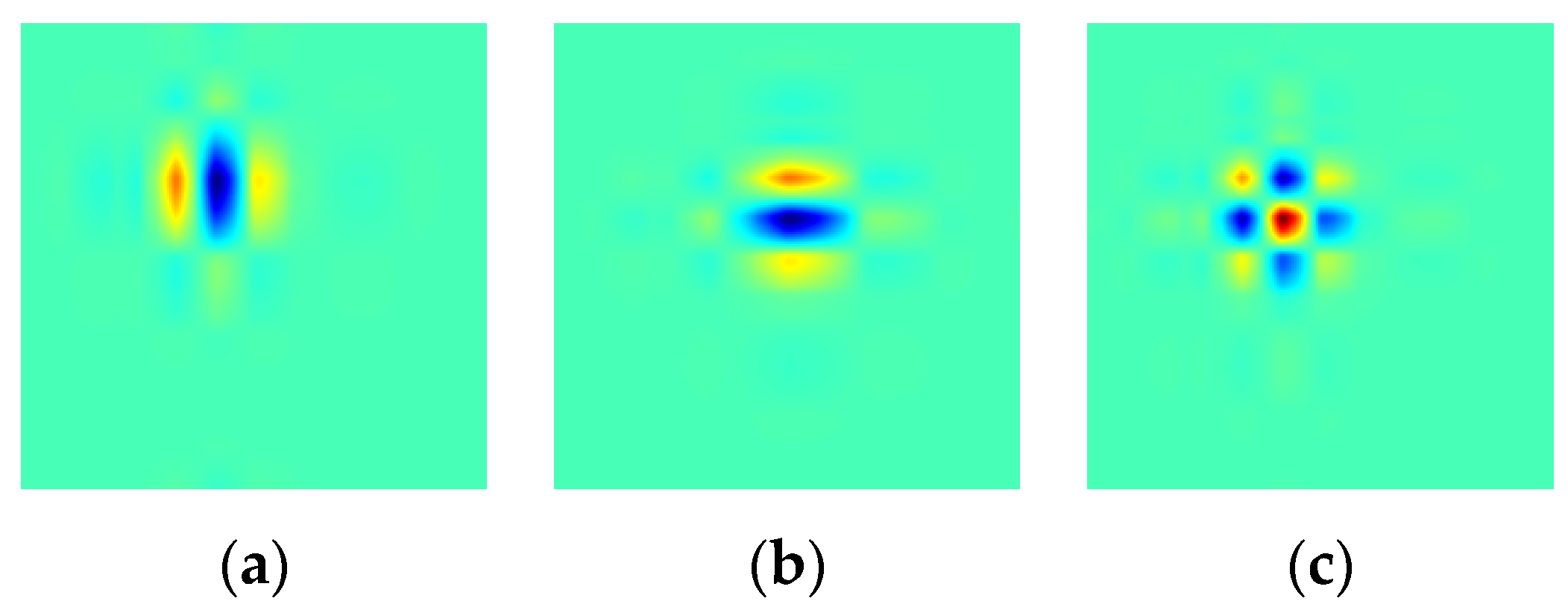
3.1. Discrete Wavelet Transform
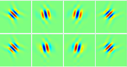
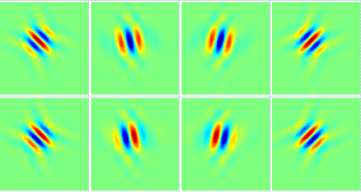
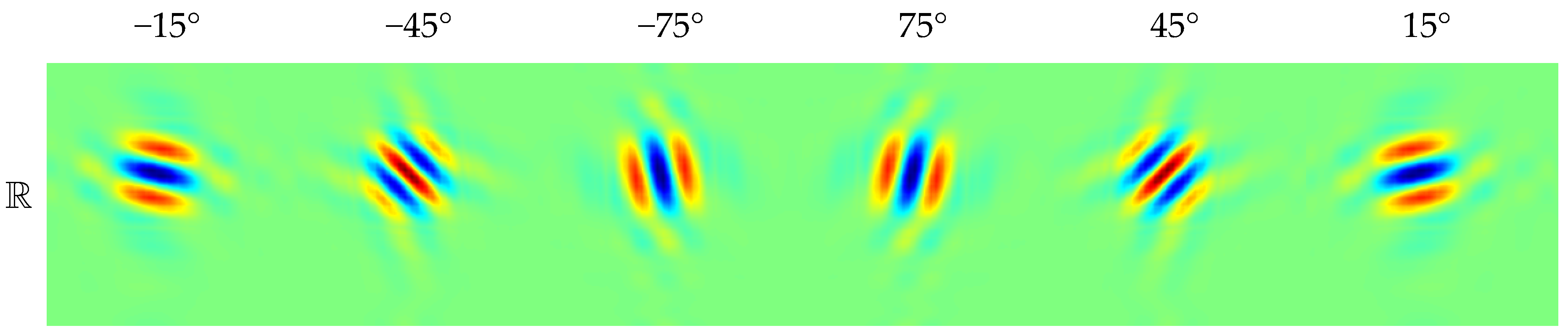
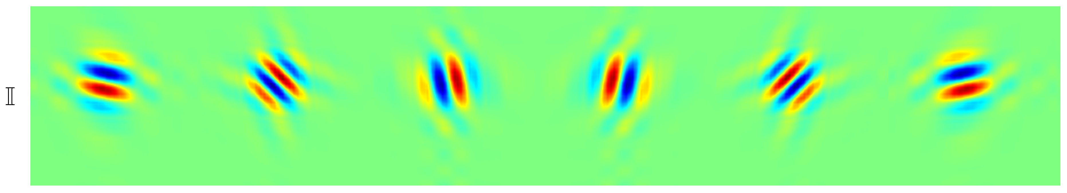
3.2. Dual-Tree Complex Wavelet Transform
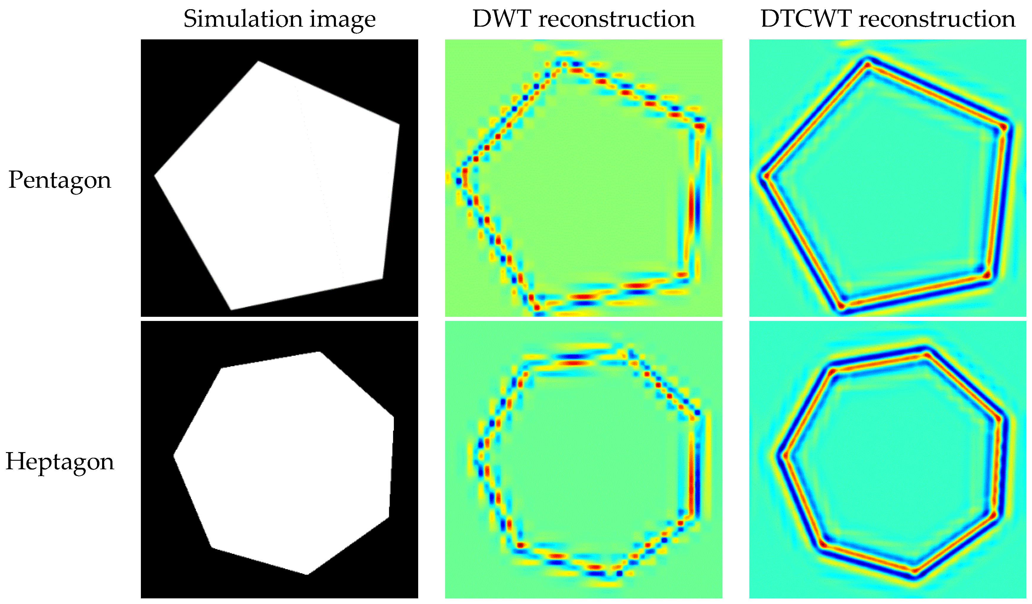
3.3. Comparison between DWT and DTCWT
3.4. Variance and Entropy (VE)
3.5. Generalized Eigenvalue Proximal SVM
3.6. Twin Support Vector Machine
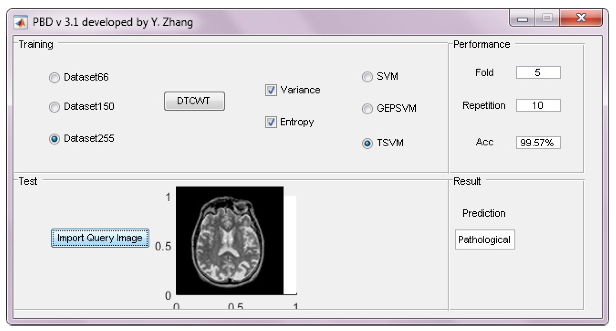
3.7. Pseudocode of the Whole System
4. Experiment Design
4.1. Statistical Setting
4.2. Parameter Estimation for s
4.3. Evaluation
5. Results and Discussions
5.1. Classifier Comparison
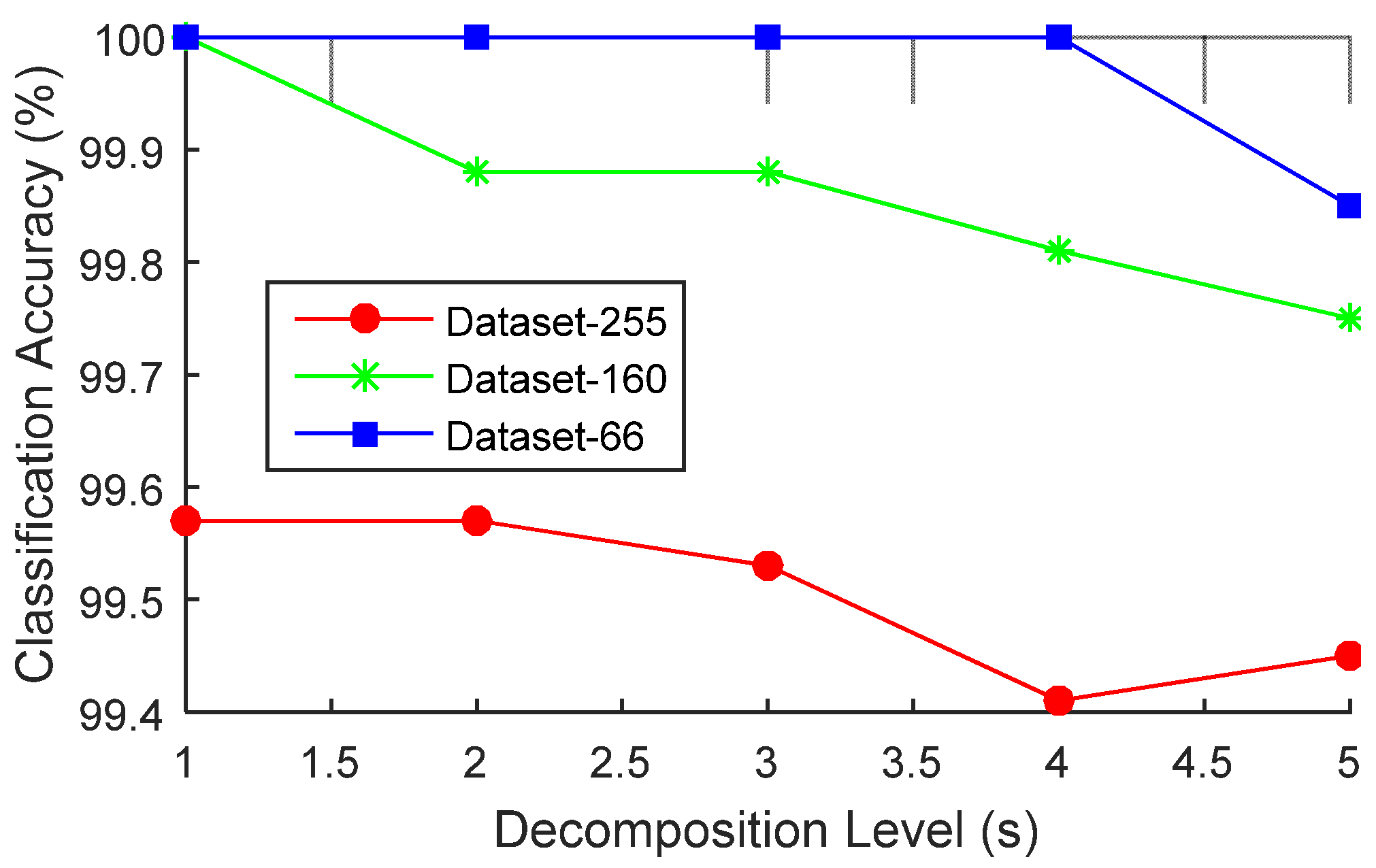
5.2. Optimal Decomposition Level Selection
5.3. Comparison to State-of-the-Art Approaches
5.4. Results of Different Runs
5.5. Computation Time
5.6. Comparison to Human Reported Results
6. Conclusions and Future Research
Acknowledgment
Author Contributions
Conflicts of interest
Abbreviations
| (A)(BP)(F)(PC)NN | (Artificial) (Back-propagation) (Feed-forward) (Pulse-coupled) neural network |
| (B)PSO(-MT) | (Binary) Particle Swarm Optimization (-Mutation and TVAC) |
| (D)(S)W(P)T | (Discrete) (Stationary) wavelet (packet) transform |
| (k)(F)(LS)(GEP)SVM | (kernel) (Fuzzy) (Least-Squares) (Generalized eigenvalue proximal) Support vector machine |
| (W)(P)(T)E | (Wavelet) (Packet) (Tsallis) entropy |
| CAD | Computer-aided diagnosis |
| CS | Cost-sensitivity |
| FRFE | Fractional Fourier entropy |
| HMI | Hu moment invariant |
| KNN | K-nearest neighbors |
| MR(I) | Magnetic resonance (imaging) |
| PCA | Principal Component Analysis |
| RBF | Radial Basis Function |
| TVAC | Time-varying Acceleration Coefficients |
| WTT | Welch’s t-test |
References
- Thorsen, F.; Fite, B.; Mahakian, L.M.; Seo, J.W.; Qin, S.P.; Harrison, V.; Johnson, S.; Ingham, E.; Caskey, C.; Sundstrom, T.; et al. Multimodal imaging enables early detection and characterization of changes in tumor permeability of brain metastases. J. Controll. Release 2013, 172, 812–822. [Google Scholar] [CrossRef] [PubMed]
- Gorji, H.T.; Haddadnia, J. A novel method for early diagnosis of Alzheimer's disease based on pseudo Zernike moment from structural MRI. Neuroscience 2015, 305, 361–371. [Google Scholar] [CrossRef] [PubMed]
- Goh, S.; Dong, Z.; Zhang, Y.; DiMauro, S.; Peterson, B.S. Mitochondrial dysfunction as a neurobiological subtype of autism spectrum disorder: Evidence from brain imaging. JAMA Psychiatry 2014, 71, 665–671. [Google Scholar] [CrossRef] [PubMed]
- El-Dahshan, E.S.A.; Hosny, T.; Salem, A.B.M. Hybrid intelligent techniques for MRI brain images classification. Digit. Signal Process. 2010, 20, 433–441. [Google Scholar] [CrossRef]
- Patnaik, L.M.; Chaplot, S.; Jagannathan, N.R. Classification of magnetic resonance brain images using wavelets as input to support vector machine and neural network. Biomed. Signal Process. Control 2006, 1, 86–92. [Google Scholar]
- Dong, Z.; Wu, L.; Wang, S.; Zhang, Y. A hybrid method for MRI brain image classification. Expert Syst. Appl. 2011, 38, 10049–10053. [Google Scholar]
- Wu, L. An MR brain images classifier via principal component analysis and kernel support vector machine. Prog. Electromagn. Res. 2012, 130, 369–388. [Google Scholar]
- Das, S.; Chowdhury, M.; Kundu, M.K. Brain MR image classification using multiscale geometric analysis of Ripplet. Progress Electromagn. Res.-Pier 2013, 137, 1–17. [Google Scholar] [CrossRef]
- El-Dahshan, E.S.A.; Mohsen, H.M.; Revett, K.; Salem, A.B.M. Computer-Aided diagnosis of human brain tumor through MRI: A survey and a new algorithm. Expert Syst. Appl. 2014, 41, 5526–5545. [Google Scholar] [CrossRef]
- Dong, Z.; Ji, G.; Yang, J. Preclinical diagnosis of magnetic resonance (MR) brain images via discrete wavelet packet transform with Tsallis entropy and generalized eigenvalue proximal support vector machine (GEPSVM). Entropy 2015, 17, 1795–1813. [Google Scholar]
- Wang, S.; Dong, Z.; Du, S.; Ji, G.; Yan, J.; Yang, J.; Wang, Q.; Feng, C.; Phillips, P. Feed-Forward neural network optimized by hybridization of PSO and ABC for abnormal brain detection. Int. J. Imaging Syst. Technol. 2015, 25, 153–164. [Google Scholar] [CrossRef]
- Nazir, M.; Wahid, F.; Khan, S.A. A simple and intelligent approach for brain MRI classification. J. Intell. Fuzzy Syst. 2015, 28, 1127–1135. [Google Scholar]
- Sun, P.; Wang, S.; Phillips, P.; Zhang, Y. Pathological brain detection based on wavelet entropy and Hu moment invariants. Bio-Med. Mater. Eng. 2015, 26, 1283–1290. [Google Scholar]
- Mount, N.J.; Abrahart, R.J.; Dawson, C.W.; Ab Ghani, N. The need for operational reasoning in data-driven rating curve prediction of suspended sediment. Hydrol. Process. 2012, 26, 3982–4000. [Google Scholar] [CrossRef]
- Abrahart, R.J.; Dawson, C.W.; See, L.M.; Mount, N.J.; Shamseldin, A.Y. Discussion of “Evapotranspiration modelling using support vector machines”. Hydrol. Sci. J.-J. Sci. Hydrol. 2010, 55, 1442–1450. [Google Scholar] [CrossRef]
- Si, Y.; Zhang, Z.S.; Cheng, W.; Yuan, F.C. State detection of explosive welding structure by dual-tree complex wavelet transform based permutation entropy. Steel Compos. Struct. 2015, 19, 569–583. [Google Scholar] [CrossRef]
- Hamidi, H.; Amirani, M.C.; Arashloo, S.R. Local selected features of dual-tree complex wavelet transform for single sample face recognition. IET Image Process. 2015, 9, 716–723. [Google Scholar] [CrossRef]
- Murugesan, S.; Tay, D.B.H.; Cooke, I.; Faou, P. Application of dual tree complex wavelet transform in tandem mass spectrometry. Comput. Biol. Med. 2015, 63, 36–41. [Google Scholar] [CrossRef] [PubMed]
- Smaldino, P.E. Measures of individual uncertainty for ecological models: Variance and entropy. Ecol. Model. 2013, 254, 50–53. [Google Scholar] [CrossRef]
- Yang, G.; Zhang, Y.; Yang, J.; Ji, G.; Dong, Z.; Wang, S.; Feng, C.; Wang, Q. Automated classification of brain images using wavelet-energy and biogeography-based optimization. Multimed. Tools Appl. 2015, 1–17. [Google Scholar] [CrossRef]
- Guang-Shuai, Z.; Qiong, W.; Chunmei, F.; Elizabeth, L.; Genlin, J.; Shuihua, W.; Yudong, Z.; Jie, Y. Automated Classification of Brain MR Images using Wavelet-Energy and Support Vector Machines. In Proceedings of the 2015 International Conference on Mechatronics, Electronic, Industrial and Control Engineering, Shenyang, China, 24–26 April 2015; Liu, C., Chang, G., Luo, Z., Eds.; Atlantis Press: Shenyang, China, 2015; pp. 683–686. [Google Scholar]
- Carrasco, M.; Lopez, J.; Maldonado, S. A second-order cone programming formulation for nonparallel hyperplane support vector machine. Expert Syst. Appl. 2016, 54, 95–104. [Google Scholar] [CrossRef]
- Wei, Y.C.; Watada, J.; Pedrycz, W. Design of a qualitative classification model through fuzzy support vector machine with type-2 fuzzy expected regression classifier preset. IEEJ Trans. Electr. Electron. Eng. 2016, 11, 348–356. [Google Scholar] [CrossRef]
- Wu, L.; Zhang, Y. Classification of fruits using computer vision and a multiclass support vector machine. Sensors 2012, 12, 12489–12505. [Google Scholar]
- Johnson, K.A.; Becker, J.A. The Whole Brain Atlas. Available online: http://www.med.harvard.edu/AANLIB/home.html (accessed on 1 March 2016).
- Silver, D.; Huang, A.; Maddison, C.J.; Guez, A.; Sifre, L.; van den Driessche, G.; Schrittwieser, J.; Antonoglou, I.; Panneershelvam, V.; Lanctot, M.; et al. Mastering the game of Go with deep neural networks and tree search. Nature 2016, 529, 484–489. [Google Scholar] [CrossRef] [PubMed]
- Ng, E.Y.K.; Borovetz, H.S.; Soudah, E.; Sun, Z.H. Numerical Methods and Applications in Biomechanical Modeling. Comput. Math. Methods Med. 2013, 2013, 727830:1–727830:2. [Google Scholar] [CrossRef] [PubMed]
- Zhang, Y.; Peng, B.; Liang, Y.-X.; Yang, J.; So, K.; Yuan, T.-F. Image processing methods to elucidate spatial characteristics of retinal microglia after optic nerve transection. Sci. Rep. 2016, 6, 21816. [Google Scholar] [CrossRef] [PubMed] [Green Version]
- Shin, D.K.; Moon, Y.S. Super-Resolution image reconstruction using wavelet based patch and discrete wavelet transform. J. Signal. Process. Syst. Signal Image Video Technol. 2015, 81, 71–81. [Google Scholar] [CrossRef]
- Yu, D.; Shui, H.; Gen, L.; Zheng, C. Exponential wavelet iterative shrinkage thresholding algorithm with random shift for compressed sensing magnetic resonance imaging. IEEJ Trans. Electr. Electron. Eng. 2015, 10, 116–117. [Google Scholar]
- Beura, S.; Majhi, B.; Dash, R. Mammogram classification using two dimensional discrete wavelet transform and gray-level co-occurrence matrix for detection of breast cancer. Neurocomputing 2015, 154, 1–14. [Google Scholar] [CrossRef]
- Ayatollahi, F.; Raie, A.A.; Hajati, F. Expression-Invariant face recognition using depth and intensity dual-tree complex wavelet transform features. J. Electron. Imaging 2015, 24, 13. [Google Scholar] [CrossRef]
- Hill, P.R.; Anantrasirichai, N.; Achim, A.; Al-Mualla, M.E.; Bull, D.R. Undecimated Dual-Tree Complex Wavelet Transforms. Signal Process-Image Commun. 2015, 35, 61–70. [Google Scholar] [CrossRef]
- Kadiri, M.; Djebbouri, M.; Carré, P. Magnitude-Phase of the dual-tree quaternionic wavelet transform for multispectral satellite image denoising. EURASIP J. Image Video Process. 2014, 2014, 1–16. [Google Scholar] [CrossRef]
- Singh, H.; Kaur, L.; Singh, K. Fractional M-band dual tree complex wavelet transform for digital watermarking. Sadhana-Acad. Proc. Eng. Sci. 2014, 39, 345–361. [Google Scholar] [CrossRef]
- Celik, T.; Tjahjadi, T. Multiscale texture classification using dual-tree complex wavelet transform. Pattern Recognit. Lett. 2009, 30, 331–339. [Google Scholar] [CrossRef]
- Zhang, Y.; Wang, S.; Dong, Z.; Phillips, P.; Ji, G.; Yang, J. Pathological brain detection in magnetic resonance imaging scanning by wavelet entropy and hybridization of biogeography-based optimization and particle swarm optimization. Progress Electromagn. Res. 2015, 152, 41–58. [Google Scholar] [CrossRef]
- Mangasarian, O.L.; Wild, E.W. Multisurface proximal support vector machine classification via generalized eigenvalues. IEEE Trans. Pattern Anal. Mach. Intell. 2006, 28, 69–74. [Google Scholar] [CrossRef] [PubMed]
- Khemchandani, R.; Karpatne, A.; Chandra, S. Generalized eigenvalue proximal support vector regressor. Expert Syst. Appl. 2011, 38, 13136–13142. [Google Scholar] [CrossRef]
- Shao, Y.H.; Deng, N.Y.; Chen, W.J.; Wang, Z. Improved Generalized Eigenvalue Proximal Support Vector Machine. IEEE Signal Process. Lett. 2013, 20, 213–216. [Google Scholar] [CrossRef]
- Jayadeva; Khemchandani, R.; Chandra, S. Twin support vector machines for pattern classification. IEEE Trans. Pattern Anal. Mach. Intell. 2007, 29, 905–910. [Google Scholar] [CrossRef] [PubMed]
- Nasiri, J.A.; Charkari, N.M.; Mozafari, K. Energy-Based model of least squares twin Support Vector Machines for human action recognition. Signal Process. 2014, 104, 248–257. [Google Scholar] [CrossRef]
- Xu, Z.J.; Qi, Z.Q.; Zhang, J.Q. Learning with positive and unlabeled examples using biased twin support vector machine. Neural Comput. Appl. 2014, 25, 1303–1311. [Google Scholar] [CrossRef]
- Shao, Y.H.; Chen, W.J.; Zhang, J.J.; Wang, Z.; Deng, N.Y. An efficient weighted Lagrangian twin support vector machine for imbalanced data classification. Pattern Recognit. 2014, 47, 3158–3167. [Google Scholar] [CrossRef]
- Zhang, Y.-D.; Wang, S.-H.; Yang, X.-J.; Dong, Z.-C.; Liu, G.; Phillips, P.; Yuan, T.-F. Pathological brain detection in MRI scanning by wavelet packet Tsallis entropy and fuzzy support vector machine. SpringerPlus 2015, 4, 716. [Google Scholar] [CrossRef] [PubMed]
- Zhang, Y.-D.; Chen, S.; Wang, S.-H.; Yang, J.-F.; Phillips, P. Magnetic resonance brain image classification based on weighted-type fractional Fourier transform and nonparallel support vector machine. Int. J. Imaging Syst. Technol. 2015, 25, 317–327. [Google Scholar] [CrossRef]
- Zhang, Y.; Wang, S. Detection of Alzheimer’s disease by displacement field and machine learning. PeerJ 2015, 3. [Google Scholar] [CrossRef] [PubMed]
- Purushotham, S.; Tripathy, B.K. Evaluation of classifier models using stratified tenfold cross validation techniques. In Global Trends in Information Systems and Software Applications; Krishna, P.V., Babu, M.R., Ariwa, E., Eds.; Springer-Verlag Berlin: Berlin, Germany, 2012; Volume 270, pp. 680–690. [Google Scholar]
- Ng, E.Y.K.; Jamil, M. Parametric sensitivity analysis of radiofrequency ablation with efficient experimental design. Int. J. Thermal Sci. 2014, 80, 41–47. [Google Scholar] [CrossRef]
- Kumar, M.A.; Gopal, M. Least squares twin support vector machines for pattern classification. Expert Syst. Appl. 2009, 36, 7535–7543. [Google Scholar] [CrossRef]
- Zhuang, J.; Widschwendter, M.; Teschendorff, A.E. A comparison of feature selection and classification methods in DNA methylation studies using the Illumina Infinium platform. BMC Bioinform. 2012, 13, 14. [Google Scholar] [CrossRef] [PubMed]
- Shamsinejadbabki, P.; Saraee, M. A new unsupervised feature selection method for text clustering based on genetic algorithms. J. Intell. Inf. Syst. 2012, 38, 669–684. [Google Scholar] [CrossRef]
- Dong, Z.; Liu, A.; Wang, S.; Ji, G.; Zhang, Z.; Yang, J. Magnetic resonance brain image classification via stationary wavelet transform and generalized eigenvalue proximal support vector machine. J. Med. Imaging Health Inform. 2015, 5, 1395–1403. [Google Scholar]
- Yang, X.; Sun, P.; Dong, Z.; Liu, A.; Yuan, T.-F. Pathological Brain Detection by a Novel Image Feature—Fractional Fourier Entropy. Entropy 2015, 17, 7877. [Google Scholar]
- Zhou, X.-X.; Yang, J.-F.; Sheng, H.; Wei, L.; Yan, J.; Sun, P.; Wang, S.-H. Combination of stationary wavelet transform and kernel support vector machines for pathological brain detection. Simulation 2016. [Google Scholar] [CrossRef]
- Sun, N.; Morris, J.G.; Xu, J.; Zhu, X.; Xie, M. iCARE: A framework for big data-based banking customer analytics. IBM J. Res. Dev. 2014, 58, 9. [Google Scholar] [CrossRef]
- Rajeshwari, J.; Karibasappa, K.; Gopalakrishna, M.T. Three phase security system for vehicles using face recognition on distributed systems. In Information Systems Design and Intelligent Applications; Satapathy, S.C., Mandal, J.K., Udgata, S.K., Bhateja, V., Eds.; Springer-Verlag Berlin: Berlin, Germany, 2016; Volume 435, pp. 563–571. [Google Scholar]
- Wang, S.; Yang, M.; Zhang, Y.; Li, J.; Zou, L.; Lu, S.; Liu, B.; Yang, J.; Zhang, Y. Detection of Left-Sided and Right-Sided Hearing Loss via Fractional Fourier Transform. Entropy 2016, 18, 194. [Google Scholar] [CrossRef]
- Shubati, A.; Dawson, C.W.; Dawson, R. Artefact generation in second life with case-based reasoning. Softw. Qual. J. 2011, 19, 431–446. [Google Scholar] [CrossRef]
- Zhang, Y.; Yang, X.; Cattani, C.; Rao, R.; Wang, S.; Phillips, P. Tea Category Identification Using a Novel Fractional Fourier Entropy and Jaya Algorithm. Entropy 2016, 18, 77. [Google Scholar] [CrossRef]
- Ji, L.Z.; Li, P.; Li, K.; Wang, X.P.; Liu, C.C. Analysis of short-term heart rate and diastolic period variability using a refined fuzzy entropy method. Biomed. Eng. Online 2015, 14, 13. [Google Scholar] [CrossRef] [PubMed]
- Li, P.; Liu, C.Y.; Li, K.; Zheng, D.C.; Liu, C.C.; Hou, Y.L. Assessing the complexity of short-term heartbeat interval series by distribution entropy. Med. Biol. Eng. Comput. 2015, 53, 77–87. [Google Scholar] [CrossRef] [PubMed]
- Lau, P.Y.; Park, S. A new framework for managing video-on-demand servers: Quad-Tier hybrid architecture. IEICE Electron. Express 2011, 8, 1399–1405. [Google Scholar] [CrossRef]
- Lau, P.Y.; Park, S.; Lee, J. Cohort-Surrogate-Associate: A server-subscriber load sharing model for video-on-demand services. Malayas. J. Comput. Sci. 2011, 24, 1–16. [Google Scholar]


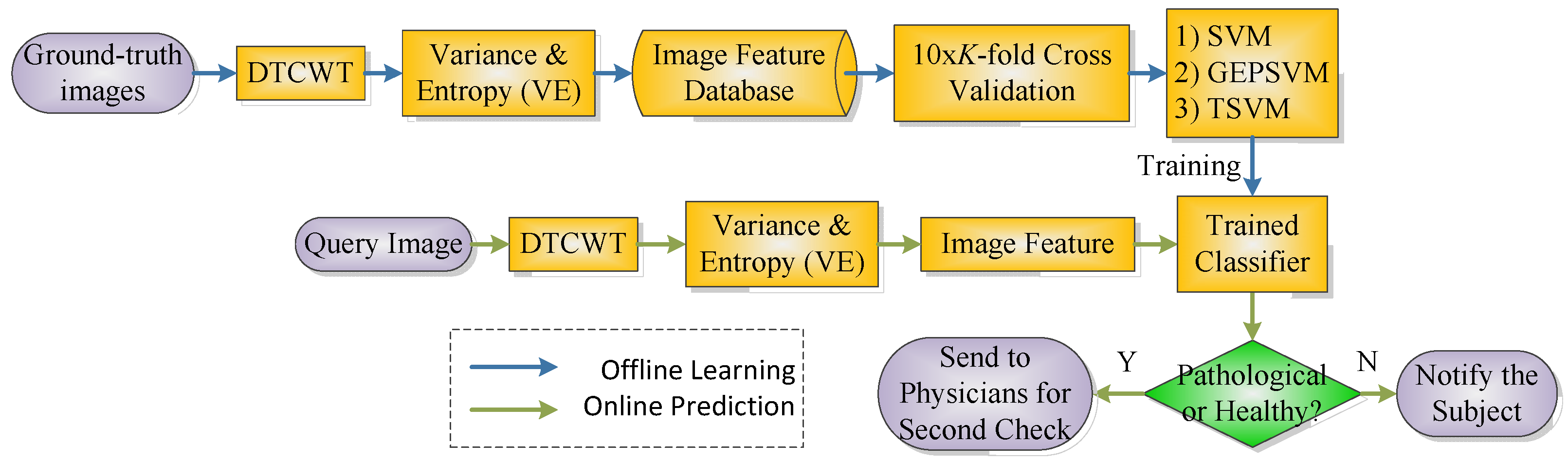
| Phase I: Offline learning | ||
| Step A | Wavelet Analysis | Perform s-level dual-tree complex wavelet transform (DTCWT) on every image in the ground-truth dataset |
| Step B | Feature Extraction | Obtain 12 × s features (6 × s Variances and 6s Entropies, and s represents the decomposition level) from the subbands of DTCWT |
| Step C | Training | Submit the set of features together with the class labels to the classifier, in order to train its weights/biases. |
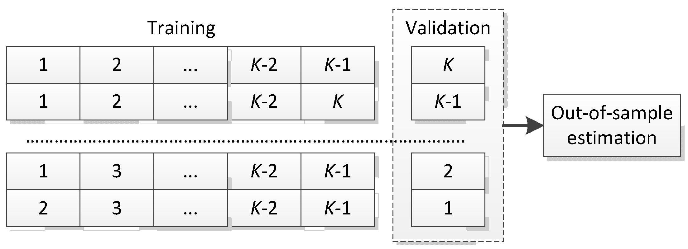
| Step D | Evaluation | Record the classification performance based on a 10 × K - fold stratified cross validation. |
| Phase II: Online prediction | ||
| Step A | Wavelet Analysis | Perform s-level DTCWT on the real query image (independent from training images) |
| Step B | Feature Extraction | Obtain VE feature set |
| Step C | Prediction | Feed the VE feature set into the trained classifier, and obtain the output. |
| Dataset | No. of Fold | Training | Validation | Total | |||
|---|---|---|---|---|---|---|---|
| H | P | H | P | H | P | ||
| Dataset66 | 6 | 15 | 40 | 3 | 8 | 18 | 48 |
| Dataset160 | 5 | 16 | 112 | 4 | 28 | 20 | 140 |
| Dataset255 | 5 | 28 | 176 | 7 | 44 | 35 | 220 |
| Our Methods | Dataset66 | Dataset160 | Dataset255 |
|---|---|---|---|
| DTCWT + VE + SVM | 100.00 | 99.69 | 98.43 |
| DTCWT + VE + GEPSVM | 100.00 | 99.75 | 99.25 |
| DTCWT + VE + TSVM | 100.00 | 100.00 | 99.57 |
| Algorithms | Feature # | Run # | Acc | ||
|---|---|---|---|---|---|
| Dataset66 | Dataset160 | Dataset255 | |||
| DWT + PCA + KNN [4] | 7 | 5 | 98.00 | 97.54 | 96.79 |
| DWT + SVM + RBF [5] | 4761 | 5 | 98.00 | 97.33 | 96.18 |
| DWT + PCA + SCG-FNN [6] | 19 | 5 | 100.00 | 99.27 | 98.82 |
| DWT + PCA + SVM + RBF [7] | 19 | 5 | 100.00 | 99.38 | 98.82 |
| RT + PCA + LS-SVM [8] | 9 | 5 | 100.00 | 100.00 | 99.39 |
| PCNN + DWT + PCA + BPNN [9] | 7 | 10 | 100.00 | 98.88 | 98.24 |
| DWPT + TE + GEPSVM [10] | 16 | 10 | 100.00 | 100.00 | 99.33 |
| SWT + PCA + HPA-FNN [11] | 7 | 10 | 100.00 | 100.00 | 99.45 |
| WE + HMI + GEPSVM [13] | 14 | 10 | 100.00 | 99.56 | 98.63 |
| SWT + PCA + GEPSVM [53] | 7 | 10 | 100.00 | 99.62 | 99.02 |
| FRFE + WTT + SVM [54] | 12 | 10 | 100.00 | 99.69 | 98.98 |
| SWT + PCA + SVM + RBF [55] | 7 | 10 | 100.00 | 99.69 | 99.06 |
| DTCWT + VE + TSVM (Proposed) | 12 | 10 | 100.00 | 100.00 | 99.57 |
| Run | F1 | F2 | F3 | F4 | F5 | Total |
|---|---|---|---|---|---|---|
| 1 | 51(100.00%) | 51(100.00%) | 51(100.00%) | 51(100.00%) | 51(100.00%) | 255(100.00%) |
| 2 | 51(100.00%) | 50(98.04%) | 51(100.00%) | 51(100.00%) | 51(100.00%) | 254(99.61%) |
| 3 | 50(98.04%) | 51(100.00%) | 51(100.00%) | 51(100.00%) | 50(98.04%) | 253(99.22%) |
| 4 | 50(98.04%) | 50(98.04%) | 51(100.00%) | 51(100.00%) | 51(100.00%) | 253(99.22%) |
| 5 | 51(100.00%) | 51(100.00%) | 51(100.00%) | 51(100.00%) | 50(98.04%) | 254(99.61%) |
| 6 | 51(100.00%) | 51(100.00%) | 51(100.00%) | 50(98.04%) | 50(98.04%) | 253(99.22%) |
| 7 | 51(100.00%) | 51(100.00%) | 51(100.00%) | 51(100.00%) | 50(98.04%) | 254(99.61%) |
| 8 | 51(100.00%) | 50(98.04%) | 51(100.00%) | 51(100.00%) | 51(100.00%) | 254(99.61%) |
| 9 | 51(100.00%) | 51(100.00%) | 51(100.00%) | 51(100.00%) | 51(100.00%) | 255(100.00%) |
| 10 | 51(100.00%) | 50(98.04%) | 51(100.00%) | 51(100.00%) | 51(100.00%) | 254(99.61%) |
| Average | 253.9 (99.57%) |
| Process | Time (second) |
|---|---|
| DTCWT | 8.41 |
| VE | 1.81 |
| TSVM Training | 0.29 |
| Process | Time (second) |
|---|---|
| DTCWT | 0.037 |
| VE | 0.009 |
| TSVM Test | 0.003 |
| Neuroradiologist | Accuracy |
|---|---|
| O1 | 74% |
| O2 | 78% |
| O3 | 77% |
| O4 | 79% |
| Our method | 96% |
© 2016 by the authors; licensee MDPI, Basel, Switzerland. This article is an open access article distributed under the terms and conditions of the Creative Commons Attribution (CC-BY) license (http://creativecommons.org/licenses/by/4.0/).
Share and Cite
Wang, S.; Lu, S.; Dong, Z.; Yang, J.; Yang, M.; Zhang, Y. Dual-Tree Complex Wavelet Transform and Twin Support Vector Machine for Pathological Brain Detection. Appl. Sci. 2016, 6, 169. https://doi.org/10.3390/app6060169
Wang S, Lu S, Dong Z, Yang J, Yang M, Zhang Y. Dual-Tree Complex Wavelet Transform and Twin Support Vector Machine for Pathological Brain Detection. Applied Sciences. 2016; 6(6):169. https://doi.org/10.3390/app6060169
Chicago/Turabian StyleWang, Shuihua, Siyuan Lu, Zhengchao Dong, Jiquan Yang, Ming Yang, and Yudong Zhang. 2016. "Dual-Tree Complex Wavelet Transform and Twin Support Vector Machine for Pathological Brain Detection" Applied Sciences 6, no. 6: 169. https://doi.org/10.3390/app6060169