Simulation of Reservoir Sediment Flushing of the Three Gorges Reservoir Using an Artificial Neural Network

Abstract

Reservoir sedimentation and its effect on the environment are the most serious world-wide problems in water resources development and utilization today. As one of the largest water conservancy projects, the Three Gorges Reservoir (TGR) has been controversial since its demonstration period, and sedimentation is the major concern. Due to the complex physical mechanisms of water and sediment transport, this study adopts the Error Back Propagation Training Artificial Neural Network (BP-ANN) to analyze the relationship between the sediment flushing efficiency of the TGR and its influencing factors. The factors are determined by the analysis on 1D unsteady flow and sediment mathematical model, mainly including reservoir inflow, incoming sediment concentration, reservoir water level, and reservoir release. Considering the distinguishing features of reservoir sediment delivery in different seasons, the monthly average data from 2003, when the TGR was put into operation, to 2011 are used to train, validate, and test the BP-ANN model. The results indicate that, although the sample space is quite limited, the whole sediment delivery process can be schematized by the established BP-ANN model, which can be used to help sediment flushing and thus decrease the reservoir sedimentation.

1. Introduction

Building reservoirs on rivers, especially sandy rivers, breaks the natural equilibrium state of flow and sediment conditions, as well as riverbed morphology. The lifting of the water level increases water depth, slows down the current velocity, and thus reduces the sediment carrying capacity of water, leading to a large number of sediment deposits in the reservoir.

The global capacity loss of reservoirs takes up to 0.5%–1% of the total reservoir storage every year, approximately 45 km³ [1]. In addition to capacity loss, which disables the design function of reservoirs such as flood control, power generation, irrigation, and water supply, reservoir sedimentation also shortens the serve life of the reservoir, enlarges the flooded and submerged area upstream, threatens the safety upstream, and impacts navigation. The reduction of outflow sediment also results in erosion of riverbeds downstream, and brings about a series of new problems.

There are plenty of sandy rivers in China. According to incomplete statistics, the annual sediment runoff of 11 main rivers in China is about 16.9 × 10⁸ t [2]. The annual sediment runoff at the Cuntan hydrometric station of the Yangtze River is up to 2.10 × 10⁸ t in the year 2012 [3]. With the construction of more and more large-scale reservoirs, the sedimentation problem has become prominent. The world-renowned Three Gorges Reservoir (TGR) is large multi-objective comprehensive water control project with functions of flood control, power generation, navigation, water supply, and so on. Ever since its design and demonstration phase, the sedimentation problem has been one of the principal concerns. Particle size of both the inflow and outflow sediment of the TGR presents a decreasing tendency, especially after the construction of TGR as well as other large-scale reservoirs upstream. The median particle diameter of the inflow sediment into the TGR is around 0.01–0.011 mm, while that of the outflow sediment is about 0.007–0.009 mm [3]. More than 85% of the inflow sediment particles are within 0.062 mm, and only 3%–7% are larger than 0.125mm. Thus, flushing is believed to be an effective way to transport sediment.

In order to make better use of reservoir release to flush sediment, the relationship between the amount of flushed sediment and its influence factors needs to be studied. However, sedimentation affected by geographical location, topography, geology, climate, and other natural factors, as well as human activities, is a very complex and cross-disciplinary subject. It involves river dynamics, geology, geography and other subjects with immature development. Both the complexity and the immaturity lead to the difficulties of solving the reservoir sedimentation problem. Calculation of sediment erosion and deposition can adopt the mathematical model of flow and sediment. There have been a range of mathematical models presented in previous publications [4,5,6,7,8,9], the theoretical foundation of which are mainly composed of: flow continuity equation, flow motion equation, sediment continuity equation, riverbed deformation equation, and sediment-carrying capacity equation. Establishing and solving a comprehensive set of equations for flow and sediment mathematical models is a complex task with requirements of extensive data to get closed conditions. Currently, many important aspects of the sediment transportation rely on experience and subjective judgment, which is not conducive to close the mathematical model. Furthermore, reservoir sedimentation cannot be generalized with a simple 1D mathematical model, while the 2D and 3D models for sediment transport are only available for short river reach or partial fluvial process issues due to their complex structure, the large number of nodes, and time-consuming computation [10,11,12].

The artificial neural network (ANN) model has the characteristics of parallelism, robustness, and nonlinear mapping. In recent years, ANN has been applied and developed to a certain extent in the simulation of river flow and the calculation of 2D plane flow fields. Dibike et al. [13] combined the ANN theory and the hydrodynamic model; the hydrodynamic model is used to provide learning samples for the ANN model, and the trained ANN is then adopted to predict the navigation depth, and flow motion in some important areas of the 2D flow field, such as water level, flow velocity, flow direction and flow rate. Yang et al. [14] generalized the whole basin into several reservoirs and used the reservoir water balance principle and ANN to simulate the runoff of the Irwell River. The model shows a preferable simulation effect for the daily and monthly runoff time series. The ANN is also adopted to derive operating policies of a reservoir, such as [15,16,17,18]. Neelakantan and Pundarikanthan [19] presented a planning model for reservoir operation using a combined backpropagation neural network simulation–optimization (Hooke and Jeeves nonlinear optimization method) process. The combined approach was used for screening the operation policies. Chandramouli and Deka [20] developed a decision support model (DSM) combining a rule based expert system and ANN models to derive operating policies of a reservoir in southern India, and the authors concluded that DSM based on ANN outperforms regression based approaches.

Although some studies of ANN have been published in both hydrodynamics and reservoir operations, respectively, its research and application on reservoir sediment erosion and deposition is still deficient.

In this study, the BP-ANN model is used to determine the complex non-linear relationship between reservoir sediment flushing efficiency and its influencing factors. On the basis of analysis of 1D unsteady flow and sediment mathematical models, four factors composed of reservoir inflow, incoming sediment concentration, reservoir water level, and reservoir release were selected as the input of the model. As the output of the model, sediment flushing efficiency is used to estimate the simulative and predicting accuracy of the model, which should be as close to the desired values as possible. The historical data of the TGR from 2003 to 2010 are used to train the network, and the data in the year of 2011 is adopted for testing. The results indicate that the established model is able to capture the main feature of the reservoir sediment flushing, especially in the flood season, when the majority of the annual sediment is produced. Although the model can be improved with a larger number of samples, the method is proven to be valid and effective.

2. Methodology

The nonlinear mapping of ANN is able to reflect the complex relationship between multiple independent and dependent variables in reservoir sediment flushing with high simulative accuracy and great feasibility. Considering the computational efficiency and practicality, this study adopts ANN to simulate reservoir sedimentation and predict the amount of flushing sediment with different reservoir operational schedules.

2.1. Influence Factors of the Sediment Flushing

Sediment flushing efficiency of reservoir $\mathsf{\lambda }$ shown in Equation (1) is chosen as the indicator of the flushed sediment:

$$\mathsf{\lambda }=\frac{S_{out}}{S_{in}},$$

(1)

where $\mathsf{\lambda }$ is the reservoir sediment flushing efficiency; $S_{out}$ is the flushed sediment amount out of the reservoir; and $S_{in}$ is the sediment inflow into the reservoir.

Referring to the 1D unsteady flow and sediment mathematical model, the major factors affecting sediment flushing efficiency are selected. The model includes: flow continuity equation as shown in Equation (2), flow motion equation as shown in Equation (3), sediment continuity equation as shown in Equation (4), and the riverbed deformation equation as shown in Equation (5):

$$\frac{\partial Q}{\partial x}+\frac{\partial A}{\partial t}=0,$$

(2)

$$\frac{\partial Q}{\partial t}+\frac{\partial }{\partial t}\left(\frac{Q^2}{A}\right)+gA\frac{\partial H}{\partial x}+g\frac{n^{2}Q\left|Q\right|}{A{R}^{\frac{4}{3}}}=0,$$

(3)

$$\frac{\partial AS}{\partial t}+\frac{\partial QS}{\partial x}=-\mathsf{\alpha }B\mathsf{\omega }\left(S-S_{*}\right),$$

(4)

$${\mathsf{\gamma }}_s\frac{\partial A_s}{\partial t}=\mathsf{\alpha }\mathsf{\omega }B\left(S-S_{*}\right),$$

(5)

where

$$H=L-T,$$

(6)

$$\mathsf{\omega }=\sqrt{{\left(13.95-\frac{\nu }{d}\right)}^2+1.09\frac{{\mathsf{\gamma }}_s}{\gamma }gd}-1.95\frac{\mathsf{\nu }}{d},$$

(7)

$$S_{*}=\mathsf{\kappa }{\left(\frac{U^3}{gR\mathsf{\omega }}\right)}^l,$$

(8)

$\text{and }\mathsf{\gamma }$, ${\mathsf{\gamma }}_s$ are the volume-weight of water and sediment, respectively; d is the sediment grain size; A is the cross-sectional area; R is the hydraulic radius; Q is the flow; B is the cross-sectional width; H is the water head between upstream and downstream; L is the reservoir water level; T is the tailwater elevation; $\mathsf{\alpha }$ is the coefficient of saturation recovery; $\mathsf{\omega }$ is the sediment settling velocity; S is the sediment concentration; $S_{*}$ is the sediment-carrying capacity of flow; $\mathsf{\kappa }$, $l$ are coefficient and exponent; and $\mathsf{\nu }$ is the kinematic coefficient of viscosity.

The sediment inflow into a reservoir differs from month to month. A majority of the sediment comes in flood season with flood, and, in non-flood season, the incoming sediment is far less. To improve the simulative accuracy, the sediment delivery characteristics are studied separately for different time periods in a year. Thus, the parameters regarding the water and sediment properties, such as volume-weight, sediment grain size, and kinematic coefficient of viscosity, are considered to be changeless. For each period, the reservoir operation water level is relatively fixed by the operation rules. Thus, the geometric parameters in Equations (2)–(7), including cross-sectional area, width, and hydraulic radius can also be regarded as constants.

On the basis of the analysis above, it can be seen that the major factors that impact the sediment flushing efficiency of reservoirs include: inflow, sediment inflow, release, and water head.

2.2. Artificial Neural Network (ANN)

2.2.1. Outline of ANN

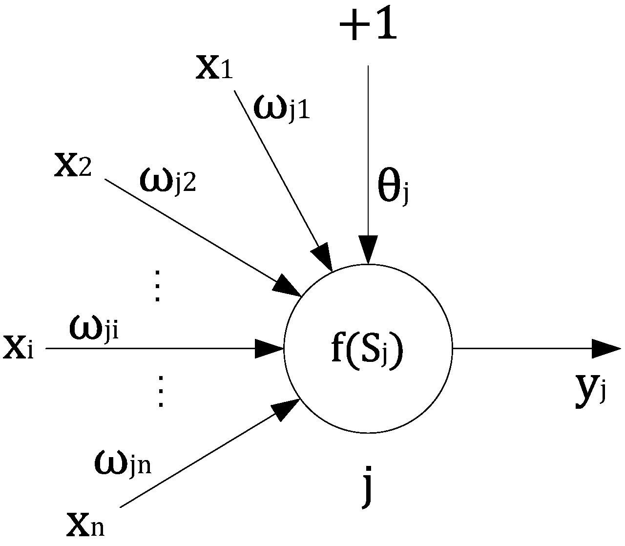
ANN simulates the reaction process of the biological nervous system to information stimulation. To sum up, information processing of neurons consist of two phases: in phase one, the neurons receive information and weight them, known as the integration process; in phase two, the neurons process the integrated information by linear or nonlinear functions, called the activation process. The whole process of inputting information and outputting response can be represented by an activation transfer equation, as shown in Equation (9):

$$Y=F\left({\displaystyle \sum }_{i=1}^n{X}_i{W}_i\right),$$

(9)

where Y is the output of neuron; F is the response characteristic of the neuron to input information; $X_i$ is the input information corresponding to the i-th node; and $W_i$ is the weight of the i-th node.

A neuron is the basic processing unit in neural networks, which is generally a non-linear element with multiple inputs and a single output. Besides being affected by external input signals, the output of a neuron is also influenced by other factors inside the neuron, so an additional input signal $\mathsf{\theta }$ called bias or threshold is often added in the modeling of artificial neurons. Figure 1 describes the information processing of a single neuron mathematically, where j is the index of the neuron.

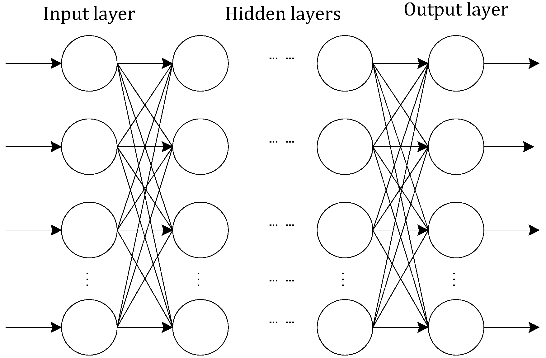
A neural network is composed of an input layer, several hidden layers and an output layer, and there are a certain number of neurons in each layer, which are also called nodes.

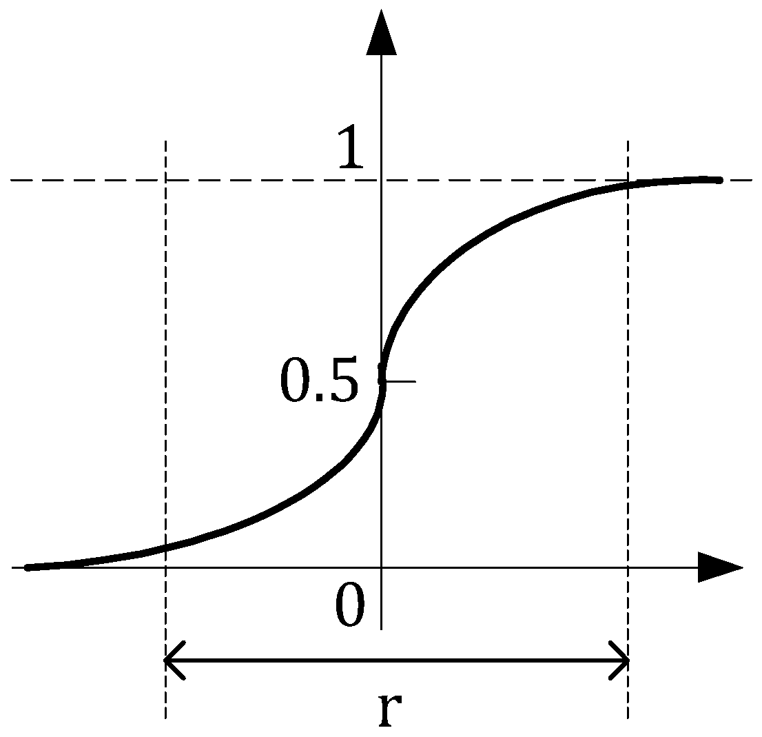
Neuron mapping between different layers is realized by the activation transfer function. The activation transfer function converts the input in an unlimited domain to output within a limited range. A typical activation transfer function includes: threshold function, linear function, S-type function, hyperbolic tangent function, and so on. The domain divided by an S-type activation transfer function is composed of non-linear hyperplanes, which has a soft, smooth, and arbitrary interface. Thus, it is more precise and rational than the linear function with better robustness. Furthermore, since the S-type function is continuously differentiable, it can be strictly calculated by a gradient method. Equation (10) presents the S-type function:

$$f\left(x\right)=\frac{1}{1+e^{-tx}}.$$

(10)

2.2.2. Error Back Propagation Training (BP)-ANN

Neural network algorithms can be classified into the Error Back Propagation Training (BP)-ANN model, the perceptron neural network model, the Radial Basis Function (RBF) neural network model, the Hopfield feedback neural network model, the self-organizing neural network model, and so on. Since it successfully solved the weight adjustment problem of the multilayer feedforward neural network for non-linear continuous functions, the BP-ANN is widely used. Figure 2 shows a mathematical model of the BP-ANN, in which j is the index of the nodes.

BP-ANN is based on gradient search technology with two processes: forward propagation process of information and back propagation process of errors. In forward propagation, the input signal passes through the hidden layers to the output layer. If desired output appears, the learning algorithm ends; otherwise, it turns to back propagation. In back propagation, the error transits through the output layer, and the weights of each layer of neurons are adjusted according to the gradient descent method to reduce the error. Such loop computation continues to make the output of the network approach the expected values as close as possible. Due to its strong nonlinear mapping ability, BP-ANN is used in this study to establish the relationships between the reservoir flushed sediment and its influence factors, the calculation steps of which are illustrated below.

Assuming the input vector is u, the number of neurons in input layer is n, the output vector is y, the number of neurons in the output layer is m, the length of the input/output sample pair is $\overline{L}$, and the steps of the BP-ANN algorithm include:

(1)

Setting the initial weight $\omega \left(0\right)$, which is relatively small random nonzero value;

(2)

Giving the input/output sample pair, and calculating the output of the neural network:

Assuming the input of the p-th sample is $u_p=\left(u_{1p},u_{2p},\dots ,u_{np}\right),$ the output of the p-th sample is $d_p=\left(d_{1p},d_{2p},\dots ,d_{mp}\right),$ p = 1, 2, ..., $\overline{L}$, the output of node i with p-th sample is $y_{ip}$:

$$y_{ip}\left(t\right)=f\left[x_{ip}\left(t\right)\right]=f\left[{\displaystyle \sum }_j{\omega }_{ij}\left(t\right)I_{jp}\right],$$

(11)

where $I_{jp}$is the j-th input of node i when inputting the p-th sample, and f(●) is the activation transfer function as shown in Equation (10);

(3)

Calculating the objective function J of the network:

Assuming $E_p$ is the objective function of the network when inputting the p-th sample, then:

$$E_p=\frac{1}{2}{\displaystyle \sum }_k{\left[d_{kp}-y_{kp}\left(t\right)\right]}^2=\frac{1}{2}{\displaystyle \sum }_k{e}_{kp}^2\left(t\right),$$

(12)

where $y_{kp}$ is the network output after t times of weight adjustment when inputting the p-th sample and k is the index of the node in output layer;

The overall objective function of the network is used to estimate the training level of the network, as shown in Equation (13):

$$J\left(t\right)={\sum }_p{E}_p\left(t\right).$$

(13)

(4)

Discriminating whether the algorithm should stop: if $J\left(t\right)<\mathsf{\epsilon },$ it stops; otherwise, it turns to step (5), where $\mathsf{\epsilon }>0$ is preset;

(5)

Back propagation calculating:

Starting from the output layer, referring to J, do the calculation according to the gradient descent algorithm to adjust the value of weight. Assuming the step length is constant, the (t + 1)-th adjusted weight of the connection from neuron j to neuron i is:

$${\omega }_{ij}\left(t+1\right)={\omega }_{ij}\left(t\right)-\eta \frac{\partial J\left(t\right)}{\partial {\omega }_{ij}\left(t\right)}={\omega }_{ij}\left(t\right)-\eta {\displaystyle \sum }_p\frac{\partial E_p\left(t\right)}{\partial {\omega }_{ij}\left(t\right)}={\omega }_{ij}\left(t\right)+\Delta {\omega }_{ij}\left(t\right),$$

(14)

where $\eta$ is the step length, also called the learning operator,

$$\frac{\partial E_p}{\partial {\omega }_{ij}}=\frac{\partial E_p}{\partial x_{ip}}\cdot \frac{\partial x_{ip}}{\partial {\omega }_{ij}},$$

(15)

$${\delta }_{ip}=\frac{\partial E_p}{\partial x_{ip}},$$

(16)

where ${\mathsf{\delta }}_{ip}$ is the sensitivity of the status of the i-th node $x_{ip}$ to $E_p$ when inputting the p-th sample. Equation (17) can be derived from Equation (15) to Equation (16):

$$\frac{\partial E_p}{\partial {\omega }_{ij}}={\delta }_{ip}{I}_{jp}.$$

(17)

Calculating ${\mathsf{\delta }}_{ip}$ in two different conditions:

①

If i is output node, i.e., i = k, it can be derived from Equations (12) and (16) that

$${\delta }_{ip}={\delta }_{kp}=\frac{\partial E_p}{\partial x_{kp}}=\frac{\partial E_p}{\partial y_{kp}}\cdot \frac{\partial y_{kp}}{\partial x_{kp}}=-e_{kp}{f}^{\prime }\left(x_{kp}\right).$$

(18)

Substitute Equation (18) into Equation (15), then

$$\frac{\partial E_p}{\partial {\omega }_{ij}}=-e_{kp}{f}^{\prime }\left(x_{kp}\right)I_{jp}.$$

(19)

②

If i is not an output node, i.e., i$\ne$k, Equation (16) is:

$${\delta }_{ip}=\frac{\partial E_p}{\partial x_{ip}}=\frac{\partial E_p}{\partial y_{ip}}\cdot \frac{\partial y_{ip}}{\partial x_{ip}}=\frac{\partial E_p}{\partial y_{ip}}\cdot f^{\prime }\left(x_{ip}\right),$$

(20)

in which

$$\frac{\partial E_p}{\partial y_{ip}}={\sum }_{m_1}\frac{\partial E_p}{\partial x_{m_{1}p}}\cdot \frac{\partial x_{m_{1}p}}{\partial y_{ip}}={\sum }_{m_1}\frac{\partial E_p}{\partial x_{m_{1}p}}\cdot \frac{\partial {\sum }_j{\omega }_{m_{1}j}{I}_{jp}}{\partial y_{ip}}={\sum }_{m_1}\frac{\partial E_p}{\partial x_{m_{1}p}}\cdot {\omega }_{m_{1}i}={\sum }_{m_1}{\delta }_{m_{1}p}\cdot {\omega }_{m_{1}i},$$

(21)

where $m_1$ is the $m_1$-th node in the layer after node i; $I_{jp}$ is the j-th input for node i. When i = j, $y_{jp}=I_{jp}$. Substitute Equations (20) and (21) into Equation (15), then

$$\frac{\partial E_p}{\partial {\omega }_{ij}}=f\left(x_{ip}\right)I_{jp}{\displaystyle \sum }_{m_1}\frac{\partial E_p}{\partial x_{m_{1}p}}\cdot {\omega }_{m_{1}i}=f\left(x_{ip}\right)I_{jp}{\displaystyle \sum }_{m_1}{\delta }_{m_{1}p}\cdot {\omega }_{m_{1}i}.$$

(22)

Equations (19) and (22) can be used to adjust the weight in Equation (14).

The expression of BP-ANN mapping is a compound of a simple nonlinear function. Several such compound is able to represent complex functions, and then describe many complex processes in physical phenomena.

2.2.3. BP-ANN Model of Reservoir Sedimentation

When combining reservoir sedimentation calculation and reservoir operation, the computational process and constraints are complex, and the time scale is difficult to match. The nonlinear mapping ability of BP-ANN can reflect such complicated relationships between multiple independent and dependent variables without requirements of time-consuming computations.

The sediment flushing efficiency shown in Equation (1) is selected as the output of the BP-ANN model. Based on the analysis in Section 2.2.1, its main influencing factors in real time include: inflow upstream Q_in, sediment concentration upstream S, release flow downstream Q_out, and reservoir water level L, which are the inputs of the BP-ANN model. Taking the TGR reservoir as an example, a BP-ANN model to simulate and predict the reservoir sediment flushing is established with the observed data from 2003, when the TGP was put into operation, to 2011.

3. Results and Discussion

Hecht-Nielsen [21] proved that for any mapping G from closed unit cube in n-dimensional Euclidean space [0,1]ⁿ to m-dimensional Euclidean space R^m in L₂ (we say a function belongs to L2 if each of its coordinate functions is square-integrable on the unit cube), there exists a three-layer BP neural network, which is capable of approaching G with arbitrary precision. Bourquin et al. [22] believed that the Multiple Layer Perception (MLP) with only one hidden layer is sufficient in theory, and, compared to three layers, ANN with four layers is more likely to fall into local optima and harder to train, both of them are similar in other aspects. Hence, BP-ANN model with three layers is selected in this study.

In the application of ANN, it is difficult but crucial to determine an appropriate number of neurons in hidden layer. If the number is too small, the accuracy of the ANN cannot be guaranteed; while if the number is too large, not only the number of connection weights in the network increases, but also the generalization performance of the network is likely to drop. Hence, in this study, the number of neurons in hidden layer is set to be 10.

Input parameters are firstly normalized to fall into [0,1], as shown in Equation (23):

$$\overline{x_i}=\frac{x_i-x_{min,i}}{x_{max,i}-x_{min,i}}.$$

(23)

To prevent supersaturation of the neurons, only a certain range r of the S-type activation transfer function with larger curvature is used for mapping, as illustrated in Figure 3.

Thus, Equation (23) is converted as:

$$\overline{x_i}=\frac{x_i-x_{min,i}\left(1+d_1\right)}{x_{max,i}\left(1+d_2\right)-x_{min,i}\left(1+d_1\right)}.$$

(24)

After several testing trials of calculation, $d_1=40\%$ and $d_2=20\%$ in this study.

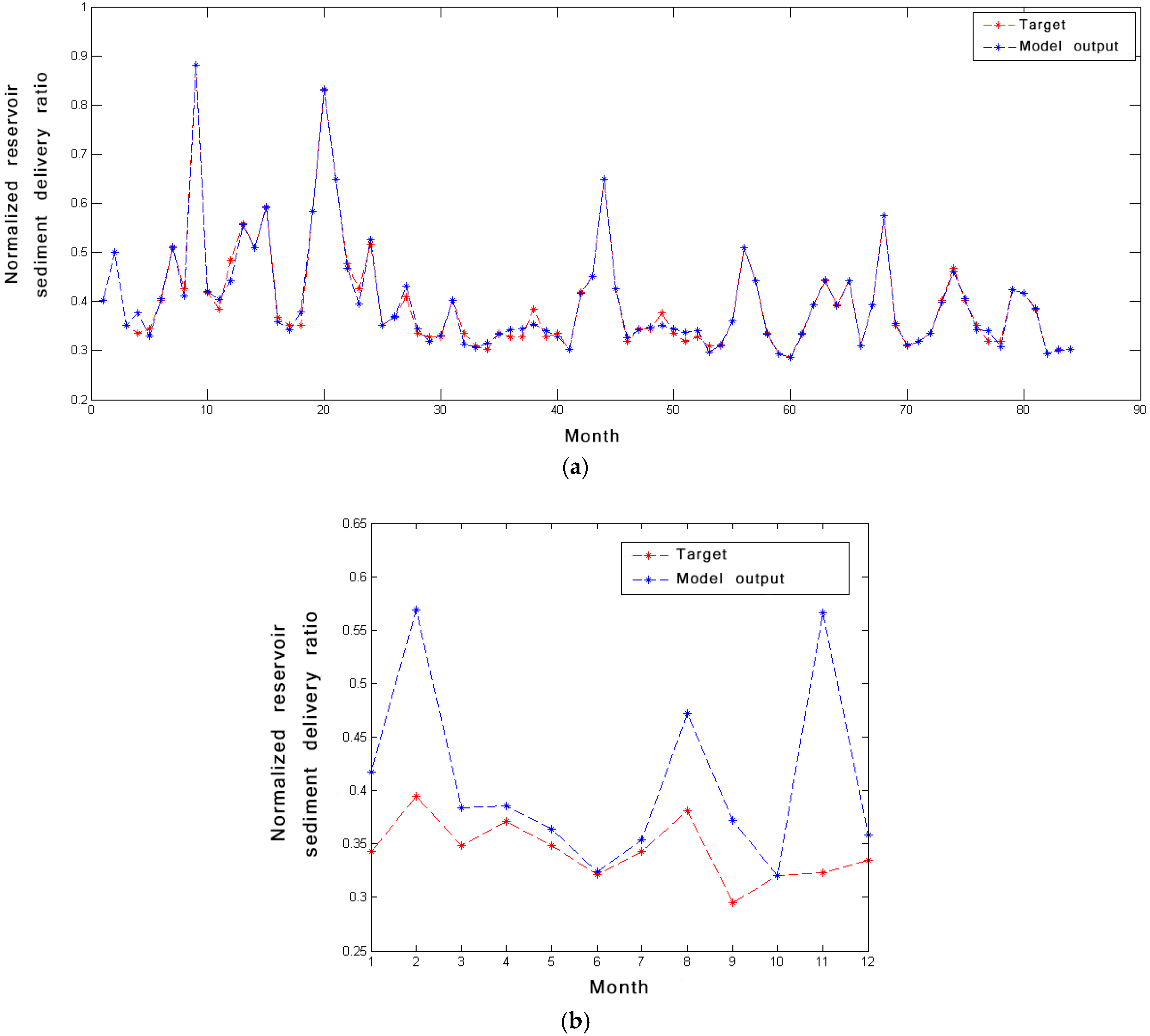
The four types of observed data ($\overrightarrow{Q_{in}},\overrightarrow{Q_{out}},\overrightarrow{L},\overrightarrow{S}$) and the observed sediment flushing efficiency of the TGR from the year 2003 to 2010 are used to train the BP-ANN model, and the data of the year 2011 is used to test it. The simulation and prediction results of the model are shown in Figure 4.

It can be seen from Figure 4 that the trained BP-ANN model can simulate the reservoir sediment flushing process with a high accuracy. When it comes to prediction, the BP-ANN model is able to reflect the relational characteristics of the reservoir sediment flushing. However, since the TGR has only been in operation for about 10 years, and the monthly data is available from 2003 to 2011, the samples used to train the BP-ANN are quite limited, and some deviations still exist. In addition, the sediment delivery from reservoir is an extremely complex process relevant to multiple influencing factors. The reservoir sediment flushing model itself is approximate with many empirical parameters. The four factors selected in this study are necessary and dominated but not sufficient. Last but not least, the majority of the sediment flows into the reservoir in flood season, and very little sediment comes in non-flood season. The difference between the sediment inflow can be several orders of magnitude in different seasons. The observed errors of sediment in the non-flood season itself is not as small as that in flood season. Synthesizing all the reasons above, the BP-ANN model established in this study is believed to be able to characterize the relationship between reservoir flushing sediment and its major influencing factors, especially in flood season, when most of the sediment comes.

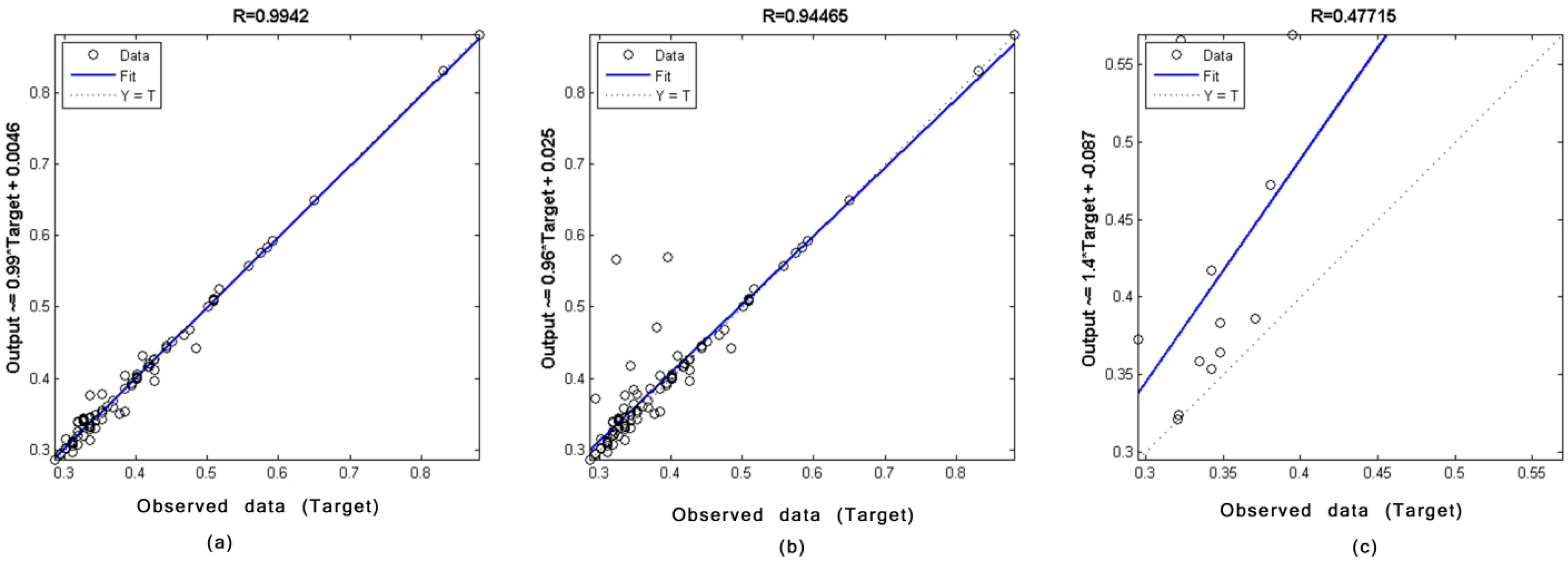
Figure 5 shows the goodness of fit between the model output and the observed data. A satisfying fitting degree can be achieved using only the trained data. For the test, the actual data distributes on both sides of the fit line. Basically, the predicted results from the BP-ANN model is a little larger than the actual data, while the gap is limited.

The statistics of the relative error between the model output and the actual data are shown in Figure 6. There are 96 output variables of the BP-ANN model in the training phase and 12 outputs in testing phase, as the output is monthly sediment flushing efficiency. The blue and green bars in Figure 6 indicate the number of variables with the error falling into a certain range in the training and testing phase, respectively. The red line represents 0 errors occuring. It can be seen that most of the trained outputs stick around the 0 error line. As for the tested outputs, the largest error is about 20%. However, there are only two tested outputs with the error larger than 10%, i.e., over 80% of the predicted sediment flushing efficiency is within 10% difference from the historical data.

As the essential feature can be captured by the BP-ANN model established in this study, it can be inferred that the BP-ANN can be trained with higher prediction accuracy with more samples.

4. Conclusions

Due to the complexity of the reservoir sedimentation process and the immaturity of the sediment research, the calculation of the reservoir sediment erosion and deposition has relied on complicated differential equations with abundant empirical parameters. Since the BP-ANN model has a strong ability to deal with complex non-linear mapping with simpler calculations, it is adopted in order to study the relationships between reservoir flushing sediment and its influencing factors. Four major factors impacting the reservoir sediment flushing efficiency are determined by the analysis on 1D unsteady flow and sediment mathematical model, which are reservoir inflow, water level, outflow, and the inflow sediment concentration. The observed data of the Three Gorges Reservoir from 2003 when it was put into operation to 2010 are used to train the BP-ANN model, and the data of the year 2011 is used for testing. The results show that the established BP-ANN model is able to reflect the essential relationship between the sediment flushing and its influencing factors, especially in flood season, when the majority of the sediment inflows. To improve the accuracy of the model, more observed data is needed in the future.