Simulation Model for Correction and Modeling of Probe Head Errors in Five-Axis Coordinate Systems

Abstract

Simulative methods are nowadays frequently used in metrology for the simulation of measurement uncertainty and the prediction of errors that may occur during measurements. In coordinate metrology, such methods are primarily used with the typical three-axis Coordinate Measuring Machines (CMMs), and lately, also with mobile measuring systems. However, no similar simulative models have been developed for five-axis systems in spite of their growing popularity in recent years. This paper presents the numerical model of probe head errors for probe heads that are used in five-axis coordinate systems. The model is based on measurements of material standards (standard ring) and the use of the Monte Carlo method combined with select interpolation methods. The developed model may be used in conjunction with one of the known models of CMM kinematic errors to form a virtual model of a five-axis coordinate system. In addition, the developed methodology allows for the correction of identified probe head errors, thus improving measurement accuracy. Subsequent verification tests prove the correct functioning of the presented model.

1. Introduction

The development of production engineering and the demand for high quality manufacturing brings about new challenges in the coordinate metrology, which serves as the key tool for quality assurance systems in many branches of industry (automotive, aerospace, machine, etc.) [1,2,3]. With the increase in manufacturing accuracy, the measurements and methods used for assessing measurement uncertainty have to be more precise. The time spent on performing measurements and evaluations also plays a crucial role, as it has a fairly significant impact on the total costs of manufacturing. Therefore, new solutions are being introduced in regards to both the construction of measuring systems, and the methods for the assessment of coordinate measurement accuracy [4,5].

Simulative models constitute one of the newest developments in accuracy estimation. In practice, such models are based on developing virtual models of measuring systems. Their main advantage is the possibility to obtain measurement uncertainty following only a single measurement, whereas the common methods of uncertainty estimation (such as the calibrated workpiece method [6,7], or multiple measurement strategy [8,9]) would require multiple measurements. In some instances, simulative models may also be used for error compensation, and consequently, for improving measurement accuracy.

The virtual Coordinate Measuring Machine (CMM) model was first developed in the 1990s at Physikalisch-Technische Bundesanstalt in Germany [10,11]. The original model was based on the determination of all possible error causes in the entire measuring volume of the CMM, and the evaluation of their impact on measurement results. Thanks to this, the mathematical model of ideal measurement was supplemented by the influence of possible errors that may occur during measurements, and used for performing multiple simulations of the considered measurement. Measurement uncertainty was then determined based on the variability of simulated results and simple statistical operations.

So far, several models have been developed for typical three-axis CMMs. All of those models utilize a similar working principle as the PTB model, and were presented in detail in [12,13,14,15,16,17]. Lately, a virtual model of measurements performed on the Articulated Arm CMM was also developed [18]. Further works focused on the construction of a virtual model for the Laser Tracker system are currently in progress both in Germany and the UK.

In the last years, it has been possible to observe an increase in the popularity of the so-called five-axis coordinate systems. The five-axis system is created by adding two rotations of a probe head to the standard movements of the machine. Thanks to this solution, it is possible to speed up the measuring process, especially for solids of revolution such as rings, cylinders, spheres, etc., without accuracy loss. Workpieces of this type may be measured using mainly movements of the probe head kinematic pairs. Unlike the three-axis CMM, there is no need to move the whole body of the machine during measurements of all points. The reduction in measurement time is clearly visible, and because of that, the number of installations or retrofits for five-axis systems is becoming a fairly common trend in the industry. Nevertheless, hardly any literature can be found on this subject, and few scientists pay sufficient attention to this type of system. For this reason, the authors decided to investigate the field of errors of probe heads used in five-axis systems, and to attempt to develop a model of this type.

The main sources of errors occurring during coordinate measurements performed on a CMM are kinematic system errors and probe head errors [19,20,21,22]. These types of errors are included in all virtual models of CMMs. The models of probe head errors are usually based on error identification with the use of material standards, such as spherical standards and standard rings. Some currently used probe head error simulation models are described below.

A probe head error model utilizing an artificial neural network was developed at the Laboratory of Coordinate Metrology (LCM) of the Cracow University of Technology as part of a Virtual CMM based on assumptions of the matrix method [16]. The model utilizes the Probing Error Function (PEF) described in [13,16]. Probing Error (PE) depends on a number of factors, among them: deformation of the measuring ball during contact, deflection of the stylus under the force of the measurement, probe pretravel, the form error of the measuring ball, non-linearity and differentiation of the transducer characteristics in different directions of deflection, i.e., the directions of probe head movements (u, v, w), reaction to uneven load of the probe head, etc. The PE can be defined as a sum of a number of contributing factors. The value of PE changes significantly for different probing directions, so the PEF may be obtained in relation to the probe deflection angle (α). Values of PEF can be determined through measurements of calibrated material standards with known form deviations. The value of the PE at a certain measured point, measured at a specified angle, may be expressed as a radial error obtained during point measurement [16].

The model is divided into two modules: one responsible for systematic error simulation and the second for random error modeling. The ring gauge of a 25 mm diameter has to be measured 32 times, in 64 evenly distributed points, to gather data for model preparation. It was assumed that the 64 measured points are sufficient to model the probe head functioning for any probing direction. On the basis of obtained results, the mean value of the PEF should be attributed to each measured point. These values are treated as a systematic part of the probing system error. The obtained data is used as a learning data set for the constructed artificial neural network, which links the probe head deflection angle and systematic error. The network consists of three layers, and utilizes back propagation and different activation functions (Figure 1). The module was prepared both for inner dimensions—using the gauge ring as a reference—and outer dimensions. In the case of the latter, the entire procedure should be repeated, except that instead of a ring, the spherical standard of a 25 mm diameter should be measured at the reference sphere equator.

The second module is responsible for a simulation of probe head random errors. The chi-squared test should be used to check the distribution of results obtained during the gauge ring measurement. Tests performed previously indicated that the resulting distributions are mostly similar to a normal distribution. In this case, the random error of the probe head connected with a certain probing direction could be modeled using the standard deviation obtained for the considered point. In order to interpolate the values of standard deviation between measured points, the artificial neural network with identical construction to the one in the previous case was used. Finally, a normal distribution generator based on the Monte Carlo method may be used in order to simulate the random error. More details regarding this model may be found in [16].

Another probe head error model developed at LCM is based on the Monte Carlo method. The main idea of the model is the same as in the previously discussed model, namely to link probe head errors with the probing direction; however, this model was adapted to describe the probe spatial approach to the measured surface. In such a situation at least two angles defining tip deflection should be used to sufficiently describe the probe head behavior. Assuming that deflection can be described similarly to the definition of coordinates in a spherical coordinate system, the final probe head error function (PEF) can be written in the following form in Equation (1) [13]:

PEF = (α, β, PE)

(1)

The standard used during the model preparation stage is the calibration sphere which fulfills the requirements formulated in [13]. The sphere is measured in evenly distributed points on the upper hemisphere of the standard. These points define the nodes of the reference grid of the model, in which probe head errors are determined empirically through measurements. The arrangement of the points can be described using angles (α, β). The sphere is measured at least 10 times, and on the basis of the acquired results the mean value of the PEF at each point is calculated, as well as standard deviation associated with it. Then, a t-distribution described by $\overline{x}$, s, ν parameters is assigned to each grid node, where $\overline{x}$ is the mean value of the distribution, equal to the mean value of the PEF, s is the dispersion equal to the calculated standard deviation, and ν is the number of degrees of freedom equal to the number of measurements minus one. When the direction is different than the one for which errors were determined experimentally, the bilinear interpolation adapted for the spherical system must be used in order to determine the values describing the probability distribution.

The value of the PE for the chosen probing direction is simulated using the Monte Carlo method. Since the PE can be treated as a vector with the same direction as a probing direction, it is possible to calculate its effect on the coordinates of measured points. The probing errors along axes x, y, z of a machine’s datum system (PE_x, PE_y, PE_z) can be expressed as follows:

PE_x = PEF × nx

(2)

PE_y = PEF × ny

(3)

PE_z = PEF × nz

(4)

where:

• nx, ny, nz—approach direction cosines
• PEF—value of probe head error function

The experiment described in [23] was conducted to check the number of points that should be included in the reference grid. As a result, it was found that the model based on 46 points accurately describes the probe errors. More details regarding this model can be found in [13].

The modules presented above served as a starting point for adapting the probe error function to describe the field of errors of the probe heads utilized on five-axis coordinate systems.

2. Developed Simulative Model and Steps to Its Implementation

This section describes the concept of the developed simulative model, and the experiments that were designed and performed in order to implement this model and verify its reliability.

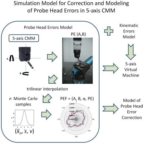
2.1. Description of Simulative Model

The developed simulative model is based on the concept of PEF described in Section 1. In this case, the number of input quantities that has to be specified in order to obtain the probe error (PE) is equal to three. The PEF may be written as presented in Equation (5):

PEF = (A, B, α, PE)

(5)

where:

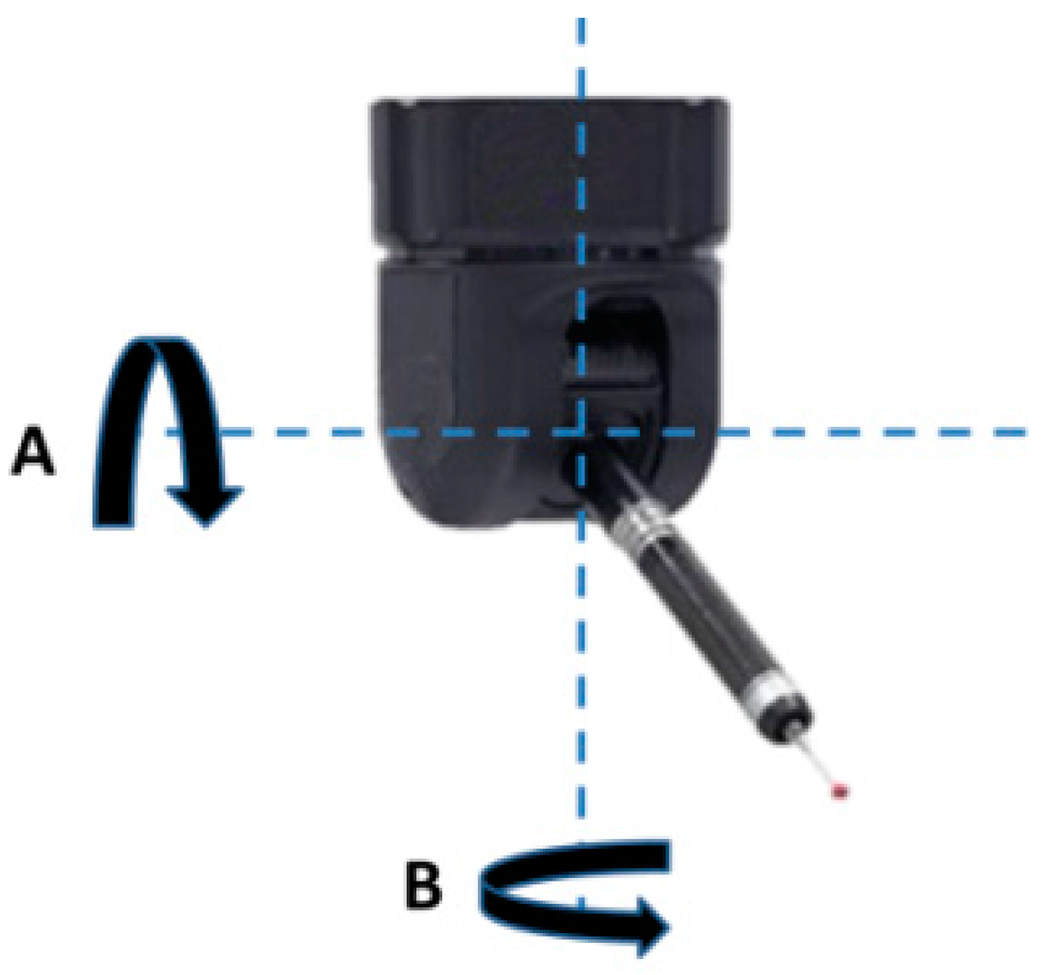
• A—rotation angle along the horizontal axis of the probe head,
• B—rotation angle along the vertical axis of the probe head,
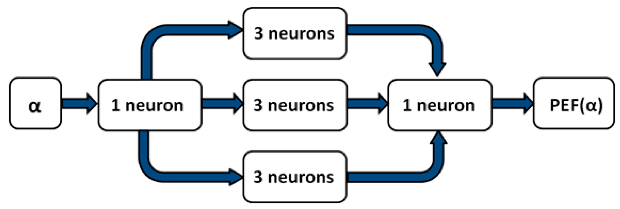
• α—angle in which the touch-trigger module is working,
• PE—probe error given as a result of PEF usage for considered angles.

The A and B angles were presented in Figure 2. They have their zero positions when the probe is oriented vertically. The α angle is dependent on the A and B angles. It is defined on the plane perpendicular to the probe when it is oriented using A and B angular positions, and has its zero indication in the direction in which the probe rotates along the A axis in the positive direction. The angle increases in the counterclockwise direction.

Depending on those three input parameters, the model provides the output value, which is the simulated value of the PE. The simulation is based on the Monte Carlo method and trilinear interpolation adapted for usage in polar systems. It uses the values of PE identified experimentally for selected A, B and α angles (experiments aimed at determining these values are presented in Section 2.2). The points determined using these angles for the chosen stylus used during measurements may be treated as nodes of the reference point grid. Let A_s, B_s and α_s denote the values of angles for which the simulation of errors has to be performed. A_s−1, B_s−1 and α_s−1 are the values of angles for the nearest node with angles lower than A_s, B_s and α_s, respectively, and A_s+1, B_s+1 and α_s+1 are the values of angles for the nearest node with corresponding angles higher than A_s, B_s and α_s. The values of PEs in nodes surrounding the point defined using A_s, B_s and α_s have to be used. In order to simulate the PE value for the point defined using A_s, B_s and α_s, the values of PEs in nodes surrounding this point have to be simulated using the Monte Carlo method. For all of the simulations presented here, the Monte Carlo method uses the scaled and shifted t-distributions with parameters ($\overline{x}$, s, ν), where $\overline{x}$ denotes the mean radial PE, s is the standard deviation associated with $\overline{x}$ and ν is the number of degrees of freedom. The parameters of these distributions are determined using the experiment presented in Section 2.2. Hence, the simulation should be performed for nodes (A_s−1, B_s−1, α_s−1), (A_s−1, B_s−1, α_s+1), (A_s−1, B_s+1, α_s−1), (A_s−1, B_s+1, α_s+1), (A_s+1, B_s−1, α_s−1), (A_s+1, B_s−1, α_s+1), (A_s+1, B_s+1, α_s−1) and (A_s+1, B_s+1, α_s+1). Then, a trilinear interpolation according to Formula (6) should be performed in order to obtain the PE value for the simulated point.

PEF(A_s, B_s, α_s) = ((A_s+1 − A_s)/(A_s+1 − A_s−1) × ((B_s+1 − B_s)/(B_s+1 − B_s−1) × P2 + (B_s − B_s−1)/(B_s+1 − B_s−1) × P4)) + ((A_s − A_s−1)/(A_s+1 − A_s−1) × ((B_s+1 − B_s)/(B_s+1 − B_s−1) × P1 + (B_s − B_s−1)/(B_s+1 − B_s−1) × P3))

(6)

where:

• P1 = (((α_s+1 − α_s)/(α_s+1 − α_s−1)) × PEF(A_s+1, B_s−1, α_s−1)) + (((α_s − α_s−1)/(α_s+1 − α_s−1)) × PEF(A_s+1, B_s−1, α_s+1))
• P2 = (((α_s+1 − α_s)/(α_s+1 − α_s−1)) × PEF(A_s−1, B_s−1, α_s−1)) + (((α_s − α_s−1)/(α_s+1 − α_s−1)) × PEF(A_s−1, B_s−1, α_s+1))
• P3 = (((α_s+1 − α_s)/(α_s+1 − α_s−1)) × PEF(A_s+1, B_s+1, α_s−1)) + (((α_s − α_s−1)/(α_s+1 − α_s−1)) × PEF(A_s+1, B_s+1, α_s+1))
• P4 = (((α_s+1 − α_s)/(α_s+1 − α_s−1)) × PEF(A_s−1, B_s+1, α_s−1)) + (((α_s − α_s−1)/(α_s+1 − α_s−1)) × PEF(A_s−1, B_s+1, α_s+1))

The presented model may serve two primary purposes. The first involves its use as part of virtual model of a five-axis coordinate system. In this application, it should be connected with one of the modules responsible for the simulation of the CMM's kinematic system errors (presented in [10,12,13,16]). For all of the points considered in a simulated measurement, the kinematic errors should first be simulated, and then the probe head errors should be simulated using the presented model. A single simulation of the probe head error for the considered point is done using the methodology presented above. For proper functioning of the virtual model, the simulation should be repeated n times, where n is the number of Monte Carlo trials set by the user or manufacturer of the virtual CMM software.

The second possible usage of the developed model is to utilize it for simulation and correction of probe head errors during the measurements performed in five-axis mode. A detailed description of this process is presented in Section 2.4.

2.2. Implementation Measurements

In order to gather the input data set for model, the reference ring was measured with different angular orientations of the probe head. The reference rings used during experiments were attached to a solid block which was installed in a swivel and tilting vise. A ring with a 20 mm diameter was chosen for the measurements, while other rings were used during datum definition and in further experiments (Section 3.3). In each ring arrangement, the standard was measured 15 times in 64 evenly distributed measured points. For the datum system definition, the CMM works in standard three-axis mode while all reference ring measurements were done using only rotational moves of the probe head. Therefore, the possible influences of machine kinematics are minimized. The positions were selected in a manner that allows covering the majority of the probe head working range. The orientation of the reference ring was changed together with the angular orientation of the probe. The utilized vise allows us to rotate the installed object around two perpendicular axes of revolution, and thus it is possible to set the ring so its axis will be oriented parallel to the stylus in A, B orientation. The authors decided to base the model on measurements carried out in 24 positions defined using B and A probe angles. Angle B changes at 60° in the range between −120° and 180°, while angle A changes at 30° in the range between 0° and 90°. Measurements for one of the described positions are presented in Figure 3.

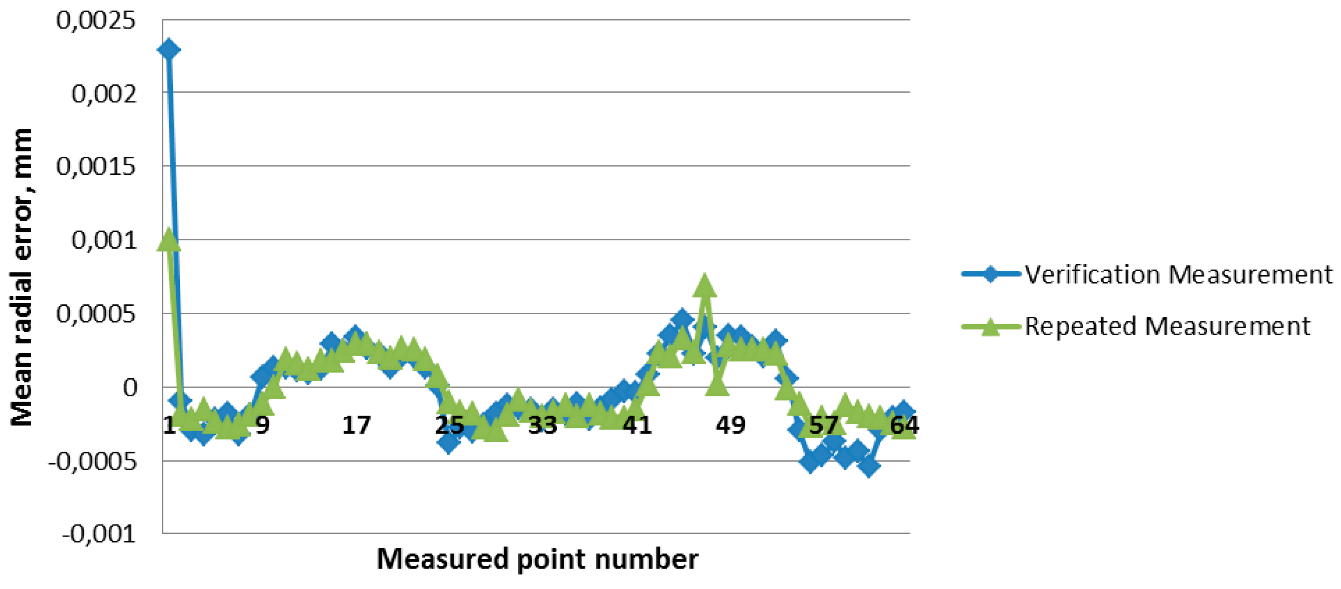
2.3. Verification Measurements

After the preparation measurements, the ring was measured in further positions to create the verifying data set. The 84 additional positions were selected with B changing at 20° between (−160°; 180°), and A changing at 15° between (0°, 90°). The same measuring procedure was used. The results obtained during these measurements are used to check the difference between the simulated values and the empirically gathered data. The authors assumed that the PE value may be considered as simulated correctly if it differs from the corresponding value obtained experimentally not more than ±3 * standard deviation assigned to the considered point.

2.4. Correction of Probe Head Errors Using the Developed Model

To perform a simulation and correction of probe head errors during the measurements performed in five-axis mode, the A, B and α angles of all points that were measured have to be recorded. Then the simulations according to the presented methodology have to be performed n times for all of these points. The mean from n simulated values is taken as the probe head error (PE) for the considered point (depending on α). To perform the correction of this error, the PE_x, PE_y and PE_z components have to be calculated using Equations (2)–(4). Then, the values of these components should be subtracted from the actual values of point coordinates x, y, z, giving the corrected point coordinates x_corr, y_corr and z_corr from Equations (7)–(9).

x_corr = x − PE_x

(7)

y_corr = y − PE_y

(8)

z_corr = z − PE_z

(9)

All measured features and relations should be calculated once again using the corrected point coordinates x_corr, y_corr and z_corr. In the presented research, the process of correction of the probe head errors was assisted by a script written in the Python programming language cooperating with macro prepared in Modus software. The raw measurement data including point coordinates, approach vectors and stylus orientation angles was sent to the Python script, which performed the correction of probe head errors and sent back corrected point coordinates to the metrological software, in which the calculation of measured features was done once again.

3. Results

Results presented in this section are the results of experiments described in Section 2. All experiments were performed at the Laboratory of Coordinate Metrology on a Zeiss WMM 850S machine (Carl Zeiss, Jena, Germany) equipped with a Renishaw PH20 probe head and a TP20 standard force module and a stylus with a 4 mm ball and a length of 10 mm. The machine is placed in an air-conditioned room with thermal stability at the level of 20 ± 0.5 °C. Modus metrological software was used on the machine.

3.1. Results of Identification of Errors

Figure 4 presents the results for a B angle equal to 120° and A changing in the range 0–90°.

The results of probe head error identification are used as an input data for the presented simulative model. They are given in tabular form. The example of such a table is presented in

Table 1. Example of input data for simulative model for A = 30° and B = −120°. A, B, α given in degrees; $\overline{x}$, s in mm.

A	B	α	$\overline{x}$	s	A	B	α	$\overline{x}$	s
30	−120	0.000	−0.00072	0.00048	30	−120	180.000	−0.00017	0.00016
30	−120	5.625	0.00007	0.00019	30	−120	185.625	−0.00034	0.00019
30	−120	11.250	0.00007	0.00020	30	−120	191.250	−0.00024	0.00020
30	−120	16.875	0.00015	0.00019	30	−120	196.875	−0.00034	0.00017
30	−120	22.500	0.00022	0.00013	30	−120	202.500	−0.00010	0.00019
30	−120	28.125	0.00029	0.00016	30	−120	208.125	0.00005	0.00029
30	−120	33.750	0.00015	0.00016	30	−120	213.750	0.00016	0.00027
30	−120	39.375	0.00010	0.00017	30	−120	219.375	0.00032	0.00019
30	−120	45.000	0.00020	0.00023	30	−120	225.000	0.00018	0.00019
30	−120	50.625	0.00019	0.00016	30	−120	230.625	0.00010	0.00012
30	−120	56.250	0.00029	0.00017	30	−120	236.250	0.00012	0.00018
30	−120	61.875	0.00009	0.00021	30	−120	241.875	0.00039	0.00022
30	−120	67.500	0.00010	0.00018	30	−120	247.500	0.00035	0.00020
30	−120	73.125	0.00012	0.00020	30	−120	253.125	0.00026	0.00016
30	−120	78.750	0.00012	0.00016	30	−120	258.750	0.00036	0.00015
30	−120	84.375	0.00016	0.00014	30	−120	264.375	0.00027	0.00019
30	−120	90.000	0.00014	0.00011	30	−120	270.000	0.00009	0.00014
30	−120	95.625	0.00004	0.00010	30	−120	275.625	0.00012	0.00020
30	−120	101.250	−0.00001	0.00023	30	−120	281.250	−0.00003	0.00018
30	−120	106.875	0.00000	0.00012	30	−120	286.875	0.00003	0.00018
30	−120	112.500	−0.00003	0.00015	30	−120	292.500	−0.00001	0.00024
30	−120	118.125	−0.00007	0.00013	30	−120	298.125	−0.00004	0.00016
30	−120	123.750	0.00019	0.00011	30	−120	303.750	−0.00037	0.00024
30	−120	129.375	0.00004	0.00017	30	−120	309.375	−0.00020	0.00018
30	−120	135.000	−0.00004	0.00017	30	−120	315.000	−0.00016	0.00014
30	−120	140.625	−0.00030	0.00019	30	−120	320.625	−0.00006	0.00018
30	−120	146.250	−0.00021	0.00016	30	−120	326.250	−0.00007	0.00013
30	−120	151.875	−0.00023	0.00016	30	−120	331.875	−0.00010	0.00014
30	−120	157.500	−0.00019	0.00017	30	−120	337.500	−0.00032	0.00013
30	−120	163.125	−0.00014	0.00021	30	−120	343.125	−0.00033	0.00015
30	−120	168.750	−0.00009	0.00021	30	−120	348.750	−0.00027	0.00015
30	−120	174.375	−0.00011	0.00011	30	−120	354.375	−0.00021	0.00016

.

The mean absolute radial error for all positions of the standard ring was equal to 0.0002 mm. The mean value of the standard deviation was equal to 0.0002 mm. The rest of the results of the error identification may be found in the supplementary materials added to this paper (Table S1).

The authors also repeated measurements of the ring in select positions to determine whether the probe error distributions retain their character. These measurements were carried out after the verification measurements to assess how the considerable exploitation of the probe head (the whole measuring procedure for one position consists of 960 measured points) affects the obtained results. Figure 5 presents the results of verification measurement for position B = 0°, A = 45° and the results obtained for repeated measurements in the same position. The measurements were repeated after measurements of 46 other positions. The results obtained for the checked positions show satisfactory consistency; therefore, it is justified to base the model on a data set obtained using the experiments described in Section 2.2.

3.2. Results of Model Verification

The verification of the model was done according to methodology presented in Section 2.3. The verification was done for 84 positions of the standard ring. Figure 6 and Figure 7 present the comparison between the results of the experimental probe head error identification and the simulation using the developed model for A = 75° and B = 80° (Figure 5) and A = −100° and B = 30° (Figure 6).

For the first position the mean absolute difference between the real values of the probe head errors (determined experimentally) and the simulated ones was equal to 0.0002 mm and for the second position 0.0001 mm. The authors assumed that the PE value may be considered as simulated correctly if it differs from the corresponding value obtained experimentally not more than ±3 × standard deviation assigned to the considered point. Out of 64 simulated values of PE for each position, 61 (95.31%) were properly simulated for the first position and 64 (100%) for the second position (according to assumption presented in Section 2.3).

3.3. Example of Probe Head Error Correction

The possibility of correcting probe head errors was presented on the example of measurements of the standard ring with a diameter of 34 mm. The values of diameter and roundness deviation were determined during the measurements. The ring was mounted in the plane perpendicular to the probe oriented using A = 43° and B = 91°.

Table 2. Results of roundness deviation measurements (given in mm) for standard ring with and without probe head errors correction.

Number of Points Used	Without Correction	With Correction	Calibration Certificate
64	0.0013	0.0010	0.0004
16	0.0012	0.0008	0.0004
8	0.0010	0.0005	0.0004

presents the results obtained during the real measurements without compensation of the probe head errors and after the compensation done using the methodology presented in Section 2.4. Results were compared with the data given on the calibration certificate of the ring.

4. Discussion

The primary conclusion of the presented experiments is that the developed simulation model allows for faithful reproduction of the error field for probe heads used in five-axis coordinate systems. In the case of the two presented positions used during verification measurements, the percentage of properly simulated error values was 95.31% and 100%, respectively. Such high numbers prove the effectiveness of the presented model and suggest its possible application as a module for probe head error simulation in virtual models of five-axis CMMs.

The developed model may also be helpful during the correction of probe head errors. As was shown in Table 2, the precision of the roundness deviation measurements has noticeably improved following the implementation of the correction using the methodology presented in Section 2.4. It should be noted that the effectiveness of probe head error correction is more pronounced in the case of a smaller number of measuring points used for the calculation of geometrical features. In this paper, example measurements were carried out on a circle, but the authors’ previous research suggests similar relationships in the case of other features. This phenomenon is connected with the averaging tendency of the least squares method, usually utilized for calculating features.

The results presented in Figure 5 indicate good stability of probe head error characteristics. It can be concluded from this that irrespective of the usage of the developed model, the initial measurements aimed at gathering input data for the model would not have to be repeated very frequently. The ideal interval for the re-identification of probe head errors should be investigated for different probe head types, but the authors suppose that it could be expressed in months.

As for future research directions, the most important goal is to develop a fully functional virtual model of a five-axis coordinate system. The research presented in this paper marks the first step in this direction. The simulative model discussed here should be connected to a model responsible for simulating kinematic system errors of the machine. Such a combined virtual model would reduce the time spent on the determination of the uncertainty of measurements performed on the five-axis coordinate system. Seeing as numerous systems of this type are presently used in industrial conditions, this would be likely to significantly reduce costs associated with quality control, and as a natural consequence, the total production costs would also drop down.

The model presented in this paper was checked for the measurements of regular rotary features for which the probes such as the one discussed here are usually applied in practice. In case of features such as cylinders, circles, spheres, cones, etc., the measurements may be easily performed using only the movements of the probe head, which significantly reduces their total time (in relation to the standard three-axis CMM). The measurements of more complicated shapes are also possible but the reduction of the measurement duration is not that meaningful as in the case of regular features. So it may be concluded that the model works properly for the majority of practical usages of the discussed probes. However, in the future, it will be advisable to also include in it the possibility of simulating the measurements of more complicated geometries, when the stylus has to move on complex trajectories and the α angle cannot be easily defined on the plane perpendicular to the probe when it is oriented using A and B angular positions.

The next important possibility of improving the presented model is to reduce the number of orientations and points used during identification measurements. It should be possible to minimize their number in a way that simultaneously reduces the time needed for model implementation, and provides faithful reproduction of a real field of probe head errors.

References

1. Kunzmann, H.; Pfeifer, T.; Schmitt, R.; Schwenke, H.; Weckenmann, A. Productive metrology-adding value to manufacture. CIRP Ann. Manuf. Technol. 2005, 54, 691–704. [Google Scholar] [CrossRef]
2. Caja, J.; Gomez, E.; Maresca, P. Optical measuring equipments. Part I: Calibration model and uncertainty estimation. Precis. Eng. 2015, 40, 298–304. [Google Scholar] [CrossRef]
3. Asano, Y.; Furutani, R.; Ozaki, M. Verification of interim check method of CMM. Int. J. Autom. Technol. 2011, 5, 115–119. [Google Scholar]
4. Cuesta, E.; Alvarez, B.; Sanchez-Lasheras, F.; Gonzalez-Madruga, D. A statistical approach to prediction of the CMM drift behaviour using a calibrated mechanical artefact. Metrol. Meas. Syst. 2015, 22, 417–428. [Google Scholar] [CrossRef]
5. Takamasu, K.; Takahashi, S.; Abbe, M.; Furutani, R. Uncertainty estimation for coordinate metrology with effects of calibration and form deviation in strategy of measurement. Meas. Sci. Technol. 2008, 19. [Google Scholar] [CrossRef]
6. International Organization for Standardization. ISO 15530-3:2011—Geometrical Product Specifications (GPS)—Coordinate Measuring Machines (CMM): Technique for Determining the Uncertainty of Measurement—Part 3: Use of Calibrated Workpieces or Measurement Standards; ISO: Geneva, Switzerland, 2011. [Google Scholar]
7. Weckenmann, A.; Lorz, J. Monitoring coordinate measuring machines by calibrated parts. J. Phys. Conf. Ser. 2005, 13, 190–193. [Google Scholar] [CrossRef]
8. Sato, O.; Osawa, S.; Kondo, Y.; Komori, M.; Takatsuji, T. Calibration and uncertainty evaluation of single pitch deviation by multiple-measurement technique. Precis. Eng. 2010, 34, 156–163. [Google Scholar] [CrossRef]
9. Osawa, S.; Busch, K.; Franke, M.; Schwenke, H. Multiple orientation technique for the calibration of cylindrical workpieces on CMMs. Precis. Eng. 2005, 29, 56–64. [Google Scholar] [CrossRef]
10. Trapet, E.; Franke, M.; Hartig, F.; Schwenke, H.; Wadele, F.; Cox, M.; Forbers, A.; Delbressine, F.; Schnellkens, P.; Trenk, M.; et al. Traceability of Coordinate Measuring Machines According to the Method of the Virtual Measuring Machine; PTB: Braunschweig, Germany, 1999. [Google Scholar]
11. Schwenke, H.; Siebert, B.R.L.; Wäldele, F.; Kunzmann, H. Assessment of uncertainties in dimensional metrology by Monte Carlo simulation: Proposal of a modular and visual software. CIRP Ann. Manuf. Technol. 2000, 49, 395–398. [Google Scholar] [CrossRef]
12. Wilhelm, R.G.; Hocken, R.; Schwenke, H. Task specific uncertainty in coordinate measurement. CIRP Ann. Manuf. Technol. 2001, 50, 553–563. [Google Scholar] [CrossRef]
13. Sładek, J.; Gąska, A. Evaluation of coordinate measurement uncertainty with use of virtual machine model based on Monte Carlo method. Measurement 2012, 45, 1564–1575. [Google Scholar] [CrossRef]
14. Aggogeri, F.; Barbato, G.; Barini, E.M.; Genta, G.; Levi, R. Measurement uncertainty assessment of coordinate measuring machines by simulation and planned experimentation. CIRP J. Manuf. Sci. Technol. 2011, 4, 51–56. [Google Scholar] [CrossRef] [Green Version]
15. Giusca, C.L.; Leach, R.K.; Forbes, A.B. A virtual machine-based uncertainty evaluation for a traceable areal surface texture measuring instrument. Measurement 2011, 44, 988–993. [Google Scholar] [CrossRef]
16. Sładek, J. Coordinate Metrology: Accuracy of Systems and Measurements; Springer: Berlin, Germany, 2016. [Google Scholar]
17. Maresca, P.; Gomez, E.; Caja, J.; Barajas, C. Virtual environment for the simulation of a horizontal coordinate measuring machine in the teaching of dimensional metrology. Procedia Eng. 2013, 63, 234–242. [Google Scholar] [CrossRef]
18. Ostrowska, K.; Gąska, A.; Sładek, J. Determining the uncertainty of measurement with the use of a Virtual Coordinate Measuring Arm. Int. J. Adv. Manuf. Technol. 2014, 71, 529–537. [Google Scholar] [CrossRef]
19. Cuesta, E.; Talenti, A.; Patino, H.; Gonzalez-Madruga, D.; Martínez-Pellitero, S. Sensor prototype to evaluate the contact force in measuring with coordinate measuring arms. Sensors 2015, 15, 13242–13257. [Google Scholar] [CrossRef] [PubMed]
20. Nafi, A.; Mayer, J.R.R.; Wozniak, A. Novel CMM-based implementation of the multi-step method for the separation of machine and probe errors. Precis. Eng. 2011, 35, 318–328. [Google Scholar] [CrossRef]
21. Gąska, A.; Krawczyk, M.; Kupiec, R.; Ostrowska, K.; Gąska, P.; Sładek, J. Modeling of the residual kinematic errors of coordinate measuring machines using Laser Tracer system. Int. J. Adv. Manuf. Technol. 2014, 73, 497–507. [Google Scholar] [CrossRef]
22. Dobosz, M.; Woźniak, A. CMM touch trigger probes testing using a reference axis. Precis. Eng. 2005, 29, 281–289. [Google Scholar] [CrossRef]
23. Gąska, A.; Harmatys, W.; Gąska, P.; Gruza, M.; Mathia, T.; Sładek, J. Optimization of probe head errors model used in Virtual CMM systems. In Proceedings of the 11th International Conference on Laser Metrology and Machine Performance (LAMDAMAP) 2015, Huddersfield, UK, 17–18 March 2015; Blunt, L., Hansen, H.N., Eds.; euspen: Cranfield, UK, 2015. [Google Scholar]
Figure 1. Construction of the neural network used for probe error modeling. α: probe deflection angle; PEF: Probe Error Function.
Applsci 06 00144 g001
Figure 2. Articulated probe head used in five-axis coordinate systems with revolution axes marked. A: rotation angle along the horizontal axis of the probe head; B: rotation angle along the vertical axis of the probe head.
Applsci 06 00144 g002
Figure 3. Measurements of standard ring in one of the selected positions.
Applsci 06 00144 g003
Figure 4. Results of identification of errors for a B angle equal to 120° and A changing in the range 0–90°. All angles given in degrees and errors in mm.
Applsci 06 00144 g004
Figure 5. Results of mean Probing Error (PE) values obtained for the chosen position during verification measurements and measurements repeated after a relatively long time of probe head functioning.
Applsci 06 00144 g005
Figure 6. Comparison between results of experimental probe head errors identification and simulation using developed model for A = 75 and B = 80.
Applsci 06 00144 g006
Figure 7. Comparison between results of experimental probe head errors identification and simulation using developed model for A = −100 and B = 30.
Applsci 06 00144 g007