Effect of Islanding and Telecontrolled Switches on Distribution System Reliability Considering Load and Green-Energy Fluctuations

Abstract

To improve electrical distribution network reliability, some portions of the network could operate in autonomous mode, provided that the related technical issues are addressed. More specifically, when there is not a path from those portions to the primary substation due to a fault in the network, such portions could be disconnected from the main network and supplied by local generation only. Such a mode of operation is known as “intentional islanding” and its effectiveness, in terms of adequacy, depends on the ability of the local generation to meet the island’s load. In fact, the ratio between the available local generation and load demand can frequently change during islanding due to load variations and, especially, due to the strongly irregular behavior of the primary energy sources of renewable generators. This paper proposes an analytical formulation to assess local generation adequacy during intentional islanding, accounting for the aforementioned variations. More specifically, the fluctuations of load and green-energy generators during islanding are modeled by means of Markov chains, whose output quantities are encompassed in the proposed analytical formulation. Such a formulation is used by the analytical equations of load points’ outage rate and duration. The evaluation of the reliability indices accounts for a protection scheme based on an appropriate communication infrastructure. Therefore, a brief overview on the telecommunications technologies has been presented with reference to their suitability for the specific application. In particular, distribution network safety issues have been considered as the main concern. The results show that neglecting load and generation fluctuations leads to a strong overestimation of the ability of distributed generators to meet the island load. Through a case study it is observed that the error on the load point outage rate is greater than the one affecting the outage duration.

1. Introduction

The deregulation of the electricity market and the introduction by national authorities of reward/penalty mechanisms are driving distribution network operators (DNOs) to improve the reliability performance of distribution systems [1]. The DNOs can employ different strategies to improve the reliability performance of the distribution networks: executing network maintenance actions to prevent fault events [2]; reallocating or installing additional switches along the distribution network [3]; introducing telecontrol and automation systems [4]; adopting new network management paradigms, such as operating some portions of the network in island mode when a fault occurs [5], i.e., disconnecting them from the main network and supplying by local generation; and so on.

Environmental and long-term primary energy resources provision concerns are driving towards an increasingly diffusion of renewable energy technologies [6]. In Europe the 20-20-20 2020 climate & energy package (aiming to meet 20% of energy needs by means of renewable sources and reduce both energy consumption and pollutant emissions by 20% by 2020 [7]) has led many countries to introduce new policies that provide incentives for using renewable energy sources and maximizing energy efficiency.

Therefore, considering that the distribution system has been planned and managed by means of procedures dating back to the 1960s, DNOs have to face a new challenging scenario. The Smart Grid (SG) paradigm [8] is the key to addressing these issues; indeed, it is expected that SG will exploit communication and automation systems to minimize the impact of renewable-based Distributed Generators (DGs) on the distribution network. On the other hand, SG can convert DGs into a resource by managing them [9]. In fact, from an SG perspective the possibility of meeting the load of intentional islands by means of local generation combined with the introduction of telecontrolled switches is desirable from a reliability point of view [4].

The use of telecontrolled sectionalizers enables the DNO to quickly restore the portion of the network not affected by the fault, thereby improving the average annual outage duration per customer. In recent years, "Global System for Mobile communications" (GSM) technology has been adopted and telecontrolled sectionalizers have been installed in order to meet the target imposed by the authorities [10]. On the other hand, reducing the average annual outage rate per customer requires installing telecontrolled circuit breakers (CBs). In this paper, delayed operation of the CBs is considered to perform logic selectivity. In other words, when a fault occurs, a centralized control system receives information about the fault current directions from the CBs that detected the fault. These CBs do not open instantaneously (since a delayed tripping time is adopted) but they send such information to the control system. After that, according to the logic selectivity, the CBs closest to the fault receive an opening authorization while the others receive a command that forces them to remain closed in order to leave the smallest portion (faulted zone) of the network unsupplied (a CB is considered the “closest” to the fault if there is not any CB between itself and the fault). For safety reasons, a CB has to be opened when it detects the fault but does not receive any communication within its delayed operation time. More specifically, the network protected by the CB could be damaged due to a fault current persisting beyond the physically admissible time; hence the delay time has to be properly chosen and the CB is automatically opened by local control when it does not receive a command that forces it to remain closed. Therefore, smart communications subsystems (SCSs) that enable to open the closest CBs while keeping the others closed with a reasonable time delay are investigated in the paper. Although a lot of work has been done in the past regarding the choice of an appropriate technology for an SCS [11], the suitability of different solutions for information exchange when a fault occurs in the distribution network has rarely been investigated.

The most used adequacy indices are the Loss of Load Expectation (LOLE), the Loss of Load Probability (LOLP), and the Loss of Energy Expectation (LOEE) [12]. Such indices could be adopted to evaluate the adequacy of local DGs supplying an island, but they do not account for load curtailment policies since they consider load shedding only [13]. In [5] a new adequacy index, called Probability of Adequacy (PoA), has been proposed to overcome this limitation. The main merit of the PoA assessment approach is its ability to account for the probability that a given load and a given generation level occur when a network portion intentionally passes from the connected to the island mode of operation, as well as considering load shedding and/or curtailment policies. On the other hand, this approach neglects the variations of load and generation that usually occur when the island mode is maintained for several hours, and, consequently overestimates the ability of islanding to improve distribution system reliability. This aspect is crucial especially when renewable DGs are considered, due to the fluctuating behavior of their primary (green) energy sources (wind, sun) [14].

The present work proposes an efficient computational approach that is able to overcome the limitation of the previous ones and also account for load and generation correlations, thus obtaining a very accurate measure of the reliability improvement that can be achieved thanks to islanding in distribution networks where telecontrolled CBs as well as telecontrolled and manual sectionalizers are installed.

In order to calculate distribution network reliability, the analytical equations of load point outage rate and duration that account for a protection scheme based on telecontrolled switches [4] are combined with the formulation proposed for adequacy computation. Such a formulation uses a Markov chain for modeling the ratio between load and generation. Thanks to its properties of capturing both first- and second-order statistics [15], the proposed Markov chain is also able to represent the fluctuation during islanding of load and green-energy generators and accounting for correlations.

It is to be noted that supplying as many customers as possible each time a change occurs in the load and/or generation level is the best strategy in terms of average outage duration but it is the worst in terms of average outage frequency, since some customers can be repeatedly left unsupplied and reconnected many times during islanding. Therefore, the proposed formulation for adequacy computation does not consider resupplying those customers previously left unsupplied during islanding. Obviously, those customers will be reconnected to the network after the fault is repaired.

The rest of the paper is structured as follows. In Section 2 the background is reported for the sake of completeness. A brief overview of telecommunications technologies is presented in Section 3, with reference to their suitability for the considered protection scheme. In Section 4, the proposed model approach is described, by means of Markov chains, the behavior of loads, and distributed generators. Such models are applied in Section 5 to provide the proposed indices as a measure of the adequacy of island generation. A case study is presented in Section 6 and the conclusions in Section 7. Finally, the nomenclature is reported in the "Abbreviations" section.

2. Background

2.1. Annual Model of Loads and Distributed Generators

The annual load model related to a load point (LP) i is usually obtained by means of the historical power demand of the customers connected to the LP. It is represented by considering several power demand levels with their occurrence probability, as reported in

Table 1. Example of annual load model for a load point i with five levels ($N_i^D=5$).

Level (l)	Power Demand (% of Annual Peak)	Probability $\left({\mathsf{\pi }}_{i,l}^{(D)}\right)$
1	20	0.17
2	40	0.22
3	60	0.26
4	80	0.24
5	100	0.11

. Similarly, the annual generation model of a renewable DG (RDG) r is obtained by the historical generation data. The model can also be obtained by computing the potential power output by properly combining historical meteorological data and the hardware unavailability [16,17,18] (that is the forced outage rate, usually known as FOR [19]).

Table 2. Example of annual generation model for a renewable distributed generator r with five levels ($N_r^G=5$).

Level (l)	Power Output (% of Rated Power)	Probability $\left({\mathsf{\pi }}_{r,l}^{(RG)}\right)$
1	20	0.36
2	40	0.28
3	60	0.20
4	80	0.11
5	100	0.05

shows an example of annual generation model for a renewable generator. Finally,

Table 3. Example of annual generation model for a conventional distributed generator c, considering its forced outage rate (FOR).

Level (l)	Power Output (% of Rated Power)	Probability $\left({\mathsf{\pi }}_{c,l}^{(CG)}\right)$
1	0	FOR
2	100	1-FOR

reports the annual model of a conventional DG (CDG, e.g. diesel), whose output does not depend on a fluctuating primary energy source.

2.2. Analytical Assessment of the Probability of Adequacy (PoA)

The load and generation models were combined in [5] to assess the PoA of an island j. Assuming that there are $L_j$ loads, $R_j$ RDGs, and $C_j$ CDGs in the considered island, the number $M_j$ of combinations depends on the number of levels in each load model, as well as in the generation model of each DG. Therefore, $M_j$ is equal to the number of working points at which the island can operate, that is:

$$M_j={\displaystyle \prod _{i=1}^{L_j}}{N}_i^D\cdot {\displaystyle \prod _{r=1}^{R_j}}{N}_r^G\cdot 2^{C_j}.$$

(1)

For a given combination m, the total available local generation $G_{j,m}^E$ is compared with the whole power demand $D_{j,m}^E$ of the island’s LPs to assess the load fraction that can be supplied by the island’s DGs when combination m occurs. Weighting such a fraction by the occurrence probability, the related PoA (ρ_A,j) is computed as follows:

$${\mathsf{\rho }}_{A,j}={\displaystyle \sum _{m=1}^{M_j}R{}_{j,m}\cdot {\mathsf{\pi }}_m^{\left(R_j\right)}},$$

(2)

where:

$$R_{j,m}=\min \left(1;\frac{G_{j,m}^E}{D_{j,m}^E}\right)$$

(3)

and ${\mathsf{\pi }}_m^{\left(R_j\right)}$ is the occurrence probability of the m-th combination.

This approach neglects the second-order statistics of the time variations of load and generation that usually occur when the island mode persists for some hours. In other words, the previous approach considers that R_j,m does not change during the interval in which the portion of the network works in autonomous mode. To this purpose, in Section 4 a Markov chain will be introduced to model the time evolution of R_j,m, and its dependence on the time-variant behavior of both load and generation processes.

2.3. Analytical Evaluation of Distribution System Reliability Accounting for Islanding and Telecontrolled Switches

In the following, the term node will indicate either a point (bus) in the medium-voltage network where customers and/or generators are connected, or a switching substation. A node is an LP if at least one customer is connected to it. The electrical equipment connecting two nodes will be indicated as a branch. The branches are numbered sequentially and each node takes the number of the upstream branch, with reference to the primary substation (PS) position, as shown in Figure 1. Moreover, it is assumed that a sectionalizer is always installed where a circuit breaker is placed (in the following a CB and sectionalizer taken as a whole are referred to as a CBS). The switches placed in the network are CBSs and sectionalizers only, and a potential island is related to each switch. The CBS operations are delayed in order to telecontrol them, so as to enable a logic-selectivity-based protection scheme. Also, some sectionalizers are telecontrolled to enable faster restoration of the network portions outside of the faulted zone. The distribution management system (DMS) receives information from the switches detecting the fault and, firstly, sends an opening authorization to some CBSs while it forces the others to remain closed; then the DMS performs the restoration procedures, operating the telecontrolled sectionalizers.

The effect of a faulted branch on a LP depends on the LP location, the location of the faulted branch, the type of the switches, and the installation point. Moreover, the effect also depends on the LP power demand and DG type, the capacity, and the location, when islanding is permitted. The PoA is a measure of this effect. More specifically, many different “scenarios” can be accounted for by analyzing the potential effects [4]. For the sake of completeness, Appendix A reports the formulas to be used to assess outage rate (λ_i,k) and duration (U_i,k) at LP i when a fault occurs in branch k, for all possible scenarios. Further details can be found in [4].

3. Comparison of Telecommunications Technologies to Support the Protection Scheme

One of the key elements for a correct and efficient management of a SG is the SCS. A lot of work has been done in the past regarding the technological choices for a SCS, but the suitability of different solutions for information exchange when a fault occurs in the distribution network to operate the switches, especially the CBs, has rarely been investigated. To this aim, in this section some telecommunications technologies of the SCS are reviewed and compared to investigate their suitability for implementing the considered protection scheme. More specifically, these technologies are evaluated in terms of their ability to enable CBs opening with a reasonable delay, since safety issues are the main concerns to be addressed.

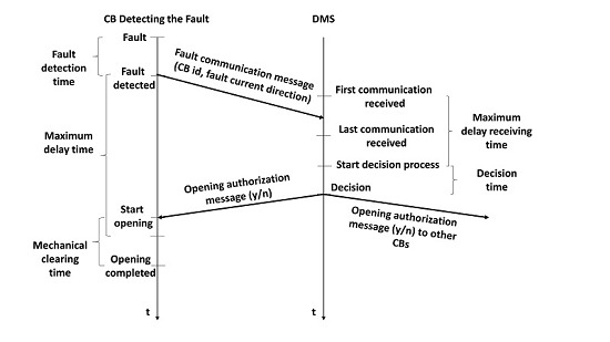
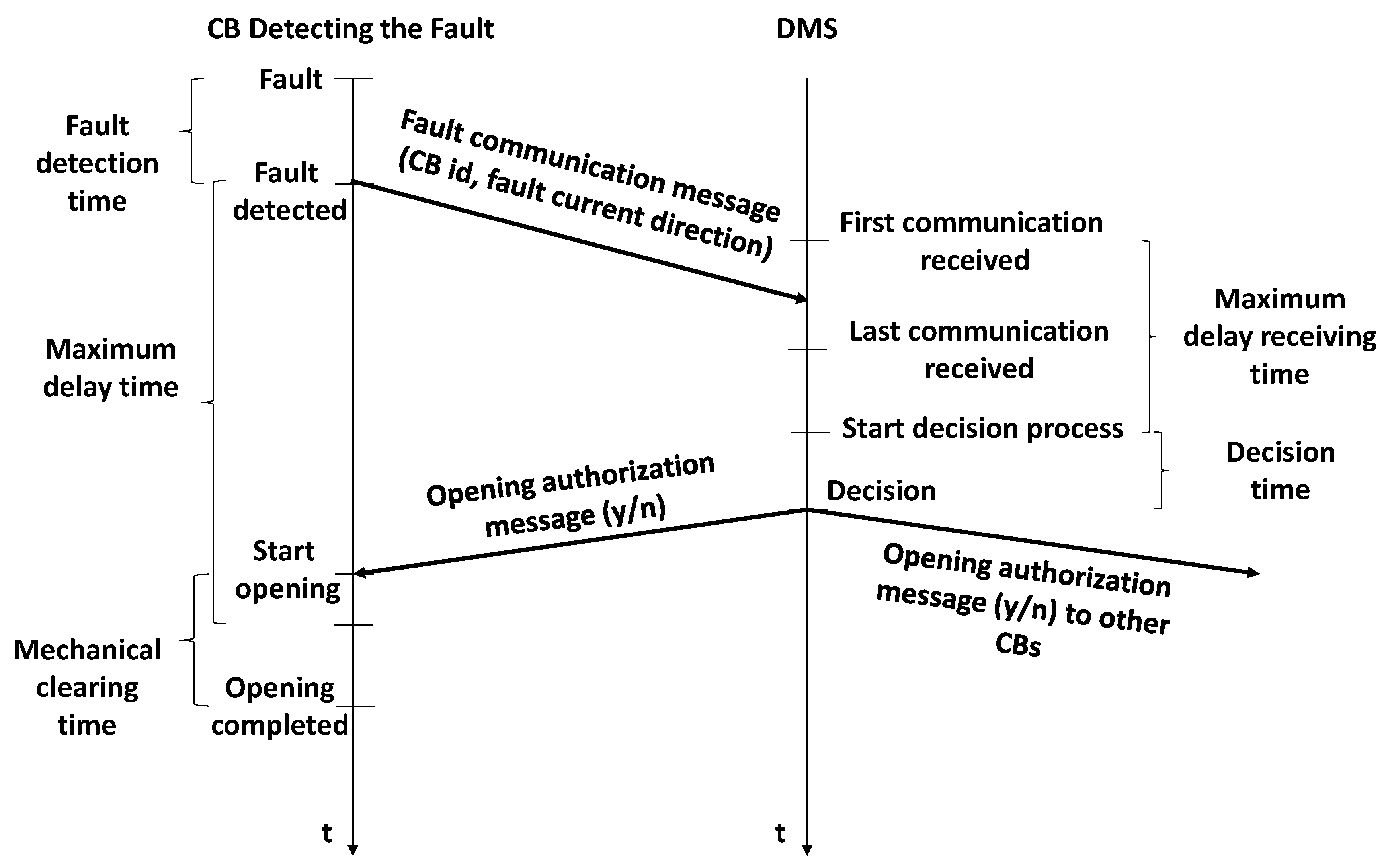
Figure 2 shows the time evolution of the fault clearing process related to a CB detecting a fault, highlighting the maximum delay time for safety reasons (typical values are around 100 ms), and the time needed to exchange messages between the above CB and the DMS located at the PS. If the message exchanging time duration is greater than the maximum delay time, the CB will open even when not necessary.

Therefore, the choice of telecommunications technology is a challenge because it depends on many elements, including the quality of service requirements characterizing the SG, the telecommunications network infrastructures that are already available in proximity of each node of the SG, and the presence of factors that can justify investments in network facilities but that are external to our specific goal of supporting SG management in cases of faults.

The following considerations should be taken into account:

(a)

the best technological solution for a distribution network located in an urban area could be poor, unfeasible or totally unavailable for a network that is located in a rural area;

(b)

the distance between a switch and the PS could vary from less than one kilometer up to some tens of kilometers;

(c)

the distance between two nodes connected to each other can also be very different (from some tens of meters up to a few kilometers), and a direct wireless connection can be obstructed by buildings or natural barriers placed between them;

(d)

a telecommunications technology could be already installed for data transmissions during normal service conditions;

(e)

two nodes can be connected by an overhead (plain conductor or in cable) or underground (conductor in cable) line; in the first case the application of the powerline technology discussed below may not be reliable because the electrical line is exposed to highly variable conditions; and

(f)

a node could be a pole-mounted substation, a kiosk substation (metallic prefabricated, masonry, or reinforced concrete), or a vault substation.

With all this in mind, let us now compare the main technological solutions that can be generally applied to a SG, evaluating their appropriateness to the considered case, which is characterized by the peculiarities described above. Let us consider that, for our purposes, the main target of the SCS is to guarantee reliable point-to-point communication channel between each switch detecting the fault and the DMS. Moreover, for security reasons, this connection must respect a requirement in terms of end-to-end delay on the above point-to-point channel when the switch is a CB. In addition, different technological solutions can be adopted in the same SCS according to the specific situation of each node.

The first choice to be made is whether to use wireless or wired links. Among wireless technologies, one of the most widely recognized choices to support an SG is the wireless mesh network (WMN) [20], which is a communication network made up of wireless nodes organized in a mesh topology. Thanks to the presence of redundant paths, it is able to guarantee a high data rate, high communication reliability, and automatic network connectivity against potential problems, e.g., wireless node failures and path failures. However, these peculiarities, which are very important for managing SGs characterized by a high grade of connectivity and working in normal states, are not useful in our case. On the contrary, due to the presence of multi-hop communications through wireless links, typically based on the standards IEEE 802.11 and IEEE 802.16, the end-to-end delay caused by using an WMN can reach values a lot higher than the aforementioned maximum accepted values of 100 ms in the specific case considered in this paper [21,22,23]. Moreover, if the cheaper IEEE 802.11 is used to realize single-hop links, the number of consecutive hops can be high because of the limited range of coverage of each link (a few hundreds of meters) and the distance between each switch (CBS, sectionalizer) and the DMS installed at the PS. Consequently, besides unacceptable delays, this causes high vulnerability to failure. This problem could be overcome by the more recent standard version IEEE 802.11y, which allows one to transmit the signal up to 5 km at a rate of 54 Mbps but requires a licensed frequency band of 3.7 GHz, very high transmission power, and a specially designed antenna—conditions that often make it unfeasible.

The other wireless technology that allows major coverage and higher data rate is IEEE 802.16. It allows high data rates on distances of some kilometers, but requires Line Of Sight (LOS) between transmitting and receiving stations. This can be easily achieved in rural areas, while it is a problem in urban areas.

Similar considerations hold for microwave and free-space optical communications, both suitable for point-to-point communications. Microwave communications allow use of conveniently sized directional antennas to obtain transmissions at high bandwidths. Free-space optical communication, on the other hand, is a communication technology that uses light propagation in free space to transmit point-to-point data at high bit rates with low bit error rates. However, due to the LOS requirement, the transmission quality achieved with them is greatly affected by obstacles (e.g., buildings and hills) and environmental constraints (e.g., rain fade), making them unsuitable during particular weather conditions and not applicable in urban areas. Instead, they are very useful in rural areas, where using other wireless or wired technologies is costly or even impossible.

Other wireless technologies like Bluetooth, ZigBee, WirelessHART, and ISA100.11a, all based on the IEEE 802.15.4 protocol stack, although strongly applied at the edge of SGs in the customer home networks, are not applicable in our context for their very short range of coverage. In addition, Bluetooth has a very high network joining time, around 3 s, compared to 30 ms for ZigBee.

On the other hand, satellite channels, widely considered as backup channels in case of disaster [24] to maintain the normal state of an SG, cannot be considered when a fault occurs because of their unacceptable latency as compared with the maximum acceptable delay of 100 ms.

Finally, another wireless solution is given by the communications channels based on cellular communications, that is, the short message system and the more complex Wireless Wide Area Networks [25]. The first technique is widely used today to execute restoration procedures by means of telecontrolled sectionalizers. On the other hand, the very huge end-to-end delays, on the order of some seconds [26], limit its application to CBs. The second technology is realized as networks of cellular channels following the evolution of the cellular network standards, starting from the first version of General Packet Radio Service (GPRS) up to the modern 4G. Since all the cellular technologies deployed up to now are characterized by round-trip delays ranging between 800 ms and 8 s (in some bad cases) [27], they cannot be applied to the considered case where the fault messages have to be delivered within 100 ms.

An alternative solution to wireless links is given by wired technologies, mainly dominated by fiber-optic communications and power-line communications (PLC). Both technologies are able to guarantee very low end-to-end delays, given that signals propagate with a speed comparable to the speed of light. Since in our application the amount of data to be transmitted is very small, the end-to-end latency, that is the sum of the transmission delay and the propagation delay, is strongly acceptable and on the order of a few msec.

Nevertheless, the main advantages of fiber-optic communications, i.e., their very high transmission rates, very low delays, and immunity to electromagnetic and radio interference (matters that are very important for high-voltage operating environments like the one considered in this paper), are not well balanced by their expensive installation costs, also taking into account the large amount of spare capacity. Therefore their application is justified in our scenario if the energy provider installs them for other goals, for example a leasing agreement with telco operators, or to support the normal state of an SG populated with a huge number of devices.

The other wired technology that is very powerful for the SCS of an SG is PLC [28]. It is a technology for carrying data on the same conductors of the electrical grid, and for this reason it has deployment costs comparable to wireless technologies since the lines are already there. This technology, already widely applied in low-voltage distribution grids (close to homes), is well suited for smart metering infrastructure and enables communications between electric vehicles and a power grid (narrowband PLC), as well as transferring data seamlessly from SG controllers to home networks and vice versa. However, its application to manage the clearing process in the distribution networks is very complex because it needs to carry data through the electrical line when it is open.

The application of the PLC technologies is still possible but requires some deployment expedient to also maintain connectivity in the presence of a fault in the distribution network. A way to apply it is to use a two-step double technology. More specifically, if the fault is on one phase of a three-phase conductor, the PLC channel can work on the two other phases to communicate the fault to the DMS in order to operate the CBs. Once the CBs are opened, the following communications cannot be realized with PLC because the conductors are open. Then another technology (e.g., GSM) can be used for the telecontrolled sectionalizers because the end-to-end delay is not yet a stringent constraint for safety purposes, although the portions of the network outside of the faulty zone must be restored as soon as possible considering that the DNO is affected by the reward/penalty mechanisms. On the other hand, such a two-step double technology fails when a three-phase fault occurs and consequently cannot be adopted to implement the considered protection scheme.

4. Markov Models for Adequacy Evaluation

In this section the models of an equivalent load and an equivalent generator in an island are defined. These models are then combined to obtain R_j,m, as calculated in Equation (3), in order to derive the PoA more accurately, that is accounting for the time variations of load and generation that usually occur when the island mode is maintained for some hours.

4.1. Markov Model of the Island’s Load

Considering an island j with $L_j$ LPs, the model of an equivalent load is obtained by combining, and then quantizing, the historical data for power demand at each LP. To this end, the sampling start time of the historical data is indicated as $T_0$, and the sampling period as $\Delta T$. The equivalent load before quantization, $D_j^{E,BQ}(p)$, is the overall power demand in the island j at the time slot p, and is calculated as:

$$D_j^{E,BQ}(p)={\displaystyle \sum _{i=1}^{{}_{L_j}}{D}_i(p)},$$

(4)

where $D_i(p)$ is the power absorbed at the LP $i$ at the generic sampling instant $T_0+p\Delta T$ (that is, at slot p). Such an approach enables one to account for correlations (e.g., hourly, seasonal, and so on) among power demands.

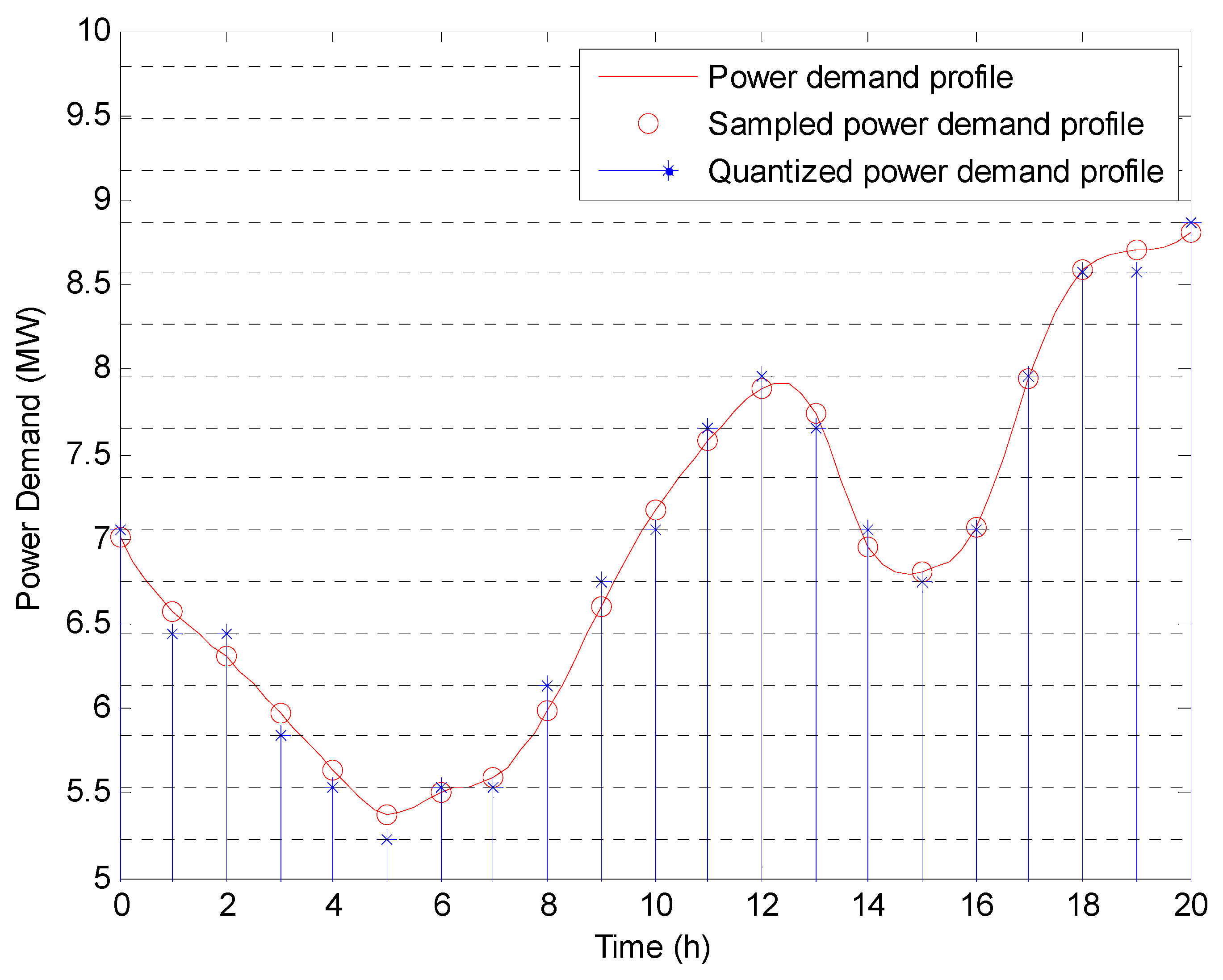
Since the equivalent load exhibits continuous values, it is discretized through a uniform quantization, as shown in Figure 3. Let $D_j^E(p)$ be the quantized process of the power demand in the island. By indicating the quantization interval for the island j as $\Delta L_j$, the number of quantization levels used for the generic island j as $N_{D,j}$, and the quantized values as $d_j^l$, with $l=1,2,\mathrm{...},N_{D,j}$, the sampled power demand assumes the value $d_j^l$ if:

$$D_j^{E,BQ}(p)\in \left[d_j^l-\frac{\Delta L_j}{2},d_j^l+\frac{\Delta L_j}{2}\right[.$$

(5)

In order to determine the model of the equivalent load, it is necessary to obtain the $N_{D,j}\times N_{D,j}$ transition probabilities matrix $P^{(D_j)}$. Its generic element is defined as the probability that $D_j^E(p)$ moves from the level $\mathsf{\alpha }$ to the level $\mathsf{\beta }$ in the transition from the time slot p to the time slot $p+1$, that is:

$$P_{\left[\mathsf{\alpha },\mathsf{\beta }\right]}^{(D_j)}=\text{Prob}{\left\{D_j^E(p+1)=d_j^{\mathsf{\beta }}|D_j^E(p)=d_j^{\mathsf{\alpha }}\right\}}^{}.$$

(6)

From the historical data, the probability in Equation (6) can be derived as follows:

$$P_{[\mathsf{\alpha },\mathsf{\beta }]}^{(D_j)}=\frac{v_{\mathsf{\alpha }->\mathsf{\beta }}^{(D_j)}}{{\displaystyle \sum _{{}^{}\mathsf{\gamma }=1^{}}^{N_{D,j}}{v}_{\mathsf{\alpha }->\mathsf{\gamma }}^{(D_j)}}}.$$

(7)

where ${\mathsf{\nu }}_{\mathsf{\alpha }\to \mathsf{\beta }}^{(D_j)}$ is the number of transitions from the level $\mathsf{\alpha }$ to the level $\mathsf{\beta }$ in the time period used to estimate the above probability.

4.2. Markov Model of the Island’s Generation

The method described above can also be applied to the renewable generators belonging to the island j. By indicating the process related to the aggregated renewable generation (obtained by firstly summing the concurrent powers generated by the DGs in the island, and then by quantizing the equivalent power) as $R{G}_j^E(p)$, a quantized value as $r{g}_j^l$, and the number of levels used to quantize this process as $N_{RG,j}$, a $N_{RG,j}\times N_{RG,j}$ transition probability matrix, $P^{(R{G}_j)}$, can be derived as in Equation (7). Such an approach enables us to account for power output correlations (e.g., hourly, seasonal, and so on).

A up-down model is considered for conventional generators [12]. For the generic CDG c, a $2\times 2$ transition matrix $P^{(CG,c)}$ fully describes its behavior. The CDGs belonging to the same island can be combined to obtain an equivalent model of the conventional generators. Through the Kronecker product of all the $P^{(CG,c)}$ matrices [29], a $2^{C_j}\times 2^{C_j}$ transition probability matrix, $P^{(C{G}_j)}$, is obtained, with $C_j$ being the number of CDGs in island j. As an example, the following matrix has been used to model the generic CDG c in the numerical results section:

$$P^{(CG,c)}=\left[\begin{array}{cc}9.722\cdot {10}^{-1}& 2.778\cdot {10}^{-2}\\ 2.296\cdot {10}^{-4}& 9.998\cdot {10}^{-1}\end{array}\right].$$

(8)

Therefore, the transition probability matrix of the aggregate of two CDGs is obtained as the Kronecker product of two matrices, both equal to $P^{(CG,c)}$:

$$P^{(C{G}_j)}=\left[\begin{array}{cccc}9.452\cdot {10}^{-1}& 2.701\cdot {10}^{-2}& 2.701\cdot {10}^{-2}& 7.716\cdot {10}^{-4}\\ 2.232\cdot {10}^{-4}& 9.720\cdot {10}^{-1}& 6.377\cdot {10}^{-6}& 2.777\cdot {10}^{-2}\\ 2.232\cdot {10}^{-4}& 6.377\cdot {10}^{-6}& 9.720\cdot {10}^{-1}& 2.777\cdot {10}^{-2}\\ 5.270\cdot {10}^{-8}& 2.295\cdot {10}^{-4}& 2.295\cdot {10}^{-4}& 9.995\cdot {10}^{-1}\end{array}\right].$$

(9)

Finally, a transition probability matrix $P^{(G_j)}$, with dimensions $N_{G,j}\times N_{G,j}$, with $N_{G,j}=N_{RG,j}\cdot 2^{C_j}$, is computed through the Kronecker product between $P^{(R{G}_j)}$ and $P^{(C{G}_j)}$ to obtain an equivalent model of the whole generation in the island j represented by the Markov process $G_j^E(p).$

4.3. Markov Model of the Ability of the Generation to Meet the Island Load

This section defines the Markov process $r_j(p)$ to represent the ability of the local generation to meet the load in island j. More specifically, by considering the generic combination m of load and generation, the value of the process $r_j(p)$ is computed by means of Equation (3).

The overall transition probability matrix $P^{(R_j)}$ of the Markov process $r_j(p)$ can be calculated by means of the Kronecker product between the matrices $P^{(D_j)}$ and $P^{(G_j)}$. The matrix $P^{(R_j)}$ is a square matrix with dimensions $M_j\times M_j$, where $M_j=N_{D,j}\cdot N_{G,j}$ is the number of possible combinations of load and generation.

Let us notice that the process $D_j^E(p)$ and $R{G}_j^E(p)$ are usually correlated to each other (e.g., at night, the load is low and photovoltaic systems do not produce energy). Consequently, the approach applied to derive Markov process $r_j(p)$ neglects such a correlation, but it is necessary when, as frequently occurs, load and generation historical data are difficult to source, while the aggregated information on Markov processes is available. On the other hand, when load and generation traces are available for the same time interval, the above model can be refined in order to capture their mutual correlation. To this end, let us consider the two-dimensional process $\left(D_j^E(p),R{G}_j^E(p)\right)$. The generic element of its transition probability matrix, $P^{(D_j,R{G}_j)}$, defined as the probability that $D_j^E(p)$ moves from the quantized power level $d_j^{\mathsf{\alpha }1}$ to the quantized power level $d_j^{\mathsf{\beta }1}$, and $R{G}_j^E(p)$ moves from the quantized power level $r{g}_j^{\mathsf{\alpha }2}$ to the quantized power level $r{g}_j^{\mathsf{\beta }2}$, is:

$$P_{\left[\left(\mathsf{\alpha }1,\mathsf{\alpha }2\right),\left(\mathsf{\beta }1,\mathsf{\beta }2\right)\right]}^{(D_j,R{G}_j)}=\text{Prob}{\left\{\begin{array}{c}{D}_j^E(p+1)=d_j^{\mathsf{\beta }1}\\ R{G}_j^E(p+1)=r{g}_j^{\mathsf{\beta }2}\end{array}|\begin{array}{c}{D}_j^E(p)=d_j^{\mathsf{\alpha }1}\\ R{G}_j^E(p)=r{g}_j^{\mathsf{\alpha }2}\end{array}\right\}}^{}.$$

(10)

From the historical data of both the processes, the probability in Equation (10) can be derived as follows:

$$P_{\left[\left(\mathsf{\alpha }1,\mathsf{\alpha }2\right),\left(\mathsf{\beta }1,\mathsf{\beta }2\right)\right]}^{(D_j,R{G}_j)}=\frac{v_{\left(\mathsf{\alpha }1,\mathsf{\alpha }2\right)->\left(\mathsf{\beta }1,\mathsf{\beta }2\right)}^{(D_j,R{G}_j)}}{{\displaystyle \sum _{{}^{}\mathsf{\gamma }1=1^{}}^{N_{D,j}}}{\displaystyle \sum _{{}^{}\mathsf{\gamma }2=1^{}}^{N_{RG,j}}}{v}_{\left(\mathsf{\alpha }1,\mathsf{\alpha }2\right)->\left(\mathsf{\gamma }1,\mathsf{\gamma }2\right)}^{(D_j,R{G}_j)}},$$

(11)

where $v_{\left(\mathsf{\alpha }1,\mathsf{\alpha }2\right)->\left(\mathsf{\gamma }1,\mathsf{\gamma }2\right)}^{(D_j,R{G}_j)}$ is the number of transitions that the joint process $\left(D_j^E(p),R{G}_j^E(p)\right)$ makes from the level 2-tuple $\left(\mathsf{\alpha }1,\mathsf{\alpha }2\right)$ to the level 2-tuple $\left(\mathsf{\gamma }1,\mathsf{\gamma }2\right)$ in the considered time period. Finally, the overall transition probability matrix $P^{(R_j)}$ can be calculated by means of the Kronecker product between the matrices $P^{(D_j,R{G}_j)}$and $P^{(C{G}_j)}$.

Once the matrix $P^{(R_j)}$ is known, the steady-state probability array ${\underset{\_}{\mathsf{\pi }}}^{(R_j)}$ of the process $r_j(p)$ can be calculated from it by solving the following linear equation system:

$$\{\begin{array}{c}{\underset{\_}{\mathsf{\pi }}}^{(R_j)}\cdot P^{(R_j)}={\underset{\_}{\mathsf{\pi }}}^{(R_j)}\hfill \\ {\underset{\_}{\mathsf{\pi }}}^{(R_j)}\cdot {\underset{\_}{1}}^T=1\hfill \end{array},$$

(12)

where $\underset{\_}{1}$ is the "row array" whose elements are equal to 1.

Finally, it is worth noting that the state space of the Markov chain described by $P^{(R_j)}$ could exhibit a number of states less than $M_j$. Such an event occurs when some of the component states have the same value of $R_{j,m}$. Based on this consideration, the state space of the Markov process can be consequently reduced.

5. PoA Assessment Considering Load and Generation Fluctuations in an Island

The time required to repair a faulted branch is usually about 6–12 h [30]. The ratio between the available local generation and load demand can frequently change and exhibit many fluctuations during this time interval due to load variations and, especially, due to the strongly variable and intermittent behavior of the primary energy sources of renewable DGs.

The PoA computed as in Equation (2) overestimates the ability of islanding to improve distribution system reliability. In fact, when a portion of the network passes to the island mode of operation, the PoA, estimated by means of a computational approach based only on the combination of multi-level load and generation models, enables us to take into account the probability that the customers need a given amount of power; local DGs can supply a part of this power, but the PoA neglects the time fluctuations of $R_{j,m}$.

The first step to devising a new computational approach in order to account for such fluctuations is to choose how they have to be managed. The best strategy in terms of minimization of the average outage duration is to supply as many customers as possible, whenever the load and/or generation change. However, this choice is very disadvantageous from the average outage rate point of view, since a customer could be cyclically left unsupplied and resupplied many times during islanding, thus increasing the number of interruptions. Therefore, during islanding, the best choice in terms of average outage rate is not to resupply (when R_j,m increases) some customers previously left unsupplied. Obviously, these customers will be reconnected to the network after the fault is repaired.

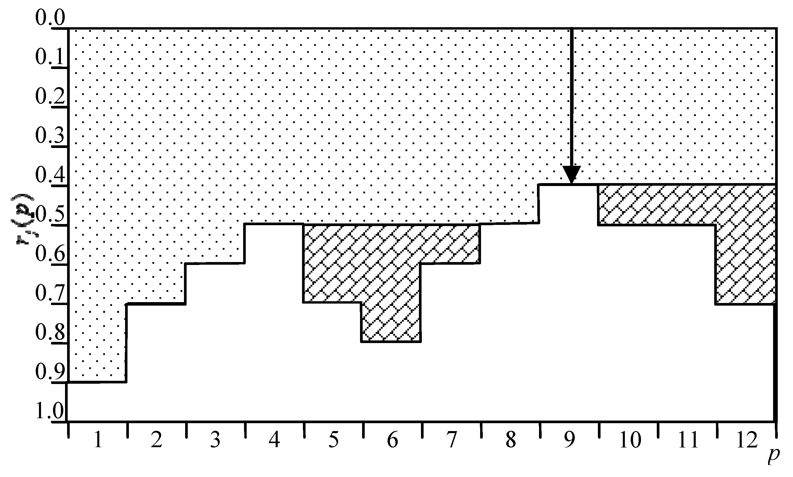
When the latter strategy is adopted, the PoA to be used for the outage rate assessment is related to the minimum value of R_j,m during islanding. It is indicated by an arrow in Figure 4 and it represents the improvement, i.e., the reduction of outage rate that can actually be obtained, thanks to islanding. The PoA to be considered for outage duration assessment is related to the customers not left unsupplied during islanding. It is represented by the dotted area in Figure 4 and it is the reduction, in terms of outage duration, that can actually be obtained through islanding. The bricked area represents the further reduction achievable when the former strategy is adopted, although it involves a worsening in the outage rate that can be even worse than the value obtained when islanding is not adopted. However, both strategies reduce the outage duration.

In [4] it has been proved that telecontrolled sectionalizers strongly reduce (improve) the outage duration but slightly increase (worsen) the outage rate when islanding is permitted. Therefore, considering this, and also the inconvenience of using the first strategy, the second one is considered in the following in order to improve both outage rate and duration by means of islanding.

An analytical model to compute the PoA index to be used for evaluating LP reliability indices when the second strategy is adopted is described in the following. To this purpose, a given time interval T during which the portion of the network downstream from switch j works in island mode of operation is considered. Assuming that there are N time slots in the interval T, a path is defined as the evolution of process $r_j(p)$, and it is given by the sequence of values assumed by $r_j(p)$ in each time slot. The set of all the possible paths that process $r_j(p)$ can assume in the N time slots is called ${\mathsf{\Psi }}_j$, and ${\wp }_j=\langle r_j(1),\mathrm{...},r_j(N)\rangle$ is the generic element of ${\mathsf{\Psi }}_j$. By applying the Chapman–Kolmogorov equation to the Markov model defined so far, the probability of the generic path ${\wp }_j$ in the interval T is computed as follows:

$$w_{{\wp }_j}={\mathsf{\pi }}_{r_j(1)}^{(R_j)}\cdot {\displaystyle \prod _{p=2}^N}{P}_{\left[r_j(p-1),r_j(p)\right]}^{(R_j)}.$$

(13)

By applying the theorem of the total probability, the PoA of an island j, referred to as PoAR_j(T,N), to be considered for outage rate assessment, is computed as:

$$PoA{R}_j\left(T,N\right)={\displaystyle \sum _{{\wp }_j\in {\mathsf{\Psi }}_j}}{w}_{{\wp }_j}{R}_{{\wp }_j},$$

(14)

where $R_{{\wp }_j}$ is the minimum value of the process $r_j(p)$ along the path ${\wp }_j$ (that is, the length of the arrow indicated in Figure 4).

The PoA of an island j, referred to as PoAD_j(T,N), to be considered for outage duration assessment, is computed as follows:

$$PoA{D}_j\left(T,N\right)={\displaystyle \sum _{{\wp }_j\in {\mathsf{\Psi }}_j}}{w}_{{\wp }_j}\frac{1}{N}{\displaystyle \sum _{p=1}^N{\mathsf{\xi }}_j(p)},$$

(15)

where ${\mathsf{\xi }}_j(p)$ is the worst value of $r_j(p)$ up to time slot p along path ${\wp }_j$, that is:

$${\mathsf{\xi }}_j(p)=\underset{\mathsf{\zeta }\in [1,p]}{\min }{\left\{r_j(\mathsf{\zeta })\right\}}^{}.$$

(16)

In other words, PoAD_j(T,N) is obtained by weighting a part of the area delimited by each path (i.e., the dotted area in Figure 4). The weight is the probability that the path occurs.

6. Case Study

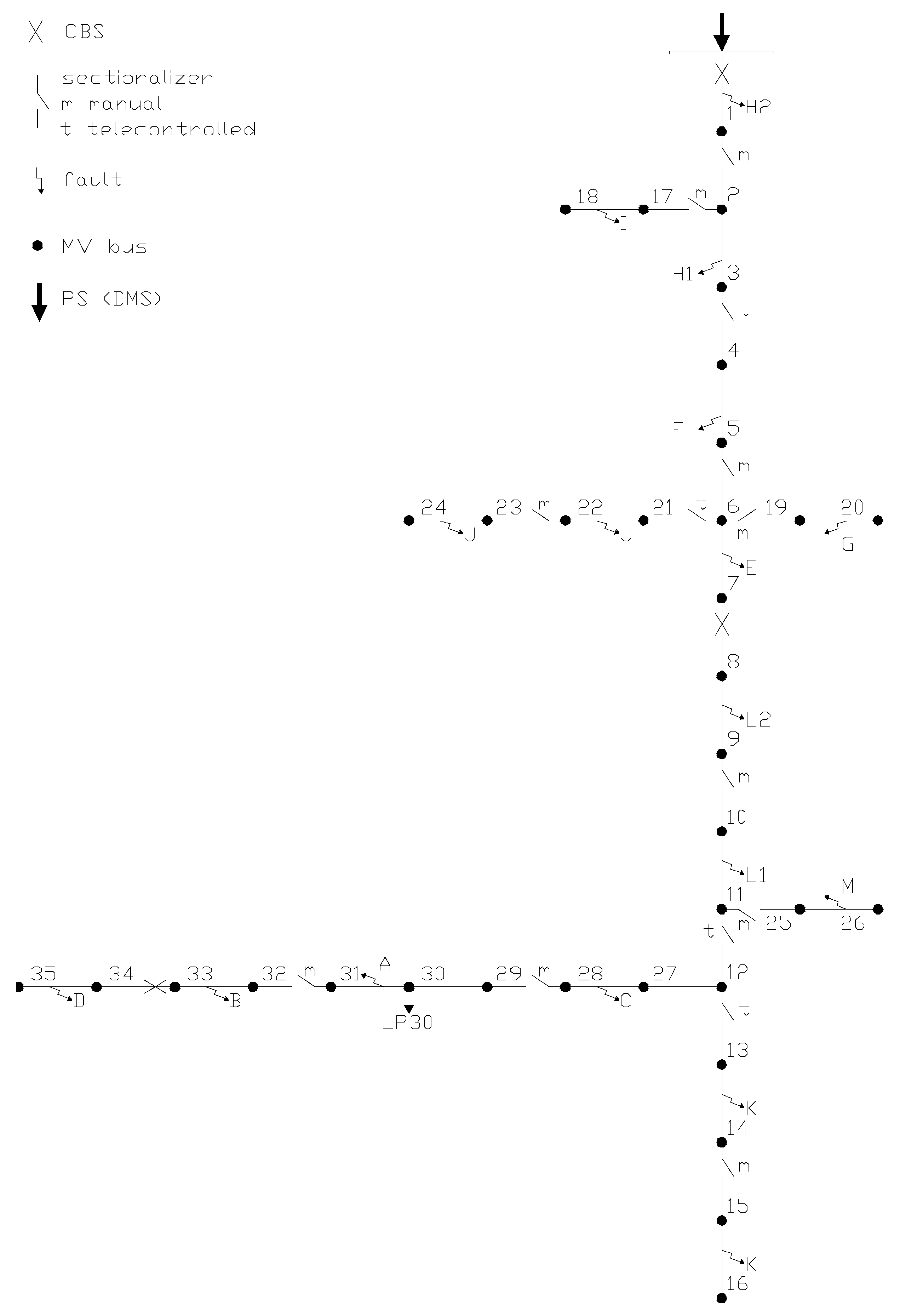
The analytical formulation proposed in this paper is applied to the example distribution network reported in Figure 1 with the aim of providing an accurate measure of the reliability improvement that can be achieved thanks to islanding in distribution networks where telecontrolled CBs, as well as telecontrolled and manual sectionalizers, are installed.

For each branch, the failure rate (i.e., the number of faults per year) and the repair time have been assumed as 0.05 and 8 h, respectively. Both the PS and the switches are considered fully reliable. Each node is considered as a LP with 100 customers. Switching times of 0.1 h and 2 h are assumed for telecontrolled and manual sectionalizers, respectively. The local DGs of each island need 0.08 h to become available (DGs' time to be available).

A set of branches (SOB) that affect a given LP in the same way can be considered as an equivalent branch. In detail, the branches located between switch j and the switches placed downstream from j belong to SOB j. An equivalent branch failure rate and repair time for SOB j are obtained by summing, respectively, the branch failure rates and the normalized repair times of its branches. The normalized repair time of a branch belonging to SOB j is computed by multiplying the failure rate by the repair time of the branch and, subsequently, by dividing the result by the equivalent branch failure rate of j. Similarly, set of nodes (SON) j is defined as the set of nodes located between switch j and the switches placed downstream from it. An SOB affects all the LPs belonging to an SON in the same way, so all the LPs within the same reliability zone have the same annual outage rate and duration [31]. Appendix B reports information about the branches and the nodes belonging to each SOB and SON, respectively; the scenario related to each 2-tuple SON/SOB; the average and max power demand for each LP; the position, average, and max power level for each renewable distributed generator; and the position and rated power of each conventional generator.

As a term of comparison, first the PoA is calculated by means of ${\underset{\_}{\mathsf{\pi }}}^{(R_j)}$, neglecting load and generation fluctuations, thus obtaining ${\mathsf{\rho }}_{A,j}$. On the other hand, the proposed indices for assessing PoA more accurately, $PoA{R}_j\left(T,N\right)$ and $PoA{D}_j\left(T,N\right)$, are obtained by means of $P^{(R_j)}$.

Table 4. PoA computed considering ($PoA{R}_j$;$PoA{D}_j$) and not considering (${\mathsf{\rho }}_{A,j}$); load and generation fluctuations when correlation between load and generation is neglected and not neglected.

Island j	Correlation Neglected			Correlation Not Neglected
	${\mathsf{\rho }}_{A,j}$	$PoA{R}_j\left(8,8\right)$	$PoA{D}_j\left(8,8\right)$	${\mathsf{\rho }}_{A,j}$	$PoA{R}_j\left(8,8\right)$	$PoA{D}_j\left(8,8\right)$
1	0.7781	0.6611	0.7112	0.7783	0.6607	0.7111
2	0.7928	0.6760	0.7264	0.7907	0.6732	0.7239
4	0.7375	0.6185	0.6683	0.7379	0.6196	0.6693
6	0.7825	0.6653	0.7151	0.7826	0.6654	0.7152
8	0.7533	0.6323	0.6833	0.7517	0.6318	0.6823
10	0.8195	0.7055	0.7545	0.8197	0.7073	0.7557
12	0.7275	0.6075	0.6573	0.7271	0.6118	0.6599
13	0.8071	0.7213	0.7588	0.8071	0.7213	0.7588
15	0.9916	0.9892	0.9904	0.9916	0.9892	0.9904
17	0.0000	0.0000	0.0000	0.0000	0.0000	0.0000
19	0.0000	0.0000	0.0000	0.0000	0.0000	0.0000
21	0.4366	0.3754	0.4009	0.4366	0.3754	0.4009
23	0.8201	0.7406	0.7748	0.8201	0.7406	0.7748
25	0.9461	0.9135	0.9296	0.9453	0.9082	0.9265
29	0.8540	0.7273	0.7835	0.8558	0.7348	0.7886
32	0.8485	0.6829	0.7564	0.8563	0.7010	0.7703
34	0.9440	0.9095	0.9265	0.9457	0.9117	0.9285

shows the PoA values for each island of the distribution network reported in Figure 1. If T = 8 h and N = 8 steps, then the duration of each step is one hour. In this case study, the results show that neglecting the correlation between load and generation does not involve inaccurate values. Moreover, the effect of these values on the system indices is negligible because they are slightly overestimated in some cases and slightly underestimated in others.

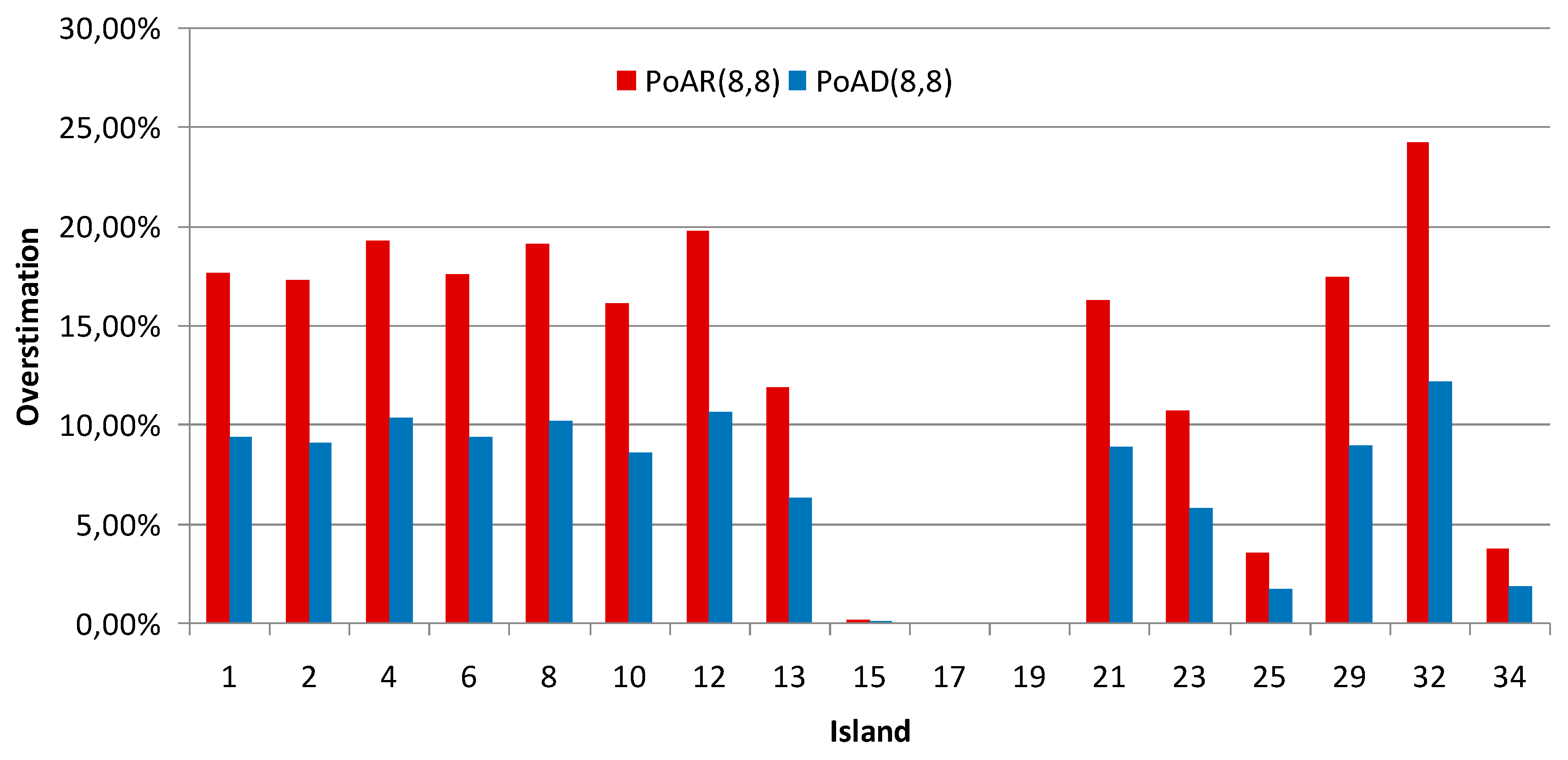
On the other hand, neglecting load and generation fluctuations leads to an overestimation of the ability of DGs to meet the island load, as highlighted by Figure 5. The error in the PoA affecting the LP outage rate is mainly in the interval 15%–20%, and is greater than the error on the PoA affecting outage duration (8%–10%). In a few cases, the error is negligible, such as for islands 15, 25, and 34, because the load is almost always met by local generation. In other words, the Markov process $r_j(p)$ often assumes a value of 1 and consequently generation and load fluctuations do not significantly affect the PoA value.

Table 5. Distribution system reliability indices values when both manual and telecontrolled sectionalizers are installed in the network.

Index	I	II	III	Overestimated Improvement	Actual Improvement	Overestimation on the Improvement
SAIFI	1.270	0.947	1.014	25.43%	20.16%	26.17%
SAIDI	5.329	2.312	2.568	56.61%	51.81%	9.27%

reports the values of the distribution system reliability indices usually adopted for the reward/penalty mechanisms, that is, the System Average Interruption Frequency Index (SAIFI):

$$SAIFI=\frac{{\displaystyle \sum _{i=1}^{n_{LP}}{N}_{C,i}\cdot {\mathsf{\lambda }}_i}}{{\displaystyle \sum _{i=1}^{n_{LP}}{N}_{C,i}}}$$

(17)

and the System Average Interruption Duration Index (SAIDI):

$$SAIDI=\frac{{\displaystyle \sum _{i=1}^{n_{LP}}{N}_{C,i}\cdot U_i}}{{\displaystyle \sum _{i=1}^{n_{LP}}{N}_{C,i}}},$$

(18)

where $n_{LP}$ is the number of LPs in the network, $N_{C,i}$ is the number of customers connected to LP i, and ${\mathsf{\lambda }}_i$ and $U_i$ are the outage rate and duration of LP i that can be computed by using the formulation reported in Appendix A, respectively. SAIFI and SAIDI have been computed for the network in Figure 1, where manual and telecontrolled sectionalizers are installed. Three different cases have been considered:

(i).

islanding is not permitted by regulation;

(ii).

islanding is permitted by regulation, but load and generation fluctuations are neglected;

(iii).

islanding is permitted by regulation and both load and generation fluctuations are considered by using of the proposed analytical model.

The results presented in Table 5 show that both network reliability indices are overestimated when the aforementioned fluctuations occurring during islanding are neglected. For example, the actual improvement in SAIFI is about 20% when islanding is permitted by regulations (1.014 vs. 1.270), but the improvement is overestimated when load and generation fluctuations are neglected. More specifically, an improvement of about 25% appears when considering the index value evaluated by neglecting fluctuations (0.947 vs. 1.270). Therefore, the overestimated improvement is 26.17% greater than the actual one. As is expected from the results in Table 4, the overestimation of SAIFI improvement is greater than for SAIDI. Similar considerations hold when only manual sectionalizers are installed, as highlighted by the results in

Table 6. Distribution system reliability indices values when only manual sectionalizers are installed in the network.

Index	I	II	III	Overestimated Improvement	Actual Improvement	Overestimation on the Improvement
SAIFI	1.270	0.929	0.992	26.85%	21.89%	22.66%
SAIDI	6.020	3.146	3.389	40.96%	36.40%	12.53%

.

The results have confirmed that in a network with both manual and telecontrolled sectionalizers, islanding improves SAIFI less (20.16% vs. 21.89%) than when only manual sectionalizers are installed. On the other hand, when both kinds of sectionalizers are installed, the SAIDI improvement is greater than that achievable with only manual sectionalizers (51.81% vs. 36.40%). In other words, the results confirm that telecontrolled sectionalizers strongly improve the outage duration against a slightly worsening in the outage rate when islanding is permitted. Moreover, both reliability indices improve when telecontrolled sectionalizers are installed and the proposed strategy (discussed in Section 5) is adopted to manage load and generation fluctuations during islanding. Finally, when islanding is not permitted by regulation, SAIDI is reduced by more than 10% when telecontrolled sectionalizers are added to the network (5.329 vs. 6.020).

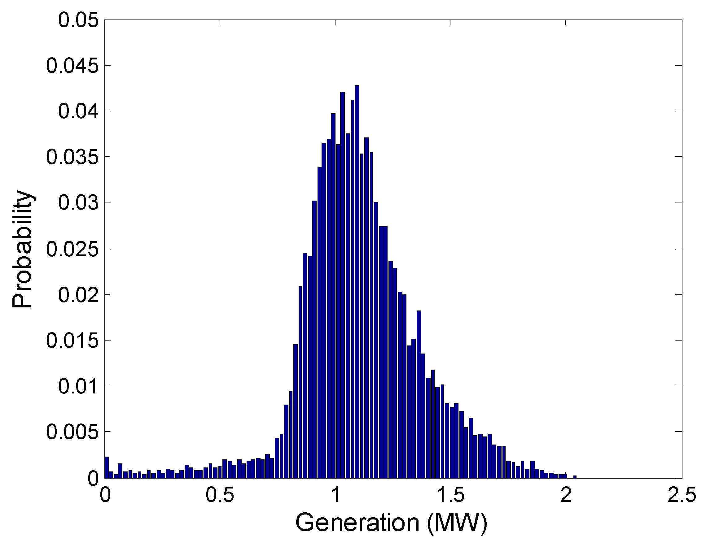
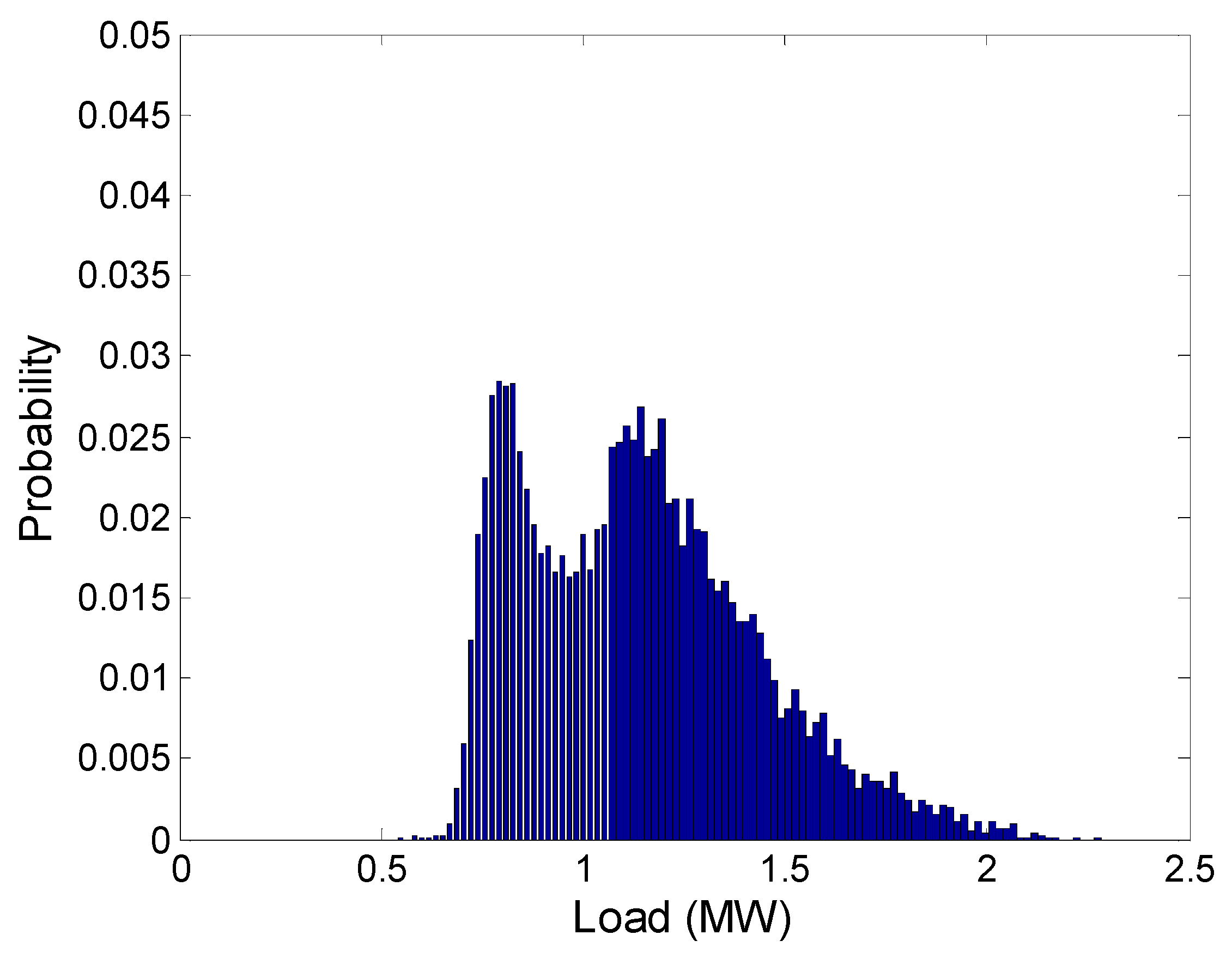
By way of example, in the following it is considered that island 32 exhibits the greatest overestimation of PoA. The probability density functions of the equivalent load and generator present in it are shown in Figure 6 and Figure 7, respectively.

In

Table 7. Transition probability matrix of the equivalent load (kW) of island 32, $P^{(D_{32})}$.

$P^{(D_{32})}$	628	802	976	1150	1325	1499	1673	1847	2021	2196
628	0.28	0.71	0.01	0	0	0	0	0	0	0
802	0.03	0.77	0.17	0.03	0	0	0	0	0	0
976	0	0.25	0.45	0.28	0.02	0	0	0	0	0
1150	0	0.01	0.22	0.55	0.20	0.02	0	0	0	0
1325	0	0	0.04	0.29	0.47	0.19	0.02	0	0	0
1499	0	0	0	0.04	0.34	0.41	0.19	0.02	0	0
1673	0	0	0	0	0.09	0.34	0.38	0.17	0.02	0
1847	0	0	0	0	0	0.15	0.31	0.41	0.13	0
2021	0	0	0	0	0	0	0.06	0.47	0.39	0.08
2196	0	0	0	0	0	0	0	0.22	0.33	0.44

,

Table 8. Transition probability matrix of equivalent generation (kW) of island 32, $P^{(G_{32})}$.

$P^{(G_{32})}$	102	307	512	717	922	1127	1332	1537	1741	1946
102	0.43	0.23	0.09	0.15	0.08	0.03	0	0	0	0
307	0.19	0.22	0.25	0.13	0.13	0.07	0.01	0	0	0
512	0.05	0.09	0.25	0.20	0.28	0.09	0.05	0	0	0
717	0.03	0.02	0.09	0.27	0.39	0.18	0.02	0	0	0
922	0	0.01	0.01	0.05	0.49	0.38	0.05	0	0	0
1127	0	0	0	0.02	0.32	0.45	0.17	0.03	0	0
1332	0	0	0	0.01	0.08	0.35	0.35	0.15	0.05	0.01
1537	0	0	0	0	0.02	0.15	0.37	0.31	0.13	0.02
1741	0	0	0	0.01	0.02	0.03	0.25	0.38	0.24	0.06
1946	0	0	0.02	0	0	0	0.10	0.45	0.25	0.18

,

Table 9. Transition probability matrix of R in island 32, $P^{(G_{32})}$.

$P^{(R_{32})}$	0.0943	0.1897	0.2850	0.3803	0.4757	0.5710	0.6663	0.7617	0.8570	0.9523
0.0943	0.42	0.08	0.10	0.08	0.05	0.05	0.07	0.05	0.04	0.05
0.1897	0.20	0.18	0.09	0.16	0.10	0.10	0.07	0.04	0.03	0.03
0.2850	0.16	0.04	0.17	0.08	0.14	0.12	0.09	0.08	0.02	0.10
0.3803	0.08	0.04	0.05	0.18	0.14	0.16	0.15	0.06	0.06	0.09
0.4757	0.02	0.01	0.03	0.06	0.26	0.33	0.13	0.10	0.03	0.04
0.5710	0.01	0.01	0.01	0.02	0.10	0.34	0.21	0.17	0.10	0.05
0.6663	0.01	0	0	0.01	0.03	0.16	0.24	0.22	0.15	0.17
0.7617	0	0	0	0	0.01	0.09	0.15	0.27	0.13	0.34
0.8570	0	0	0	0	0.01	0.07	0.14	0.18	0.24	0.36
0.9523	0	0	0	0	0	0	0.02	0.07	0.05	0.85

and

Table 10. Steady-state probability array of the process $r_{32}(p)$, ${\underset{\_}{\mathsf{\pi }}}^{(R_{32})}$.

Value	Probability
0.0943	0.0085
0.1897	0.0029
0.2850	0.0046
0.3803	0.0072
0.4757	0.0183
0.5710	0.0616
0.6663	0.0801
0.7617	0.1249
0.8570	0.0867
0.9523	0.6053

are reported detailed results for the considered island. More specifically, Table 7 shows the transition probability matrix related to the equivalent load of the island 32, $P^{(D_{32})}$. Both the first row and the first column report the power absorbed in that island. From the structure of this matrix it can be deduced that the process is strongly autocorrelated. In other words, there is a high probability that the state variable remains constant or changes to an adjacent state in the transition from one time slot to the following one. Similarly, the transition probability matrix related to the equivalent generation of island 32, $P^{(G_{32})}$ is shown in Table 8. From this table it can be noticed that the process modeling the island generation is less correlated than the process modeling the load.

The quantized transition probability matrix, $P^{(R_{32})}$, shown in Table 9, is derived by elaborating the previous matrices. In particular, through the Kronecker product between the matrices $P^{(D_{32})}$ and $P^{(G_{32})}$, a $100\times 100$ matrix $P^{(R_{32})}$ is obtained. This matrix has been quantized to 10 levels and the relative transition probabilities have been aggregated. The system steady-state probability values of ${\underset{\_}{\mathsf{\pi }}}^{(R_{32})}$, reported in Table 10, are estimated from matrix $P^{(R_{32})}$ according to Equation (12).

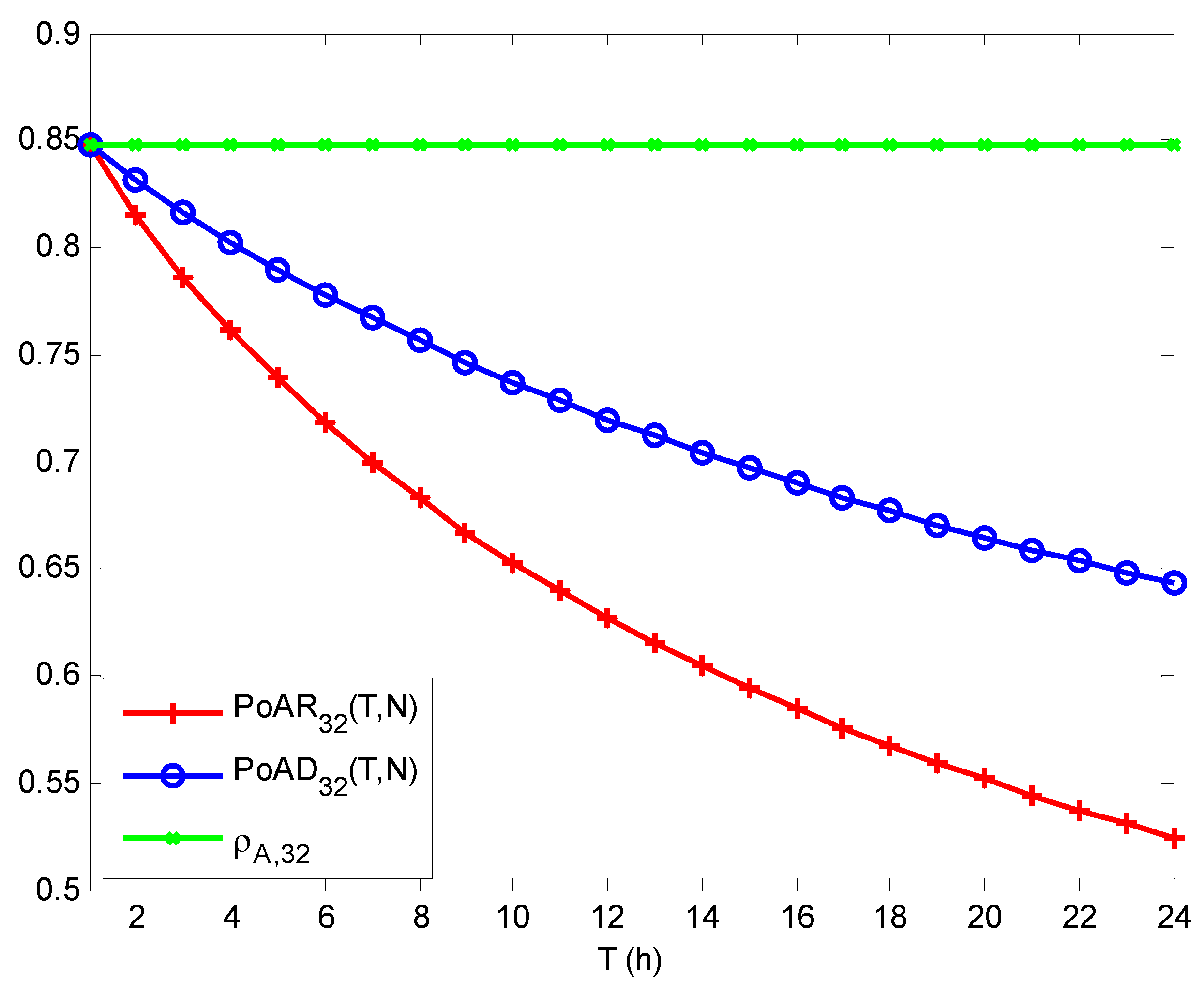
Finally, Figure 8 shows the variation of $PoA{R}_{32}\left(T,N\right)$ and $PoA{D}_{32}\left(T,N\right)$ with T when a duration of one hour is considered. The results highlight that the greater the time interval in which the island mode is maintained, the greater the overestimation of the PoA and, consequently, the benefits of islanding being overvalued. Moreover, the results confirm that the error in the PoA to be considered for outage rate computation is greater than the one for computing outage duration, and also show that the difference increases with the duration of the islanding period.

7. Conclusions

This paper has presented an analytical formulation to assess distribution system reliability in networks where intentional islanding is permitted by regulation, and all circuit breakers and some sectionalizers are telecontrolled. The considered protection scheme exploits a delayed operation of the circuit breakers to perform logic selectivity. During the delay, a centralized control system receives information about the fault current direction from the circuit breakers detecting the fault, and sends an opening authorization to the circuit breakers that have to be opened. Typically, the delay is around 100 ms, and the smart communications subsystems enabling this protection scheme play a fundamental role in the behavior of the whole network. The main wireless and wired telecommunications technologies have been considered and compared, highlighting their installation and maintenance costs, and their appropriateness to the specific case of allowing the DMS to manage faults in order to guarantee safety and respect the maximum delay requirements.

The formulation proposed for computing the adequacy of island generation is based on a Markov chain that models the ratio between load and generation in order to represent the fluctuation during islanding of load and green-energy generators. The results have shown that network reliability indices are overestimated when the aforementioned fluctuations occurring during intentional islanding are neglected. Moreover, the overestimation of SAIFI improvement is greater than for SAIDI.

References

1. Mcgranaghan, M.F. Quantifying reliability and service quality for distribution systems. IEEE Trans. Ind. Appl. 2007, 43, 188–195. [Google Scholar] [CrossRef]
2. Shourkaei, H.M.; Jahromi, A.A.; Firuzabad, M.F. Incorporating service quality regulation in distribution system maintenance strategy. IEEE Trans. Power Deliv. 2011, 26, 2495–2504. [Google Scholar] [CrossRef]
3. Goroohi Sardou, I.; Banejad, M.; Hooshmand, R.; Dastfan, A. Modified shuffled frog leaping algorithm for optimal switch placement in distribution automation system using a multi-objective fuzzy approach. IETGener. Transm. Distrib. 2012, 6, 493–502. [Google Scholar] [CrossRef]
4. Conti, S.; Rizzo, S.A.; El-Saadany, E.F.; Essam, M.; Atwa, Y.M. Reliability assessment of distribution systems considering telecontrolled switches and microgrids. IEEE Trans. Power Syst. 2014, 29, 598–607. [Google Scholar] [CrossRef]
5. Conti, S.; Nicolosi, R.; Rizzo, S.A. Generalized systematic approach to assess distribution system reliability with renewable distributed generators and microgrids. IEEE Trans. Power Deliv. 2012, 27, 261–270. [Google Scholar] [CrossRef]
6. Bauen, A. Future energy sources and systems—Acting on climate change and energy security. J. Power Sources 2006, 157, 893–901. [Google Scholar] [CrossRef]
7. European Commission—Climate strategies & targets—2020 climate & energy package. Available online: http://ec.europa.eu/clima/policies/strategies/2020/index_en.htm (accessed on 4 May 2016).
8. Fang, X.; Misra, S.; Xue, G.; Yang, D. Smart grid—Thenew and improved power grid: A survey. IEEE Commun. Surv. Tutor. 2012, 14, 944–980. [Google Scholar] [CrossRef]
9. Ipakchi, A.; Albuyeh, F. Grid of the future. IEEE Power Energy Mag. 2009, 7, 52–62. [Google Scholar] [CrossRef]
10. Cerretti, A.; Di Lembo, G.; di Primo, G.; Gallerani, A.; Valtorta, G. Automatic fault clearing on MV networks with neutral point connected to ground through impedance. In Proceedings of the CIRED 17th International Conference on Large Electricity Distribution, Barcelona, Spain, 12–15 May 2003.
11. Gungor, V.C.; Sahin, D.; Kocak, T.; Ergut, S.; Buccella, C.; Cecati, C.; Hancke, G.P. Smart grid technologies: Communication technologies and standards. IEEE Trans. Ind. Inform. 2011, 7, 529–539. [Google Scholar] [CrossRef]
12. Billinton, R.; Allan, R.N. Reliability Evaluation of Power Systems, 2nd ed.; Plenum Press: New York, NY, USA; London, UK, 1996. [Google Scholar]
13. Billinton, R.; Bagen, B. Generating capacity adequacy evaluation of small stand-alone power systems containing solar energy. Reliab. Eng. Syst. Saf. 2006, 91, 438–443. [Google Scholar] [CrossRef]
14. Franco, A.; Salza, P. Strategies for optimal penetration of intermittent renewables in complex energy systems based on techno-operational objectives. Renew. Energy 2011, 32, 743–753. [Google Scholar] [CrossRef]
15. Beritelli, F.; Lombardo, A.; Palazzo, S.; Schembra, G. Performance analysis of an ATM multiplexer loaded with VBR traffic generated by multimode speech coders. IEEE J. Sel. Areas Commun. 1999, 17, 63–81. [Google Scholar] [CrossRef]
16. Kubik, M.L.; Coker, P.J.; Barlow, J.F.; Hunt, C. A study into the accuracy of using meteorological wind data to estimate turbine generation output. Renew. Energy 2013, 51, 153–158. [Google Scholar] [CrossRef]
17. Hart, E.K.; Jacobson, M.Z. A Monte Carlo approach to generator portfolio planning and carbon emissions assessments of systems with large penetrations of variable renewables. Renew. Energy 2011, 36, 2278–2286. [Google Scholar] [CrossRef]
18. Wang, J.; Botterud, A.; Bessa, R.; Keko, H.; Carvalho, L.; Issicaba, D.; Sumaili, J.; Miranda, V. Wind power forecasting uncertainty and unit commitment. Appl. Energy 2011, 88, 4014–4023. [Google Scholar] [CrossRef]
19. Noor, S.F.; McDonald, J.R. Forced-outage rates of generating units based on expert evaluation. IEEE Trans. Reliab. 1996, 45, 138–140. [Google Scholar] [CrossRef]
20. Akyildiz, I.F.; Wang, X. A survey on wireless mesh networks. IEEE Commun. Mag. 2005, 43, S23–S30. [Google Scholar] [CrossRef]
21. Wang, K.; Ramanathan, P. End-to-end delay assurances in multihop wireless local area networks. In Proceedings of the IEEE Global Telecommunications Conference, San Francisco, CA, USA, 1–5 December 2003; Volume 5, pp. 2962–2966.
22. Khalaf, R.; Rubin, I. Throughput and delay analysis in single hop and multihop IEEE 802.11 networks. In Proceedings of the 3rd International Conference on Broadband Communications, Networks and Systems, San Jose, CA, USA, 1–5 October 2006; pp. 1–9.
23. Bisnik, N; Abouzedi, A. Delay and throughput in random access wireless mesh networks. IEEE Int. Conf. Commun. 2006, 1, 403–408. [Google Scholar]
24. Grazia, C.A.; Klapez, M.; Patriciello, N.; Casoni, M. PINK: Proactive INjection into acK, a queue manager to impose fair resource allocation among TCP flows. In Proceedings of the IEEE 11th International Conference on Wireless and Mobile Computing, Networking and Communications (WiMob), Abu Dhabi, United Arab Emirates, 19–21 October 2015; pp. 125–131.
25. Snoeren, A.C. Adaptive inverse multiplexing for wide-area wireless networks. In Proceedings of the GLOBECOM ′99 Global Telecommunications Conference, Rio de Janeiro, Brazil, 5–9 December 1999; Volume 3, pp. 1665–1672.
26. Abdelrahma, T.; Mustafa, A.B.A.; El-Azhary, I. Evolution of the quality of service (QOS) parameters for the short message service (SMS): Review paper. IOSR J. Eng. 2014, 14, 34–38. [Google Scholar] [CrossRef]
27. Negreira, J.A.; Pereira, J.; Belzarena, P.; Pérez, S. End-to-end measurements over GPRS-EDGE networks. In Proceedings of the 4th International IFIP/ACM Latin American Conference on Networking, San José, Costa Rica, 10–11 October 2007; pp. 121–131.
28. Galli, S.; Scaglione, A.; Wang, Z. For the grid and through the grid: The role of power line communications in the smart grid. Proc. IEEE 2011, 99, 998–1027. [Google Scholar]
29. Buchholz, P.; Kemper, P. Kroneckerbased matrix representations for large Markov models, validation of stochastic systems: A guide to current research. Lect. Notes Comput. Sci. 2004, 2925, 256–295. [Google Scholar]
30. Arya, L.D.; Choube, S.C.; Arya, R.; Tiwary, A. Evaluation of reliability indices accounting omission of random repair time for distribution systems using Monte Carlo simulation. Int. J. Electr. Power Energy Syst. 2012, 42, 533–541. [Google Scholar] [CrossRef]
31. Pregelj, A.; Begovic, M.; Rohatgi, A. Recloser allocation for improved reliability of DG-enhanced distribution networks. IEEE Trans. Power Syst. 2007, 21, 1442–1449. [Google Scholar] [CrossRef]
32. Conti, S.; Rizzo, S.A. Probability of adequacy evaluation considering power output correlation of renewable generators in smart grids. Int. J. Electr. Power Energy Syst. 2014, 61, 145–151. [Google Scholar] [CrossRef]
Figure 1. Example of distribution network presenting all the possible “scenarios” that can occur in a radial network. The capital letter next to each fault shows the related scenario reported in Appendix A.
Applsci 06 00138 g001
Figure 2. Time evolution of the fault clearing process.
Applsci 06 00138 g002
Figure 3. Quantization of the power demand.
Applsci 06 00138 g003
Figure 4. Improvement in term of outage rate (arrow) and duration (dotted area) achievable thanks to islanding for a path when the island management strategy aims at maximizing the reduction of the outage rate. The bricked area represents the further reduction achievable when the strategy aiming at maximizing the reduction of the outage duration is adopted, although it involves a worsening in the outage rate.
Applsci 06 00138 g004
Figure 5. Overestimation of the Probability of Adequacy computed not considering ( ρ A , j ) load and generation fluctuations during islanding with respect to the value obtained accounting for them.
Applsci 06 00138 g005
Figure 6. Probability density function of the equivalent load in island 32.
Applsci 06 00138 g006
Figure 7. Probability density function of the equivalent generation in island 32.
Applsci 06 00138 g007
Figure 8. PoA variation with duration of islanding operation in island 32.
Applsci 06 00138 g008