
Dynamical Systems for Audio Synthesis: Embracing Nonlinearities and Delay-Free Loops †

Department of Music, University of California, San Diego, CA 92093, USA
†
This paper is an extended version of our paper published in the 41st International Computer Music Conference (ICMC), Denton, TX, USA, 25 September–1 October 2015.
Appl. Sci. 2016, 6(5), 134; https://doi.org/10.3390/app6050134
Submission received: 1 February 2016
/
Revised: 19 April 2016
/
Accepted: 27 April 2016
/
Published: 10 May 2016
(This article belongs to the Special Issue Audio Signal Processing)
Abstract
:Many systems featuring nonlinearities and delay-free loops are of interest in digital audio, particularly in virtual analog and physical modeling applications. Many of these systems can be posed as systems of implicitly related ordinary differential equations. Provided each equation in the network is itself an explicit one, straightforward numerical solvers may be employed to compute the output of such systems without resorting to linearization or matrix inversions for every parameter change. This is a cheap and effective means for synthesizing delay-free, nonlinear systems without resorting to large lookup tables, iterative methods, or the insertion of fictitious delay and is therefor suitable for real-time applications. Several examples are shown to illustrate the efficacy of this approach.
Keywords:
digital signal processing; sound synthesis and modeling; dynamical systems; virtual analog; physical modelingPACS:
J01011. Introduction
There are certain continuous-time systems that are of interest to computer musicians, that contain a delay-free loop—instantaneous feedback from the output to the input. These are said to be ‘non-computable loops’ because in order to process the input, one needs to know the output, which hasn’t been computed yet.
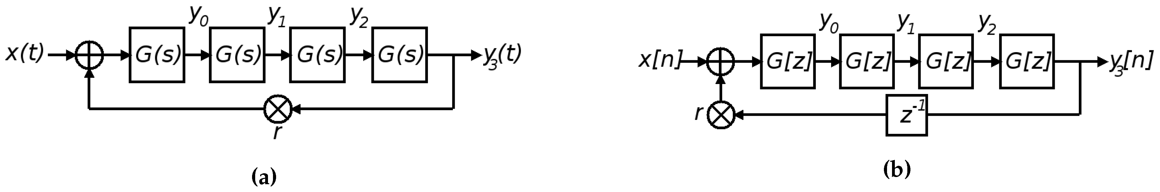
The most straightforward way to deal with this problem is to insert a small amount of delay in the feedback loop. This was done, for example, in one of the earliest considerations of digitizing the Moog ladder filter [1]. In that case, the analog circuitry under consideration contains a delay-free path from output to input in its continuous-time block diagram. The authors add unit delay () to the structure in order to make it computable (Figure 1). This has the unwanted side-effect, however, of coupling the resonance parameter of the filter to the parameter governing cutoff frequency.
The circuit emulation software SPICE (Simulation Program with INtegrated Circuit Emphasis) [2] can compute systems with delay-free loops through the use of iterative solvers. SPICE is very robust and is still the gold standard against which to demonstrate accuracy in virtual analog literature. It is not, however, well suited for virtual instrument design since it is not meant to be run in real-time. It is also unsuitable for describing systems that are not represent-able as electrical circuits.
A class of structures that can also emulate circuits (and other things) in real-time are wave digital filters (WDFs). WDFs were first introduced in the early 1970’s [3] and have been the subject of a steady stream of study since then. More recently, there has been increased development of WDF theory in the digital audio community, particularly in circuit simulation applications [4,5,6], but in virtual acoustics as well [7,8,9]. Until very recently, however, WDF theory was not sufficient for representing systems involving delay-free loops. To this end, the K-method [10] has been suggested as a means of solving coupled, multivariate nonlinearities in WDFs [11,12].
Interestingly, the K-method was originally proposed in [10] as a means of eliminating delay-free loops in virtual acoustic models. Nevertheless, it and its variants are frequently used in circuit simulation applications [13,14,15]. The K-method operates on dynamical state-space systems that are of the form:
where is the ‘state’, is an input vector, is the output and is a nonlinear vector function of .
After discretizing the system, the nonlinearity in Equation (3) can be solved with an iterative solver such as Newton-Raphson method. Furthermore multidimensional lookup tables can be pre-computed to avoid convergence issues, rendering the solution more suitable to real-time computation. The method also requires discretizing Equation (1) (e.g., with Backward Euler or the trapezoidal rule). A consequence of this is that if an adjustable parameter presents itself in the discretized version of matrix it may be the case that multiple matrix inversions need to be performed in order to find the correct discretized coefficients that correspond to , , etc. There are times when analysis can resolve this issue (as in [15]), but this can potentially lead to significant slowdown if controllable parameters are desired.
If is linear or if it is a low order polynomial, an exact solution be found to the system and resorting to such methods may not be necessary. However, this is not always the case. We present several examples from a class of nonlinear dynamical systems with delay-free loops that can be solved explicitly without resorting to iteration, tabulation or frequent re-calculation of filter coefficients. Namely, we examine systems in which each node of the network is expressed as an ordinary differential equation (ODE). Consider, for example:
where x and y are states, are functions (perhaps nonlinear) and u is some (perhaps 0 valued) input.
Equations (4) and (5) differ from Equations (1)–(3) in that in Equations (4) and (5), each equation is an explicit ODE whereas only Equation (1) in the other system is a differential one. Most importantly, is not an ODE and Equation (3) is implicit (v is a function of itself). On the other hand, since Equations (4) and (5) are both explicit ODEs, they can be directly solved using explicit numerical methods. Since numerical solvers to ODEs can compute both x and y, the fact that both variables are fed back to the nonlinear functions and in a delay-free loop does not doom us to non-computability.
2. Methods
The solver used in each example below is explicit fourth order Runge-Kutta (RK4):
The subscript i in Equations (6)–(10) is to indicate that there can be N functions () with inputs —which is some computable value. Each node (each ODE that we solve for) has only one output value (the updated state at time , but the value , which we take to be an ‘input’ to the ODE, can be any parameterized combination, linear or not, of all the states in the network; and, if desired, external input.
The time-step h used here is simply the inverse of the sampling frequency: for most of the examples shown below. RK4 is chosen because it is explicit, commonly used, and fourth order accurate. It is beyond the scope of this paper to describe the accuracy and numerical stability of RK4 and compare it to other, similar solvers. The curious reader may be referred to chapter 3 in [16] for a thorough investigation of this topic as it pertains to audio synthesis. It is worth noting, however, that RK4 does not always guarantee stability.
Using a C language application programming interface (API) written by the author, a system of interconnected ODEs can be declared and (through the use of helper functions) passed to an implementation of RK4 that will solve each network node at every time-step. The API also allows for control objects (for adjusting function parameters) to be declared. These can then be manipulated in real-time while the audio engine is running. This API was used to create a Pure Data [17] (Pd) extern to produce the data shown in the examples below. As a creation argument, the extern takes the path to a shared object (a compiled C file with loadable functions) which specifies the functions to be solved, the network topology, and any required control inputs to adjust function parameters. The extern automatically creates the correct number of inlets and outlets and control values can be passed via Pd’s messaging system. Having such an infrastructure for designing, controlling and solving systems such as that given in Equations (4) and (5) is a potentially powerful tool for computer musicians.
This technique of declaring a system of inter-connected ODEs to a software application which will then compute the solution to each node on the network is referred to as ‘unsampled digital synthesis’ (UDS) in a recent paper given at the 2015 International Computer Music Conference [18]. The application of numerical solvers to ODEs is not new in digital audio. The technique has been used, for example, to model diodes in guitar distortion circuitry [19,20]. Furthermore, such a scheme is essentially a subset of the more general family of techniques known as finite difference methods, whose use in digital audio applications is well studied [21].
3. Results
Below are a number of examples of sound synthesis routines that are networks of coupled ODEs solved using RK4.
3.1. Basic Example: Simple Harmonic Motion
Simple harmonic motion can be modeled as a spring-mass mechanism. In this model, the acceleration of the mass is proportional to its position. The proportion depends on the value of the mass and the stiffness of the spring:
here, m is the mass, and k is the spring constant. Since we will consistently be relating rates of change over time, we will drop the time variable t when speaking of these dynamical models. We will use the conventional ‘dot’ notation to denote the time derivative.
Equation (11) is a second order differential equation, but we may render it a first order system in the usual way:
In this formulation the introduced variable is the velocity of the system. By scaling this variable by the resonant angular frequency, we arrive at a more symmetrical form in which both x and the variable y are now in the same units (position):
The frequency of this system is Hz. We note that Equations (13) and (14) is an equivalent system to the the one given in Equation (11) when . Differentiating Equation (13) yields and substituting Equation (14) for yields . The outputs of this system (which we are interested in hearing) are the changing values x and y, which we get by integrating (in this case with RK4) and .
The amplitude and initial phase of the system are given by initial conditions. The amplitude is simply and the phase is .
This implementation of simple harmonic motion is not new in digital audio. Mathews and Smith used oscillators in a similar form to design high-Q bandpass filters [22]; and, this oscillator is analyzed quite thoroughly in Chapter 3 of [21]. In that work it is presented as a basic building block for lumped networks.
By way of contrast, a more frequent implementation of a harmonic oscillator is the lookup oscillator (also called a wavetable oscillator). This consists of a phase signal that references values in a pre-computed table containing one period of a sinusoidal waveform. Oscillators of this variety are covered in most any introductory text to digital audio, for example Chapter 2 in [23]. The lookup oscillator can be generalized to lookup any arbitrary waveform, but we restrict ourselves to the sinusoidal case:
where is a phase signal and (as usual) .
3.2. Reciprocal Sync
Oscillator ‘sync’ is a classic technique from modular analog systems in which a ‘slave’ oscillator has its phase reset to 0 if another ‘master’ oscillator’s output crosses a certain threshold θ. This is a convenient way to create spectrally rich, periodic output.
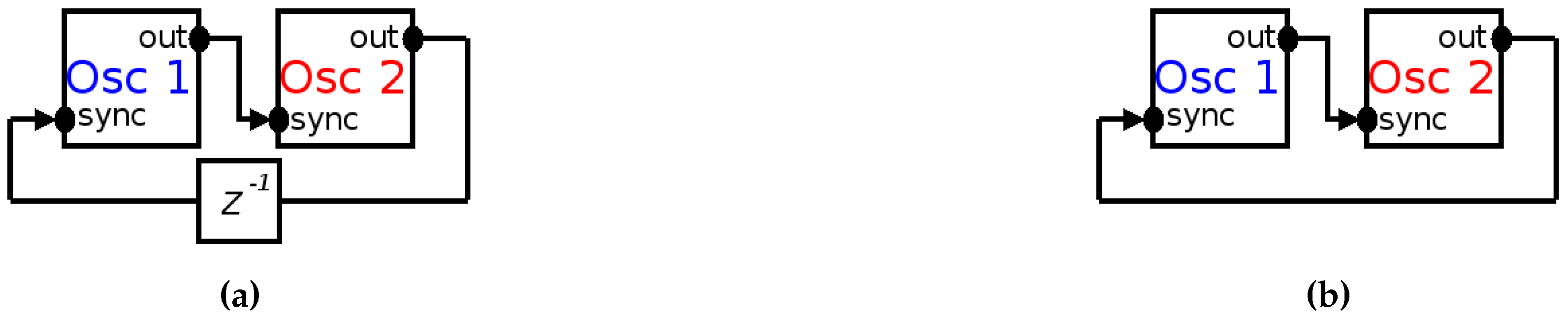
If this routine is computed with lookup oscillators, the order of operations is important. Depending on whether or not the output of the master or slave oscillator is computed first, the output waveforms will be different. This scheduling issue, which results from delay in the feedback loop (depicted in Figure 2a), suggests that lookup oscillators are not ideal for representing two oscillators that sync each other in a tight feedback loop. However, if we model each oscillator as a dynamical system as in Equations (13) and (14), the discrete output of the whole system is computed at once. That is to say, there is no delay between the output of one oscillator and the input of another, as in Figure 2b.
Using a sync rule, we may couple two digital ODE + RK4 oscillators. The rule is that if the state of for one of the oscillators crosses a threshold, the phase of the other will re-initialize. In the case of oscillator 1:
where there is another master/slave oscillator with a subscript of 2.
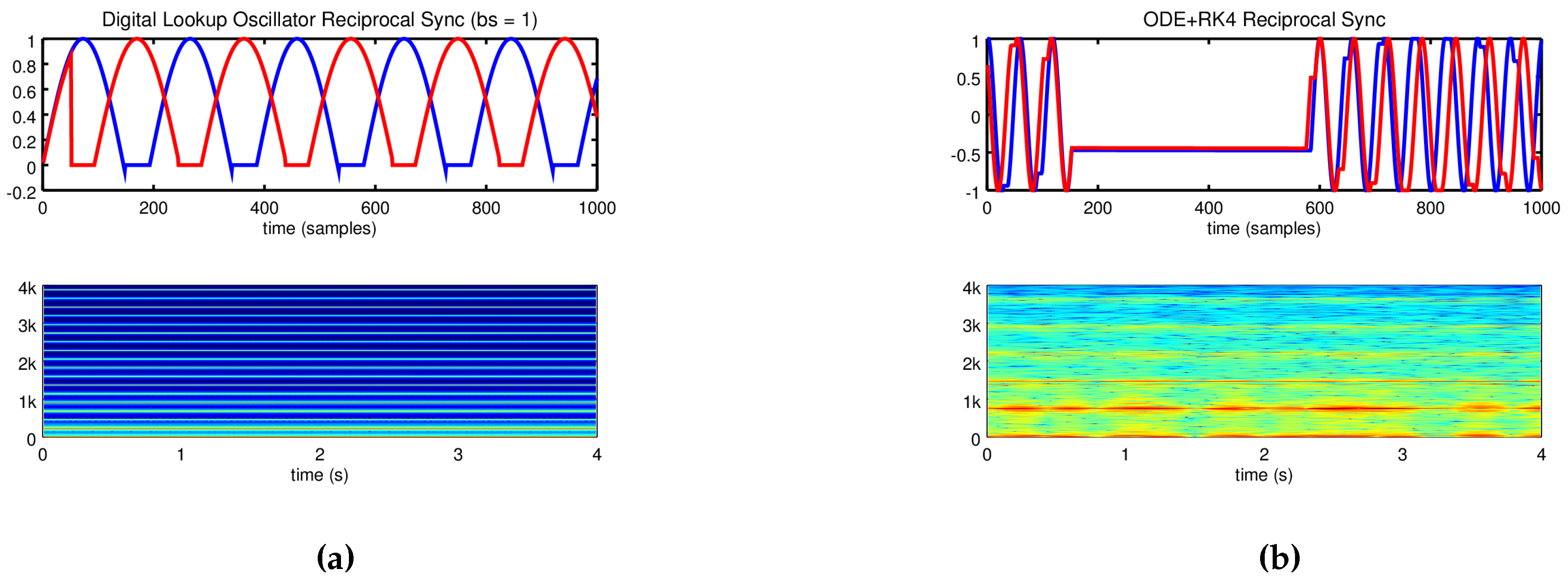
This is simply a nonlinear modification to the Equations (13) and (14). Here, is a gain factor that speeds the return to the ‘zero’ phase (, ). This rule is necessary, because if we are computing our state updates by adding approximate integrations of time derivatives (which is exactly what we do with RK4), then there is no simple way to describe instantaneous jumps from one state to another one that is far away. In the regime of reciprocal sync, each oscillator is both master and slave to the other. As can be seen in Figure 3, our dynamical models shows chaotic behavior which does not appear at all in the lookup oscillator implementation.
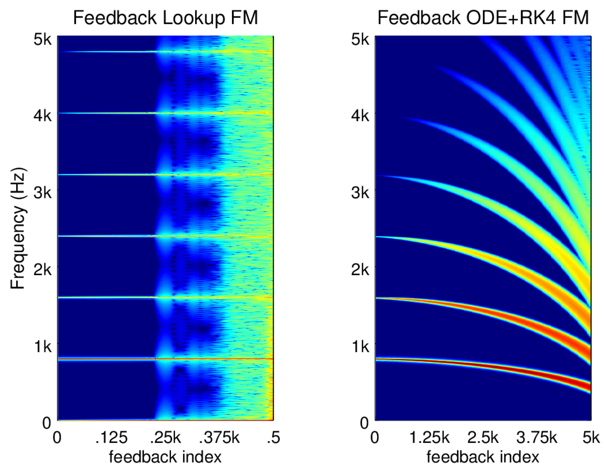
3.3. Reciprocal Frequency Modulation
Frequency Modulation (FM) is a tried and true computer audio technique that has been used to simulate the human voice and many other real musical instruments [24]. In FM the scaled output of one oscillator (the modulator) affects the frequency of another (the carrier). In continuous-time, it can be expressed:
where A is the so-called modulation index, is the angular frequency of the carrier, and is the angular frequency of the modulator. A lookup oscillator digitization of Equation (18) would be:
where is simply the output of some other oscillator of the form shown in Equation (15). The frequencies in the spectrum of the carrier oscillator are predictable depending on and . If and are harmonically related, so are the resulting sidebands (the effects of foldover excepted). The amplitudes of these sidebands depend on A. For a thorough discussion, consult Chapter 5.5 in [23] or any other introductory text on digital audio effects. The implementation in Equation (19) is more precisely called ‘phase modulation’, because the phase signal is modulated [25].
We can implement a reciprocal FM network by again modifying the Equations (13) and (14) and solving with RK4.
here, there are any number of oscillators that modulate one another, and is some linear combination of (the x part of) each other’s outputs:
The coefficients define the index of modulation acting on the frequency of oscillator i by oscillator j.
If we wish to modulate the modulating oscillator with the output of the carrier as in Figure 4, lookup oscillators will be insufficient for the same reasons as described above in the case of reciprocal sync. However we can incorporate a delay-free loop between oscillators by using RK4 to solve for any number of oscillators expressed by Equations (20)–(22).
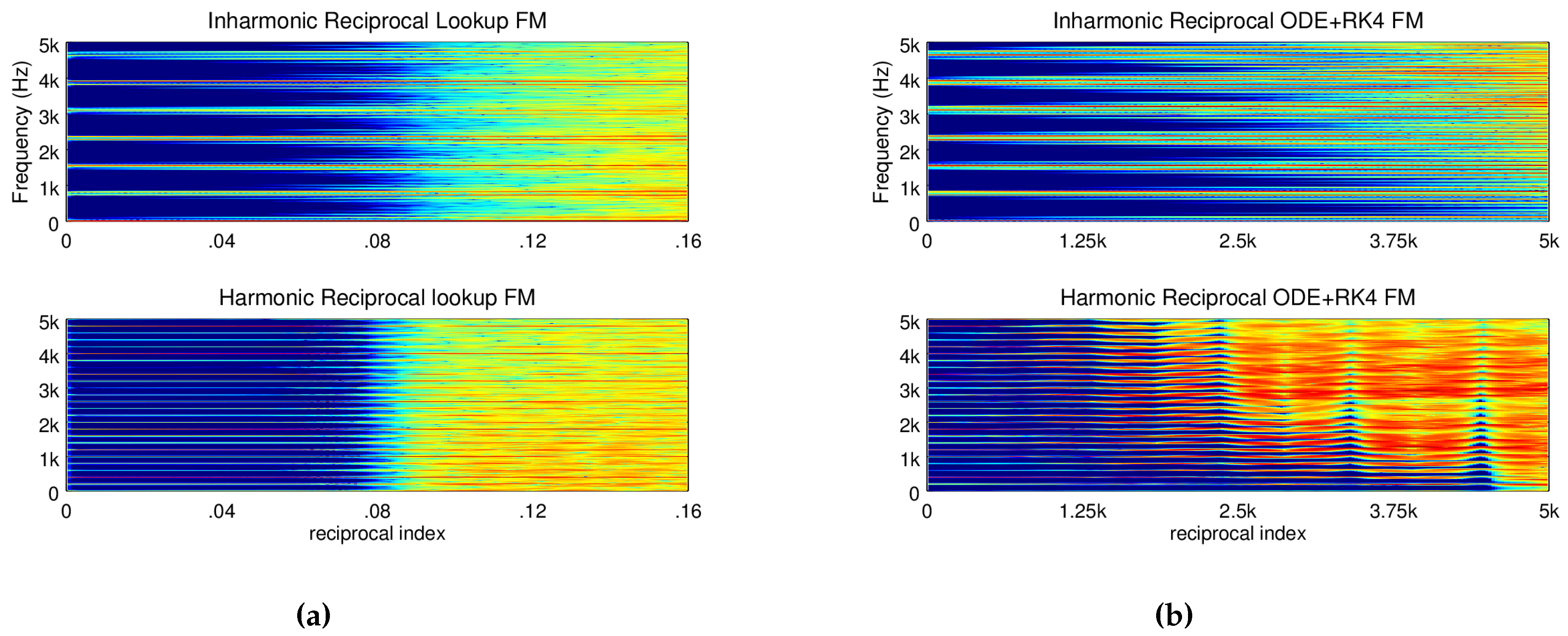
Figure 5a and Figure 5b compare reciprocal FM implemented as ODEs and as lookup oscillators. As the plots show, delay (in this case 0.0208 ms which is 1 sample at 48 kHz) between the lookup oscillators in a reciprocal FM network creates inharmonic distortion that is similar to broadband noise at higher modulation indices. On the contrary the ODE + RK4 implementation produces very different results. Broadband noise does not appear, and in the harmonic case, a low frequency periodicity emerges.
The meaning of the modulation index is very different in the two implementations. The values given in Figure 5 were chosen by ear and by examining magnitude spectra so that they were roughly equivalent. There is a complex and nonlinear relationship between the equivalent indices in the two implementations.
As a final note, feedback FM (FBFM) has been known for some time [26]. FBFM differs from reciprocal FM in that FBFM needs only one lookup oscillator whose delayed output modulates its own phase input signal. As in the case with reciprocal FM, FBFM will cause a great deal of aliasing and foldover at higher indices and this comes across as broadband noise (Figure 6). In the ODE + RK4 implementation of FBFM we instead see that higher modulation indices bring about a flattening effect along with increased harmonic energy.
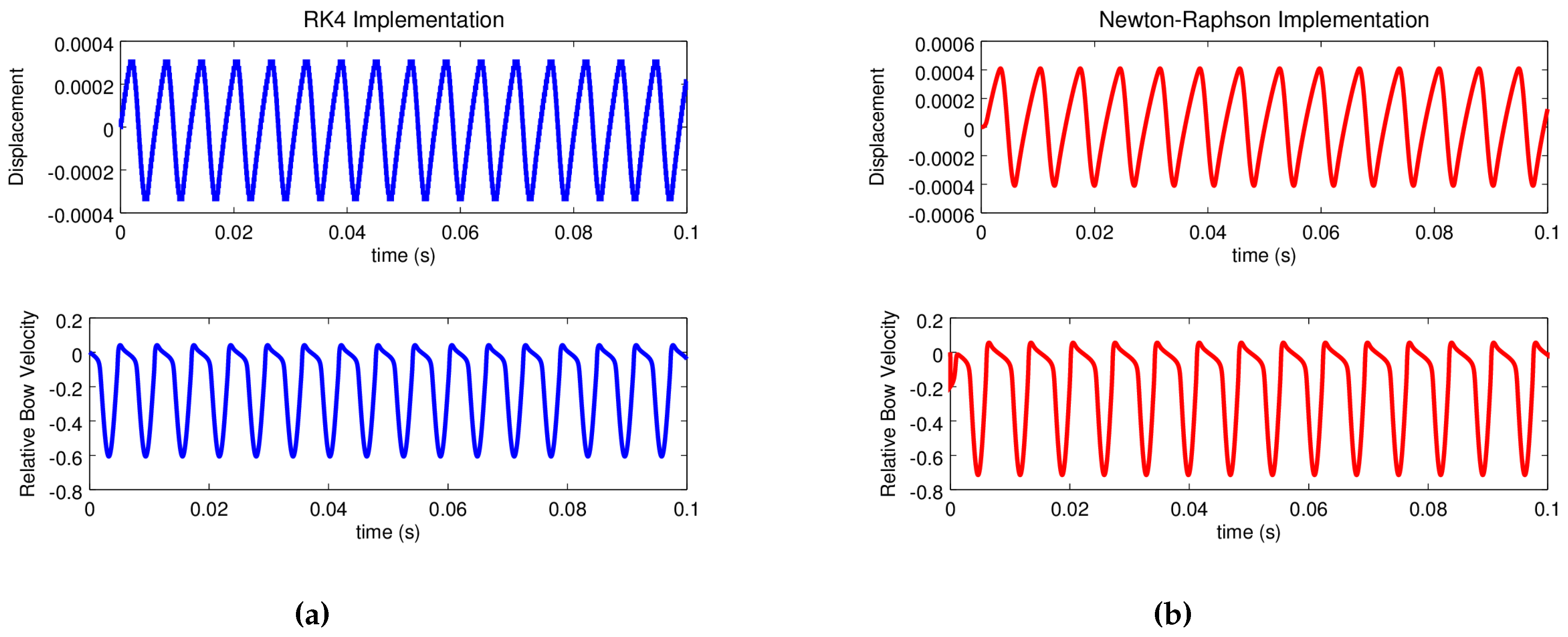
3.4. A Bowed Oscillator
In addition to arranging simple harmonic oscillators in delay-free feedback networks, we may use ODEs and RK4 as a means of introducing physically motivated nonlinearities. As an example, consider a harmonic oscillator driven by friction—such as a point on a bowed violin string.
The physics of bow-string interaction is well understood [27,28,29]. The effect of the bow on the point of bowing is usually modeled through a nonlinear function which is coupled to the point of bowing (here given as a single oscillator). The motion of this oscillator is
In this model u is displacement of the oscillator, is the fundamental frequency, is the force of the bow divided by mass (which is a quantity we neglect to include in our model in favor of using ), v is the oscillator’s velocity, is the velocity of the bow, and Φ is a nonlinear friction model such as:
where a is a coefficient of friction and .
As is the case with the second order spring-mass system given in Equation (11), we can re-write Equation (23) as a pair of ODEs:
and solve with RK4.
A slightly different form of this model is discussed in Chapter 3 of [21]. There, the linear part of Equation (23) is solved with Backward Euler, and the nonlinearity Φ is solved with Newton-Raphson. This requires, of course, that Φ be differentiable and that the derivative be determined prior to computation. Furthermore, Newton-Raphson is an iterative solver so it may not be appropriate for real-time implementation due to convergence issues. These two implementations are compared in Figure 7. The code used to generate the Newton-Raphson version of the system was taken directly from Appendix A in [21].
Since RK4 puts us in a position to solve the system without having to differentiate Φ, we are free to experiment with friction models that are discontinuous. For example, we may study the discontinuous friction model given by
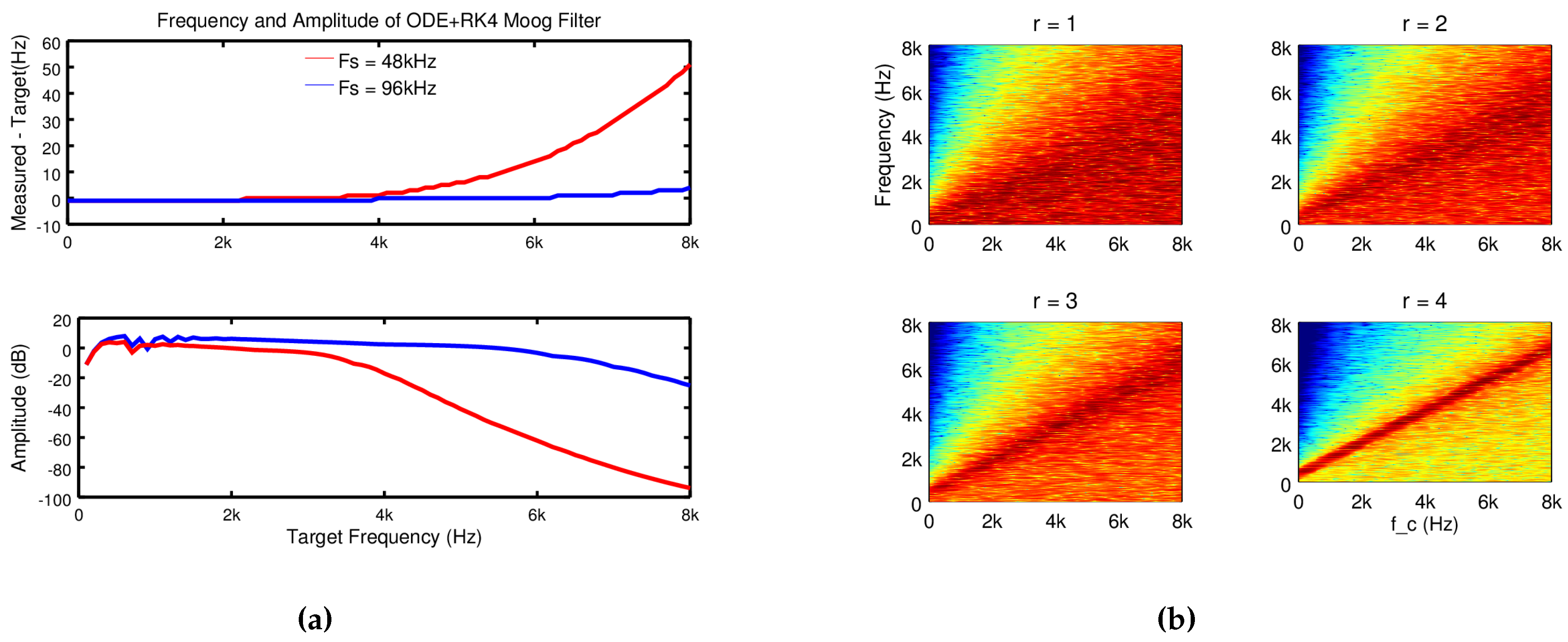
3.5. The Moog Ladder Filter
As an example of a musically interesting application of ODES and RK4 in audio synthesis that is not based on harmonic motion, we return to the ‘ladder filter’ invented by Robert Moog in 1965 [30]. This filter has been subject to numerous studies since [1]. Most digitizations use the bilinear transform [31] or some similar procedure [32] to discretize the linear portion (small signal response) of the analog transfer function. As mentioned above, since there is feedback in the circuit, digitizations of this filter often include unit sample feedback (). Again, this is problematic because the delay couples the gain parameter g (which controls the cutoff frequency of the filter) to the resonance parameter r (which controls the bandwidth of the filter). This causes additional phase shifting so that effect of the resonance parameter varies with frequency and vice versa. Many adjustments have been suggested to ameliorate this artifact of digitization [33] or to avoid the addition of delay to the feedback part of the filter without resorting to iteration. Examples of this include solution through the use of Volterra series [34,35] and linear compensation filters [36].
The Moog ladder filter is a four-pole network, wherein the voltage across each stage is defined:
where r is the gain that governs the cutoff frequency of the filter, is the change in voltage across stage i, is the present voltage across stage i, and is the present voltage across the previous stage for . Ideally, the cutoff frequency has a ratio of Hz for all frequencies.
Since each stage of the filter shifts the input signal phase by radians, the output of the filter is inverted and fed back into the input to create resonance. So, for we have:
when , the filter saturates and will oscillate on its own. In the results presented here, we simply plug Equations (27) and (28) into RK4 and grind out the samples. As indicated by the results, no further analysis, linearization, or digitization than this is necessary to achieve good results.
Figure 9a shows a comparison of measured frequency and amplitude for impulses fed to the filter tuned to various values for the parameter . This compare favorably with the results presented in [32] where compensation for the zero introduced by unit delay in the feedback path results in unbounded amplitude growth at higher values of . The relationship between and the measured frequency peaks in Figure 9b compares favorably with a similar analysis of another delay-free implementation given in [36]. Here there is noticeable flattening that results from lowering the value of r. This suggests that some coupling between this parameter and persists.
4. Discussion
The above results show a small number of possible applications for the explicit solution of dynamical systems in audio synthesis. The benefit of the methods given here (defining a system as a network of ODEs then declaring that system to a software layer that can solve each equation in a time accurate manner) is simply that a user can easily create interesting and desirable sounds without having first to resort to deep analysis prior to synthesis. The drawback is that it cannot solve for implicit relations and that the numerical solver may fail when presented with stiff equations. There is no free lunch. However this method can be harnessed to synthesize implicit systems provided they can be expressed as coupled explicit ODEs. It is likely that by extending known systems that fit these requirements and by inventing new ones, many new interesting musical sounds and behaviors can be defined.
5. Conclusions
We present above a method for getting around (so to speak) the problem of delay-free loops in certain nonlinear digital synthesis routines. We do this by imposing the constraint that the systems we synthesize be ones that can be represented entirely through explicit first order ODEs. Explicit solvers can (more or less accurately) compute the output of each ODE even if there is instantaneous feedback in the network structure. There are many such systems that are of interest and the above shows only a few.
Conflicts of Interest
The author declares no conflict of interest.
References
- Stilson, T.; Smith, J. Analyzing the Moog VCF with considerations for digital implementation. In Proceedings of the 1996 International Computer Music Conference, Hong Kong, China, 19–24 August 1996; pp. 398–401.
- Nagel, L.W.; Pederson, D.O. SPICE: Simulation Program with Integrated Circuit Emphasis; No. UCB/ERL M382; Electronics Research Laboratory, College of Engineering, University of California: Berkeley, CA, USA, 12 April 1973. [Google Scholar]
- Fettweis, A. Digital filters related to classical structures. AEU Arch. Elektron. Ubertragungstechnik 1971, 25, 78–89. [Google Scholar]
- Pakarinen, J.; Tikander, M.; Karjalainen, M. Wave digital modeling of the output chain of a vacuum-tube amplifier. In Proceedings of the International Conference on Digital Audio Effects (DAFx), Como, Italy, 1–4 September 2009; pp. 1–4.
- Pakarinen, J.; Karjalainen, M. Enhanced wave digital triode model for real-time tube amplifier emulation. IEEE Trans. Audio Speech Lang. Process. 2010, 18, 738–746. [Google Scholar] [CrossRef]
- Välimäki, V.; Bilbao, S.; Smith, J.O.; Abel, J.S.; Pakarinen, J.; Berners, D. Virtual Analog Effects. In DAFX: Digital Audio Effects, 2nd ed.; Wiley: Hoboken, NJ, USA, 2011. [Google Scholar]
- Van Duyne, S.A.; Pierce, J.R.; Smith, J.O. Traveling wave implementation of a lossless mode-coupling filter and the wave digital hammer. In Proceedings of the International Computer Music Conference, Aarhus, Denmark, 12–17 September 1994; pp. 411–418.
- Bensa, J.; Bilbao, S.; Martinet, K.R.; Smith, J. A power normalized non-linear lossy piano hammer. In Proceedings of the Stokholm Muisc Acoustics Conference, Stokholm, Sweden, 2–9 August 2003; pp. 365–368.
- Van Walstijn, M.; Campbell, M. Discrete-time modeling of woodwind instrument bores using wave variables. J. Acoust. Soc. Am. 2003, 113, 575–585. [Google Scholar] [CrossRef] [PubMed] [Green Version]
- Borin, G.; de Poli, G.; Rocchesso, D. Elimination of delay-free loops in discrete-time models of nonlinear acoustic systems. IEEE Trans. Speech Audio Process. 2000, 8, 597–605. [Google Scholar] [CrossRef]
- Werner, K.; Nangia, V.; Smith, J., III; Abel, J. Resolving wave digital filters with multiple/multiport nonlinearities. In Proceedings of the Digital Audio Effects (DAFx), Trondheim, Norway, 30 November–3 December 2015.
- Werner, K.; Smith, J., III; Abel, J. Wave digital filter adaptors for arbitrary topologies and multiport linear elements. In Proceedings of the Digital Audio Effects (DAFx), Trondheim, Norway, 30 November–3 December 2015.
- Yeh, D.T.; Abel, J.S.; Smith, J.O., III. Automated physical modeling of nonlinear audio circuits for real-time audio effects—Part I: theoretical development. IEEE Trans. Audio Speech Lang. Process. 2010, 18, 728–737. [Google Scholar] [CrossRef]
- Yeh, D.T. Automated physical modeling of nonlinear audio circuits for real-time audio effects—Part II: BJT and vacuum tube examples. IEEE Trans. Audio Speech Lang. Process. 2012, 20, 1207–1216. [Google Scholar] [CrossRef]
- Dempwolf, K.; Holters, M.; Zölzer, U. Discretization of parametric analog circuits for real-time simulations. In Proceedings of the 13th International Conference on Digital Audio Effects, Graz, Austria, 4–6 September 2010.
- Yeh, D.T.M. Digital Implementation of Musical Distortion Circuits by Analysis and Simulation. Ph.D. Thesis, Stanford University, Stanford, CA, USA, June 2009. [Google Scholar]
- Puckette, M. Pure Data: Another integrated computer music environment. In Proceedings of the Second Intercollege Computer Music Concerts, Tachikawa, Japan, 7 May 1997; pp. 37–41.
- Medine, D. Unsampled Digitial Synthesis: Computing the Output of Implicit and Non-Linear Systems. In Proceedings of the International Computer Music Conference, Denton, TX, USA, 25 September–1 October 2015; pp. 90–93.
- Yeh, D.T.; Abel, J.; Smith, J.O. Simulation of the diode limiter in guitar distortion circuits by numerical solution of ordinary differential equations. In Proceedings of the 10th International Conference on Digital Audio Effects, Bordeaux, France, 10–15 September 2007; pp. 197–204.
- Macak, J.; Schimmel, J. Nonlinear circuit simulation using time-variant filter. In Proceedings of the International Conference on Digital Audio Effects (DAFx), Como, Italy, 1–4 September 2009.
- Bilbao, S. Numerical Sound Synthesis: Finite Difference Schemes and Simulation in Musical Acoustics; Wiley Online Library: Hoboken, NJ, USA, 2009. [Google Scholar]
- Mathews, M.; Smith, J.O. Methods for synthesizing very high Q parametrically well behaved two pole filters. In Proceedings of the Stockholm Musical Acoustics Conference (SMAC), Stockholm, Sweden, 6–9 August 2003.
- Puckette, M. The Theory and Technique of Electronic Music; World Scientific: Singapore, 2007. [Google Scholar]
- Chowning, J.M. The synthesis of complex audio spectra by means of frequency modulation. J. Audio Eng. Soc. 1973, 21, 526–534. [Google Scholar]
- Chowning, J.M. Method of synthesizing a musical sound. US Patent 4,018,121, April 1977. [Google Scholar]
- Tomisawa, N. Tone production method for an electronic musical instrument. US Patent 4,249,447, February 1981. [Google Scholar]
- McIntyre, M.; Woodhouse, J. On the fundamentals of bowed-string dynamics. Acta Acust. United Acust. 1979, 43, 93–108. [Google Scholar]
- Cremer, L.; Allen, J.S. The Physics of the Violin; MIT Press: Cambridge, MA, USA, 1984. [Google Scholar]
- Serafin, S. The Sound of Friction: Real-time Models, Playability and Musical Applications. Ph.D. Thesis, Stanford University, Stanford, CA, USA, June 2004. [Google Scholar]
- Moog, R.A. A voltage-controlled low-pass high-pass filter for audio signal processing. In Proceedings of the 17th Audio Engineering Society Convention, New York, NY, USA, 11–15 October 1965.
- D’Angelo, S.; Valimaki, V. An improved virtual analog model of the Moog ladder filter. In Proceedings of the 2013 IEEE International Conference on Acoustics, Speech and Signal Processing, Vancouver, BC, Canada, 26–31 May 2013; pp. 729–733.
- Huovilainen, A. Nonlinear digital implementation of the Moog ladder filter. In Proceedings of the International Conference on Digital Audio Effects (DAFx), Naples, Italy, 5–8 October 2004; pp. 61–64.
- Daly, P. A Comparison of Virtual Analogue Moog VCF Models. Master’s Thesis, University of Edinburgh, Edinburgh, UK, August 2012. [Google Scholar]
- Hélie, T. On the use of Volterra series for real-time simulations of weakly nonlinear analog audio devices: Application to the Moog ladder filter. In Proceedings of the International Conference on Digital Audio Effects (DAFx), Montreal, QC, Canada, 18–20 September 2006; pp. 7–12.
- Hélie, T. Volterra series and state transformation for real-time simulations of audio circuits including saturations: Application to the Moog ladder filter. IEEE Trans. Audio Speech Lang. Process. 2010, 18, 747–759. [Google Scholar] [CrossRef]
- D’Angelo, S.; Valimaki, V. Generalized Moog ladder filter: Part II–Explicit nonlinear model through a novel delay-free loop implementation method. IEEE/ACM Trans. Audio Speech. Lang. Process. 2014, 22, 1873–1883. [Google Scholar] [CrossRef]
Figure 1.
Continuous-time (a) and discrete time (b) block diagrams of the Moog ladder filter after Stilson and Smith, 1996 [1].
Figure 1.
Continuous-time (a) and discrete time (b) block diagrams of the Moog ladder filter after Stilson and Smith, 1996 [1].

Figure 2.
Block diagrams showing the signal flow for reciprocal sync. Using dyamical oscillators. (a) Using lookup oscillators; (b) Using dyamical oscillators.
Figure 2.
Block diagrams showing the signal flow for reciprocal sync. Using dyamical oscillators. (a) Using lookup oscillators; (b) Using dyamical oscillators.

Figure 3.
The output of (a) two digital lookup oscillators in a tight sync loop and (b) another pair given Equations (16) and (17) fed to the fourth order Runge-Kutta (RK4) method for solution. (a) 950 Hz and 900 Hz digital lookup oscillators in reciprocal sync. ; (b) The same parameters but using the dynamical model in Equations (16) and (17).

Figure 4.
Signal flow diagram for a reciprocal frequency modulation (FM) scheme without delay.
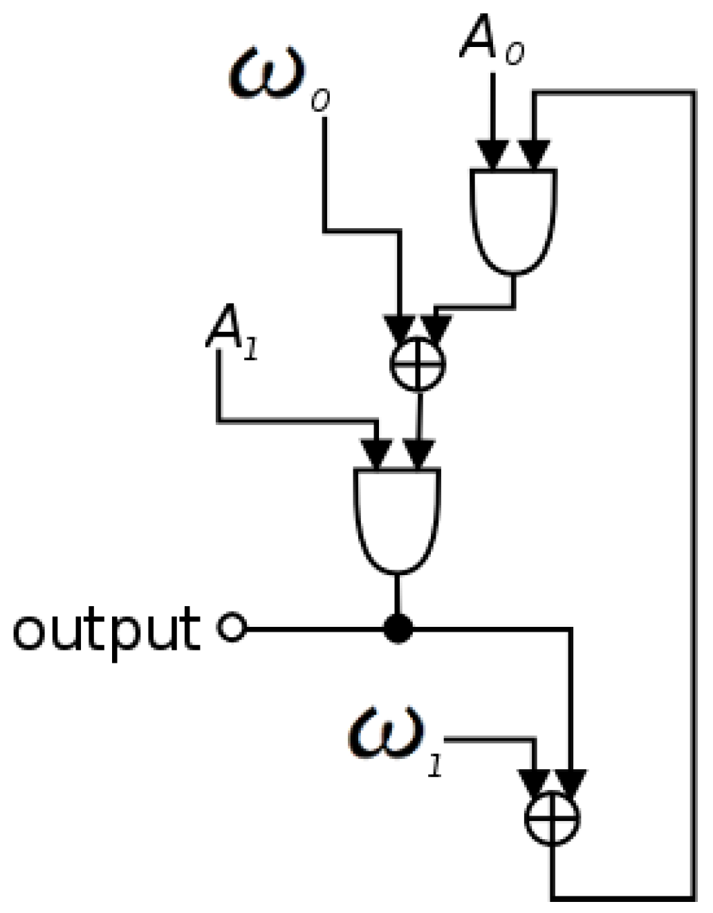
Figure 5.
Spectrograms of (a) reciprocal frequency modulation using lookup oscillators of frequencies 800 Hz and 777 Hz in the top and 800 Hz and 600 Hz in the bottom; In (b) the same network with the same frequencies, but using the ODE (ordinary differential equation) + RK4 implementation. In all four plots the modulation index of the 800 Hz oscillator is held fixed while the other modulation index is swept upwards

Figure 6.
Sweeping the modulation index in feedback FM.

Figure 7.
The bowed oscillator model given here (solved with RK4) and that given in [21]. In both implementations, oscillator frequency , , and . (a) The system given in Equation (25) solved using RK4; (b) Using Newton-Raphson and Backward Euler to solve Equation (23).

Figure 8.
RK4 solving Equations (25) using (a) the continuous friction model in Equation (24) and (b) Equation (26). (a) Differentiable friction model; (b) Discontinuous friction model.
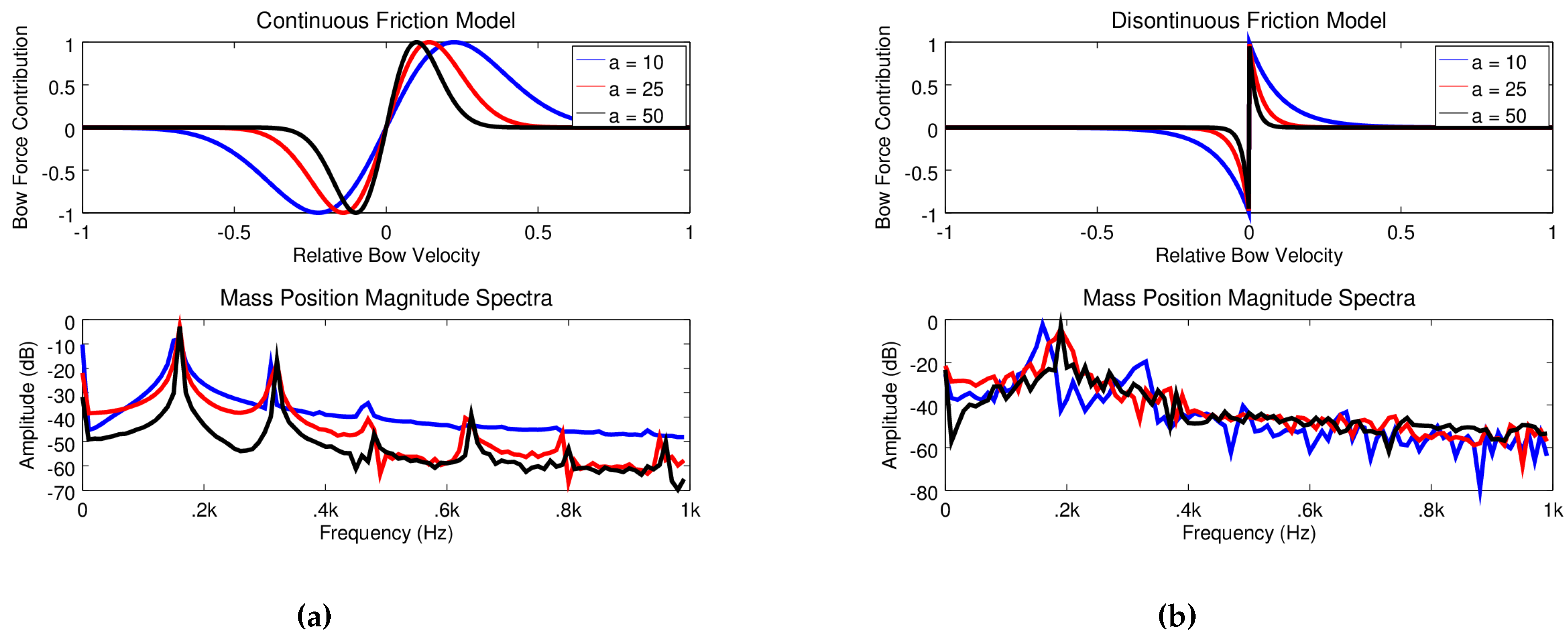
Figure 9.
Plots illustrating the character of the ODE + RK4 implementation of the Moog filter. (a) Shown is the difference between target frequency and highest peak in the spectrum as well as amplitude for the ODE + RK4 Moog filter; (b) Sweeping across a noise stimulated Moog filter for various values of (sampling rate is 48 kHz).

© 2016 by the author; licensee MDPI, Basel, Switzerland. This article is an open access article distributed under the terms and conditions of the Creative Commons Attribution (CC-BY) license (http://creativecommons.org/licenses/by/4.0/).
Share and Cite
MDPI and ACS Style
Medine, D. Dynamical Systems for Audio Synthesis: Embracing Nonlinearities and Delay-Free Loops. Appl. Sci. 2016, 6, 134. https://doi.org/10.3390/app6050134
AMA Style
Medine D. Dynamical Systems for Audio Synthesis: Embracing Nonlinearities and Delay-Free Loops. Applied Sciences. 2016; 6(5):134. https://doi.org/10.3390/app6050134
Chicago/Turabian StyleMedine, David. 2016. "Dynamical Systems for Audio Synthesis: Embracing Nonlinearities and Delay-Free Loops" Applied Sciences 6, no. 5: 134. https://doi.org/10.3390/app6050134
Note that from the first issue of 2016, this journal uses article numbers instead of page numbers. See further details here.