Psychoacoustic Approaches for Harmonic Music Mixing ^†

Abstract

The practice of harmonic mixing is a technique used by DJs for the beat-synchronous and harmonic alignment of two or more pieces of music. In this paper, we present a new harmonic mixing method based on psychoacoustic principles. Unlike existing commercial DJ-mixing software, which determines compatible matches between songs via key estimation and harmonic relationships in the circle of fifths, our approach is built around the measurement of musical consonance. Given two tracks, we first extract a set of partials using a sinusoidal model and average this information over sixteenth note temporal frames. By scaling the partials of one track over ±6 semitones (in 1/8th semitone steps), we determine the pitch-shift that maximizes the consonance of the resulting mix. For this, we measure the consonance between all combinations of dyads within each frame according to psychoacoustic models of roughness and pitch commonality. To evaluate our method, we conducted a listening test where short musical excerpts were mixed together under different pitch shifts and rated according to consonance and pleasantness. Results demonstrate that sensory roughness computed from a small number of partials in each of the musical audio signals constitutes a reliable indicator to yield maximum perceptual consonance and pleasantness ratings by musically-trained listeners.

1. Introduction

The digital era of DJ-mixing has opened up DJing to a huge range of users and has also enabled new technical possibilities in music creation and remixing. The industry-leading DJ-software tools now offer users of all technical abilities the opportunity to rapidly and easily create DJ mixes out of their personal music collections or those stored online. Central to these DJ-software tools is the ability to robustly identify tempo and beat locations, which, when combined with high quality audio time-stretching, allow for automatic “beat-matching” (i.e., temporal synchronization) of music [1].

In addition to leveraging knowledge of the beat structure, these tools also extract harmonic information, typically in the form of an estimated key. Knowing the key of different pieces of music allows users to engage in so-called “harmonic mixing”, where the aim is not only to align music in time, but also in key. Different pieces of music are deemed to be harmonically compatible if their keys exactly match or adhere to well-known relationships within the circle of fifths, e.g., those in relative keys (major and relative minor) or those separated by a perfect fourth or perfect fifth occupying adjacent positions [2]. When this information is combined with audio pitch-shifting (i.e., the ability to transpose a piece of music by some number of semitones independently of its temporal structure), it provides a seemingly powerful means to “force” the harmonic alignment between two pieces of otherwise harmonically incompatible music in the same way beat matching works for the temporal dimension [3]. To illustrate this process by example, consider two musical excerpts, one in D minor and the other in F minor. Since both excerpts are in a minor key, the key-based match can be made by simply transposing the second down by three semitones. Alternatively, if one excerpt is in A major and the other is in G# minor, this would require pitch shifting the second excerpt down by two semitones to F# minor, which is the relative minor of A major.

While the use of tempo and key detection along with high quality music signal processing techniques is certainly effective within specific musical contexts, in particular for harmonically- and temporally-stable house music (and other related genres), we believe the key-based matching approach has several important limitations. Perhaps the most immediate of these limitations is that the underlying key estimation might be error-prone, and any errors would then propagate into the harmonic mixing. In addition to this, a global property, such as musical key, provides almost no information regarding what is in the signal itself and, in turn, how this might affect perceptual harmonic compatibility for listeners when two pieces are mixed. Similarly, music matching based on key alone provides no obvious means for ranking the compatibility, and hence, choosing, among several different pieces of the same key [3]. Likewise, assigning one key for the duration of a piece of music cannot indicate where in time the best possible mixes (or mashups) between different pieces of music might occur. Even with the ability to use pitch-shifting to transpose the musical key, it is important to consider the quantization effect of only comparing whole semitone shifts. The failure to consider fine-scale tuning could lead to highly dissonant mistuned mixes between songs that still share the same key.

Towards overcoming some of the limitations of key-based mixing, beat-synchronous chromagrams [3,4] have been used as the basis for harmonic alignment between pieces of music. However, while the chromagram provides a richer representation of the input signal than using key alone, it nevertheless relies on the quantization into discrete pitch classes and the folding of all harmonic information into a single octave to faithfully represent the input. In addition, harmonic similarity is used as a proxy for harmonic compatibility.

Therefore, to fully address the limitations of key-based harmonic mixing, we propose a new approach based on the analysis of consonance. We base our approach on the well-established psychoacoustic principles of sensory consonance and harmony as defined by Ernst Terhardt [5,6], where our goal is to discover the optimal, consonance-maximizing alignment between two music excerpts. In this way, we avoid looking for harmonic similarity and seek to move towards a direct measurement of harmonic compatibility. To this end, we first extract a set of frequencies and amplitudes using a sinusoidal model and average this information over short temporal frames. We fix the partials of one excerpt and apply a logarithmic scaling to the partials of the other over a range of one full octave in 1/8th semitone steps. Through an exhaustive search, we can identify the frequency shift that maximizes the consonance between the two excerpts and then apply the appropriate pitch-shifting factor prior to mixing the two excerpts together. A graphical overview of our approach is given in Figure 1.

Searching across a wide frequency range in small steps allows both for multiple possible harmonic alignments and the ability to compensate for differences in tuning. In comparison with an existing commercial DJ-mixing system, we demonstrate that our approach is able to provide mixes that were considered significantly both more consonant and more pleasant by musically-trained listeners.

In comparison to our previous work [7], the main contribution of this paper relates to an extended evaluation. To this end, we largely maintain the original description of our original method, but we provide the results of a new listening test, a more detailed statistical analysis and an examination of the effect of the parameterization of our model.

The remainder of this paper is structured as follows. In Section 2, we review existing approaches for the measurement of consonance based on roughness and pitch commonality. In Section 3, we describe our approach for consonance-based music mixing driven by these models. We then address the evaluation of our approach in Section 4 via a listening test and explore the effect of the parameterization of our model. Finally, in Section 5, we present conclusions and areas for future work.

2. Consonance Models

In this section, we present the theoretical approaches for the computational estimation of consonance that will form the core of the overall implementation described in Section 3 for estimating the most consonant combination of two tracks. To avoid misunderstandings due to ambiguous terminology, we define consonance by means of Terhardt’s psychoacoustic model [5,6], which is divided into two categories: The first, sensory consonance, combines roughness (and fluctuations, standing for slow beatings and therefore equated with roughness throughout), sharpness (referring to high energy in high registers of a sound’s timbre) and tonalness (the degree of tonal components a sound holds). The second, harmony, is mostly built upon Terhardt’s virtual pitch theory, which describes the effect of perceiving an imaginary root pitch of a sonority’s harmonic pattern. This, in terms of musical consonance, he calls the root relationship, whereas he describes pitch commonality as the degree of how similar the harmonic patterns of two sonorities are. We take these categories as the basis for our approach. To estimate the degree of sensory consonance, we use a modified version of Hutchinson and Knopoff’s [8] roughness model. For calculating the pitch commonality of a combination of sonorities, we propose a model that combines Parncutt’s [9] pitch categorization procedure with Hofmann-Engl’s [10] virtual pitch and chord similarity model. Both models take a sequence of sinusoids, expressed as frequencies, $f_i$ in Hz, and amplitudes, $M_i$ in dBSPL (sound pressure level), as input.

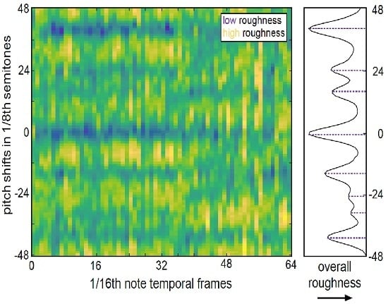
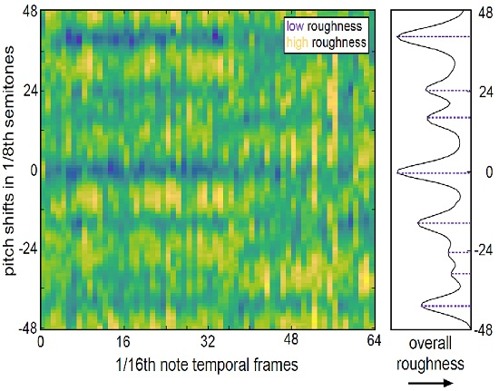
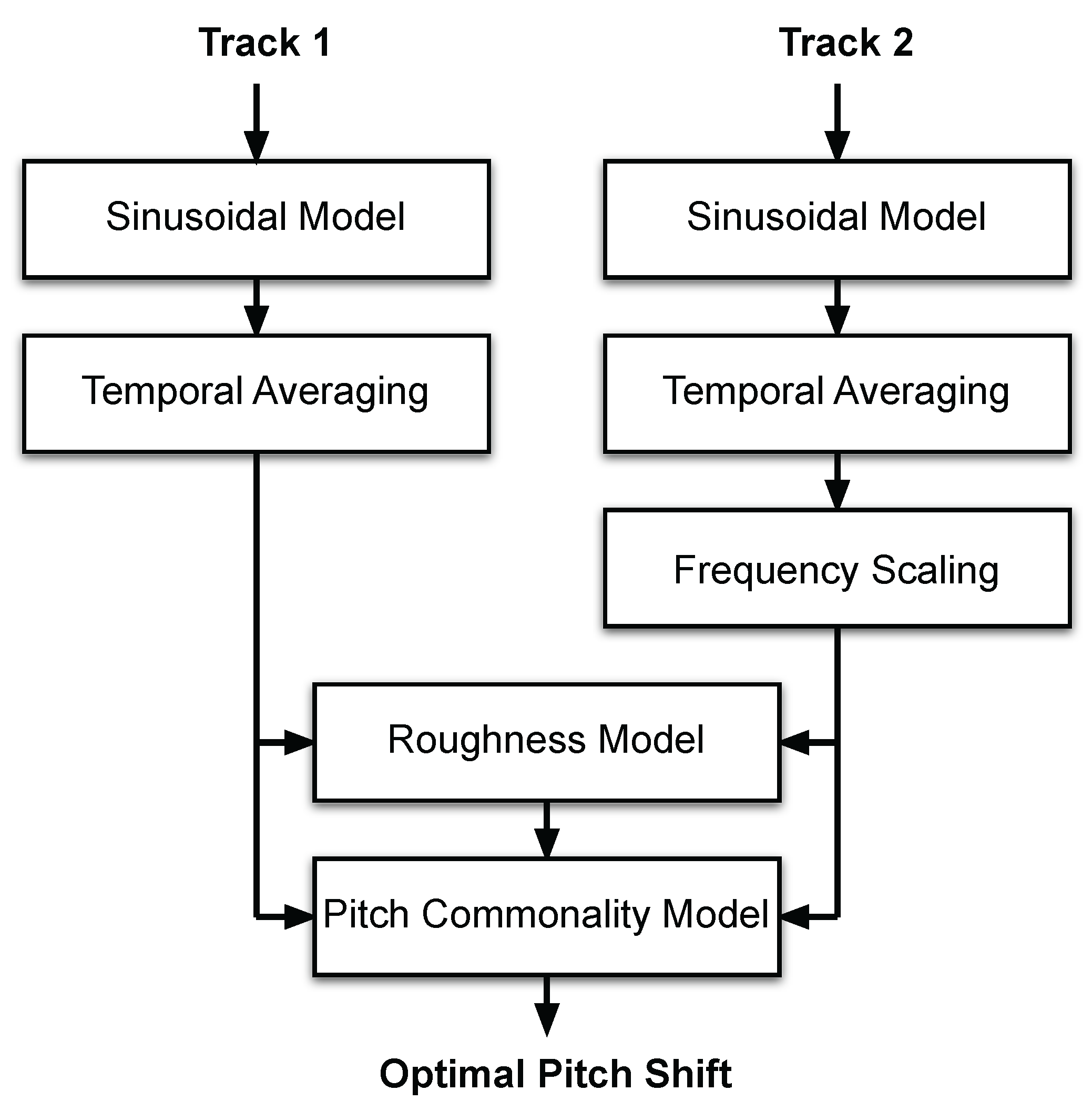
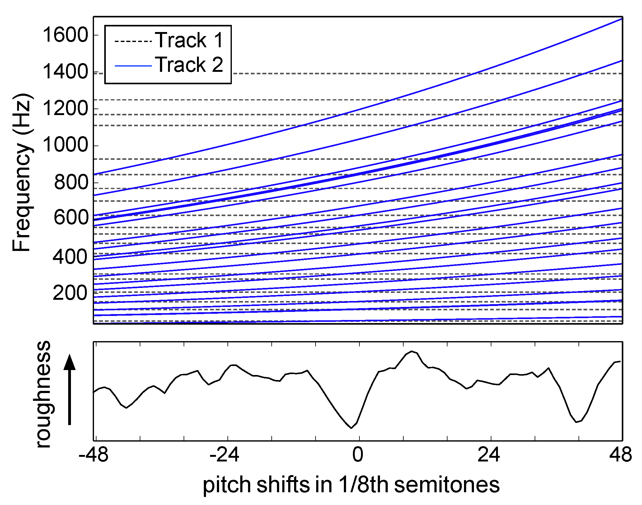
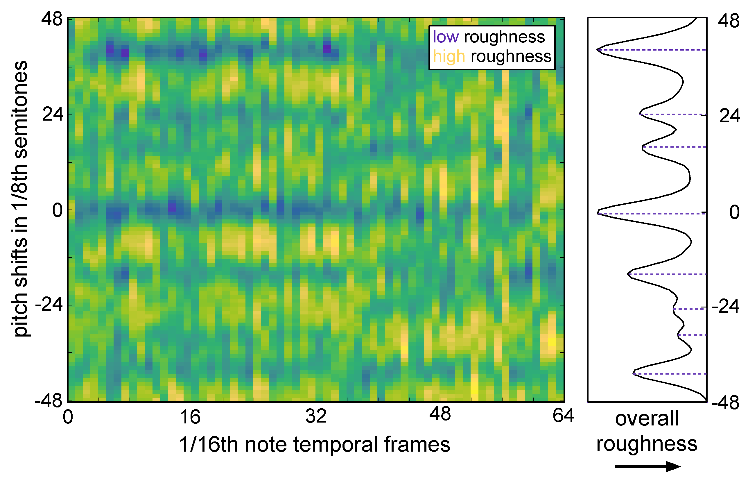
2.1. Roughness Model

As stated above, the category of sensory consonance can be divided into three parts: roughness, tonalness and sharpness. While sharpness is closely connected to the timbral properties of musical audio [6], we do not attempt to model or modify this aspect, since it can be considered independent of the interaction of two pieces of music, which is the object of our investigation in this paper. Parncutt and Strasburger [11] discuss the strong relationship between roughness and tonalness as a sufficient reason to only analyze one of the two properties. The fact that roughness has been more extensively explored than tonalness and that most sensory consonance models build exclusively upon it motivates the use of roughness as our sole descriptor for sensory consonance in this work. For each of the partials of a spectrum, the roughness that is evoked by the co-occurrence with other partials is computed, then weighted by the dyads’ amplitudes and, finally, summed for every sinusoid.

The basic structure of this procedure is a modified version of Hutchinson and Knopoff’s [12] roughness model for complex sonorities that builds on the roughness curve for pure tone sonorities proposed by Plomp and Levelt [13] (this approach also forms the basis of work by Sethares [14] and Bañuelos [15] on the analysis of consonance in tuning systems and musical performance, respectively). A function that approximates the graph estimated by Plomp and Levelt is proposed by Parncutt [16]:

$$g(y)=\left\{\begin{array}{cc}{(exp(1)\frac{y}{0.25}exp(-\frac{y}{0.25}))}^2\hfill & y<1.2\\ 0\hfill & \mathrm{otherwise}\end{array}\right.$$

(1)

where $g(y)$ is the degree of roughness of a dyad and y the frequency interval between two partials ($f_i$ and $f_j$) expressed in the critical bandwidth ($\mathrm{CBW}$) of the mean frequency $\overline{f}$, such that:

$$y=\frac{|f_j-f_i|}{\mathrm{CBW}(\overline{f})}$$

(2)

and:

$$\overline{f}=\frac{f_i+f_j}{2}.$$

(3)

Since pitch perception is based on ratios, we substitute $\mathrm{CBW}(\overline{f})$ with Moore and Glasberg’s [17] equation for the equivalent rectangular bandwidth $\mathrm{ERB}(\overline{f})$ in Equation (2).

$$\mathrm{ERB}(\overline{f})=6.23{({10}^{-3}\overline{f})}^2+93.39({10}^{-3}\overline{f})+28.52$$

(4)

which Parncutt [16] also cites as offering “possible minor improvements.” The roughness values $g(y)$ for every dyad are then weighted by the dyad’s amplitudes ($M_i$ and $M_j$) to obtain a value of the overall roughness D of a complex sonority with N partials:

$$D=\frac{{\sum }_{i=1}^N{\sum }_{j=i+1}^N{M}_i{M}_j{g}_{ij}}{{\sum }_{i=1}^N{M}_i^2}.$$

(5)

2.2. Pitch Commonality Model

As opposed to sensory consonance, which can be applied to any arbitrary sound, the second category of Terhardt’s consonance model [5,6] is largely specified on musical sounds. This is why the incorporation of an aspect based on harmony should be of critical importance in a system that aligns music according to consonance. Nevertheless, the analysis of audio with a harmonic model of consonance is currently under-explored in the literature. Existing consonance-based tools for music typically focus on roughness alone [14,18,19]. Relevant approaches that include harmonic analysis perform note extraction, categorization in an octave-ranged chromagram and, as a consequence of this, key detection, but the psychoacoustic aspect of harmony is rarely applied. One of our main aims in this work is therefore to use the existing theoretical background to develop a model that estimates the consonance in terms of root relationship and pitch commonality and ultimately to combine this with a roughness model.

The fundament of the approach lies in harmonic patterns in the spectrum. The extraction of these patterns is taken from the pre-processing stage of the pitch categorization procedure of Parncutt’s model for the computational analysis of harmonic structure [9,11].

For a given set of partials, the audibilities of pitch categories in semitone intervals are produced. Since this corresponds directly to the notes of the chromatic scale, the degree of audibility for different pitch categories can be attributed to a chord. Hofmann-Engl’s [10] virtual pitch model then will be used to compute the “Hofmann-Engl pitch sets” of these chords, which will be subsequently compared for their commonality.

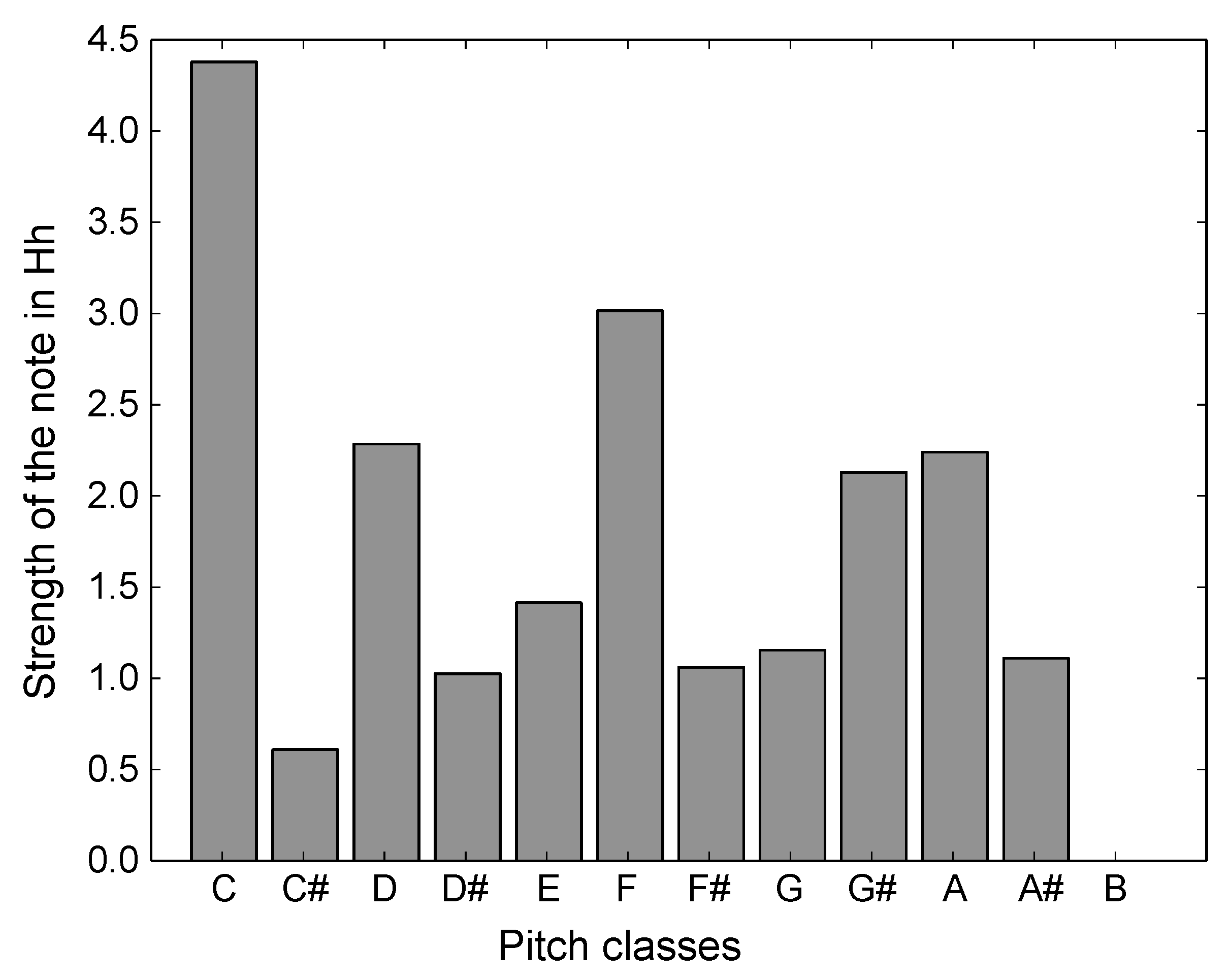
2.2.1. Pitch Categorization

Parncutt’s algorithm detects the particular audibilities for each pure tone, considering the frequency-specific threshold of hearing, masking effects and the theory of virtual pitch. Following Terhardt [20], the threshold in quiet $L_{TH}$ is formulated as:

$$L_{TH}=3.64{f_i}^{-0.8}-6.5exp(-0.6{(f_i-3.3)}^2)+{10}^{-3}{f_i}^4.$$

(6)

Next, the auditory level $\mathsf{{\rm Y}}L$ of a pure tone with its specific frequency $f_i$ is defined as its level in dB above its threshold in quiet,

$$\mathsf{{\rm Y}}L(f_i)=max(0,M_i-L_{TH}(f_i))$$

(7)

Masking depends on the distance of pure tones in critical bandwidths. To simulate the effects of masking in the model, the pitch of the pure tone is examined on a scale that corresponds to critical bandwidths. To this end, the pure tone height, $H_p(f_i)$, for every pitch category, $f_i$, in the spectrum is computed, using the analytic formula by Moore and Glasberg [17] that expresses the critical band rate in ERB (equivalent rectangular bandwidth):

$$H_p(f_i)=H_1{log}_e(\frac{f_i+f_1}{f_i+f_2})+H_0.$$

(8)

As parameters, Moore and Glasberg propose $H_1$ = 11.17 ERB, $H_0$ = 43.0 ERB, $f_1$ = 312 Hz and $f_2$ = 14,675 Hz.

The partial masking level $ml(f_i,f_j)$, which is the degree of how much every pure tone in the sonority with the frequency $f_i$ is masked by an adjacent pure tone with its specific frequency $f_j$ and auditory level $\mathsf{{\rm Y}}L(f_j)$, is estimated as:

$$ml(f_i,f_j)=\mathsf{{\rm Y}}L(f_j)-k_m|H_p(f_j)-H_p(f_i)|$$

(9)

where $k_m$ can take values between 12 and 18 dB (chosen value: 12 dB). The partial masking level is specified in dB. The overall masking level, $ML(f_i)$, of every pure tone is obtained by summing its partial masking levels, which are converted first to amplitudes and, then, after the addition, back to dB levels:

$$ML(f_i)=max(0,(20{log}_{10}\sum _{P\ne P^{\prime }}{10}^{(ml(f_i,f_j)/20)})).$$

(10)

In the case of a pure tone with frequency $f_i$ that is not masked, $ml(f_i,f_j)$ will take a large negative value. This negative value for $ML(f_i)$ is avoided by the use of the max operator when comparing the calculated value to zero.

Following this procedure for each component, we can now obtain its audible level $AL(f_i)$ by subtracting its overall masking level from its auditory level $\mathsf{{\rm Y}}L(f_i)$:

$$AL(f_i)=max(0,(\mathsf{{\rm Y}}L(f_i)-ML(f_i))).$$

(11)

To incorporate the saturation of each pure tone with increasing audible level, the audibility $A_p(f_i)$ is estimated for each pure tone component:

$$A_p(f_i)=1-exp(\frac{-AL(f_i)}{A{L}_0}).$$

(12)

where, following Hesse [21], $A{L}_0$ is set to 15 dB. Due to the need to extract harmonic patterns and to consider virtual pitches, the still audible partials are now assigned discrete semitone values. To this end, frequency values that fall into a certain interval are assigned to so-called pitch categories, P, which are defined by their center frequencies in Hz:

$$P(f_i)=12{log}_2(\frac{f_i}{440})+57$$

(13)

where the standard pitch of 440 Hz (musical note $A_4$) is represented by Pitch Category 57.

For the detection of harmonic patterns in the sonority, a template is used to detect partials of harmonic complex tones shifted over the spectrum in a step size of one pitch category. One pattern’s element is given by the formula:

$$P_n=P_1+⌊12{log}_2(n)+0.5⌋$$

(14)

where $P_1$ represents the pitch category of the lowest element (corresponding to the fundamental) and $P_n$ the pitch category of the n-th harmonic.

Wherever there is a match between the template and the spectrum for each semitone-shift, a complex-tone audibility $A_c(P_1)$ is assigned to the template’s fundamental. To take the lower audibility of higher harmonics into account, they are weighted by their harmonic number, n:

$$A_c(P_1)=\frac{1}{k_T}{\left(\sum _n\sqrt{\frac{A_p(P_n)}{n}}\right)}^2.$$

(15)

where the free parameter $k_T$ is set to three. To estimate the audibility, $A(P)$, of a component that considers both the spectral- and complex-tone audibility of every category, the overall maximum of the two is taken as the general audibility. This choice is supported by Terhardt et al. [20], who state that only either a pure or a complex tone can be perceived at once:

$$A(P)=max(A_p(P),A_c(P)).$$

(16)

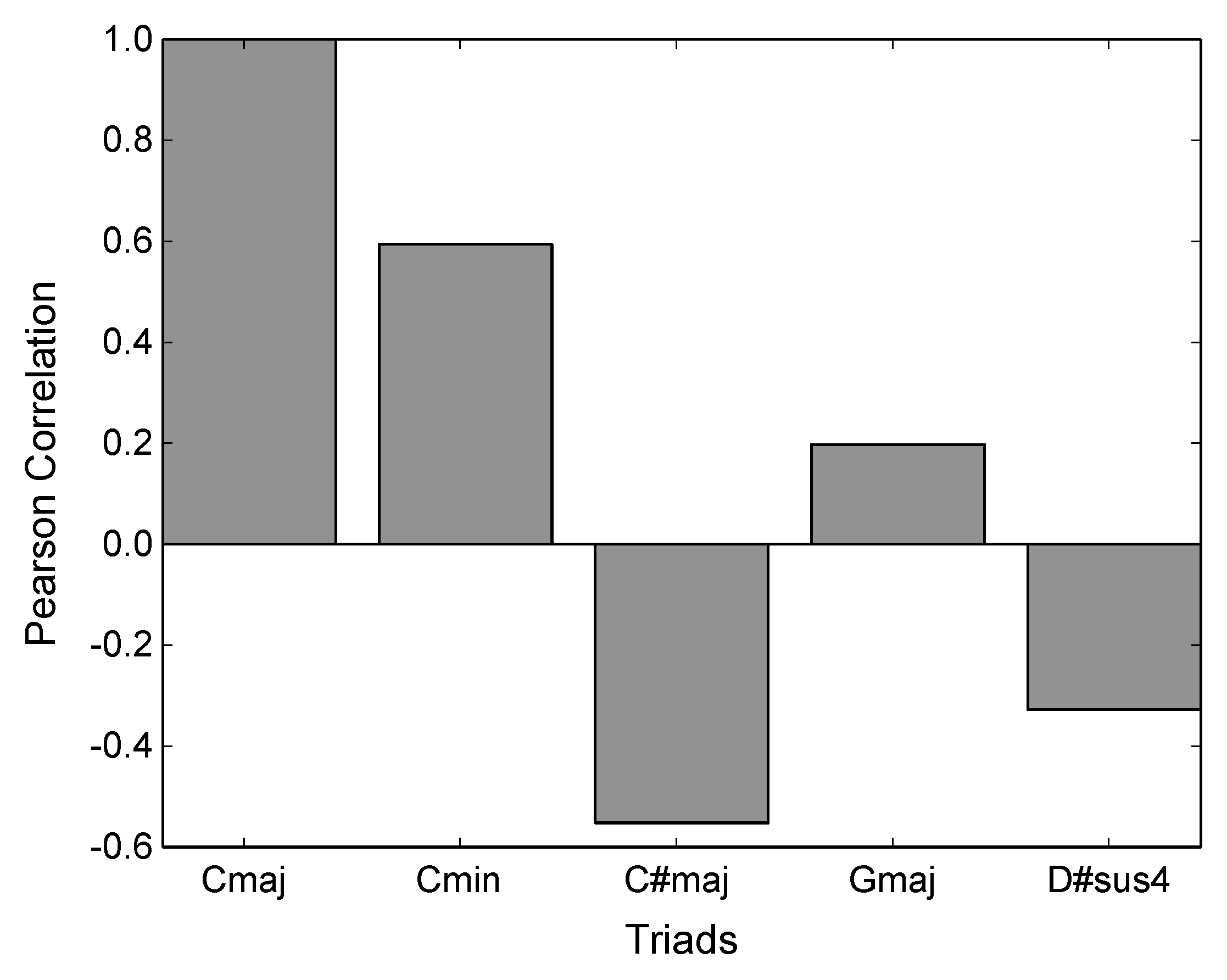
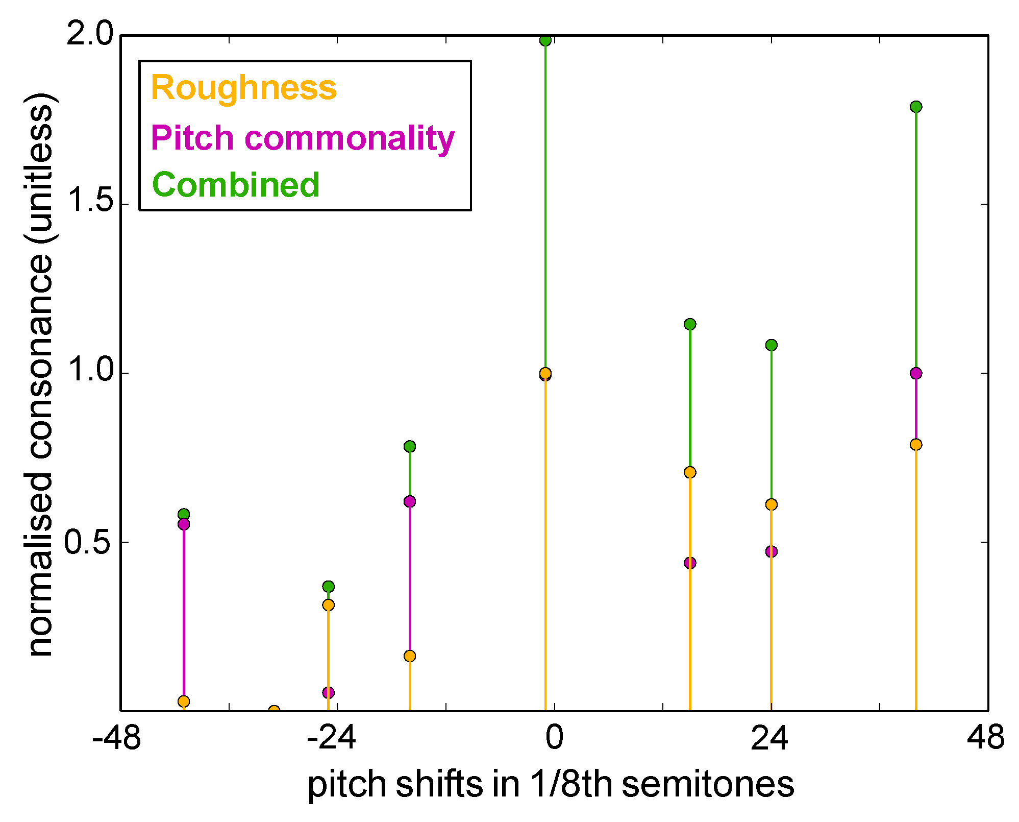
2.2.2. Pitch-Set Commonality and Harmonic Consonance

The resulting set of pitch categories can be interpreted as a chord with each pitch category’s note sounding according to its audibility $A(P)$. With the focus on music and given the importance of the triad in Western culture [22], we extract the three notes of the sonority with the highest audibility.

To compare two chords according to their pitch commonality, Hofmann-Engl proposes to estimate their similarity by the aid of the pitch sets that are produced by his virtual pitch model [23]. The obtained triad is first inserted into a table similar to the one Terhardt uses to analyze a chord for its root note (see [6]), with the exception that Hofmann-Engl’s table contains one additional subharmonic. The notes are ordered from low to high along with their corresponding different subharmonics. A major difference to Terhardt’s model is the introduction of two weights $w_1$ and $w_2$ to estimate the strength ${\beta }_{note}$ for a specific note to be the root of the chord with $Q=3$ tones for all 12 notes of an octave:

$${\beta }_{\mathrm{note}}=\frac{{\sum }_{q=1}^Q{w}_{1,\mathrm{note}}{w}_{2,q}}{Q}$$

(17)

where the result is a set of 12 strengths of notes or so-called “Hofmann-Engl pitches” [23]. As an example, the pitch set deriving from a C major triad is shown in Figure 2. The fusion weight, $w_{1,note}$, is based on note similarity and gives the subharmonics more impact in decreasing order. This implies that the unison and the octave have the highest weight, then the fifth, the major third, and so on. The maximum value of $w_{1,note}$ is c = 6 Hh (Helmholtz; unit set by Hofmann-Engl). The fusion weight is decreased by the variable b, which is b = 1 Hh for the fifth, b = 2 Hh for the major third, b = 3 Hh for the minor seventh, b = 4 Hh for the major second and b = 5 Hh for the major seventh. All other intervals take the value b = 6 and are therefore weighted zero, according to the formula:

$$w_{1,note}=\frac{c^2-b^2}{c}.$$

(18)

The weight according to pitch order, $w_2$, adds greater importance to lower notes, assuming that a lower note is more likely to be perceived as the root of the chord than a higher one and is calculated as:

$$w_{2,q}=\sqrt{\frac{1}{q}}$$

(19)

where q represents the position of the note in the chord. For the comparison between two sonorities (e.g., from different tracks), the Pearson correlation $r_{{\mathrm{set}}_1{\mathrm{set}}_2}$ is calculated for the pair of Hofmann-Engl pitch sets, as Hofmann-Engl [23] proposes to determine chord similarity and, therefore, consonance, C, in the sense of harmony as:

$$C=r_{{\mathrm{set}}_1{\mathrm{set}}_2}.$$

(20)

A graphical example showing the harmonic consonance for different triads compared to the C major triad is shown in Figure 3.

3. Consonance-Based Mixing

Based on the models of roughness and pitch commonality presented in the previous section, we now describe our approach for consonance-based mixing between two pieces of music.

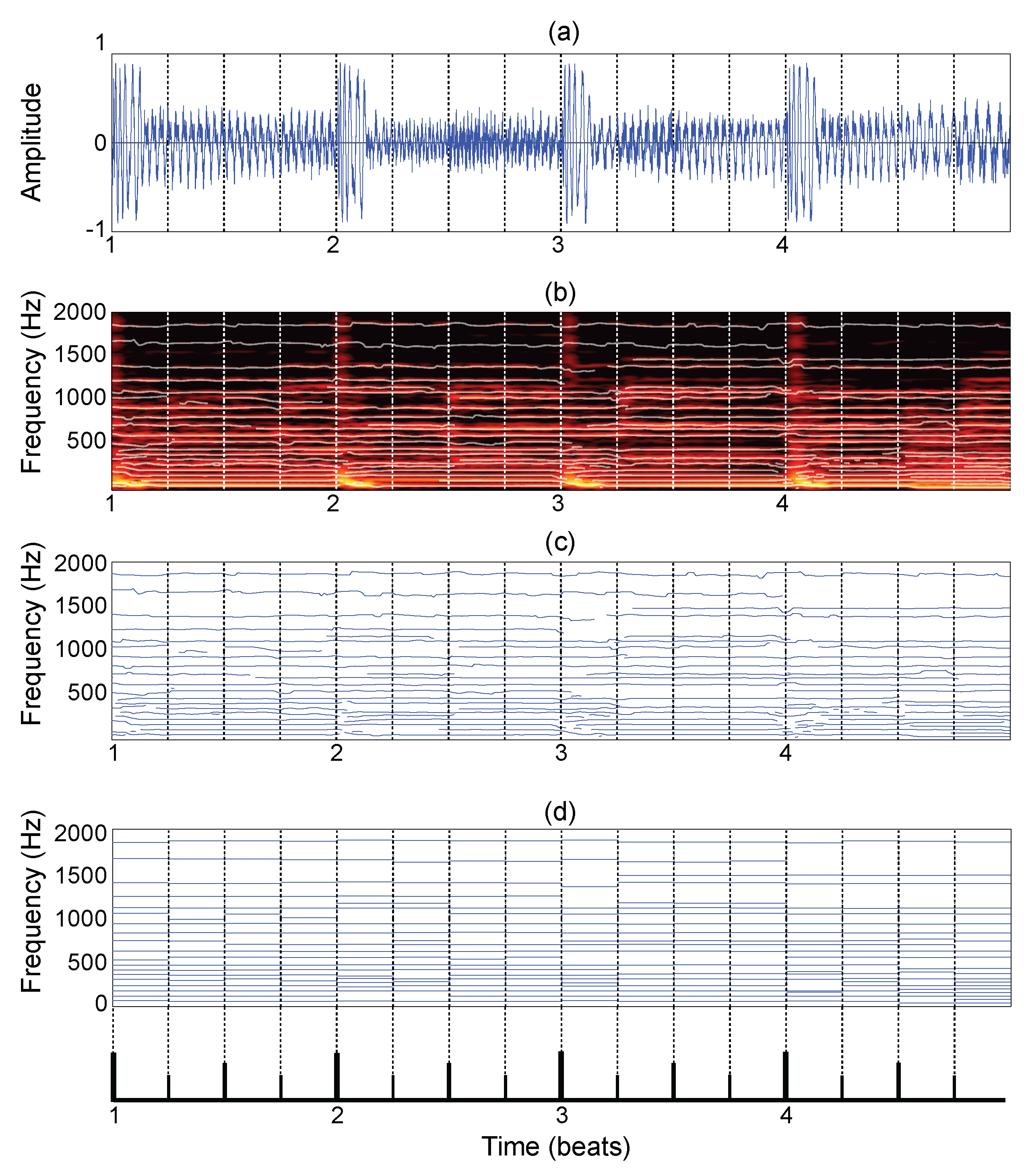
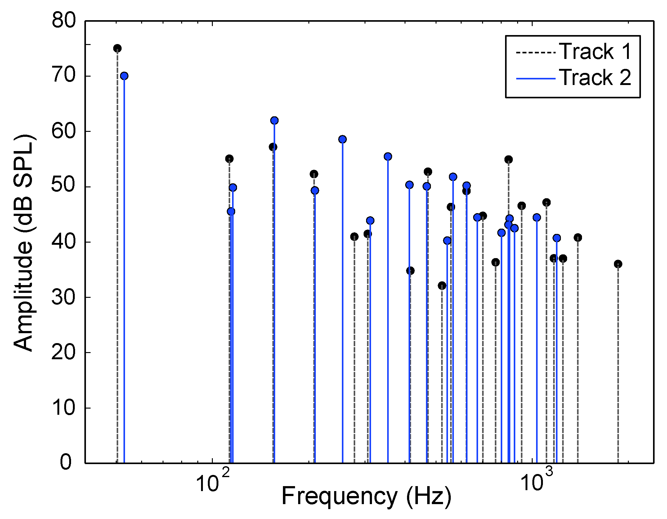
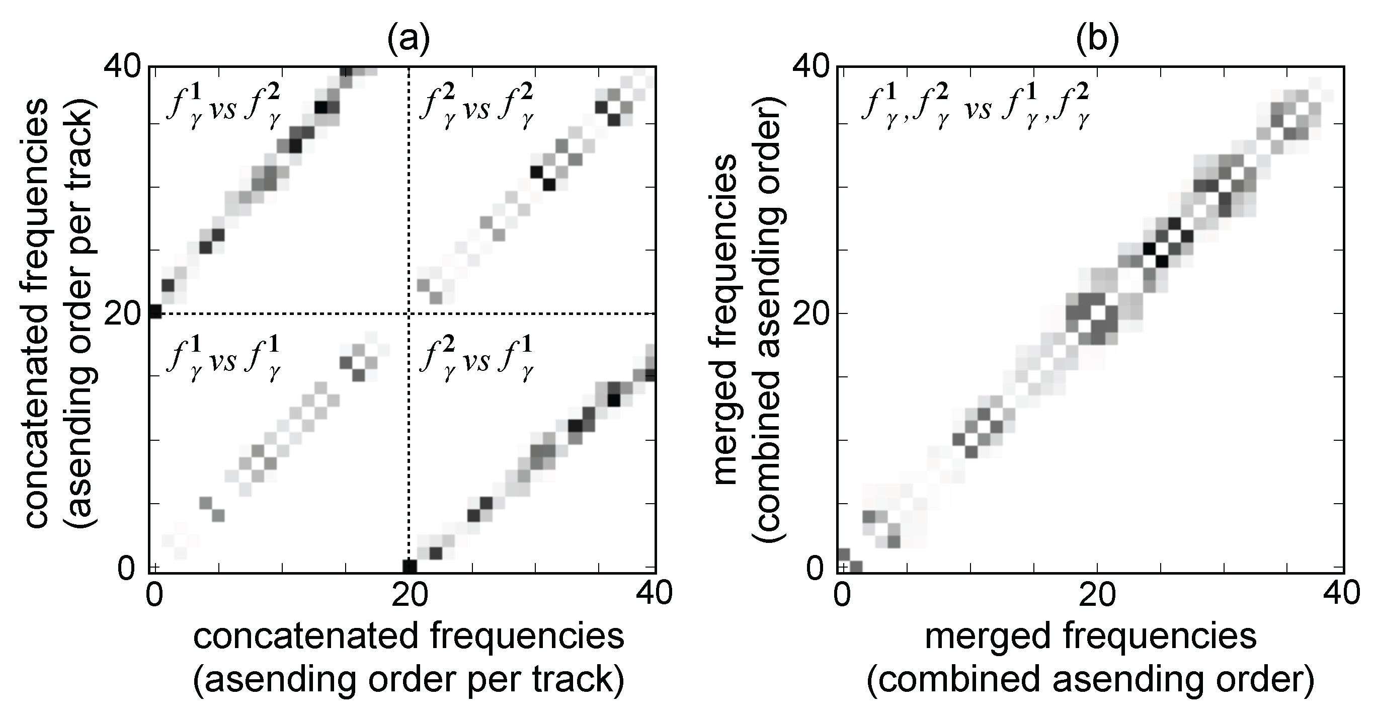
3.1. Data Collection and Pre-Processing

We first explain the necessary pre-processing steps that allow the subsequent measurement of consonance between two pieces of music. For the purpose of this paper, we make several simplifications concerning the properties of the musical audio content we intend to mix.

Given that one of our aims is to compare consonance-based mixing to key-based matching methods in DJ-mixing software (see Section 4), we currently only consider electronic music (e.g., house music), which is both harmonically stable and typically has a fixed tempo. We collected a set of 30 tracks of recent electronic music for which we manually annotated the tempo and beat locations and isolated short regions within each track lasting precisely 16 beats (i.e., four complete bars). In order to focus entirely on the issue of harmonic alignment without the need to address temporal alignment, we force the tempo of each excerpt to be exactly 120 beats per minute. For this beat quantization process, we use the open source pitch-shifting and time-stretching library, Rubber Band [24], to implement any necessary tempo changes. Accordingly, our database of musical excerpts consists of a set of 8 s (i.e., 500 ms per beat) mono .wav files sampled at 44.1 kHz with 16-bit resolution. Further details concerning this dataset are in Section 4.1.

To provide an initial set of frequencies and amplitudes, we use a sinusoidal model, namely the “Spectral Modeling Synthesis Tools” Python software package by Serra [25,26], with which we extract sinusoids using the default window size and hop sizes of 4001 and 256 samples, respectively. In order to focus on the harmonic structure present in the musical input, we extract the $I=20$ partials with the highest amplitude under 5 kHz.

For our chosen genre of electronic music and our assembled dataset, we observed that the harmonic structure remained largely constant over the duration of each 1/16th note (i.e., 125 ms). Therefore, to strike a balance between temporal resolution and computational complexity, we summarize the frequencies and amplitudes by taking the frame-wise median over the duration of each 1/16th note. Thus, for each excerpt, we obtain a set of frequencies and amplitudes, $f_{\gamma ,i}$ and $M_{\gamma ,i}$, where i indicates the partial number (up to $I=20$) and γ each 1/16th note frame (up to $\mathsf{\Gamma }=64$). An overview of the extraction of sinusoids and temporal averaging is shown in Figure 4. In Section 4.2, we examine the effect of this choice of parameters.

3.2. Consonance-Based Alignment

For two input musical excerpts, $T^{\mathbf{1}}$ and $T^{\mathbf{2}}$, with corresponding frequencies and amplitudes $f_{\gamma ,i}^{\mathbf{1}}$,$M_{\gamma ,i}^{\mathbf{1}}$ and $f_{\gamma ,i}^{\mathbf{2}}$,$M_{\gamma ,i}^{\mathbf{2}}$, respectively, we seek to find the optimal consonance-based alignment between them. At this stage, we could attempt to modify (i.e., pitch shift) both excerpts, $T^{\mathbf{1}}$ and $T^{\mathbf{2}}$, so as to minimize the overall stretch factor between them. However, we conceptualize the harmonic mixing problem as one in which there is a user-selected query, $T^{\mathbf{1}}$, to which we will mix $T^{\mathbf{2}}$. In this sense, we can retain the possibility to rank multiple different excerpts in terms of how well they match $T^{\mathbf{1}}$. To this end, we fix all information regarding $T^{\mathbf{1}}$ and modify only $T^{\mathbf{2}}$. This setup offers the additional advantage that only one excerpt will contain artifacts resulting from pitch shifting.

Our approach centers on the calculation of consonance as a function of a frequency shift, s, and is based on the hypothesis that under some frequency shift applied to $T^{\mathbf{2}}$, the consonance between $T^{\mathbf{1}}$ and $T^{\mathbf{2}}$ will be maximized, and this, in turn, will lead to the optimal mix between the two excerpts.

In total, we create $S=97$ shifts, which cover the range of ±6 semitones in 1/8th semitone steps (i.e., 48 downward and 48 upward shifts around a single “no shift” option). We scale the frequencies of the partials $f_{\gamma ,i}^{\mathbf{2}}$ as follows:

$$\begin{array}{cc}{f}_{\gamma ,i}^{\mathbf{2}}[s]=2^{{log}_2(f_{\gamma ,i}^{\mathbf{2}})+\frac{s-48}{96}}\hfill & \hfill s=0,\dots ,S-1.\end{array}$$

(21)

For each 1/16th note temporal frame, γ, and per shift, s, we then merge the corresponding frequencies and amplitudes between both tracks (as shown in Figure 5 and Figure 6), such that:

$$f_{\gamma }[s]=\left[f_{\gamma }^{\mathbf{1}}{f}_{\gamma }^{\mathbf{2}}[s]\right]$$

(22)

and:

$$M_{\gamma }[s]=\left[M_{\gamma }^{\mathbf{1}}{M}_{\gamma }^{\mathbf{2}}[s]\right].$$

(23)

We then calculate the roughness, $D_{\gamma }[s]$ according to Equation (5) in Section 2.1 with the merged partials and amplitudes as input. Figure 7 illustrates the interaction between the partials for a single frame within two equivalent visualizations, first with the partials between the two tracks separated and, then, once they have been merged. In this way, we can observe the interactions between roughness-creating partials between the two tracks in a given frame or, alternatively, examine a visualization that corresponds to their mixture.

Then, to calculate the overall roughness, $\overline{D}[s]$, as a function of frequency shift, s, we take the mean of the roughness values $D_{\gamma }[s]$ across the $\mathsf{\Gamma }=64$ temporal frames of the excerpt:

$$\overline{D}[s]=\frac{1}{\mathsf{\Gamma }}\sum _{\gamma =0}^{\mathsf{\Gamma }-1}{D}_{\gamma }[s],$$

(24)

for which a graphical example is shown in Figure 8.

Having calculated the roughness across all possible frequency shifts, we now turn our focus towards the measurement of pitch commonality as described in Section 2.2. Due both to the high computational demands of the pitch commonality model and the rounding that occurs due to the allocation of discrete pitch categories, we do not calculate the harmonic consonance as a function of all possible frequency shifts. Instead, we extract all local minima from $\overline{D}[s]$, label these frequency shifts, $s^{*}$, and then proceed with this subset. In this way, we use the harmonic consonance, C, as a means to filter and further rank the set of possible alignments (i.e., minima) arising from the roughness model.

While the calculation of $D_{\gamma }[s]$ relies on the merged set of frequencies and amplitudes from Equations (22) and (23), the harmonic consonance compares two individually-calculated Hofman-Engl pitch sets. To this end, we calculate Equations (8) to (17) independently for $f_{\gamma }^{\mathbf{1}}$ and $f_{\gamma }^{\mathbf{2}}[s^{*}]$ to create ${\mathrm{set}}_{\gamma }^{\mathbf{1}}$ and ${\mathrm{set}}_{\gamma }^{\mathbf{2}}[s^{*}]$ and, hence, $C_{\gamma }[s^{*}]$ from Equation (20). As with the roughness, the overall harmonic consonance $\overline{C}[s^{*}]$ is then calculated by taking the mean across the temporal frames:

$$\overline{C}[s^{*}]=\frac{1}{\mathsf{\Gamma }}\sum _{\gamma =0}^{\mathsf{\Gamma }-1}{C}_{\gamma }[s^{*}].$$

(25)

Since no prior method exists for combining the roughness and harmonic consonance, we adopt a simple approach to equally weight their contributions to give an overall measure of consonance based on roughness and pitch commonality:

$$\rho [s^{*}]=\widehat{D}[s^{*}]+\widehat{C}[s^{*}]$$

(26)

where $\widehat{D}[s^{*}]$ corresponds to the raw roughness values $\overline{D}[s^{*}]$, which have been inverted (to reflect sensory consonance as opposed to roughness) and then normalized to the range [0,1], and $\widehat{C}[s^{*}]$ similarly represents the [0,1] normalized version of $\overline{C}[s^{*}]$. The overall consonance $\rho [s^{*}]$ takes values that range from zero (minimum consonance) to two (maximum consonance), as shown in Figure 9. The maximum score of two is achieved only when the roughness and harmonic consonance detect the same pitch shift index as most consonant.

3.3. Post-Processing

The final stage of the consonance-based mixing is to implement the mix between tracks $T^{\mathbf{1}}$ and $T^{\mathbf{2}}$ under the consonance-maximizing pitch shift, i.e., $arg{max}_{s^{*}}(\rho [s^{*}])$. As in Section 3.1, we again use the Rubber Band Library [24] to perform the pitch shifting on $T^{\mathbf{2}}$, as this was found to give better audio quality than implementing the pitch shift directly using the output of the sinusoidal model. To avoid loudness differences between the two tracks prior to mixing, we normalize each audio excerpt to a reference loudness level (pink noise at 83 dB SPL) using the replay gain method [27].

4. Evaluation

The primary purpose of our evaluation is to determine whether the roughness curve can provide a robust means for identifying consonant harmonic alignments between two musical excerpts. If this is the case, then pitch shifting and mixing according to the minima of the roughness curve should lead to consonant (and hence, pleasant) musical results, where as mixing according to the maxima should yield dissonant musical combinations. To explore the relationship between roughness and consonance, we designed and conducted a listening test to obtain consonance and pleasantness ratings for a set of musical excerpts mixed according to different pitch shifts. Following this, we then investigated the effect of varying the main parameters of the pre-processing stage (i.e., the number of partials I and the number of temporal frames Γ), as described in Section 3.1, by examining the correlation between roughness values and listener ratings under different parameterizations.

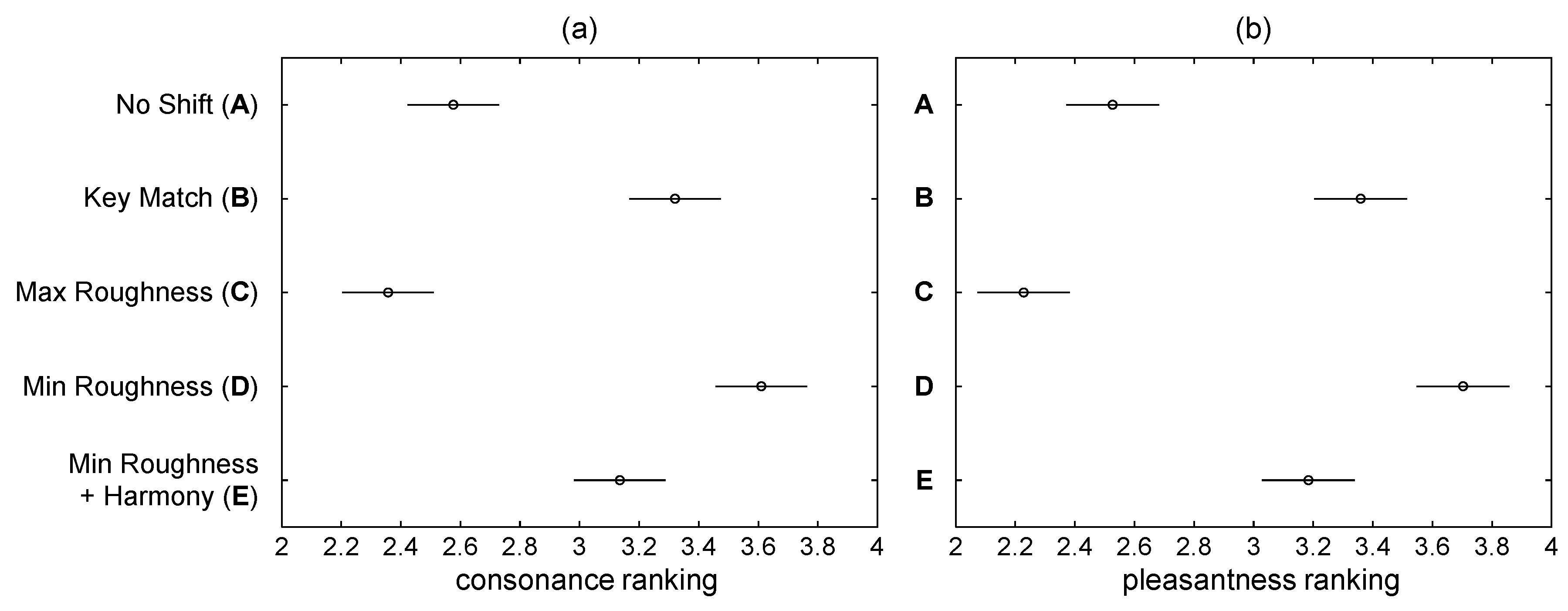
4.1. Listening Test

To evaluate the ability of our model to provide consonant mixes between different pieces of music, we conducted a listening test using excerpts from our dataset of 30 short musical excerpts of recent house music (each 8 s in duration and lasting exactly 16 beats). While our main concern is in evaluating the properties of the roughness curve, we also included a comparison against a key-based matching method using the key estimation from the well-known DJ software Traktor 2 (version 6.1) from Native Instruments [28]. In total, we created five conditions for the mix of two individual excerpts, which are summarized as follows:

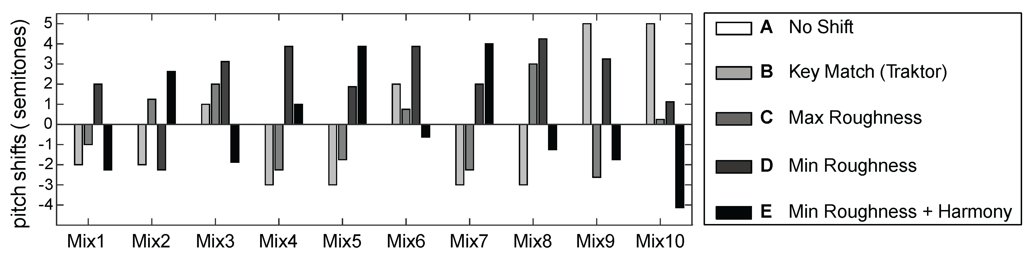
• A No shift: no attempt to harmonically align the excerpts; instead, the excerpts were only aligned in time by beat-matching.
• B Key match (Traktor): each excerpt was analyzed by Traktor 2 and the automatically-detected key recorded. The key-based mix was created by finding the smallest pitch shift necessary to create a harmonically-compatible mix according to the circle of fifths, as per the description in the Introduction.
• C Max roughness: the roughness curve was analyzed for local maxima, and the pitch shift with the highest roughness (i.e., most dissonant) was chosen to mix the excerpts.
• D Min roughness: the roughness curve was analyzed for local minima, and the pitch shift with the lowest roughness (i.e., most consonant) was chosen to mix the excerpts.
• E Min roughness and harmony: from the set of extracted minima in Condition D, the combined harmonic consonance and roughness was calculated, and the pitch shift yielding the maximum overall consonance $\rho [s^{*}]$ was selected to mix the excerpts.

We selected the set of stimuli for use in the listening experiment according to two conditions. First and foremost, we required a set of unique pitch shifts across the five conditions per mix, and second, we chose not to have any repeated excerpts either as input nor the track to be pitch-shifted. To this end, we calculated the pitch shifts for each of the five conditions for all possible combinations of the 30 excerpts in the dataset (introduced in Section 3.1) compared to one other. In total, this provided 900 possible combinations of tracks (including the trivial comparison of each excerpt with itself). A breakdown of the number of matching shifts among the conditions is shown in

Table 1. Number of identical shifts (from a maximum of 900) across each of the conditions resulting from the exhaustive combination of all pairs within the 30 excerpt dataset.

Condition	A	B	C	D	E
A	x	92	7	56	45
B		x	2	100	81
C			x	0	0
D				x	385
E					x

. By definition, there were no matching pitch shifts between Conditions C (max roughness) and D (min roughness) or E (min roughness and harmony). By contrast, Conditions D and E matched 385 times.

Out of 900, a total of 409 combinations gave unique pitch shifts across all five conditions. From this subset of 409, we discarded all cases where the smallest pitch shift between any pair of combinations was lower than 0.25 semitones. Next, we removed all mixes containing duplicate excerpts to avoid single tracks in more than one mix. From this final subset, we kept the 10 mixes (listed in

Table 2. Track titles and artists for the stimuli used in the listening test along with ground truth annotations made by a musical expert. Those excerpts labeled ‘a’ were the inputs to the mixes, whereas those labeled ‘b’ were subject to pitch shifting. In some cases, the harmonic information was too sparse (i.e., too few notes) to make an unambiguous decision between major and minor. In these cases, the predominant root note is indicated. Note, the artist ##### (Mix 4a) is an alias of Aroy Dee (Mix 3b).

Mix No.	Artist	Track Title	Annotated Key
1a	Person Of Interest	Plotting With A Double Deuce	(E)
1b	Locked Groove	Dream Within A Dream	A maj
2a	Stephen Lopkin	The Haggis Trap	(A)
2b	KWC 92	Night Drive	D# min
3a	Legowelt	Elementz Of Houz Music (Actress Mix 1)	B min
3b	Aroy Dee	Blossom	D# min
4a	#####	#####.1	A min
4b	Barnt	Under His Own Name But Also Sir	C min
5a	Julius Steinhoff	The Cloud Song	D min
5b	Donato Dozzy & Tin Man	Test 7	F min
6a	R-A-G	Black Rain (Analogue Mix)	(E)
6b	Lauer	Highdimes	(F)
7a	Massimiliano Pagliari	JP4-808-P5-106-DEP5	(C)
7b	Levon Vincent	The Beginning	D# min
8a	Roman Flügel	Wilkie	C min
8b	Liit	Islando	D# min
9a	Tin Man	No New Violence	C min
9b	Luke Hess	Break Through	A min
10a	Anton Pieete	Waiting	A min
10b	Voiski	Wax Fashion	(E)

) with the lowest maximum pitch shift across the conditions. In total, this provided 50 stimuli (10 mixes × 5 conditions) to be rated. A graphical overview of the pitch shifts per condition is shown in Figure 10, for which sound examples are available in the Supplementary Material. All of the stimuli were rendered as mono .wav files at a sampling rate of 44.1 kHz and with 16-bit resolution.

In total, 34 normal hearing listeners (according to a self-report) participated in the experiments. Their musical training was self-rated as being either: music students, practicing musicians or active in DJing. Eleven of the participants were female, and 23 were male; their ages ranged between 23 and 57. When listening to each mix, the participants were asked to rate two properties: first, how consonant and, second, how pleasant the mixes sounded to them. The question for pleasantness was introduced both to emphasize the distinction between personal taste and musical consonance to the listener and also to consider the fact that a higher level of consonance might not lead to a more pleasant listening experience [9]. Both conditions were rated on a discrete six-point scale (zero to five) using a custom patch developed in Max/MSP. The order of the 50 stimuli was randomized for each participant. After every sound example, the ratings had to be entered before proceeding to the next. To guarantee familiarity with the experimental procedure and stimuli, a training phase preceded the main experiment. This was also used to ensure all participants understood the concept of consonance and to set the playback volume to a comfortable level. All participants took the experiment in a quiet listening environment using high quality headphones.

Regarding our hypotheses on the proposed conditions, we expected Condition C (max roughness) to be the least consonant, followed by A (no shift). However, without any harmonic alignment, its behavior was not easily predictable, save for the fact that it would be at least 0.25 semitones from any other condition. Of the remaining conditions, which attempted to find a good harmonic alignment, we expected B (Traktor) to be less consonant than both D (min roughness) and E (min roughness and harmony).

4.2. Results

4.2.1. Statistical Analysis

To examine the data collected in the listening experiment, we separately analyzed the consonance and pleasantness ratings using the non-parametric Friedman test where we treated participants and mixes as random effects. For both the consonance and pleasantness ratings, the main effect of the conditions was highly significant (consonance: chi-square = 181.60, p < 0.00001; pleasantness: chi-square = 240.73, p < 0.00001).

With regard to the interaction across conditions, we performed a post hoc analysis via a multiple comparison of means with Bonferroni correction for which the mean rankings and 95% confidence intervals are shown in Figure 11a,b for consonance and pleasantness ratings, respectively.

There is a very large separation between Conditions B, D and E, i.e., those conditions that attempt to find a good harmonic alignment, and Conditions A and C, which do not. No significant difference was found between Conditions A and C (consonance: p > 0.45; pleasantness: p > 0.07) and likewise for conditions B and E (consonance: p > 0.90; pleasantness: p = 1.00). For consonance, the difference between Conditions D and B is not significant, p > 0.08; however it is significant for pleasantness p < 0.05.

Inspection of Figure 11 reveals similar patterns regarding consonance and pleasantness ratings, which are generally consistent with our hypotheses stated in Section 4.1. Ratings for Condition C (max roughness) are significantly smaller (worse) than for all other conditions, except Condition A (no shift). Pitch shifts in Condition D (min roughness) are rated significantly highest (best) in terms of pleasantness ratings.

While there is a large separation between the ratings for Conditions D and E, i.e., our two proposed methods for consonance, such a result should be examined within the context of the experimental design and additional inspection of Table 1. Here, we find that close to 43% of the 900 combinations resulted in an identical choice of pitch shift, implying that both methods often converged on the same result and to a far greater degree than any of the other condition pairs. Since there is no significant difference between the ratings of Conditions E and B and because these were rated towards the higher end of the (zero to five) scale, we could consider any of three methods to be a valid means of harmonically mixing music signals, nevertheless with Condition D the preferred choice.

Looking again at the key-based approach (Condition B), it is useful to consider the impact of any misestimation of the key made by Traktor. To this end, we asked a musical expert to annotate the ground truth keys for each of the 20 excerpts used to make the listening test. These annotated keys are shown in Table 2. Despite the apparent simplicity of this type of music from a harmonic perspective, our music expert was unable to precisely label the key in six out of the 20 cases. This was due to the short duration of the excerpts and an insufficient number of different notes to unambiguously choose between a major or minor key. In these cases, the most predominant pitch class was annotated instead. Traktor, on the other hand, always selects a major or minor key (irrespective of the tonality of the music), and in fact, it only agreed with our expert in six of the cases. In addition, we used Traktor to extract the key for the full-length recordings, and in these cases, the key matched between the excerpt and full-length recording only eight out of 20 times. While the inability of Traktor to extract the correct key should lead us to expect poor performance in creating harmonic mixes, this is not especially evident in the results. In fact, it may be that the harmonic simplicity (i.e., the weak sense of any one predominant key) in the excerpts of our chosen dataset naturally lends itself to multiple different harmonic alignments; an observation supported by the results, which show more than one possible option for harmonic alignment being rated towards the higher end of the scales for consonance and pleasantness. A graphical example comparing the output of the key-based matching using Traktor (Condition B) and min roughness (Condition D) between two excerpts is shown in Figure 12.

4.2.2. Effect of Parameterization

Having looked into detail at the interactions between the difference conditions in terms of the ratings, we now revisit the properties of the roughness curve towards understanding the extent to which it provides a meaningful indicator of consonance for harmonic mixing.

To this end, we now investigate the correlation between the ratings obtained from consonance and pleasantness compared to the corresponding points in the roughness curve for each associated pitch shift. While only three of the five conditions (C, D and E) were derived directly from each roughness curve, for completeness, we use the full set of 50 points (i.e., five conditions across 10 mixes).

To gain a deeper insight into the design of our model, which is highly dependent on the extraction of partials using a sinusoidal model, we generate multiple roughness curves under different parameterizations and measure the correlation with the listener ratings for each. We focus on what we consider to be the two most important parameters: I, the number of sinusoids, and Γ, the number of temporal frames after averaging. In this way, we can examine the relationship from a harmonic and temporal perspective. To span the parameter space, we vary I from five up to 80 (default value = 20), and for the temporal averaging, we consider three cases: (i) beat level averaging (Γ = 16 across four-bar excerpts); (ii) 16th note averaging (Γ = 64 and our default condition); and (iii) using all frames from the sinusoidal model without any averaging. The corresponding plots for both consonance and pleasantness ratings are shown in Figure 13.

From inspection of the figure, we can immediately see that the number of sinusoids plays a more critical role than the extent/use of temporal averaging. Using more than 25 sinusoids (per frame of each track) has an increasingly negative impact on the Pearson correlation value. Likewise, using too few sinusoids also appears to have a negative impact. Considering the roughness model, having too few observations of the harmonic structure will very likely fail to capture all of the main roughness creating partials. While on the other hand, over-populating the roughness model with sinusoids (many of which may result from percussive or noise-like content) will also obscure the interaction of the “true” harmonic partials in each track. Within the context of our (harmonically simple) dataset, a range of between 15 and 25 partials provides the strongest relationship between roughness values and consonance ratings.

Looking next at the effect of the temporal averaging, we can see a much noisier relationship when using beat averaging compared to our chosen summarization at the 16th note level. In contrast, the plot is smoothest without any temporal averaging, yet it is moderately less correlated with the data. As with the harmonic dimension, the 16th note segmentation adequately captures the rate at which harmonic content changes in the signal, without losing too much fine detail through the temporal averaging process.

Finally, comparing the plots side by side, we see a near identical pattern for consonance and pleasantness. This behavior is to be expected given the very high correlation between the consonance and pleasantness ratings themselves (r = 0.76, p < 1×10${}^{-}$${}^6$). In the context of our dataset, this implies that the participants of the listening test considered consonance and pleasantness to be highly inter-dependent and, thus, that the measurement of roughness is a reliable indicator of listener preference for harmonic mixing.

5. Conclusions

In this paper, we have presented a new method for harmonic mixing ultimately targeted towards addressing some of the limitations of key-based DJ-mixing systems. Our approach centers on the use of psychoacoustic models of roughness and pitch commonality to identify an optimal harmonic alignment between different pieces of music across a wide range of possible fine-scaled pitch shifts applied to one of them. Via a listening experiment with musically-trained participants, we demonstrated that, within the context of the musical stimuli used, mixes based on a minimum degree of roughness were perceived as significantly more pleasant than those aligned according to musical key. Furthermore, including a harmonic consonance model in addition to the roughness model provided alternative pitch shifts, which were rated as consonant and pleasant as those from a commercial DJ-mixing system.

Concerning areas for future work, our model has thus far only been tested on very short and harmonically-simple musical excerpts, and therefore, we intend to test it under a wider variety of musical stimuli, including excerpts with more harmonic complexity. In addition, we plan to focus on the adaptation of our model towards longer musical excerpts, perhaps through the use of some structural segmentation into harmonically-stable regions.

We have also yet to consider the role of music with vocals and how to examine the potentially unnatural results that arise from pitch shift singing. To this end, we will explore both singing voice detection and voice suppression. Along similar lines, our roughness-based model can reveal not only which temporal frames give rise to the most roughness, but also precisely which partials contribute within these frames. Hence, we plan to explore methods for the suppression of dissonant partials, towards more consonant mixes.

Lastly, in relation to the interaction between the harmonic consonance and roughness, we will reexamine the rather simplistic combination of these two sources of information, towards a more sophisticated two-dimensional model of sensory roughness and harmony.

References

- Ishizaki, H.; Hoashi, K.; Takishima, Y. Full-automatic DJ mixing with optimal tempo adjustment based on measurement function of user discomfort. In Proceedings of the International Society for Music Information Retrieval Conference, Kobe, Japan, 26–30 October 2009; pp. 135–140.
- Sha’ath, I. Estimation of Key in Digital Music Recordings. Master’s Thesis, Birkbeck College, University of London, London, UK, 2011. [Google Scholar]
- Davies, M.E.P.; Hamel, P.; Yoshii, K.; Goto, M. AutoMashUpper: Automatic creation of multi-song mashups. IEEE/ACM Trans. Audio Speech Lang. Process. 2014, 22, 1726–1737. [Google Scholar] [CrossRef]
- Lee, C.L.; Lin, Y.T.; Yao, Z.R.; Li, F.Y.; Wu, J.L. Automatic Mashup Creation By Considering Both Vertical and Horizontal Mashabilities. In Proceedings of the International Society for Music Information Retrieval Conference, Malaga, Spain, 26–30 October 2015; pp. 399–405.
- Terhardt, E. The concept of musical consonance: A link between music and psychoacoustics. Music Percept. 1984, 1, 276–295. [Google Scholar] [CrossRef]
- Terhardt, E. Akustische Kommunikation (Acoustic Communication); Springer: Berlin, Germany, 1998. (In German) [Google Scholar]
- Gebhardt, R.; Davies, M.E.P.; Seeber, B. Harmonic Mixing Based on Roughness and Pitch Commonality. In Proceedings of the 18th International Conference on Digital Audio Effects (DAFx-15), Trondheim, Norway, 30 November–3 December 2015; pp. 185–192.
- Hutchinson, W.; Knopoff, L. The significance of the acoustic component of consonance of Western triads. J. Musicol. Res. 1979, 3, 5–22. [Google Scholar] [CrossRef]
- Parncutt, R. Harmony: A Psychoacoustical Approach; Springer: Berlin, Germany, 1989. [Google Scholar]
- Hofman-Engl, L. Virtual Pitch and Pitch Salience in Contemporary Composing. In Proceedings of the VI Brazilian Symposium on Computer Music, Rio de Janeiro, Brazil, 19–22 July 1999.
- Parncutt, R.; Strasburger, H. Applying psychoacoustics in composition: “Harmonic” progressions of “non-harmonic” sonorities. Perspect. New Music 1994, 32, 1–42. [Google Scholar] [CrossRef]
- Hutchinson, W.; Knopoff, L. The acoustic component of western consonance. Interface 1978, 7, 1–29. [Google Scholar] [CrossRef]
- Plomp, R.; Levelt, W.J.M. Tonal consonance and critical bandwidth. J. Acoust. Soc. Am. 1965, 38, 548–560. [Google Scholar] [CrossRef] [PubMed]
- Sethares, W. Tuning, Tibre, Spectrum, Scale, 2nd ed.; Springer: London, UK, 2004. [Google Scholar]
- Bañuelos, D. Beyond the Spectrum of Music: An Exploration through Spectral Analysis of SoundColor in the Alban Berg Violin Concerto; VDM: Saarbrücken, Germany, 2008. [Google Scholar]
- Parncutt, R. Parncutt’s Implementation of Hutchinson & Knopoff. 1978. Available online: http://uni-graz.at/parncutt/rough1doc.html (accessed on 28 January 2016).
- Moore, B.; Glassberg, B. Suggested formulae for calculating auditory-filter bandwidths and excitation patterns. J. Acoust. Soc. Am. 1983, 74, 750–753. [Google Scholar] [CrossRef] [PubMed]
- MacCallum, J.; Einbond, A. Real-Time Analysis of Sensory Dissonance. In Computer Music Modeling and Retrieval. Sense of Sounds; Kronland-Martinet, R., Ystad, S., Jensen, K., Eds.; Springer: Berlin, Germany, 2008; Volume 4969, pp. 203–211. [Google Scholar]
- Vassilakis, P.N. SRA: A Web-based Research Tool for Spectral and Roughness Analysis of Sound Signals. In Proceedings of the Sound and Music Computing Conference, Lefkada, Greece, 11–13 July 2007; pp. 319–325.
- Terhardt, E.; Seewan, M.; Stoll, G. Algorithm for Extraction of Pitch and Pitch Salience from Complex Tonal Signals. J. Acoust. Soc. Am. 1982, 71, 671–678. [Google Scholar] [CrossRef]
- Hesse, A. Zur Ausgeprägtheit der Tonhöhe gedrosselter Sinustöne (Pitch Strength of Partially Masked Pure Tones). In Fortschritte der Akustik; DPG-Verlag: Bad-Honnef, Germany, 1985; pp. 535–538. (In German) [Google Scholar]
- Apel, W. The Harvard Dictionary of Music, 2nd ed.; Harvard University Press: Cambridge, UK, 1970. [Google Scholar]
- Hofman-Engl, L. Virtual Pitch and the Classification of Chords in Minor and Major Keys. In Proceedings of the ICMPC10, Sapporo, Japan, 25–29 August 2008.
- Rubber Band Library. Available online: http://breakfastquay.com/rubberband/ (accessed on 19 January 2016).
- Serra, X. SMS-tools. Available online: https://github.com/MTG/sms-tools (accessed on 19 January 2016).
- Serra, X.; Smith, J. Spectral modeling synthesis: A sound analysis/synthesis based on a deterministic plus stochastic decomposition. Comput. Music J. 1990, 14, 12–24. [Google Scholar] [CrossRef]
- Robinson, D. Perceptual Model for Assessment of Coded Audio. Ph.D. Thesis, University of Essex, Colchester, UK, March 2002. [Google Scholar]
- Native Instruments Traktor Pro 2 (version 6.1). Available online: http://www.native-instruments.com/en/products/traktor/dj-software/traktor-pro-2/ (accessed on 28 January 2016).