1. Introduction
World population and energy demand are increasing rapidly. The provision of reliable and sustainable energy services according to 21st century requirements is becoming more challenging day by day [
1,
2,
3]. Real-time monitoring, dynamic control and users’ active participation in energy services are vital to ensure a sustainable future. The traditional grid is not supposed to provide such dynamic services because of its aged infrastructure. It is needed to convert the traditional grid into a smart grid in order to meet the energy management challenges [
4,
5,
6]. The smart grid is envisioned to provide sustainable energy services dynamically and efficiently to fulfill the requirements of meeting the ever increasing demand and addressing the green concerns. Various applications of smart grid are mentioned in literature such as smooth integration of renewable resources, transmission and distribution automation, optimized energy management
etc. [
7,
8].
Demand Side Management (DSM) is one of the important aspects of optimal energy management in which consumers’ behavior is influenced to manage the electricity consumption [
9]. Home Energy Management Systems (HEMS) are found among important smart grid applications to ensure DSM [
10,
11]. HEMS help in peak load reduction and consumers’ total energy cost minimization by using embedded sensors and Advanced Metering Infrastructure (AMI). Consequently, use of peaker plants and carbon footprint are reduced, which are desirable and important for sustainable future [
12].
Although peak load reduction can be achieved in several different ways, appliance scheduling is one of the promising methods for this purpose. A novel energy management mechanism, namely Comprehensive Home Energy Management Architecture (CHEMA), is presented in this paper. CHEMA consists of a six-layer model with multiple scheduling options, and it has been implemented in Simulink with embedded MATLAB code. Important contributions of this work are listed as the following:
A unique HEMS architecture which covers more aspects of the residential energy management problem and multiple cost minimization options integrated at the second layer;
Formulation of optimization problem which is unique with the concept of partial base line load and its inclusion in the optimization problem, discussed in detail in
Section 3;
Control of lighting and heating loads with the help of a Persons Presence Controller (PPC);
Solution of the energy cost optimization problem with a single Knapsack technique with embedded Matlab code in Simulink.
The remaining paper is arranged as follows.
Section 2 presents related work and
Section 3 is dedicated for the proposed architecture. The results are elaborated in
Section 4 and conclusions are drawn in
Section 5.
2. Related Work
Various pricing strategies have been designed for users’ energy cost minimization [
13]. For instance, a day ahead pricing scheme has been used in [
14] for appliance scheduling in order to minimize total energy cost. Authors in [
15] proposed a Linear Programming (LP) model to optimize the home energy consumption and total cost. In this model, a full day is divided into equal length time slots with changing prices just like Time of Use (ToU) tariff.
A Dynamic Demand Response Controller (DDRC) has been designed in [
16]. The purpose of DDRC is to control the Heating Ventilation Air Conditioning (HVAC) unit according to Real-Time Pricing (RTP) signals. The controller considers thermal properties of construction materials in order to calculate the thermal insulation and losses. DDRC switches between cooling and heating modes on the basis of threshold temperature and has been tested on a single family house model. DDRC is limited to the HVAC only, and we have presented a cost minimization model with three load categories and multiple scheduling options.
Authors in [
17] have proposed a distributed DSM model in which users are equipped with energy storage facilities. Game theory has been applied in the proposed model to set the energy consumption and the storage game. Distributed algorithms ensure users’ privacy and cost minimization.
A Model Predictive Control (MPC) framework has been proposed for peak load shaving by optimal use of storage batteries in [
18]. Markov process and an “update” algorithm have been used to predict a user’s location and update the energy matrix accordingly. This model considers the single user location for prediction of energy consumption. Our proposed model, CHEMA, considers a multiple number of users present in different time slots to control lighting load and hot water consumption.
A system architecture has been presented in [
19], which includes three layers. The first layer is the named Admission Controller (AC), and it uses the modified spring algorithm for management of requests of appliances. The second layer is used for optimization of home energy management and is called the Load Balancer (LB). Mix integer programming is used at this layer to generate the optimized schedule for appliances. The third layer is proposed for the smart grid interface and has not been implemented in the scheme. We have proposed a new CHEMA model, which consists of six layers and multiple energy management options for users. CHEMA is based on enhanced load categories, multiple scheduling options and flexible user comfort index with relaxed temperature limits. Unique features of CHEMA include: use of multiple cost minimization options with a single Knapsack technique with inclusion of partial base line load in optimization problem. The same model includes the theft and faults detection capability along with calculations of green effects at residential level. The model also takes account of the number of users present at home to control the partial base line load and hot water consumption. Inclusion of these features make CHEMA a unique comprehensive model. On the basis of the discussion above, we have included the following features in CHEMA.
The proposed system architecture in [
19] has three layers. However, there are certain aspects regarding HEMS, which should be included in the HEMS architecture to make it more comprehensive,
i.e., inclusion of green effects, detection of theft and faults at residential level and incorporation of multiple pricing schemes in order to use it at different occasions.
Generally, three categories of appliances have been used in literature: base line load, regular load and burst load. Base line load consists of essential loads such as fans, lighting, etc. This type of load can be included into schedulable load on partial or half basis.
The definition of thermal comfort zone instead of sharp threshold to switch on/off the thermal loads is also helpful in cost minimization and peak load reduction. Suitable comfort zone definition, and its implementation is also necessary for comprehensive energy management architecture.
Total cost minimization for a single user has been done extensively in literature; however, the effect of the users present at different times effects the load consumption. The effect of the number of the persons present for lighting loads and hot water consumption cause effective reduction in the total cost.
We are proposing a six-layered architecture, CHEMA, which includes the above mentioned features. Energy cost minimization problem with multiple options has been solved at the second layer of CHEMA. Details of CHEMA are elaborated on in the subsequent section.
3. Proposed CHEMA and its Implementation
This section elaborates on the details of CHEMA and its implementation. Household appliances could be characterized on the basis of energy or power consumption. A major portion of the household appliances, almost 63%, consists of energy based loads and is very useful for DSM purposes [
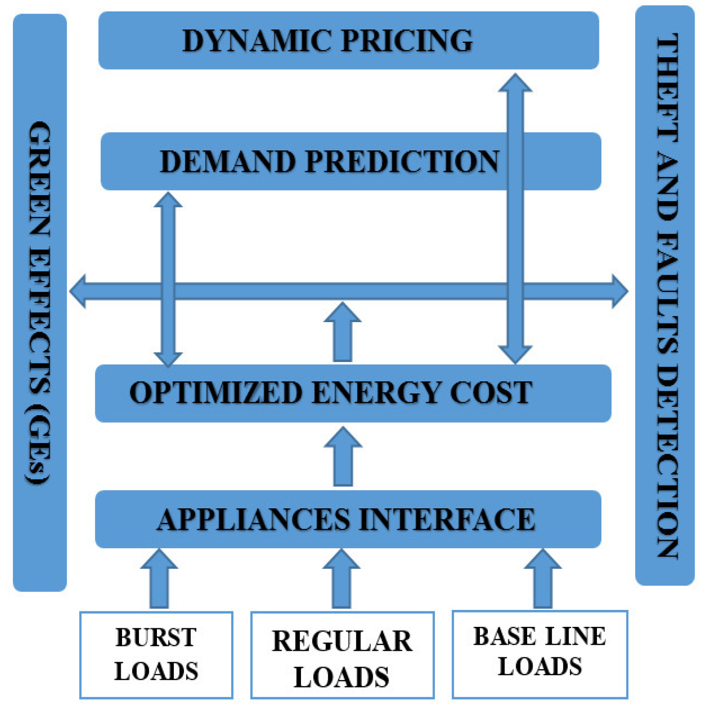
20]. These loads include water heaters, space heaters, air conditioners and refrigerators. We have added these basic loads in CHEMA with least impact on user comfort. Our proposed model consists of six layers: Appliance Interface (AI), Optimized Energy Cost (OEC), Theft and Faults Detection (TFD), Green Effects (GEs), Demand Prediction (DP), and Dynamic Pricing. Basic layout of the proposed CHEMA is depicted in
Figure 1.
The first layer is used for the appliance interface, i.e., basic parameters used for modelling of various appliances and energy cost minimization algorithm are provided using a MATLAB (R2007a, National University of Science and Technology (NUST), Islamabad, Pakistan) file. Appliance rating, required slots, and capacity is loaded through this file. The second layer is used to execute four different cases of the energy cost minimization. The results of the second layer are used to detect the electricity theft and faults at the third layer. Finally, green effects are calculated at the fourth layer, and purpose of this layer is to motivate the users to reduce the energy consumption by displaying carbon emissions at users’ premises.
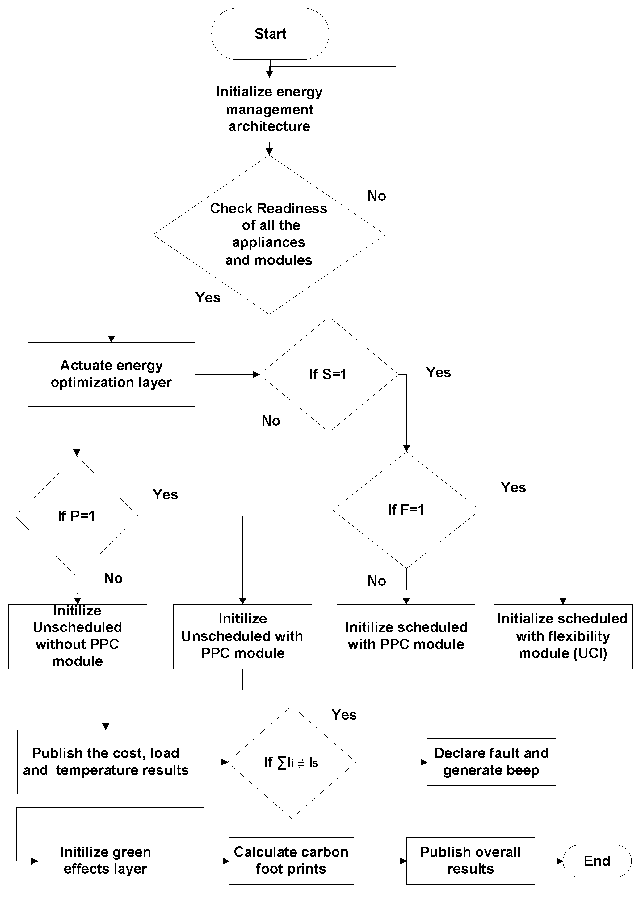
The fifth layer is demand prediction, which is not implemented in our work; however, the purpose of including this layer in CHEMA is to enhance its capability of energy cost minimization in the context of short term load forecasting of users’ load. The sixth layer is proposed for the dynamic pricing information. It is supposed that, in the smart grid environment, users are equipped with an advanced communication and control link with utility through the smart meter in order to get the real-time pricing information. The utility is also capable of monitoring the users’ consumption in real-time by using the same communication link. We have used the ToU pricing scheme in CHEMA; however, the purpose of the dynamic pricing layer is to propose the inclusion of dynamic scheduling ability to CHEMA in the context of real-time information obtained from utility. We have implemented four out of the six layers in this paper. In CHEMA, all the appliances are interfaced with the first layer and basic parameters of all the appliances are loaded into the MATLAB workspace. In the case of missing parameters while loading, the model generates the error message and does not proceed to the next layer. The second layer is dedicated for energy cost optimization. Four energy management and cost minimization cases are implemented at this layer: unscheduled energy cost model, unscheduled with PPC, scheduled with PPC and scheduled with flexibility. The single Knapsack optimization technique is used for scheduling options. The third layer is used for theft and fault detection purposes and is based on a malicious node detection strategy. Whenever faults (e.g., phase to ground fault) occur, the model detects it and a beep is generated for a user’s immediate attention. The fourth layer is used for GEs. The remaining two layers are proposed for demand prediction or load forecasting effects and dynamic pricing, respectively. ToU pricing scheme has been used in this model. However, various dynamic pricing models may be implemented at this layer. Complete flow chart of CHEMA is depicted in
Figure 2.
After the basic parameters’ initialization at AI, the CHEMA algorithm checks for value of
S, which stands for schedulability. If the value of
S is 1, the algorithm goes to scheduling options; otherwise, it goes to unscheduled options. Furthermore, it checks for two parameters:
P and
F, which stand for PPC and flexibility, respectively. If
P = 1, CHEMA activates the unscheduled with PPC energy cost minimization option; otherwise, it is confined to the unscheduled option. If
F is one, the flexibility option is actuated. Whichever option is actuated, the power consumption, temperature variations and total cost results are displayed accordingly. In
Figure 2,
represents the appliances current and
represent the source current. Now, the running or operational appliances are interfaced simultaneously with TFD and GE layers. Faults and theft are detected at the third layer, and the user is informed about abnormal conditions by beep generation. Carbon footprints are calculated in the fourth layer in order to make users more conscious about environmental concerns. Runtime observation of cost and carbon footprints surely affects the users’ energy consumption behavior. Various aspects and modules of CHEMA are explained in subsequent sections.
3.1. Load Categorization
Home appliances are categorized with respect to different aspects in literature [
21]. Generally, there are three major categories of home appliances: essential load or baseline load, regular or continuously running load and burst or schedulable loads. In CHEMA, load has been divided into the following categories and subcategories.
The first category is of essential load which includes: lighting, fans and communication equipment only. Lighting can be divided into sub categories of off-peak lighting in such a way that peak lighting is at least up to half of the off-peak lighting.
where
shows the total lighting load and
denotes off-peak lighting load. This load is partially added in the scheduling problem. Inclusion of essential loads on a half-basis as indicated in Equation (
1), such as lighting load, is the enhancement in the optimization problem presented in [
19]. It will minimize the cost more effectively with the control of the lighting in peak hours. Therefore, base line load is partially added into scheduling problem. In addition, in off-peak hours, the lighting is controlled on the basis of no. of persons present in the house. If the set of time slots is presented by
and
is the total no. of time slots and the set of persons is presented as
, and
shows the maximum no. of persons in the house, then
where,
,
etc. belong to
T. The second major category is of regular or continuous running loads which include: refrigerator, central heating/cooling, water heater
etc. The third major category is of schedulable loads which include: water pump, electric iron, washing machine and dishwasher,
etc. We are introducing flexible load categorization, which is explained with the help of the following scenarios:
HVAC temperatures are given a tolerance band yet maintain reasonable comfort of the user,
Hot water consumption is controlled with PPC, i.e., on the basis of persons present at home.
3.2. Energy Cost Optimization Model
In light of the above discussion, the scheduling problem has been formulated for a set of appliances
in a horizon of 24 equal time slots, which are represented by a set of
. Appliances’ power rating and per unit energy cost are used for calculating the cost for each category of the load. If
,
and
represent the burst, regular and partial baseline loads and
,
and
represent the ON and OFF states of the corresponding category with 1 and 0 values, respectively. The optimization problem will be as follows:
The final objective function can be written as:
subject to:
where
electricity cost in time slot j
capacity of burst load
capacity of regular load
capacity of partial baseline load
j time slot
T total time horizon
appliance ON/OFF status
total electricity cost.
The binary optimization problem described in Equations (4), (4a), and (4b) is solved for different scheduling options using the single Knapsack technique. Implementation of various Simulink modules is described in subsequent sections.
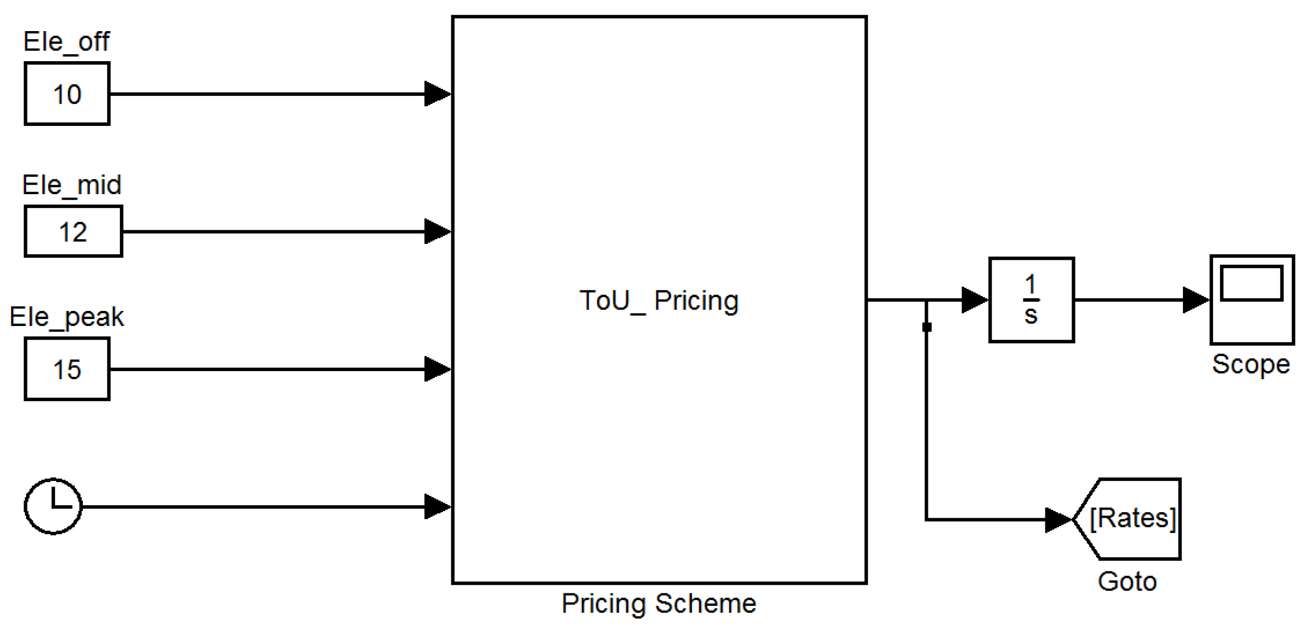
3.3. Pricing Scheme
There are various pricing strategies in dynamic energy management modeling such as ToU, RTP, CPP,
etc. In CHEMA, the ToU pricing scheme is used and rates are taken as Pakistani Rupees (PKR) 10.0/kWh (0.094 USD) for off-peak hours, PKR 12.0/kWh (0.113 USD) for mid peak and PKR 15.0/kWh (0.141 USD) for peak hours. The scheme is implemented in Simulink with clock and embedded code as shown in
Figure 3. Rates of this module are used at various places to compute the energy cost.
3.4. Space Heating Module
The space heating module calculates the heating cost on the basis of the modelled environment, thermal parameters of premises and the heating system. Initial room temperature is taken as 20
C or 68
F. The model is based on the following differential equations [
22,
23]:
where
represents the flow of heat from heater into the room,
is heater temperature,
is room temperature,
is the mass of air, and
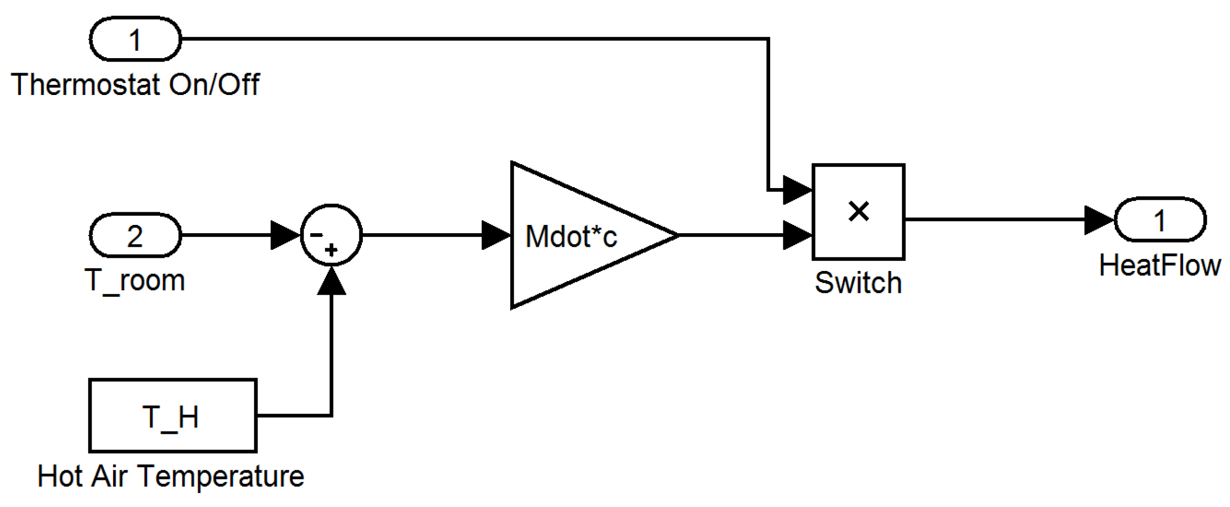
c is the specific heat capacity of the air. Room temperature variations are calculated on the basis of net heat flow by considering the heat losses as elaborated in the following equations:
where
represents the equivalent thermal resistance of the room. “Thermostat” block is used to switch ON and OFF the heater with 5
F variations. The heater subsystem is shown in the
Figure 4.
3.5. Water Heater and Refrigerator Modules
The water heater is another important load with thermal storage capability used in CHEMA for energy management. Water heaters are considered the second largest load among household appliances and consume about 30% of the total energy consumed [
24]. Electrical energy supplied to water heaters is divided into two parts: one is used for heating of cold water and the other is consumed for compensation of heat losses from tank to ambient. There are two ways for heat loss in water heaters: one is conduction losses through walls of the heater and the other is temperature drop by water drawn for usage and entry of colder water for compensation. Energy flow analysis of the water heater provides the following differential equation to determine the inside temperature of water. On the basis of heat flow, the water heater model is given by the following equation [
24]:
where
τ: initial time (h)
: initial temperature (F)
: incoming water temperature (F)
: ambient air temperature outside tank (F)
: temperature of water in tank at time t (F)
Q : energy input rate as function of time (W)
R : tank thermal resistance (mF/W)
SA : surface area of tank (m
G = SA/R (W/ F)
: water demand (L/h)
: specific heat of water (W/Fkg)
D : density of water = 1 kg/L
B : D.. (W/ F)
C : (volume of tank)(density of water) (W/ F)
(W/F).
Water temperature inside the heater is represented on left hand, ambient losses, energy required for water heating and total input are taken on the right hand side of the equation. Refrigerator modeling is based on Equation (9) as follows:
where
,
and
represent the outdoor temperature, the room temperature and wall temperature, respectively. This equation gives the approximate temperature of the refrigerator wall.
The refrigerator system consists of three subsystems. The first and second subsystems are used to implement the wall and indoor temperatures, respectively. The third subsystem compares the indoor temperature and set point to turn ON/OFF the refrigerator. The same module is used to convert the joules into watts and perform subsequent cost calculations according to given rates.
3.6. TFD
Electricity theft and fault identification are important user concerns which are also addressed in CHEMA. There are many ways for theft detection and minimization [
25,
26]. One simple approach is that whenever a line to ground fault occurs or some theft attempt is made, there is a change of total current of house loads. This fact is used in the development of faults and theft identification module. If
is the total current required by all the on appliances and
,
, .....
represent the “
n” appliance current then,
where
represents the
appliance current and
shows the source current. Fault is detected in real-time and a beep is generated for users’ immediate attention.
3.7. GEs
Another layer of environmental concerns or green effects has been introduced in order to relate the residential energy consumption to the Green House Gases (GHGs) emission or carbon footprint. Carbon footprints are defined as “the total sets of GHG emission caused by an organization, event, product or person” [
27]. GHGs in the earth’s atmosphere are water vapor, carbon dioxide, methane, nitrous oxide and ozone. These gases absorb and emit radiations within thermal infrared range and cause the GEs.
In order to make the calculations simple, Wright, Kemp, and Williams have suggested the definition as: “the measure of total amount of CO
and Methane (CH
) emission of a defined population, system or activity, considering all relevant sources, sinks storage within the spatial and temporal boundaries of population, system or activity of interest” [
27].
The reduction of carbon footprints by developing alternative projects such as solar and wind energy is called carbon offsetting [
28]. GHGs can be measured by monitoring the emissions continuously or by estimating the data related to emissions,
i.e., (amount of fuel) and applying relevant conversion factors. Some of the conversion factors are calorific values, emission factors and oxidation factors. These conversion factors enable us to convert activity data into fuel liters, miles driven, tons of waste into kilograms of carbon dioxide equivalent, (CO
)e, which is adopted as universal unit of global warming potential. There are two categories of GHG emissions. The first is direct GHG emission, which is the emission at the point of use of a fuel or energy carrier (or in the case of electricity, prior to the point of generation). In other words, the emission from sources which are owned or controlled by reporting entity. The second type is indirect GHG emission, which is the emission emitted by the use of a fuel or energy carrier,
i.e., as a result of extracting and transforming energy sources. Indirect emission,
i.e., purchased electricity, extraction and production of purchased fuels and transport related activities in vehicles that are not controlled by a reporting entity. There are various parameters included in the GHG conversion factors for electricity consumption [
28]. Calculations of carbon emissions are performed as follows:
If electricity consumption = 20,000 kWh, and emission factor [
29] = 0.000689551 metric tons CO
/kWh, then
where EC shows the electricity consumed in kWh, and EF represents the emission factor in Kg/kWh. Amount of carbon dioxide = 13791 Kg. (for above values of EC and EF).
These results are compared with emission of carbon from different sources in
Table 1 [
29]. Relative reduction of carbon emission with different cases of CHEMA is provided in the results section.
4. Results and Discussion
In CHEMA, four layers out of six proposed layers have been implemented. Three regular loads consisting of room space heater, refrigerator and electric water heater ,and six burst loads of different ratings: two of 200 W and one of 265, 300, 400, 1000 W each, have been used. Five lights of 20 W each are used in lighting modules. PPC senses the presence of persons and controls the heating and lighting of the home accordingly. The ToU pricing scheme is used with the 24 timing slots of one hour each. Simulations were performed on a Intel core i3, 2.4 GHZ machine with 6 GB RAM. Results for four major categories of energy management architecture are elaborated on in the following subsections.
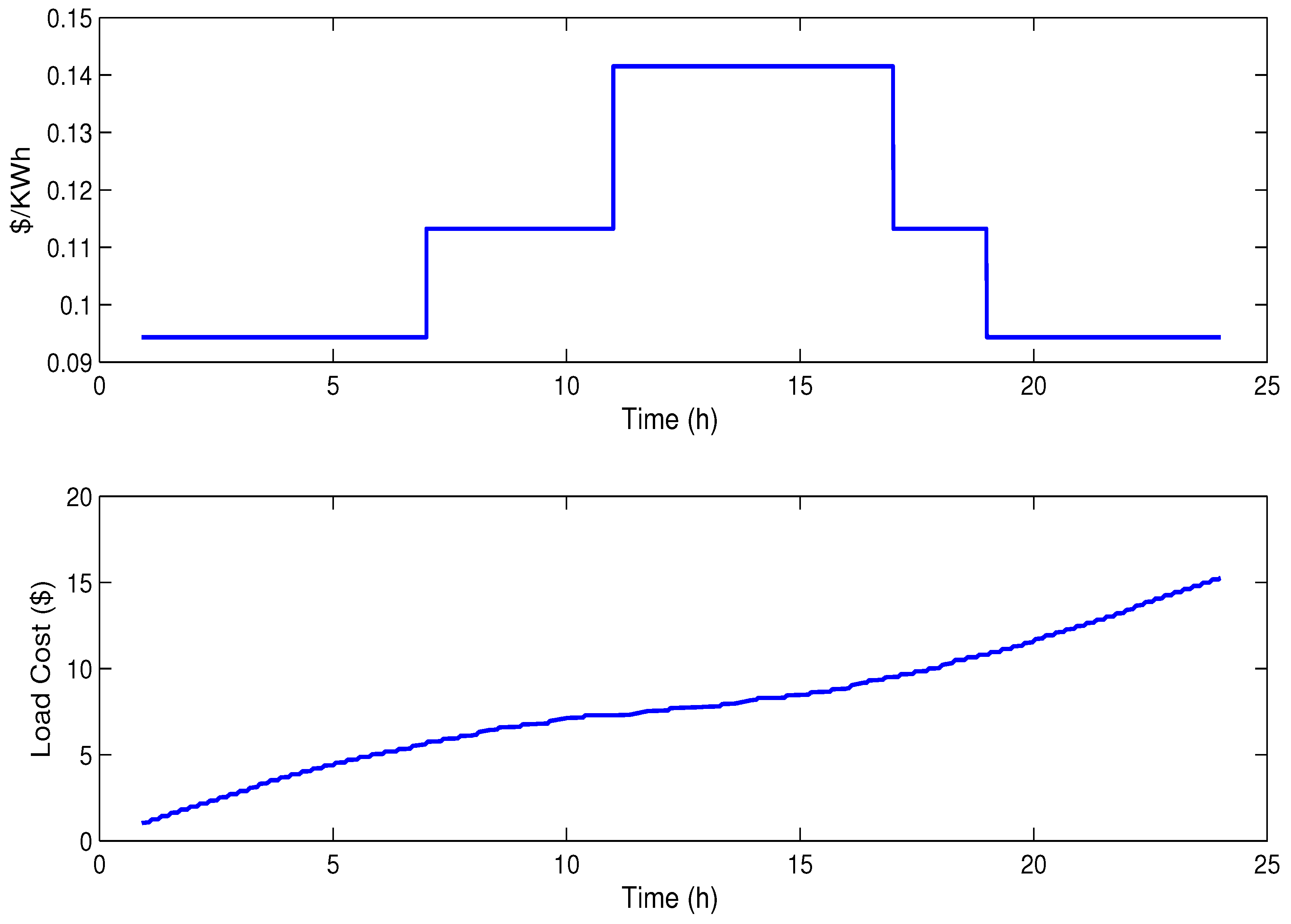
4.1. Case 1
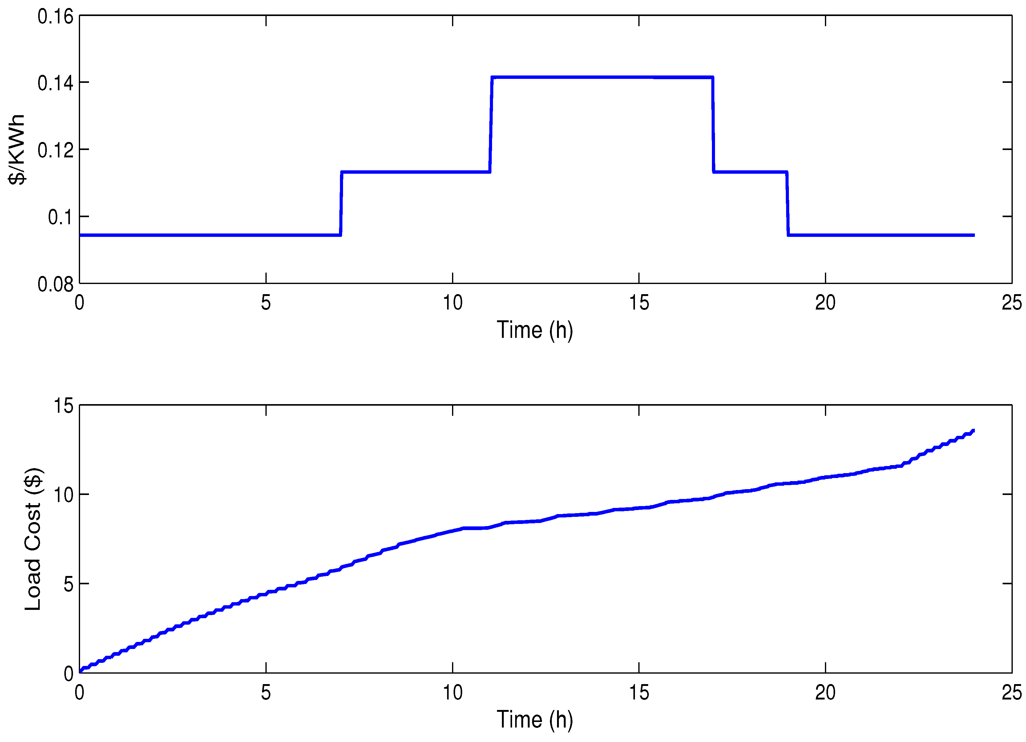
In case 1, baseline, regular and burst loads for the proposed system are run without any control or scheduling mechanism in order to find the total load for a day.
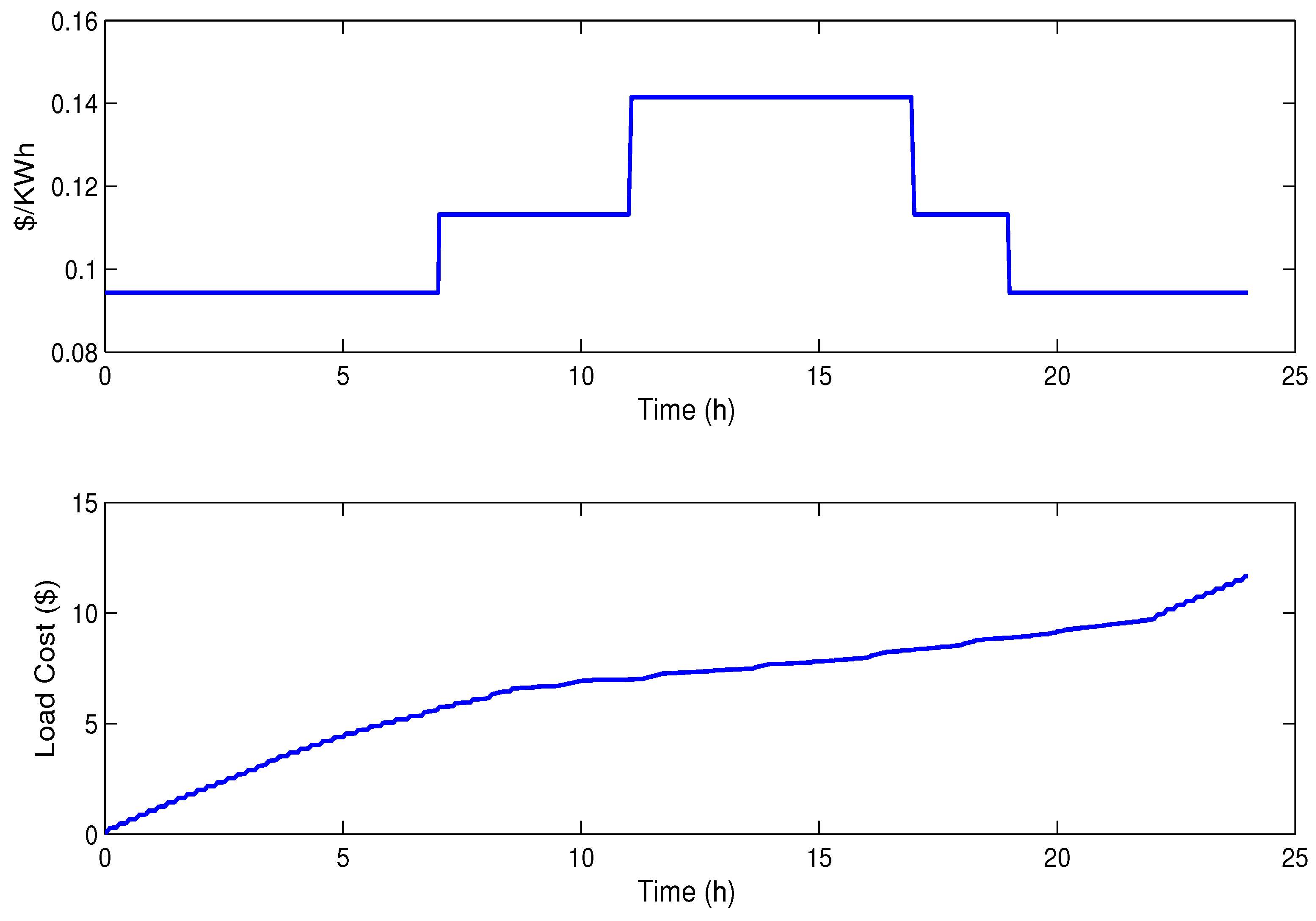
Figure 5 shows the total cost of unscheduled load and pricing scheme used, in which per unit prices of PKR 10/kWh (0.094 USD) for off-peak, PKR 12/kWh (0.113 USD) for mid peak and PKR 15/kWh (0.141 USD)for peak hours are used. We have used the conversion rate of 106 PKR equivalent to 1 USD.
Figure 6,
Figure 7,
Figure 8 and
Figure 9 show cost, power and temperature variation of HVAC, refrigerator, water heater and lighting, respectively. Total cost in this case is PKR 1692.3. (15.96 USD).
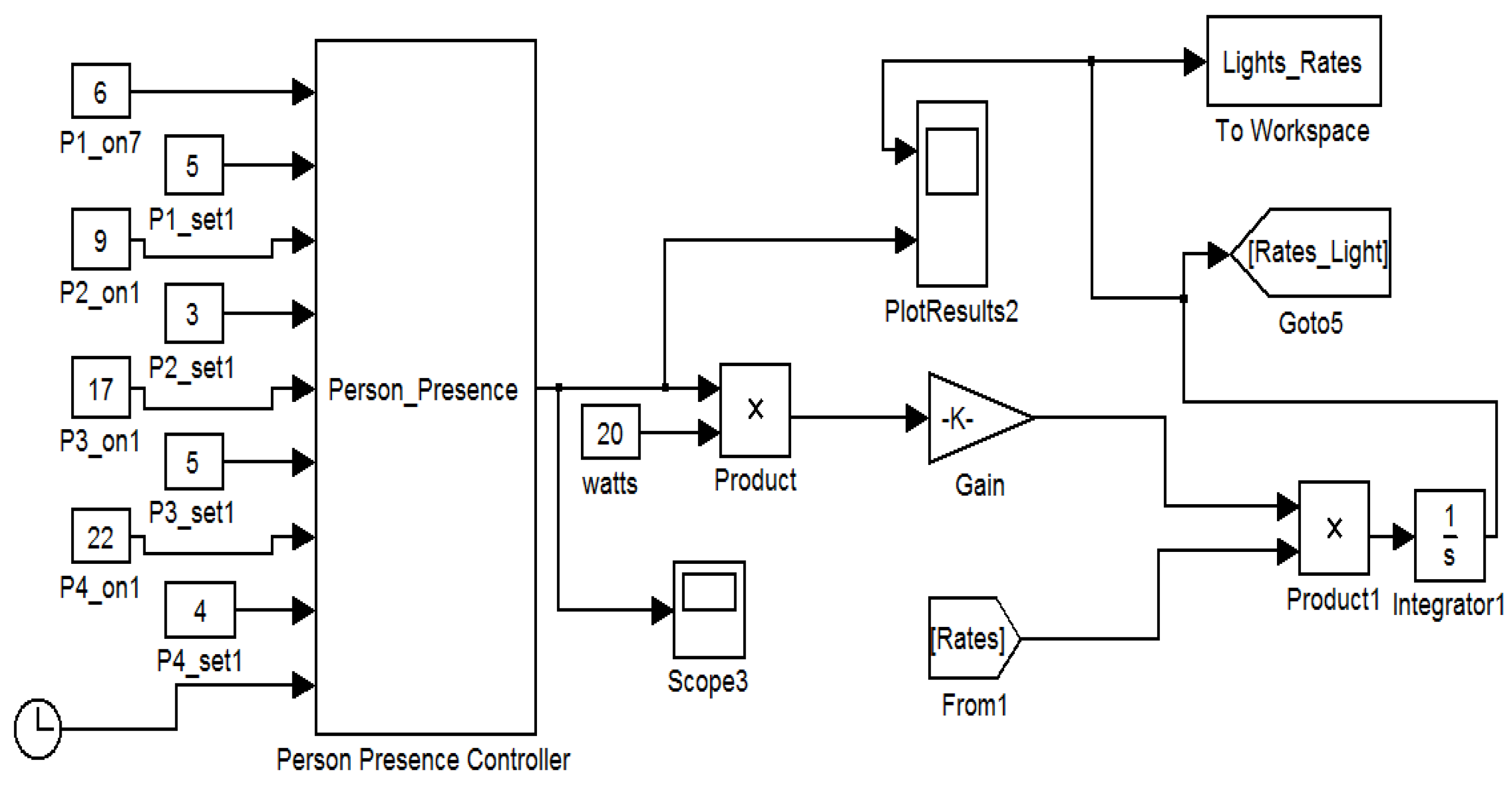
4.2. Case 2
In case 2, a strategy has been implemented to control the consumption of devices that are dependent on the number of persons present at home. In this case, PPC senses the presence of persons at home and controls home appliances accordingly. Lighting and hot water consumption are controlled with the help of PPC. The number of persons varies from three to five in different time slots. This technique is useful to minimize the cost and to enhance the system’s reliability.
Figure 10,
Figure 11,
Figure 12 and
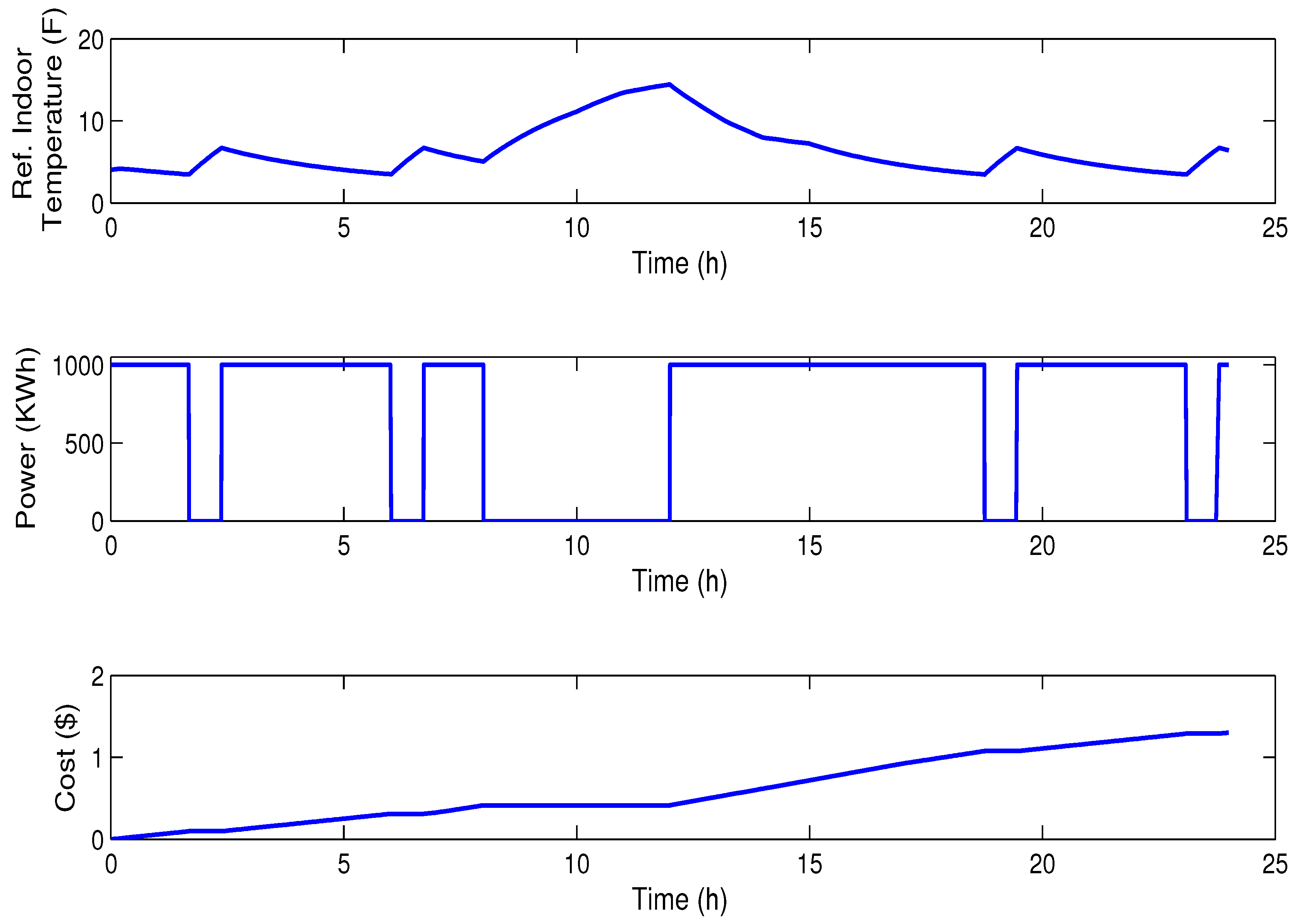
Figure 13 show the PPC, pricing scheme, HVAC cost and lighting cost, respectively. It is evident that the usage of PPC has reduced HVAC costs to PKR 1301.1 (12.27 USD). This provides a 22.9% savings in total cost.
4.3. Case 3
In case 3, PPC and a single Knapsack scheduling algorithm have been implemented together for further cost reduction in CHEMA.
Figure 14 shows the total consumption cost for case 3, which has now been reduced to PKR 1283.3 (12.14 USD).
4.4. Case 4
The focus of case 4 is to develop a system that schedules the loads in context of users’ comfort. Burst loads can only be operated at a scheduled time, otherwise the scheduler becomes ineffective, and the net cost will not be reduced as expected by the use of the scheduler. The parameter of User Comfort Index (UCI) is introduced to measure and ensure the user comfort. In UCI, the user has been provided with the flexibility to switch ON the desired burst load at any time according to his requirement; however, UCI asks users to provide some input about comfort level. The UCI is defined as the following:
By default, the settings for appliances are: HVAC 27
C, refrigerator 5
C and water heater is 55
C. When the scheduler is used to switch ON burst load, no change in these thresholds is required. When using the option of UCI, it is necessary to provide the required change in threshold levels to ensure the operation of burst load, which has now changed its priority and has become an essential load. There are some fixed slots in which the thresholds are relaxed automatically in order to implement the concept of flexible load categorization defined in
Section 3. Now, these appliances go to standby mode and new settings are updated which are: HVAC 23
C, refrigerator 10
C and water heater 45
C. These appliances will now be ON if the desired comfort is breached; otherwise, they will stay in standby mode till the burst load is switched OFF by the user.
Figure 15 shows the results of UCI.
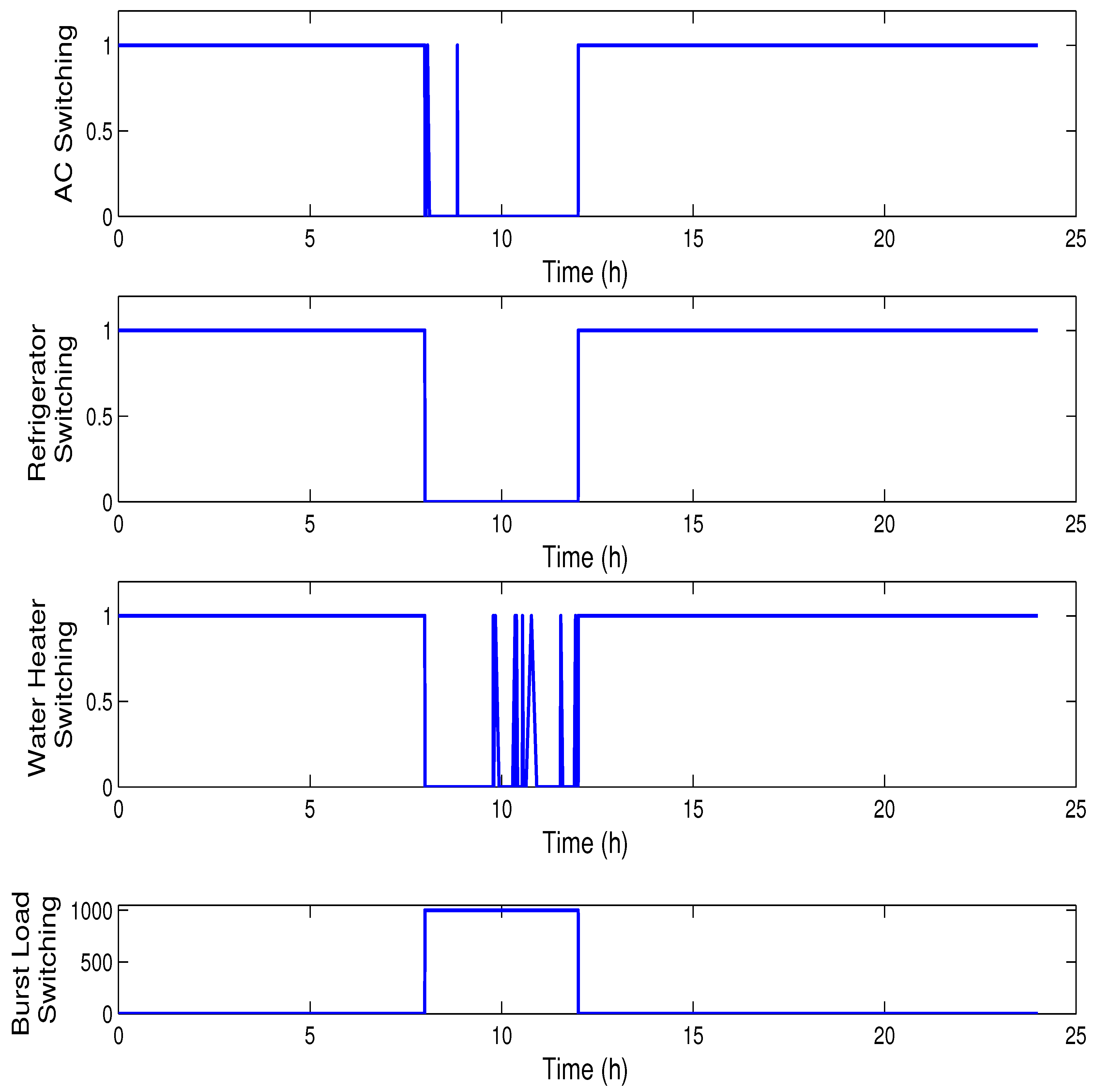
When the burst load is activated under UCI, the threshold of every appliance changes and it goes to standby mode. In
Figure 15, “1” stands for active and “0” stands for standby mode. The burst load is switched ON between 8:00 to 12:00 a.m. When burst load is activated, the threshold changes as depicted in
Figure 15. It is clearly seen that before 08:00 a.m., the threshold of the refrigerator was 5
C, but, after the activation of the burst load, the threshold has been changed. Switching the device to standby mode will provide the user an advantage, as in this mode, these appliances consume power almost equal to zero Watts. For instance, in
Figure 16, power consumed by the refrigerator during this period is almost negligible. It is the same case for the water heater and HVAC.
Table 2 shows total cost for load consumed for one day while carbon footprint results are tabulated in
Table 3.
4.5. Aggregated and Total Energy Consumption Results
This section is dedicated for discussion of aggregated energy consumption of five major modules used in four different cases of CHEMA. The section also includes a comparison of total energy consumption of the four cases.
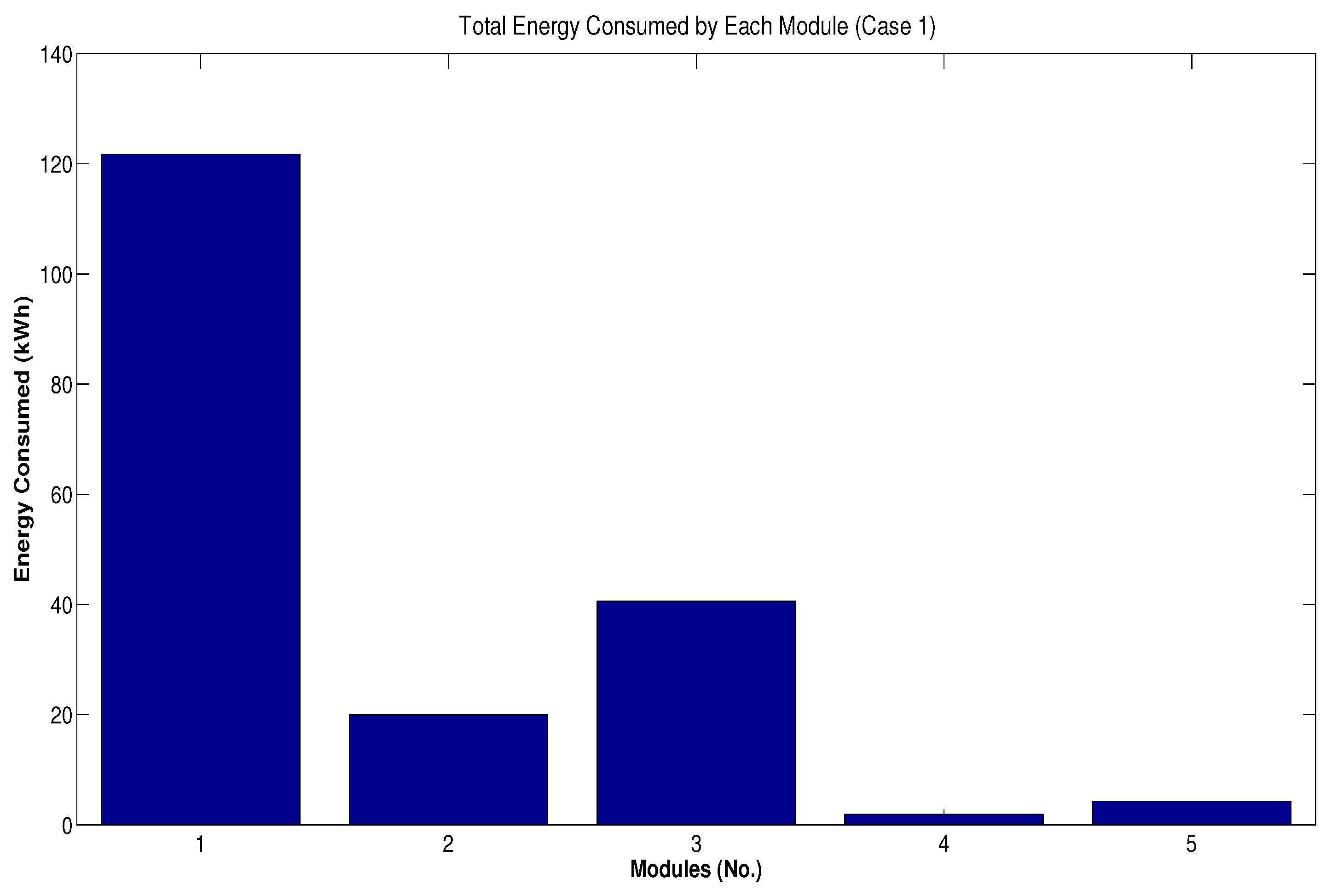
As discussed earlier, the five major modules include: space heating, refrigerator, water heater, lighting and burst load/scheduling module. Case one shows the operation of these modules without any scheduling or controlling technique except the use of regular load thermostats with predefined temperature settings. Aggregated energy consumption of five major modules for case one is shown in
Figure 17. In
Figure 17 and similar figures of following cases, modules 1 to 5 correspond to HVAC, refrigerator, water heater, lighting and burst load/scheduling modules, respectively. It is clearly seen that the highest consumption of energy is made by the space heating module (121.76 kWh) because of continuous usage and temperature limits. The minimum energy consumption corresponds to the lighting load, which is 1.92 kWh while total energy consumption for case one is calculated as 188.486 kWh.
The second case of the CHEMA is unscheduled load with PPC controller, and the strategy of PPC consists of two parts: one is the control of lighting load according to the presence of persons at home, and the second is the control of regular loads according to the forecasted consumption of water demand. The forecasting is based on the EPRI model. The basic purpose of the EPRI model is to control the consumption of energy according to demand and save the wastage of energy on basis of forecasted demand. Loads with thermal storage capacity are ideal for DSM and application of the EPRI model on a regular load is helpful in saving total energy consumption and ultimately a reasonable reduction in energy cost. The EPRI model has been designed on the basis of data collected by eleven different companies. Parameters recorded during collection of data include latitude, air temperature, water temperature,
etc. The model is based on strong statistical analysis, and it considers various categories of users along with the demographic and climatic factors. Initially, 16 variables were considered for the model, but, finally, the interdependent variables were dropped off and only 7 independent variables were included in the model. Results of the aggregated energy consumption of the second case are depicted in
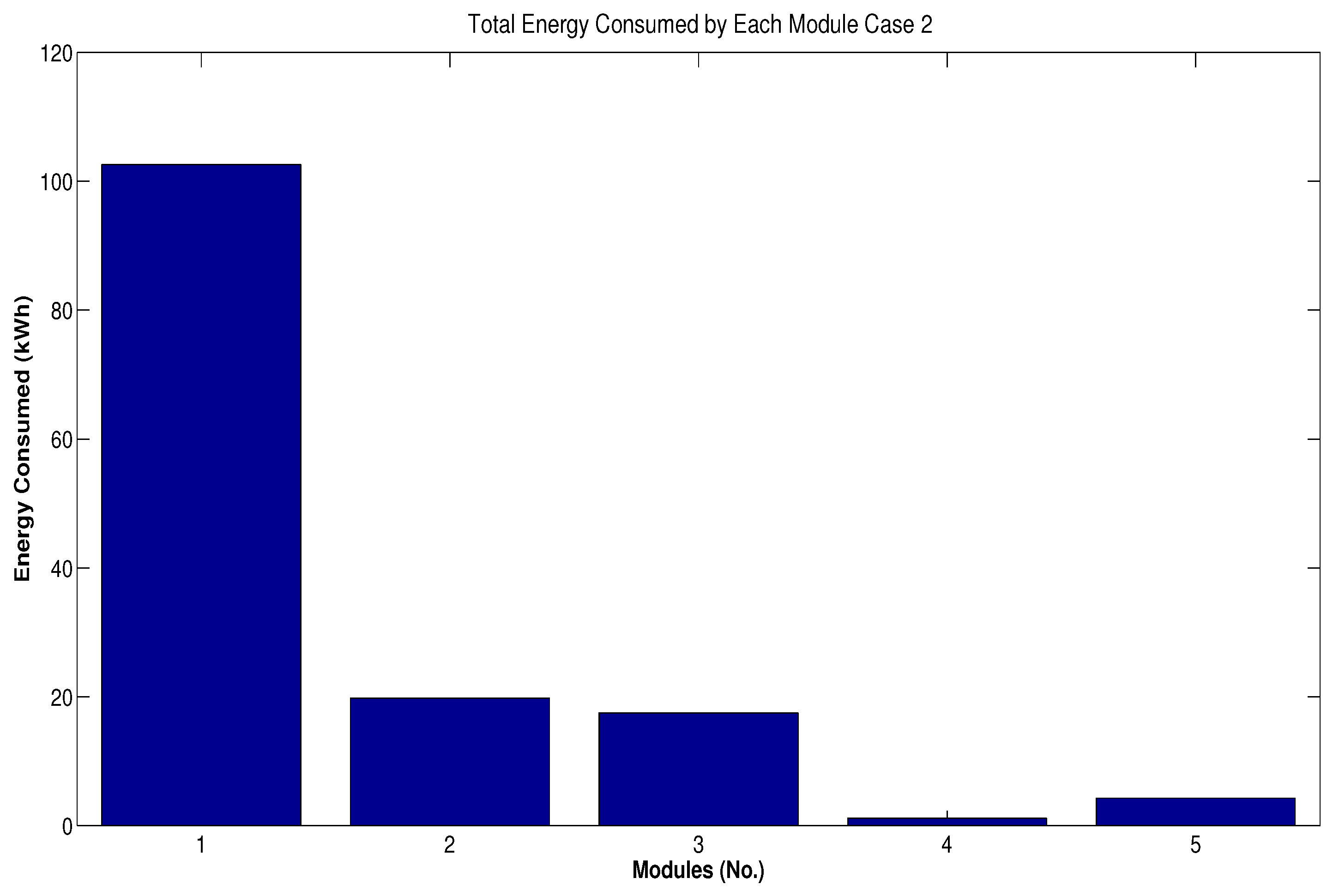
Figure 18.
Figure 18 reveals a reasonable reduction in consumption of the HVAC, water heater and lighting load which is 19.17 kWh, 23.08 kWh and 0.78 kWh, respectively. Second case corresponds to total energy consumption of 145.17 kWh.
The third case of CHEMA includes scheduling of burst loads. The scheduling is based on the single Knapsack algorithm, which is inspired from an example of a thief with a sack in a shop to decide optimally the weights and values of the items constrained to the total capacity of the sack. Results of the third case are shown in
Figure 19, and it can be seen that only a minor reduction in aggregated energy consumption and cost has been obtained. This is because of the fact that the total capacity of the burst load is limited to 4.28 kWh, which is merely 2% of the total regular load. Therefore, this case shows a reduction of 43.64 kWh energy consumption as compared to the first case and a further decrease of 0.33 kWh as compared to the second case.
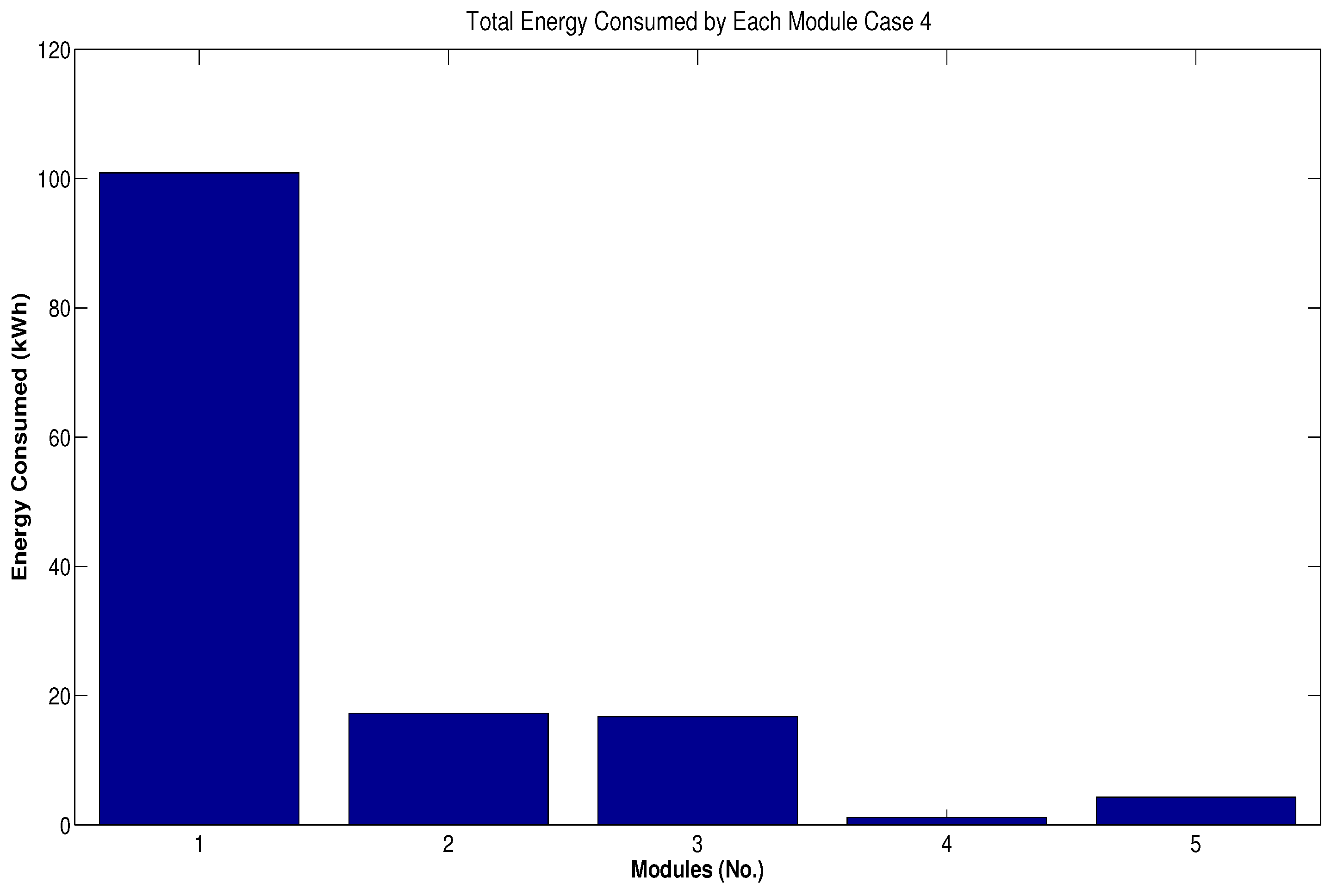
Case four of CHEMA has been designed in order to integrate the effects of users’ comfort in the energy cost minimization model. The basic idea is to relax the temperature threshold limits of the regular loads as described in Equation (12). The changing of threshold limits is subject to activation of burst loads. Results of case four are mentioned in
Figure 20. This case further reduces the aggregated energy consumption by 4.55 kWh by taking advantage of the regular loads’ temperature limit relaxation.
Total energy consumption of cases 1 to 4 is 188.486 kWh, 145.173 kWh, 144.84 kWh and 140.29 kWh, respectively. It is clearly seen that there is a visible and reasonable reduction in case 2 to case 4 as compared to case 1 while a little bit more reduction is also caused among cases 2 to 4 by application of different strategies. In summary, case 2 corresponds to 23.11%, case 3 to 24% and case 4 to 25.7% energy cost reduction as compared to case 1.
Table 4 shows the total energy consumption results of four cases.
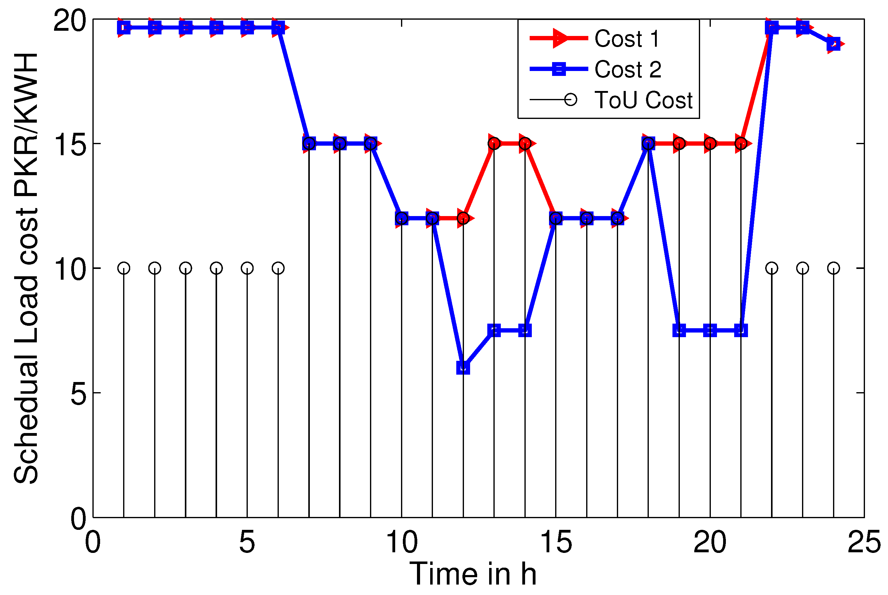
Our proposed model consists of six layers and has many unique features including the partial base line load concept. Regarding the energy cost minimization, the effect of the partial base line load is compared with the reference paper [
19].
Figure 21 shows the ToU pricing scheme, cost of the reference paper (Cost 1) and the CHEMA cost (Cost 2). The appliances’ ratings are taken as the same as the reference paper, and the base line load is assumed to be 1000 W, which is dealt with the Equation (
1).
It is clearly seen that, in peak hours, the cost of our proposed model is less than the reference paper.
5. Conclusions
In this paper, we have proposed CHEMA for home energy management with multiple appliance scheduling options for peak load reduction and users’ total energy cost minimization. UCI has also been included in CHEMA to ensure the least disturbance in users’ comfort. CHEMA has six layers, and four of these layers have been implemented in Simulink with embedded MATLAB code. Simulation results have shown the peak load reduction of 22.9% for unscheduled load with PPC, 23.15% for scheduled load with PPC and 25.56% for scheduled load with UCI. Similarly, total cost reduction of 23.11%, 24% and 25.7% has been observed, respectively. Aggregated energy consumption of various modules used in four cases has also been investigated. Results of energy consumption show total energy consumption of cases 1 to 4 is 188.486 kWh, 145.173 kWh, 144.84 kWh and 140.29 kWh, respectively. Implementation of the remaining two layers of CHEMA is planned in our future work.
Acknowledgments
The authors would like to extend their sincere appreciation to the Deanship of Scientific Research at king Saud University for funding this Research group No. 037-1435-RG.
Author Contributions
Anzar Mahmood and Nadeem Javaid proposed the main idea. Anzar Mahmood and Faisal Baig performed simulations. Nabil Alrajeh, Zahoor Ali Khan, Umar Qasim wrote the manuscript.
Conflicts of Interest
The authors declare no conflict of interest.
References
- Mahmood, A.; Javaid, N.; Khan, M.A.; Razzaq, S. An overview of load management techniques in smart grid. Int. J. Energy Res. 2015, 39, 1437–1450. [Google Scholar] [CrossRef]
- Mahmood, D.; Javaid, N.; Alrajeh, N.; Khan, Z.A. Umar qasim, imran ahmed, and manzoor ilahi, realistic scheduling mechanism for smart homes. Energies 2016, 9. [Google Scholar] [CrossRef]
- Ahmad, A.; Javaid, N.; Alrajeh, N.; Khan, Z.A.; Qasim, U.; Khan, A. A modified feature selection and artificial neural network-based day-ahead load forecasting model for a smart grid. Appl. Sci. 2015, 5, 1756–1772. [Google Scholar] [CrossRef]
- Mahmood, A.; Javaid, N.; Razzaq, S. A review of wireless communications for smart grid. Renew. Sustain. Energy Rev. 2015, 41, 248–260. [Google Scholar] [CrossRef]
- Fathabadi, H. Ultra high benefits system for electric energy saving and management of lighting energy in buildings. Energy Convers. Manag. 2014, 80, 543–549. [Google Scholar] [CrossRef]
- Jiang, B.; Farid, A.M.; Toumi, Y. Demand side management in a day-ahead wholesale market: A comparison of industrial and social welfare approaches. Appl. Energy 2015, 156, 642–654. [Google Scholar] [CrossRef]
- Yan, Y.; Qian, Y.; Sharif, H.; Tipper, D. A survey on smart grid communication infrastructures: Motivations, requirements and challenges. IEEE Commun. Surv. Tutor. 2013, 15, 5–20. [Google Scholar] [CrossRef] [Green Version]
- Mohsenian-Rad, A.-H.; Wong, V.W.; Jatskevich, J.; Schober, R. Optimal and autonomous incentive-based energy consumption scheduling algorithm for smart grid. In Proceedings of the Innovative Smart Grid Technologies (ISGT), Gaithersburg, MD, USA, 19–21 January 2010; pp. 1–6.
- Qureshi, W.A.; Nair, N.-K.C.; Farid, M.M. Impact of energy storage in buildings on electricity demand side management. Energy Convers. Manag. 2011, 52, 2110–2120. [Google Scholar] [CrossRef]
- Zhu, Q.; Han, Z.; Basar, T. A differential game approach to distributed demand side management in smart grid. In Proceedings of the 2012 IEEE International Conference on Communications (ICC), Ottawa, ON, Canada, 10–15 June 2012; pp. 3345–3350.
- Khan, M.A.; Javaid, N.; Mahmood, A.; Khan, Z.A.; Alrajeh, N. A generic demand-side management model for smart grid. Int. J. Energy Res. 2015, 39, 954–964. [Google Scholar] [CrossRef]
- Wang, J.J.; Wang, S. Wireless sensor networks for home appliance energy management based on zigbee technology. In Proceedings of the 2010 International Conference on Machine Learning and Cybernetics (ICMLC), Qingdao, China, 11–14 July 2010; pp. 1041–1046.
- Zhang, D.; Liu, S.; Papageorgiou, L.G. Fair cost distribution among smart homes with microgrid. Energy Convers. Manag. 2014, 80, 498–508. [Google Scholar] [CrossRef]
- Samadi, P.; Mohsenian-Rad, H.; Wong, V.W.; Schober, R. Tackling the load uncertainty challenges for energy consumption scheduling in smart grid. IEEE Trans. Smart Grid 2013, 4, 1007–1016. [Google Scholar] [CrossRef]
- Erol-Kantarci, M.; Mouftah, H.T. Using wireless sensor networks for energy-aware homes in smart grids. In Proceedings of the 2010 IEEE Symposium on Computers and Communications (ISCC), Riccione, Italy, 22–25 June 2010; pp. 456–458.
- Yoon, J.H.; Baldick, R.; Novoselac, A. Dynamic demand response controller based on real-time retail price for residential buildings. IEEE Trans. Smart Grid 2014, 5, 121–129. [Google Scholar] [CrossRef]
- Nguyen, H.K.; Song, J.B.; Han, Z. Distributed demand side management with energy storage in smart grid. IEEE Trans. Parallel Distrib. Syst. 2015, 26, 3346–3357. [Google Scholar] [CrossRef]
- Long, K.; Yang, Z. Model predictive control for household energy management based on individual habit. In Proceedings of the 2013 25th Chinese Control and Decision Conference (CCDC), Guiyang, China, 25–27 May 2013; pp. 3676–3681.
- Costanzo, G.T.; Zhu, G.; Anjos, M.F.; Savard, G. A system architecture for autonomous demand side load management in smart buildings. IEEE Trans. Smart Grid 2012, 3, 2157–2165. [Google Scholar] [CrossRef]
- Pratt, R.; Conner, C.; Richman, E.; Ritland, K.; Sandusky, W.; Taylor, M. Description of Electric Energy Use in Single-Family Residences in the Pacific Northwest; Office of Energy Resources, Bonneville Power Administration: Washington, DC, USA, 1989; p. 21.
- Erol-Kantarci, M.; Mouftah, H.T. Tou-aware energy management and wireless sensor networks for reducing peak load in smart grids. In Proceedings of the 2010 IEEE 72nd Vehicular Technology Conference Fall (VTC 2010-Fall), Ottawa, ON, Canada, 6–9 September 2010; pp. 1–5.
- Gran, R.J. Numerical Computing With Simulink, Volume 1: Creating Simulations; Society for Industrial and Applied Mathematics: Philadelphia, PA, USA, 2007. [Google Scholar]
- House Thermal Model. Available online: http://www.mathworks.com/help/simulink/examples/thermal model of a house.html (accessed on 28 May 2015).
- Paull, L.; MacKay, D.; Li, H.; Chang, L. Awater heater model for increased power system efficiency. In Proceedings of the Canadian Conference on Electrical and Computer Engineering, CCECE’09, St. John’s, NL, Canada, 3–6 May 2009; pp. 731–734.
- Anas, M.; Javaid, N.; Mahmood, A.; Raza, S.; Qasim, U.; Khan, Z.A. Minimizing electricity theft using smart meters in ami. In Proceedings of the 2012 Seventh International Conference on P2P, Parallel, Grid, Cloud and Internet Computing (3PGCIC), Victoria, BC, Canada, 12–14 November 2012; pp. 176–182.
- Ciabattoni, L.; Comodi, G.; Ferracuti, F.; Fonti, A.; Giantomassi, A.; Longhi, S. Multi-apartment residential microgrid monitoring system based on kernel canonical variate analysis. Neurocomputing 2015, 170, 306–317. [Google Scholar] [CrossRef]
- Carbon Print. Available online: http://en.wikipedia.org/wiki/Carbonfootprint2014 (accessed on 15 June 2015).
- Carbon Off-Setting. Available online: http://www.carbonneutral.com/resource-hub/carbon-offsetting-explained (accessed on 15 June 2015).
- Green Power. Available online: http://www.epa.gov/greenpower/pubs/calcmeth.htm (accessed on 15 June 2015).
Figure 1.
Proposed Comprehensive Home Energy Management Architecture (CHEMA).
Figure 1.
Proposed Comprehensive Home Energy Management Architecture (CHEMA).
Figure 2.
CHEMA flow chart.
Figure 2.
CHEMA flow chart.
Figure 3.
Time of Use (ToU) pricing scheme.
Figure 3.
Time of Use (ToU) pricing scheme.
Figure 4.
Heater subsystem.
Figure 4.
Heater subsystem.
Figure 5.
Pricing scheme and total unscheduled cost (case 1).
Figure 5.
Pricing scheme and total unscheduled cost (case 1).
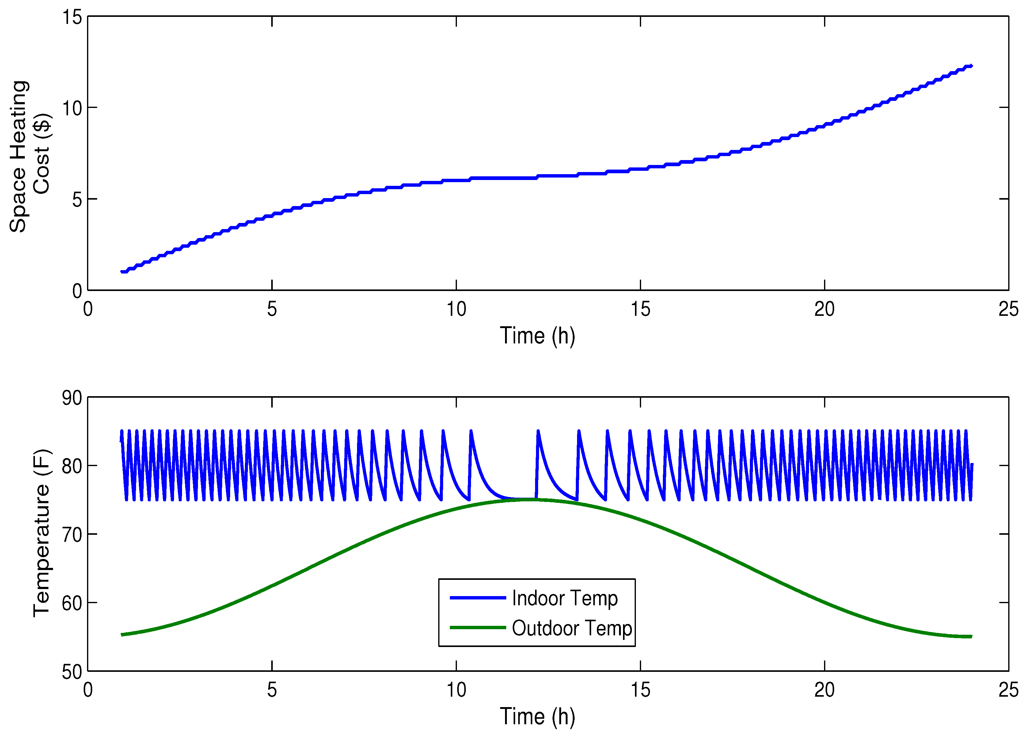
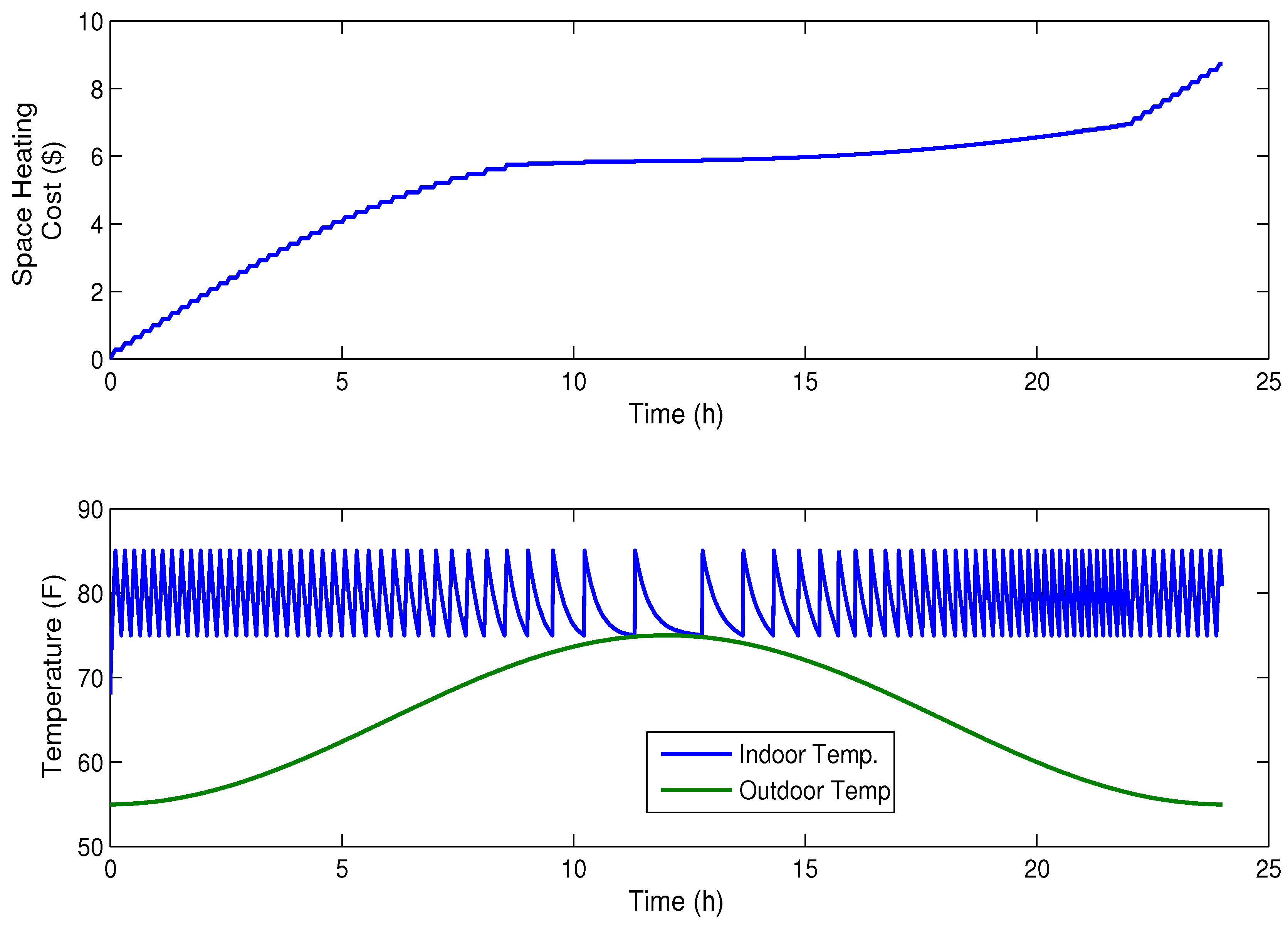
Figure 6.
Heating Ventilation Air Conditioning (HVAC) cost and temperature (case 1).
Figure 6.
Heating Ventilation Air Conditioning (HVAC) cost and temperature (case 1).
Figure 7.
Refrigeration cost, power and temperature variation (case 1).
Figure 7.
Refrigeration cost, power and temperature variation (case 1).
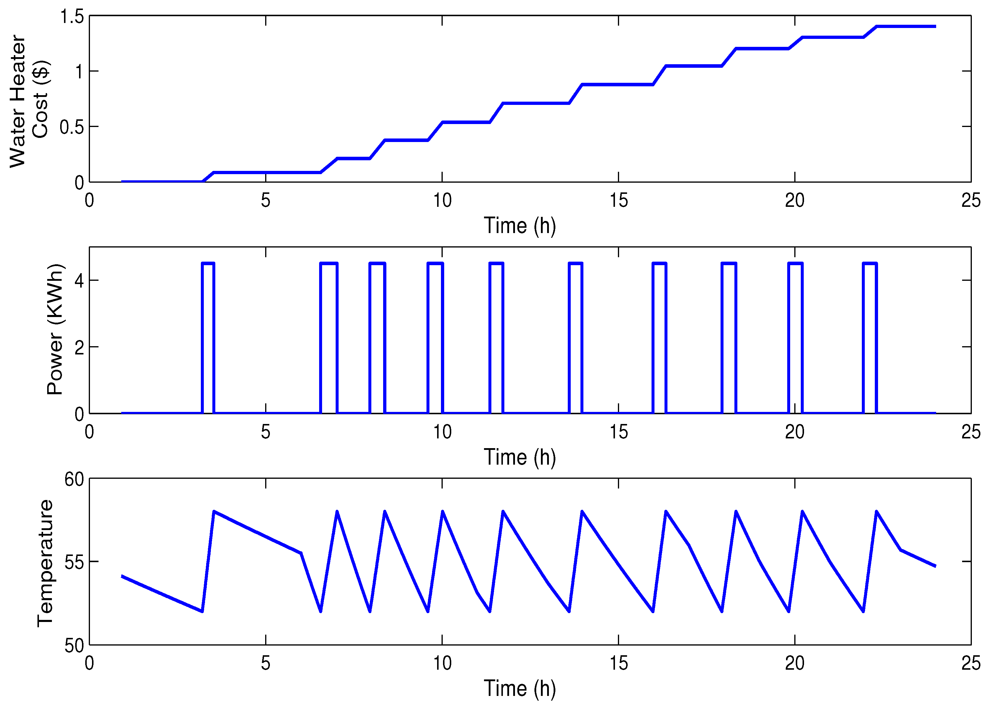
Figure 8.
Water heater cost, power and temperature variation (case 1).
Figure 8.
Water heater cost, power and temperature variation (case 1).
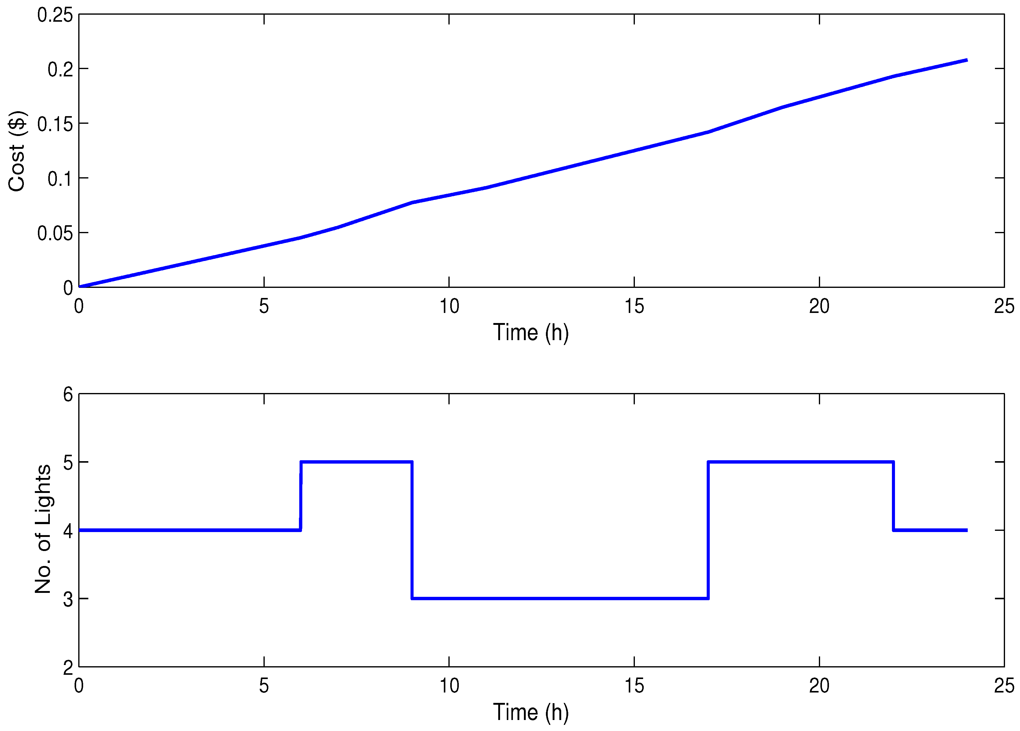
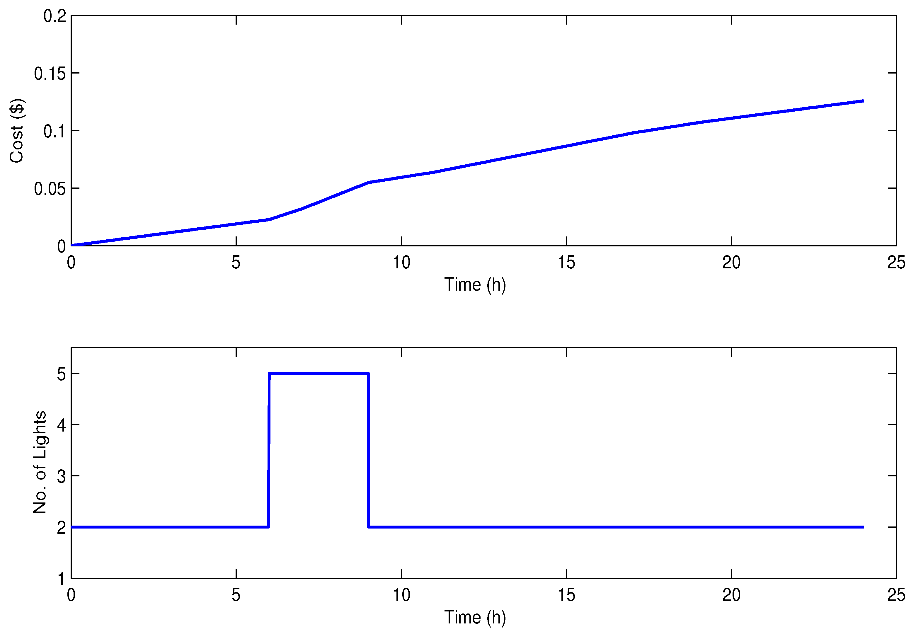
Figure 9.
No. of lights and cost variation (case 1).
Figure 9.
No. of lights and cost variation (case 1).
Figure 10.
Persons Presence Controller (PPC).
Figure 10.
Persons Presence Controller (PPC).
Figure 11.
Pricing scheme and total cost (case 2).
Figure 11.
Pricing scheme and total cost (case 2).
Figure 12.
HVAC cost and temperature variation (case 2).
Figure 12.
HVAC cost and temperature variation (case 2).
Figure 13.
Lighting cost (case 2).
Figure 13.
Lighting cost (case 2).
Figure 14.
Total cost (case 3).
Figure 14.
Total cost (case 3).
Figure 15.
User Comfort Index (UCI) results (case 4).
Figure 15.
User Comfort Index (UCI) results (case 4).
Figure 16.
Refrigeration cost (Case 4).
Figure 16.
Refrigeration cost (Case 4).
Figure 17.
Aggregated energy consumption (case 1).
Figure 17.
Aggregated energy consumption (case 1).
Figure 18.
Aggregated energy consumption (case 2).
Figure 18.
Aggregated energy consumption (case 2).
Figure 19.
Aggregated energy consumption (case 3).
Figure 19.
Aggregated energy consumption (case 3).
Figure 20.
Aggregated energy consumption (case 4).
Figure 20.
Aggregated energy consumption (case 4).
Figure 21.
Comparison of total energy consumption of four cases.
Figure 21.
Comparison of total energy consumption of four cases.
Table 1.
Green House Gase (GHG) Emission and Electricity Consumption Equivalency.
Table 1.
Green House Gase (GHG) Emission and Electricity Consumption Equivalency.
| Annual GHG Emission From | CO Emission From | Carbon Seized by |
|---|
| 2.9 passenger vehicles | 1552 gallons of gasoline consumed | 354 tree seedlings grown for 10 years |
| 32,836 miles/year driven by an average passenger vehicle | 14,813 pounds of coal burned | 11.3 acres of US forests in one year |
| 4.9 tons of waste sent to the land fill | 0.183 tanker trucks’ worth of gasoline | 0.106 acres of US forests preserved from conversion to cropland in one year |
| 0.707 Garbage trucks of waste recycled instead of landfilled | 32.1 barrels of oil consumed | Not Applicable |
Table 2.
Cost comparison of different cases.
Table 2.
Cost comparison of different cases.
| No. | Case | Total Cost (USD) |
|---|
| 1 | Unscheduled without PPC | 15.96 (1692.3 PKR) |
| 2 | Unscheduled with PPC | 12.27 ( 1301.1 PKR) |
| 3 | Scheduled with PPC | 12.14 ( 1286.3 PKR) |
| 4 | Load Flexibility (UCI) | 11.86 (1257.1 PKR) |
Table 3.
Carbon emission reduction of different cases.
Table 3.
Carbon emission reduction of different cases.
| No. | Case | Total Load (KWh/day) | CO Emission (Kg/day) |
|---|
| 1 | Unscheduled without PPC | 188.4860 | 126.2856 |
| 2 | Unscheduled with PPC | 145.1734 | 97.0429 |
| 3 | Scheduled with PPC | 144.8401 | 97.0429 |
| 4 | Load Flexibility (UCI) | 140.2925 | 93.9960 |
Table 4.
Load comparison of different cases.
Table 4.
Load comparison of different cases.
| No. | Case | Total Load (KWh/day) |
|---|
| 1 | Unscheduled without PPC | 188.4860 |
| 2 | Unscheduled with PPC | 145.1734 |
| 3 | Scheduled without PPC | 144.8401 |
| 4 | Load Flexibility (UCI) | 140.2925 |
© 2016 by the authors; licensee MDPI, Basel, Switzerland. This article is an open access article distributed under the terms and conditions of the Creative Commons Attribution (CC-BY) license (http://creativecommons.org/licenses/by/4.0/).


 ,
, 


