Hybrid Robust Control Law with Disturbance Observer for High-Frequency Response Electro-Hydraulic Servo Loading System

Abstract

Addressing the simulating issue of the helicopter-manipulating booster aerodynamic load with high-frequency dynamic load superimposed on a large static load, this paper studies the design of the robust controller for the electro-hydraulic loading system to realize the simulation of this kind of load. Firstly, the equivalent linear model of the electro-hydraulic loading system under assumed parameter uncertainty is established. Then, a hybrid control scheme is proposed for the loading system. This control scheme consists of a constant velocity feed-forward compensator, a robust inner loop compensator based on disturbance observer and a robust outer loop feedback controller. The constant velocity compensator eliminates most of the extraneous force at first, and then the double-loop cascade composition control strategy is employed to design the compensated system. The disturbance observer–based inner loop compensator further restrains the disturbances including the remaining extraneous force, and makes the actual plant tracking a nominal model approximately in a certain frequency range. The robust outer loop controller achieves the desired force-tracking performance, and guarantees system robustness in the high frequency region. The optimized low-pass filter Q(s) is designed by using the H∞ mixed sensitivity optimization method. The simulation results show that the proposed hybrid control scheme and controller can effectively suppress the extraneous force and improve the robustness of the electro-hydraulic loading system.

1. Introduction

The electro-hydraulic servo loading system is a hydraulic force (moment) control system which is used to apply the requested load to the actuating component or the manipulation component. For example, the experiment on the hydraulic booster in the helicopter-manipulating system needs this system. The hydraulic booster is in charge of transmitting the manipulation displacement signal and amplifying the manipulating force; meanwhile, it must respond to the driver’s command with high accuracy and fast speed under the high-frequency aerodynamic load. Through the electro-hydraulic loading system, which is employed to simulate the aerodynamic load on the ground, the control performance with the load of the booster can be evaluated, and this has vital significance in product performance experiments and improvement.

There are two types of loading: active and passive. The difficulty in the passive loading system is achieving the desired loading force on the condition of accompanying the motion of the loaded plant. There exists an unavoidable problem in such a loading system, namely how to restrain the motion disturbance (the so-called extraneous force [1]), which originates from the motion of the loaded plant. This disturbance seriously affects the force-tracking accuracy, reduces the closed-loop bandwidth of the loading system, and seriously causes gradation in the force control performance. Therefore, extraneous force suppression is the key issue to ensure the reliability and confidence level of the experiment.

As noted by Alleyne and Liu [2], for hydraulic loading systems, the tracking performance is limited by flow nonlinearity, parametric uncertainty, and motion disturbance, and cannot be guaranteed with a simple PID control algorithm. Thus, the online self-tuning fuzzy PID [3] and the grey predictor fuzzy PID [4] control algorithm were implemented, respectively. Robust control technologies, such as quantitative feedback theory (QFT) [5,6], the H∞ mixed sensitivity method [7], variable structure control [8,9], neural network control [10,11], and fractional order adaptive robust control [12] had been investigated for robust force tracking in the presence of disturbances and uncertainty. Focusing on nonlinear characteristics and parameter uncertainty, some nonlinear system control methods [13,14,15,16] had also been investigated. In the above studies, the extraneous force had been treated as a part of the loading error, and the force-tracking performance was obtained through feedback and feed-forward controllers.

From the forming mechanism of the extraneous force and the viewpoint of disturbance compensation, Liu [1] in China proposed a disturbance compensation method based on the structure invariance principle, actuator velocity was used to eliminate the actuator’s motion disturbance. This feed-forward compensation belongs to the direct disturbance compensation. Although it had made good elimination results in a low-frequency loading system, there were problems in physical implementation and velocity acquisition. Moreover, there is a lack of robustness against system uncertainty. In order to overcome the difficulty in acquiring velocity, a velocity synchronization method [17] was proposed, where the position input of the servo valve was alternatively utilized as a velocity signal to design the compensator. In view of improving the robustness of the compensation term, a hybrid control method [18] and dual-loop control [19] had further been proposed. Considering system uncertainties, the disturbance observer–based controller with a double-loop structure [20,21] was investigated. Problems of disturbance suppression and force tracking had been solved separately: the inner loop compensator was designed to restrain the disturbances and perturbations and to make the actual plant approximate the given nominal model, and the overall performance of the system was improved by the outer loop controller. So far, some compound control schemes combined with feed-forward compensation, such as double-loop cascade composition control [22], the nonlinear QFT technique [23], inverse model observer [24], adaptive control law [25], the H∞ method [26], and iterative learning [27], etc., had been put forward. The known studies show that force-tracking accuracy is limited by the extraneous force suppression level, especially in the presence of parameter perturbation. With the continuously increasing performance requirements for the loading system, it is difficult to obtain better tracking performance with a single approach, even if such an approach had made achievements in the low-frequency case.

The electro-hydraulic system is of high nonlinearity and parameter uncertainty. Nonlinearity mainly is caused by the flowrate-pressure characteristics of the servo valve, the compressibility of the hydraulic oil and the friction force of the hydraulic cylinder. A four-quadrant flowrate-pressure nonlinear model of the servo valve was established in [28,29,30,31]. Kemmetmüller and Kugi studied the impedance-based nonlinear control of the hydraulic servo system [28]. Scheidl and Manhartsgruber studied the singular issue in the mathematic model of the nonlinear hydraulic drive system, and proposed an approach of two subsystems with a boundary layer to analyze the nonlinear behavior [29]. Sun and Chiu studied the design of the nonlinear disturbance observer–based hydraulic force controller, and proposed the observer with a simple PI structure and a nonlinear control law based on the passivity theorem [30,31]. Currently, problems exist in the application of the above-mentioned nonlinear control approach in the force servo system, and the exact mathematical model of the servo valve is needed. Moreover, the robust control law, which is based on the Q-filter disturbance observer and the H∞ theory and does not rely on the exact mathematical model, can be easily designed. Therefore, this paper mainly studies the design method of this kind of control law.

This paper focuses on the high-frequency loading issue of an electro-hydraulic loading system with high-frequency dynamic load superimposed on a large static load of the helicopter- manipulating booster, and mainly studies a linear hybrid control scheme with a constant velocity feed-forward compensator and a double-loop cascade composition control strategy. The constant velocity compensator is designed to eliminate most of the extraneous force. The disturbance observer–based inner loop compensator restrains the disturbances, including the remaining extraneous force, and makes the actual plant tracking a nominal model approximately in a certain frequency range. The robust outer loop controller guarantees the desired force-tracking accuracy, and improves system robustness in the high-frequency region.

2. System Overview and Analysis

2.1. System Description

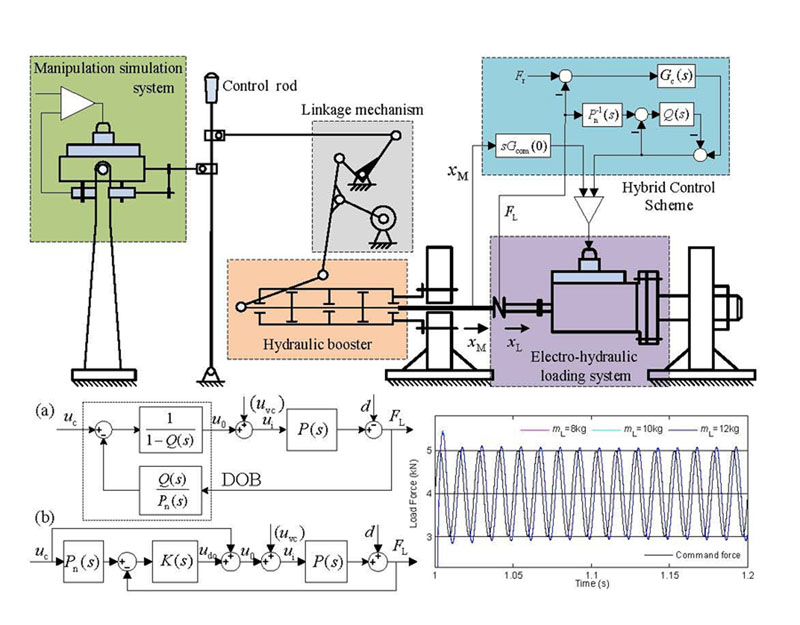
The helicopter-manipulating booster is a hydraulic position servomechanism with negative feedback. It is composed of three basic parts, a dispensing mechanism (slide valve), an actuator (piston) and a feedback mechanism (input rocker lever). In this valve-controlled hydraulic cylinder system, the displacement of the piston is controlled by the mechanical input of the rocker lever. The electro-hydraulic loading system is used to evaluate the control performance with the load of the booster on the ground, and its schematic diagram is depicted in Figure 1. The left block is a low-power electro-hydraulic position servo system, which is used to simulate the operating action on the control rod by the driver’s hand. The control rod is linked to the rocker lever of the booster by the linkage mechanism, and the rod’s action is reflected on the booster piston rod by amplifying the manipulating force. The right block is an electro-hydraulic loading system of the valve-controlled symmetrical hydraulic cylinder. The loading hydraulic cylinder piston rod is concatenated to the booster piston rod by a force sensor. The load spectrum is exerted on the booster when the loading hydraulic cylinder follows the motion of the booster. Symbols $x_{\mathrm{M}}$ and $x_{\mathrm{L}}$ represent the displacement of the booster piston and the loading hydraulic cylinder piston, respectively.

The studied electro-hydraulic loading system is characterized by high-frequency dynamic load superimposed on a large static load. The motion spectrum is compiled in sinusoidal form to simulate the operating actions on the control rod by hand, and its maximum frequency is 2 Hz. The load spectrum is compiled to simulate the aerodynamic load in the form of a sinusoidal dynamic load superimposed on a large static load, and the frequency range of the dynamic load is generally from 30 to 80 Hz. That is different from the loading system of the fixed-wing aircraft actuator, where the frequency of the load signal is equal to that of the actuator position signal. In the loading system of the helicopter booster, the frequency of the load spectrum is much greater than that of the booster motion, which results in the design of the controller of the loading system of the helicopter booster being more difficult than that of a fixed-wing aircraft actuator.

2.2. System Model and Analysis

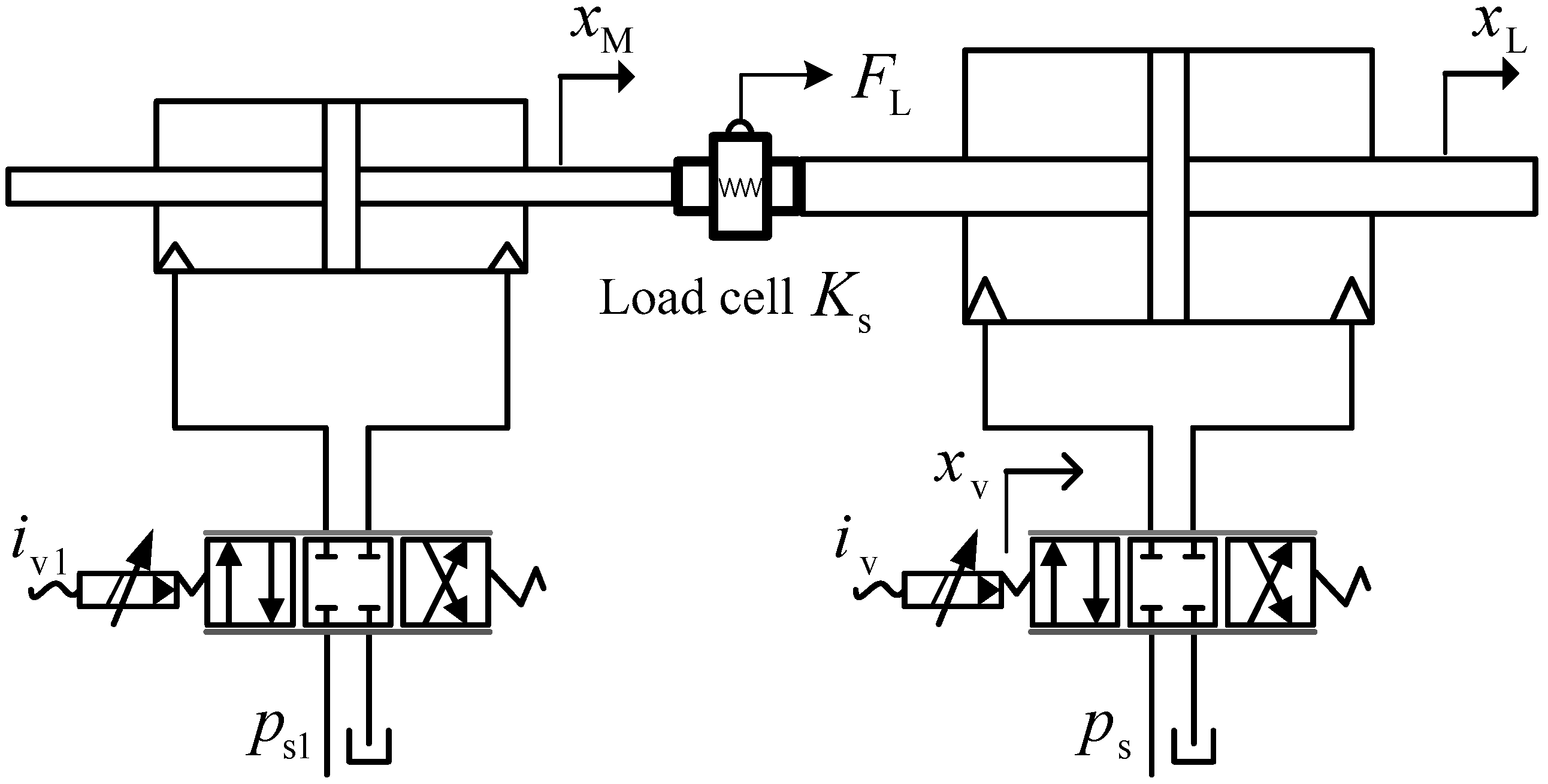
In this paper, we do not discuss the issue of the manipulation simulation of the booster. Hence, from the above descriptions of the manipulation simulation process, and to facilitate the study, the booster can be regarded as an electromagnetic valve controlled a hydraulic cylinder that is driven by the electromagnetic valve input. The studied equivalent schematic diagram is shown in Figure 2.

The mathematical model of the electro-hydraulic loading system can be set up by means of theoretical analysis or experiment identification. The theoretical model plays an important role in the design of controllers and the selection of system parameters.

As shown in Figure 2, the load force $F_{\mathrm{L}}$ (N) applied to the booster can be measured by the load cell, and in consideration of $K_{\mathrm{s}}$ (N/m), the elastic stiffness of the force sensor, it can be expressed as

$$F_{\mathrm{L}}=K_{\mathrm{s}}(x_{\mathrm{L}}-x_{\mathrm{M}}).$$

(1)

The load flow equation of the loading valve with ideal zero opening can be written as

$$q_{\mathrm{L}}=C_{\mathrm{d}}w{x}_{\mathrm{v}}\sqrt{(p_{\mathrm{s}}-\mathrm{sgn}(x_{\mathrm{v}})p_{\mathrm{L}})/\mathsf{\rho }},$$

(2)

where $x_{\mathrm{v}}$ is the spool displacement (m); $C_{\mathrm{d}}$ is the discharge coefficient; $w$ is the area gradient of the valve orifices (m); $\mathsf{\rho }$ is the oil density (kg/m³); $p_{\mathrm{s}}$ is the supply pressure (N/m²); $p_{\mathrm{L}}$ and $q_{\mathrm{L}}$ denote the load pressure (N/m²) and the load flow (m³/s), respectively.

In order to utilize linear system theory for dynamic analysis on the hydraulic power mechanism, to linearize Equation (2) yields the linearized load flowrate equation as

$$q_{\mathrm{L}}=K_{\mathrm{q}}{x}_{\mathrm{v}}-K_{\mathrm{c}}{p}_{\mathrm{L}},$$

(3)

where $K_q$ and $K_c$ are the linearized flow gain (m²/s) and flow-pressure coefficient (m⁵/(N·s)) of the servo valve around one operating point, respectively, $K_{\mathrm{q}}=C_{\mathrm{d}}w\sqrt{(p_{\mathrm{s}}-p_{\mathrm{L}})/\mathsf{\rho }}$ and $K_{\mathrm{c}}=C_{\mathrm{d}}w{x}_{\mathrm{v}}/(2\sqrt{(p_{\mathrm{s}}-p_{\mathrm{L}})\mathsf{\rho }})$. The values of $K_{\mathrm{q}}$ and $K_{\mathrm{c}}$ change with the variation of the operating points. When the valve opening is very small, the flowrate-pressure characteristics are determined by the leakage characteristics between the sleeve and the spool of the valve, and then $K_{\mathrm{c}}$ should be calculated by $K_{\mathrm{c}}=\mathsf{\pi }{r}_{\mathrm{c}}^{2}w/\left(32\mathsf{\mu }\right)$ according to the laminar flow formula.

The flowrate continuity equation of the hydraulic power mechanism can be expressed as

$$q_{\mathrm{L}}=A_{\mathrm{L}}\frac{d{x}_{\mathrm{L}}}{dt}+\frac{V_{\mathrm{L}}}{4{\mathsf{\beta }}_{\mathrm{e}}}\frac{d{p}_{\mathrm{L}}}{dt}+C_{\mathrm{sl}}{p}_{\mathrm{L}},$$

(4)

where $A_{\mathrm{L}}$ is the piston effective area(m²); ${\mathsf{\beta }}_{\mathrm{e}}$ is the fluid bulk modulus (N/m²); $C_{\mathrm{sl}}$ is the total leakage coefficient of the hydraulic cylinder (m⁵/(N·s)); and $V_{\mathrm{L}}$ represents the total control volume of the loading system (m³).

The force equilibrium equation for the loading hydraulic cylinder piston is

$$A_{\mathrm{L}}{p}_{\mathrm{L}}=m_{\mathrm{L}}\frac{d^2{x}_{\mathrm{L}}}{d{t}^2}+B_{\mathrm{L}}\frac{d{x}_{\mathrm{L}}}{dt}+F_{\mathrm{L}},$$

(5)

where $m_{\mathrm{L}}$ is the equivalent load mass (kg) including the mass of the piston, rods, force sensor and the load; and $B_{\mathrm{L}}$ represents the equivalent viscous damping coefficient (N·s/m).

Combining and solving Equations (1) and (3)–(5), the transfer function of the output load force $F_{\mathrm{L}}$, with the valve spool displacement $x_{\mathrm{v}}$ as the input and the displacement $x_{\mathrm{M}}$ of the loaded booster as the disturbance, can be derived as follows

$$F_{\mathrm{L}}(s)=G_{\mathrm{p}}(s)X_{\mathrm{v}}(s)-G_{\mathrm{d}}(s)s{X}_{\mathrm{M}}(s)=\frac{N_{\mathrm{U}}(0)}{P_{\mathrm{D}}(s)}{X}_{\mathrm{v}}(s)-\frac{N_{\mathrm{D}}(s)}{P_{\mathrm{D}}(s)}s{X}_{\mathrm{M}}(s),$$

(6)

where $K_{\mathrm{tm}}=K_c+C_{\mathrm{sl}}$; $N_{\mathrm{D}}\left(s\right)=\frac{V_{\mathrm{L}}{m}_{\mathrm{L}}}{4{\mathsf{\beta }}_{\mathrm{e}}{K}_{\mathrm{tm}}}{s}^2+\left(m_{\mathrm{L}}+\frac{V_{\mathrm{L}}{B}_{\mathrm{L}}}{4{\mathsf{\beta }}_{\mathrm{e}}{K}_{\mathrm{tm}}}\right)s+B_{\mathrm{L}}+\frac{A_{\mathrm{L}}^2}{K_{\mathrm{tm}}}$; $N_{\mathrm{U}}(0)=A_{\mathrm{L}}{K}_{\mathrm{q}}/K_{\mathrm{tm}}$; $P_{\mathrm{D}}\left(s\right)=\frac{V_{\mathrm{L}}{m}_{\mathrm{L}}}{4{\mathsf{\beta }}_{\mathrm{e}}{K}_{\mathrm{tm}}{K}_{\mathrm{s}}}{s}^3+\left(\frac{m_{\mathrm{L}}}{K_{\mathrm{s}}}+\frac{V_{\mathrm{L}}{B}_{\mathrm{L}}}{4{\mathsf{\beta }}_{\mathrm{e}}{K}_{\mathrm{tm}}{K}_{\mathrm{s}}}\right)s^2+\left(\frac{B_{\mathrm{L}}}{K_{\mathrm{s}}}+\frac{A_{\mathrm{L}}^2}{K_{\mathrm{tm}}{K}_{\mathrm{s}}}+\frac{V_{\mathrm{L}}}{4{\mathsf{\beta }}_{\mathrm{e}}{K}_{\mathrm{tm}}}\right)s+1$; $X_{\mathrm{v}}(s)$ and $X_{\mathrm{M}}(s)$ denote the Laplace transform of $x_{\mathrm{v}}$ and $x_{\mathrm{M}}$, respectively.

It can be noticed from Equation (6) that, besides the valve spool displacement $x_{\mathrm{v}}$, $F_{\mathrm{L}}$ is related to the booster displacement $x_{\mathrm{M}}$ as well. The latter motion disturbance exactly results in the extraneous force in the loading system.

The spool movement dynamics of the loading valve cannot be ignored within the bandwidth of our studied loading system. And a second-order dynamic equation is therefore utilized to describe the relationship between the coil current input $i_{\mathrm{v}}$ (A) and the spool displacement $x_{\mathrm{v}}$, as it can well reflect the valve spool dynamics at high frequencies, and its transfer function can be expressed as

$$G_{\mathrm{v}}(s)=\frac{X_{\mathrm{v}}(s)}{I_{\mathrm{v}}(s)}=\frac{K_{\mathrm{v}}{\mathsf{\omega }}_{\mathrm{v}}^2}{s^2+2{\mathsf{\zeta }}_{\mathrm{v}}{\mathsf{\omega }}_{\mathrm{v}}s+{\mathsf{\omega }}_{\mathrm{v}}^2}$$

(7)

where $I_{\mathrm{v}}(s)$ is the Laplace transform of $i_{\mathrm{v}}$; $K_{\mathrm{v}}$ is the valve spool position gain (m³/(A·s)); ${\mathsf{\omega }}_{\mathrm{v}}$ and ${\mathsf{\zeta }}_{\mathrm{v}}$ are the natural frequency (rad/s) and the damping ratio of the loading valve, respectively.

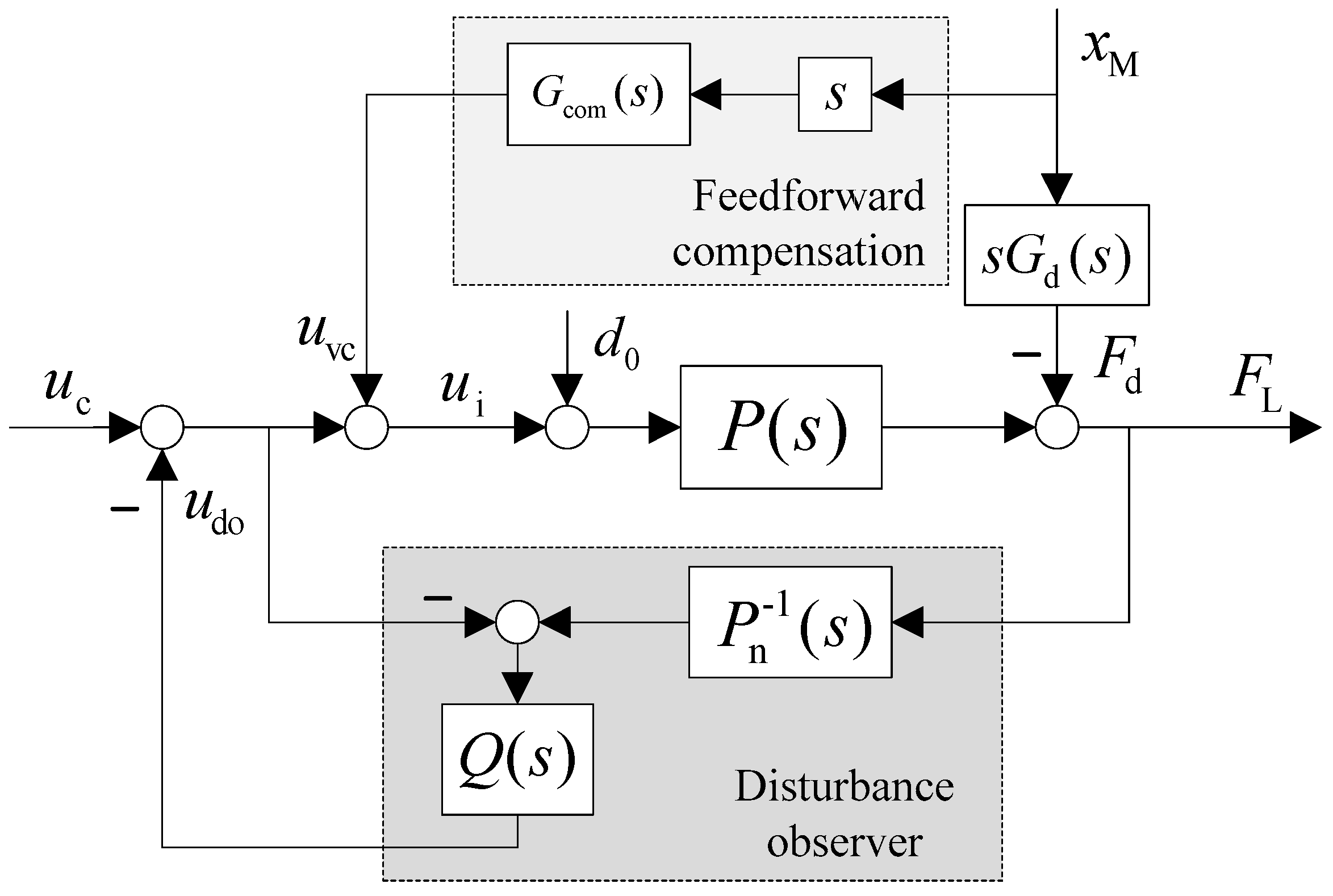
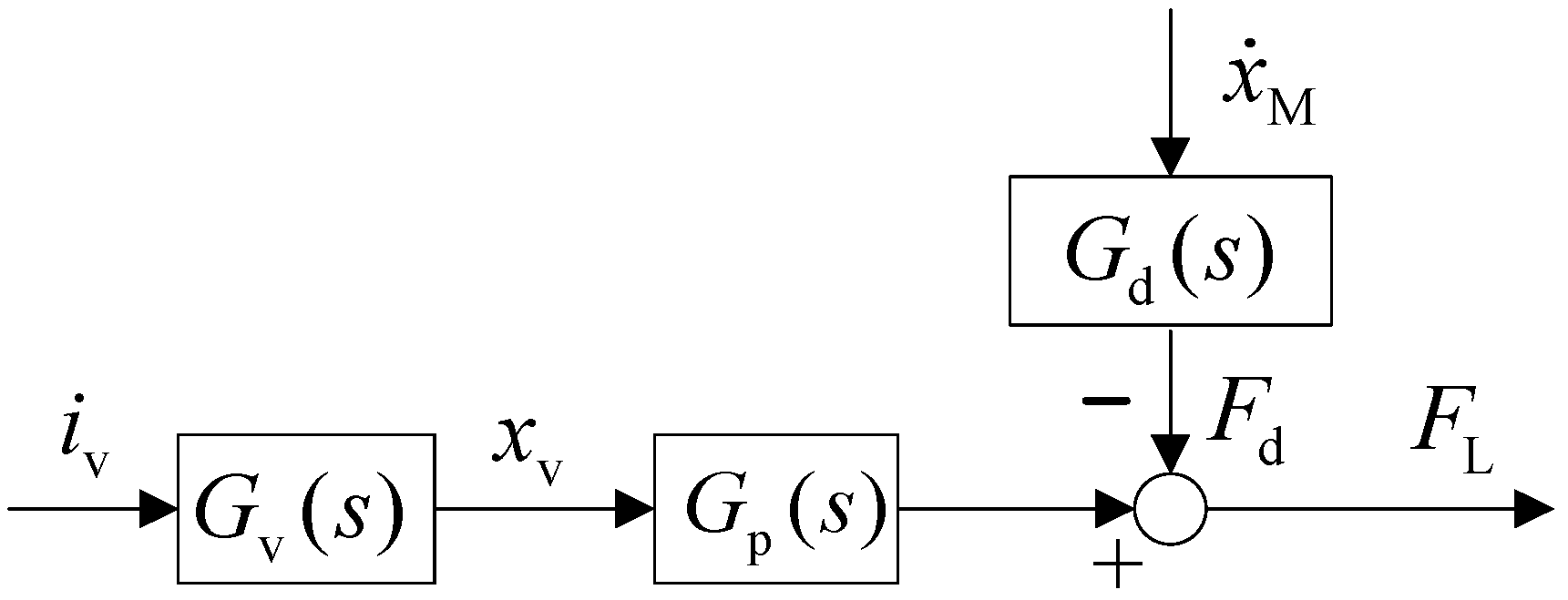
Therefore, a simplified block diagram of the loading system can be drawn in Figure 3, where $F_{\mathrm{d}}$ is the output disturbance force from the motion of the loaded plant and $F_{\mathrm{d}}=G_{\mathrm{d}}(s)s{X}_{\mathrm{M}}$.

2.3. Equivalent Linear Model Set

Normally, we linearize the flow quantity equation of the valve around the neutral position, because the general hydraulic servo system is often working around that, and $K_{\mathrm{q}}$ and $K_{\mathrm{c}}$ are obtained as fixed constants. However, for the hydraulic loading system with strong position interference, its operating point varies over a large range. If the loading system is just described by a linear plant with linear parameters around one operating point, it is only possible to approximate the system dynamics over a limited region of operation. Moreover, parameter uncertainty in some hydraulic systems is inevitable and this can degrade the closed-loop performance. In particular, with the requirement of high closed-loop bandwidth (80 Hz), the inaccurately described system leads to unreliable design. Therefore, any single linear time invariant (LTI) model cannot describe the whole system’s dynamics, and it is necessary to establish a set of equivalent LTI models that describe the dynamics of the nonlinear hydraulic system over the whole envelope of operation.

From the design point of view, we believe that the transfer function $G_{\mathrm{v}}(s)$ can accurately reflect the dynamic characteristics of the servo valve, and some structural parameters, such as $V_{\mathrm{L}}$, $A_{\mathrm{L}}$, $K_{\mathrm{s}}$, etc., can be precisely measured and kept constant. However, the equivalent load mass $m_{\mathrm{L}}$, which is described by the lumped mass method, is difficult to measure precisely, and the fluid bulk modulus ${\mathsf{\beta }}_{\mathrm{e}}$ fluctuates with fluid temperature and mixed air. According to the maximum load demand of the booster with some appropriate margin (from −11 to 22 kN), the initial boundaries of $K_{\mathrm{q}}$ and $K_{\mathrm{c}}$ can be calculated. The electro-hydraulic loading system generally uses the servo valve with zero opening or positive opening, and even the zero-opening servo valve generally also has a very small positive opening (under-lapped). The positive opening and the variation of oil supply pressure $p_{\mathrm{s}}$ also result in the perturbations of $K_{\mathrm{q}}$ and $K_{\mathrm{c}}$. A lumped perturbation range can be obtained by integrating these perturbations into the initial boundaries of $K_{\mathrm{q}}$ and $K_{\mathrm{c}}$. Then, taking into account the leakage of the whole system can get the boundary of $K_{\mathrm{tm}}$.

Table 1. Parameters of the loading system.

Parameter	Value	Unit
Supply pressure $p_{\mathrm{s}}$	18–21	MPa
Piston effective area $A_{\mathrm{L}}$	24.63	cm2
Total control volume $V_{\mathrm{L}}$	4.5	cm3
Equivalent load mass $m_{\mathrm{L}}$	8–12	kg
Fluid bulk modulus ${\mathsf{\beta }}_{\mathrm{e}}$	700–1100	MPa
Viscous damping coefficient $B_{\mathrm{L}}$	800	N·s/m
Force sensor stiffness $K_{\mathrm{s}}$	100	kN/mm
Valve flow gain $K_{\mathrm{q}}$	2.92–3.85	m2/s
Total flow-pressure coefficient $K_{\mathrm{tm}}$	7 × 10−2 –7.5 × 10−2	cm5/(N·s)
Valve gain $K_{\mathrm{v}}$	0.3/20	mm/mA
Valve natural frequency ${\mathsf{\omega }}_{\mathrm{v}}$	200	Hz
Valve damping ratio ${\mathsf{\zeta }}_{\mathrm{v}}$	0.7	-
Feedback gain $K_{\mathrm{a}}$	4 × 10−4	mA/N

lists all the measured and calculated values of the parameters of the loading system.

From the model derived above, the loading system is a fifth-order system with motion disturbance and variable parameters. The denominator polynomial $P_{\mathrm{D}}(s)$ of $G_{\mathrm{P}}(s)$ can be expressed as follows

$$P_{\mathrm{D}}\left(s\right)=\left(\frac{s}{{\mathsf{\omega }}_{\mathrm{L}}}+1\right)\left(\frac{s^2}{{\mathsf{\omega }}_{\mathrm{h}}^2}+\frac{2{\mathsf{\xi }}_{\mathrm{h}}}{{\mathsf{\omega }}_{\mathrm{h}}}s+1\right)$$

(8)

where ${\mathsf{\omega }}_{\mathrm{L}}$ is the cutoff frequency of the inertial term and ${\mathsf{\omega }}_{\mathrm{L}}=K_{\mathrm{tm}}{K}_{\mathrm{h}}{K}_{\mathrm{s}}/[A_{\mathrm{L}}^2(K_{\mathrm{h}}+K_{\mathrm{s}})]$; ${\mathsf{\omega }}_{\mathrm{h}}$ and ${\mathsf{\xi }}_{\mathrm{h}}$ are the second-order oscillation frequency and the damping ratio of the force loop, respectively; ${\mathsf{\omega }}_{\mathrm{h}}={\mathsf{\omega }}_0\sqrt{(K_{\mathrm{h}}+K_{\mathrm{s}})/K_{\mathrm{h}}}$; $K_{\mathrm{h}}=4{\mathsf{\beta }}_{\mathrm{e}}{A}_{\mathrm{L}}^2/V_{\mathrm{L}}$ is the liquid spring stiffness, ${\mathsf{\omega }}_0=\sqrt{4{\mathsf{\beta }}_{\mathrm{e}}{A}_{\mathrm{L}}^2/(V_{\mathrm{L}}{m}_{\mathrm{L}})}$ represents the natural angular frequency of the hydraulic cylinder; ${\mathsf{\xi }}_{\mathrm{h}}$ can be calculated, but the symbolic representation is difficult to obtain.

After some calculation, the loading system $P(s)$ can be represented as an equivalent linear model set $P_0(s)$ having four uncertain parameters as

$$P(s)\in P_0(s)=\left\{\frac{K_{\mathrm{op}}{G}_{\mathrm{v}}(s)}{\left(\frac{s}{{\mathsf{\omega }}_{\mathrm{L}}}+1\right)\left(\frac{s^2}{{\mathsf{\omega }}_{\mathrm{h}}^2}+\frac{2{\mathsf{\xi }}_{\mathrm{h}}}{{\mathsf{\omega }}_{\mathrm{h}}}s+1\right)}\right\}$$

(9)

where ${\mathsf{\omega }}_{\mathrm{L}}\in [31.62,46.03]$; ${\mathsf{\omega }}_{\mathrm{h}}\in [3387,4464]$; ${\mathsf{\xi }}_{\mathrm{h}}\in [0.012,0.015]$; and $K_{\mathrm{op}}\in [9.56\times {10}^8,1.354\times {10}^9]$. In light of the statistics of the hydraulic servo system, the damping ratio of the hydraulic servo system is generally more than 0.1, and therefore we take ${\mathsf{\xi }}_{\mathrm{h}}=0.1$.

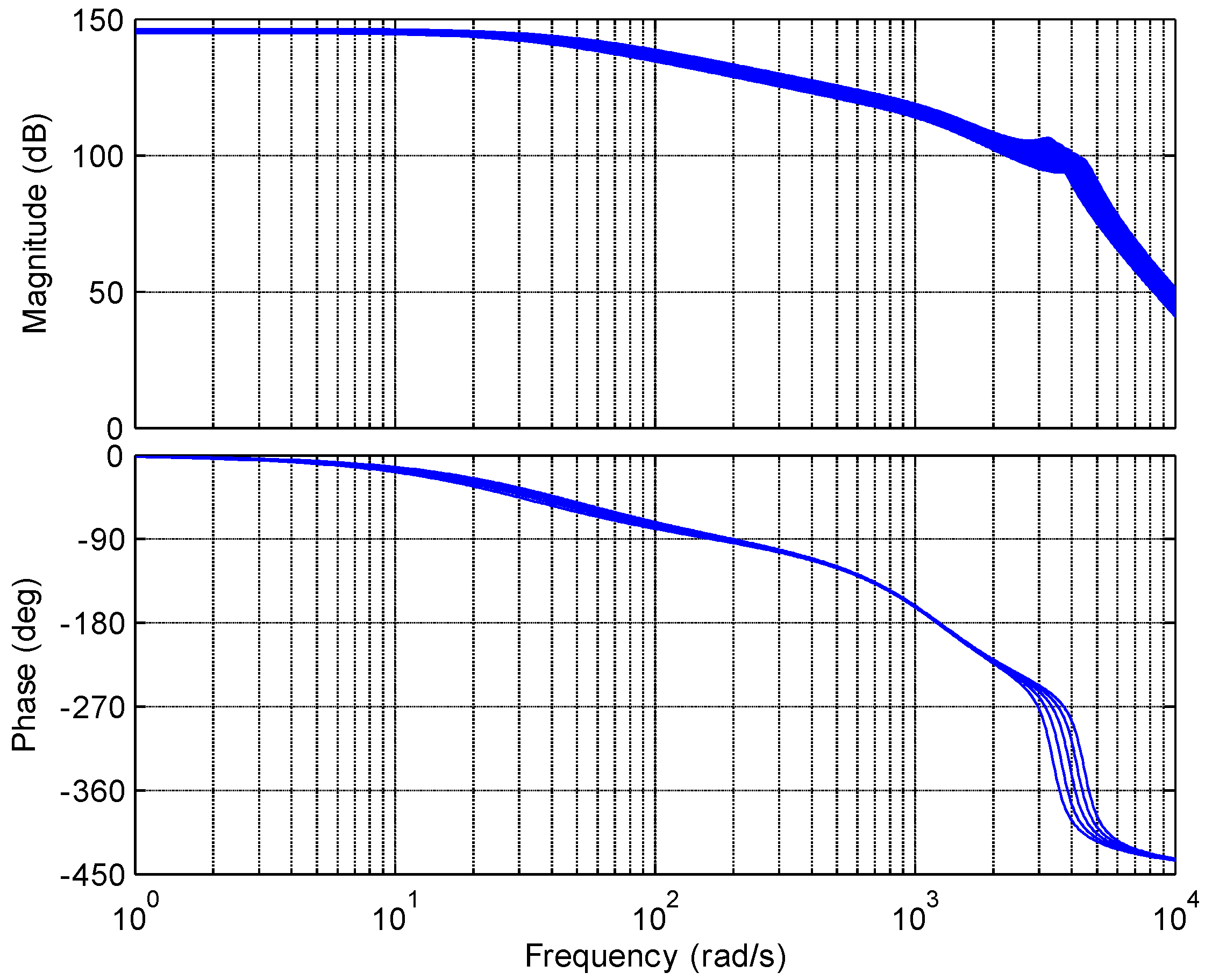
From the frequency characteristics of the equivalent model set in Figure 4, the dynamic characteristics of the loading system can be described by the linearized equivalent model set, but this equivalent method introduces a significant amount of dynamic uncertainty in the low-frequency region, which is smaller in the actual plant.

2.4. Disturbance Force Analysis

It is known from Equation (6) that the output loading force $F_{\mathrm{L}}$ consists of two parts: one part $F_{\mathrm{v}}=G_{\mathrm{p}}(s)X_{\mathrm{v}}(s)$ is controlled by regulating the spool displacement $x_{\mathrm{v}}$, and the other $F_{\mathrm{d}}$ results from the displacement $x_{\mathrm{M}}$ of the loaded plant. This disturbance force $F_{\mathrm{d}}$ is inevitably produced because of the motion of the loaded plant. The amount of $F_{\mathrm{d}}$ depends on the velocity ${\dot{x}}_{\mathrm{M}}$ of the booster, and is related to the transfer function $G_{\mathrm{d}}(s)$. 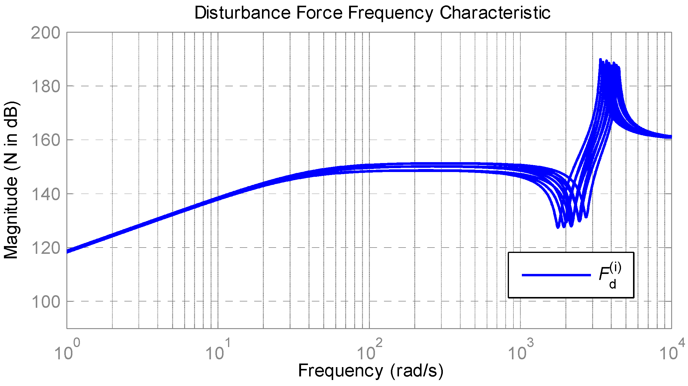According to the given parameters in Table 1 and computing the relative terms in Equation (6), the frequency characteristic curves of $F_{\mathrm{d}}$ for each equivalent linear model in $P_0(s)$ are acquired and are shown in Figure 5. As seen from Figure 5, the disturbance force $F_{\mathrm{d}}$ has differential characteristics at low frequencies and large magnitude (in dB).The magnitude of $F_{\mathrm{d}}$ rises with the slope of +20 dB as the frequency increases at low frequencies, tend to be saturated and stable in the middle frequency band, and sharply rise in high frequency region. In practice, the frequency of the position interference will not be high. Meanwhile, at low frequencies (less than 30 rad/s), the amount of $F_{\mathrm{d}}^{(\mathrm{i})}$ varies a little, about 1 dB for the models in $P_0(s)$, which means model perturbation has a small effect on the disturbance force of our interest.

Despite this disturbance force $F_{\mathrm{d}}$ is helpful when the direction of ${\dot{x}}_{\mathrm{M}}$ and $F_{\mathrm{L}}$ is opposite. However, generally, such a disturbance force will mostly increase the force error between the input and output, and it affects force-tracking accuracy. From the perspective of system control, this force error affects the closed-loop bandwidth of the loading system, and with the increase of the disturbance force, that bandwidth is seriously narrowed. It is difficult to achieve an ideal loading performance before this disturbance force has been effectively suppressed. Thus, the problem of disturbance force suppression should be solved firstly in the loading system; otherwise, the closed-loop bandwidth and the force-tracking accuracy cannot be guaranteed.

Generally, the motion amplitude and frequency of the booster are measurable and bounded; thus, the magnitude and frequency of $F_{\mathrm{d}}$ must be bounded and measurable. In a helicopter maneuvering system, the frequency of $x_{\mathrm{M}}$ is low, so $F_{\mathrm{d}}$ can be seen as a low-frequency disturbance.

3. Design of Hybrid Control Scheme

From the analysis above, strong disturbance and large parameter perturbation exist in the controlled plant. Despite that, other uncertainties such as friction and the gap in mechanical connection, which are unknown disturbances, also exist. Therefore, designing a robust control method for the controlled plant is needed.

Since robust control relates the amount of feedback at each frequency to the amount of uncertainty in the plant dynamics, the equivalent linear method forces the magnitude of the loop transmission to be unnecessarily large in the low-frequency range. If we take the robust approach directly, the result is an over-designed and conservative control system. Because it uses much more feedback gain than is actually required to solve the robust control problem, it does not even satisfy the performance requirements of the system. Thus, in order to effectively solve the control and synthesis for a loading system with large perturbation and strong motion disturbance, a hybrid control scheme is presented.

3.1. Constant Feed-Forward Compensator

As seen from Figure 3 and Figure 5, $F_{\mathrm{d}}$ is a measureable and bounded disturbance with large magnitude. From the perspective of control, using the conventional feed-forward control can suppress this disturbance, because the feed-forward control can compensate for the effect of this disturbance on system output before adverse effects. If the feed-forward regulator compensates the disturbance just right, the controlled variable will not produce deviation.

A control strategy based on the structure invariance principle is the most traditional one to compensate for this disturbance force because it does not change the structure of the closed loop, and it can be realized by software easily. According to the structure invariance principle, if we choose the velocity ${\dot{x}}_{\mathrm{M}}$ as the input (the observed motion disturbance) of the compensator and make

$$U_c(s)=G_{\mathrm{com}}(s){\dot{X}}_{\mathrm{M}}(s)=\frac{N_{\mathrm{D}}(s)}{N_{\mathrm{U}}(0)G_{\mathrm{v}}(s)}{\dot{X}}_{\mathrm{M}}(s)$$

(10)

the disturbance force $F_{\mathrm{d}}$ caused by ${\dot{x}}_{\mathrm{M}}$ will be canceled, and that means the extraneous force is suppressed completely. However, the robustness of this compensation is bad for system nonlinearity and time-varying parameters. In general, the velocity of the booster cannot be measured directly, and the rapidity and accuracy of the velocity obtained by the differential method or velocity estimation seriously affect the restraining ability. Moreover, $G_{\mathrm{com}}(s)$ is a non-proper transfer function, and it is difficult in physical implementation.

In this case, the frequency of ${\dot{x}}_{\mathrm{M}}$ is less than 3 Hz, and then $G_{\mathrm{v}}(s)$ can be approximately equal to $G_{\mathrm{v}}(0)$. It is well known that most of the disturbance force is related to the velocity of the motion disturbance in the low-frequency range. Then, a compensation term can be determined when ignoring the high-order factors in $N_{\mathrm{D}}(s)$ to eliminate the main part of the disturbance force as follows

$$G_{\mathrm{com}}(s)=\frac{N_{\mathrm{D}}(0)}{N_{\mathrm{U}}(0)G_{\mathrm{v}}(0)}$$

(11)

There are time-varying parameters in $N_{\mathrm{D}}(0)$ and $N_{\mathrm{U}}(0)$, and we take their middle values to obtain the constant compensation term $G_{\mathrm{com}}(0)=0.0486$.

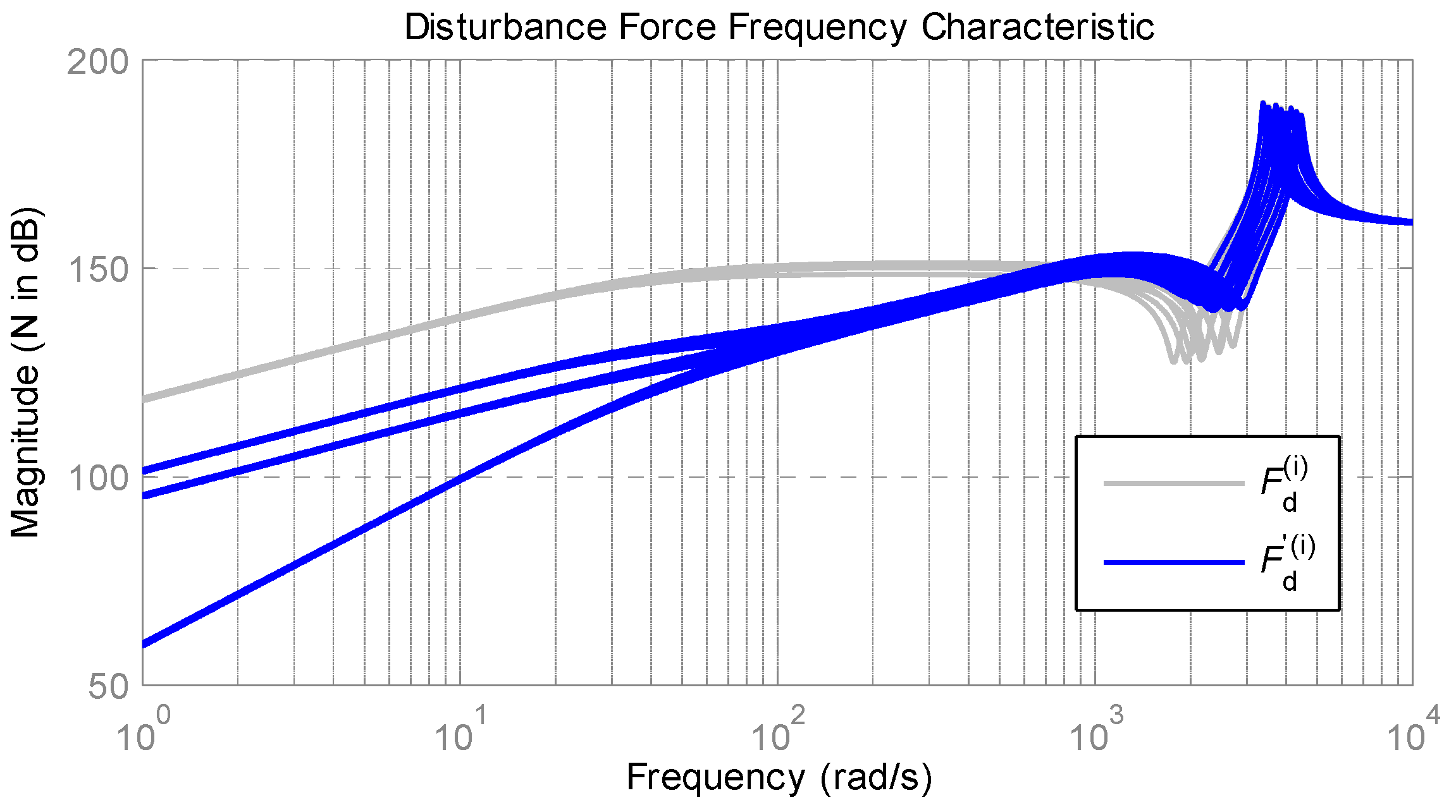
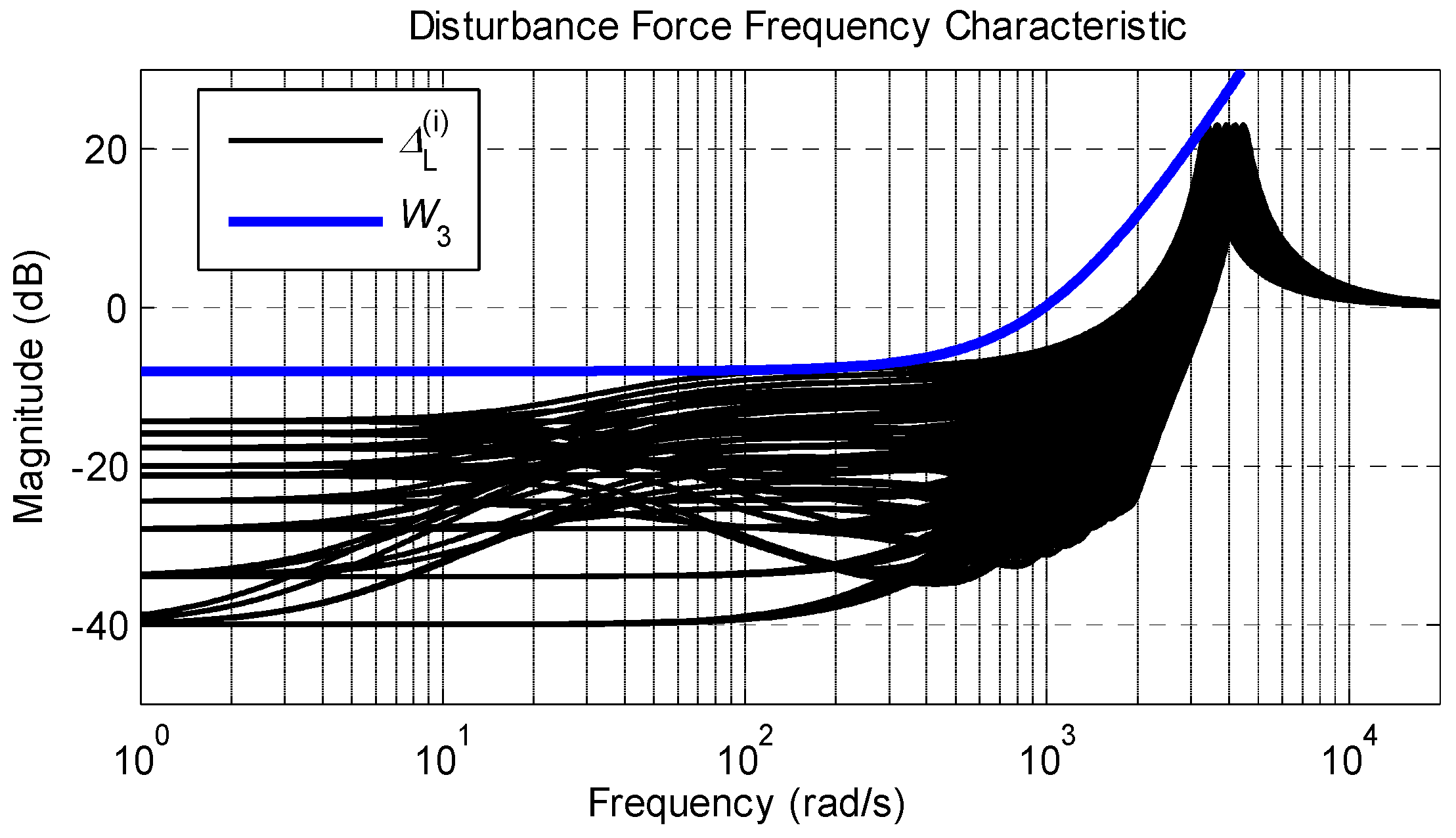
The characteristics of the disturbance force of models in $P_0(s)$, which are compensated by the constant compensator, are depicted in Figure 6. The velocity ${\dot{x}}_{\mathrm{M}}$ is acquired by the direct differential method. In Figure 6, $F_{\mathrm{d}}^{\prime (\mathrm{i})}$ represents the remaining disturbance force after compensation, and $F_{\mathrm{d}}^{(\mathrm{i})}$ represents the original disturbance force.

Although the restraining effect on the disturbance force of models in $P_0(s)$ differs within the concerned frequency range, the constant compensator at least attenuates the disturbance force 16 dB in magnitude; thus, at least 84% of the disturbance force is eliminated. However, the feed-forward compensator is sensitive to phase and the accuracy of the velocity signal. The restraining effect will degrade because it is difficult to get an ideal velocity signal in practical implementation. Therefore, the remaining extraneous force, after being compensated, will not be small enough, it will still affect the force-tracking performance, and it is necessary to restrain the remaining extraneous force further.

3.2. DOB-based Compensator

The remaining extraneous force, after been compensated by the constant velocity compensation, becomes an immeasurable disturbance with relatively small magnitude. From the perspective of control, the immeasurable disturbance can be compensated by an observer.

If controllers of the loading system are designed based on a double-loop cascade composition control strategy, two problems of disturbance rejection (including the remaining extraneous force) and force tracking can be solved separately. The inner loop controller is utilized to eliminate the remaining extraneous force and other disturbances, enhance system robustness, and make the actual plant behave as a nominal model approximately within certain operating bandwidth. The nominal model–based outer loop controller is used to realize the desired force-tracking performance. It is more reasonable to estimate the disturbance on the control channel than to estimate the disturbance itself because we can use the control input to improve the disturbance rejection performance. 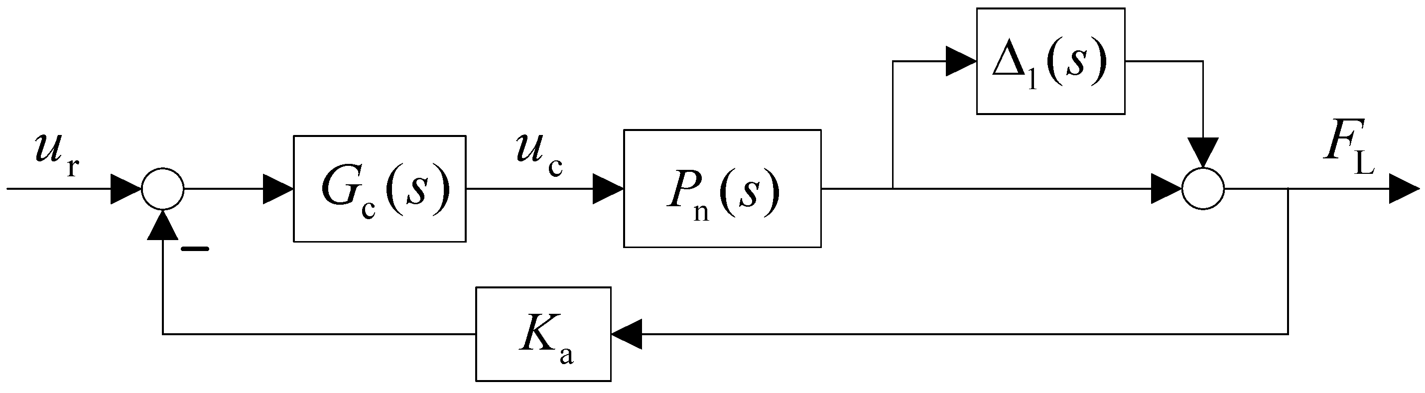Then the disturbance observer (DOB) method is introduced in Figure 7, where symbol $d_0$ represents the equivalent disturbance caused by un-modeled dynamics and unknown disturbances including friction.

The uncertainty of the system can be treated as a multiplicative perturbation of the nominal system, and it is given as

$$P(s)=P_{\mathrm{n}}(s)(1+{\Delta }_{\mathrm{L}}(s))$$

(12)

where ${\Delta }_{\mathrm{L}}$ is an allowable multiplicative uncertainty.

The DOB estimates a lumped disturbance, which includes the effects due to model uncertainties as well as the external disturbances, from the difference between the input-output relation of an actual plant $P(s)$ and its nominal model $P_n(s)$. The amount of the equivalent disturbance $d_0$ is estimated through the inverse nominal model $P_n^{-1}(s)$, and then the equivalent compensation is introduced into the control through a low-pass filter $Q(s)$, i.e., the cancellation input $u_{\mathrm{do}}$ is fed back into the control input, and thus a complete restraining of the equivalent disturbance is achieved.

Defining $d=(u_{\mathrm{vc}}+d_0)P-F_{\mathrm{d}}$, the transfer functions from each relevant input to output $F_{\mathrm{L}}$ can be written as

$$G_{F_{\mathrm{L}}{u}_{\mathrm{c}}}=\frac{F_{\mathrm{L}}}{u_{\mathrm{c}}}=\frac{P{P}_{\mathrm{n}}}{Q(P-P_{\mathrm{n}})+P_{\mathrm{n}}}$$

(13)

$$G_{F_{\mathrm{L}}d}=\frac{F_{\mathrm{L}}}{d}=\frac{P_{\mathrm{n}}(1-Q)}{Q(P-P_{\mathrm{n}})+P_{\mathrm{n}}}$$

(14)

$$G_{F_{\mathrm{L}}{\dot{x}}_{\mathrm{M}}}=\frac{F_{\mathrm{L}}}{{\dot{x}}_{\mathrm{M}}}=\frac{(G_{\mathrm{com}}(0)P-G_{\mathrm{d}})P_{\mathrm{n}}(1-Q)}{Q(P-P_{\mathrm{n}})+P_{\mathrm{n}}}$$

(15)

$$F_{\mathrm{L}}=G_{F_{\mathrm{L}}{u}_{\mathrm{c}}}{u}_{\mathrm{c}}+G_{F_{\mathrm{L}}d}d$$

(16)

In Equation (15), if $Q(s)\approx 1$ in the low-frequency range $[0,2]$ (Hz), the output from ${\dot{x}}_{\mathrm{M}}$ to $F_{\mathrm{L}}$ approximately equals zero, which means the disturbance force is well suppressed.

It is noticed that there is the same multiplicative factor $1-Q(s)$ from $d$ and ${\dot{x}}_{\mathrm{M}}$ to the output force $F_{\mathrm{L}}$, which means that the disturbance force can be regarded as the output resulting from the external disturbances. So the disturbance force can be regarded as a low-frequency disturbance.

The sensitivity function $S_{\mathrm{DOB}}$ and the complementary sensitivity function $T_{\mathrm{DOB}}$ of the DOB loop are derived as

$$\{\begin{array}{l}{S}_{\mathrm{DOB}}=\frac{1-Q(s)}{1+Q(s){\Delta }_{\mathrm{L}}(s)}\\ T_{\mathrm{DOB}}=\frac{(1+{\Delta }_{\mathrm{L}}(s))Q(s)}{1+Q(s){\Delta }_{\mathrm{L}}(s)}\end{array}$$

(17)

From the above analysis, the design of the DOB in our hybrid suppression scheme coincides with the design of the general DOB. When $Q(s)$ is designed, its cut-off frequency must be higher than the frequency of the disturbance force. At the same time, the frequency responses of sensitivity functions with the DOB should below enough to ensure sufficient disturbance attenuation besides the constraints of the traditional DOB, because the plant uncertainty is negligible in the low-frequency region.

It is well known that the key of the DOB design is the design of $Q(s)$. Once the nominal model is chosen, the upper bound of the uncertainty against the nominal model is confirmed, and the upper limitation bandwidth of $Q(s)$ is decided. The tracking performance is enhanced by increasing the order and the bandwidth of $Q(s)$, but the excessive order and bandwidth of $Q(s)$ can lead to resultant destruction of the stability condition due to plant uncertainty in the high-frequency region. The design of $Q(s)$ is a trade-off between disturbance suppression and robustness. If $Q(s)$ is designed appropriately, the disturbance observer not only suppresses the rest disturbance, but also fulfills robustness.

Apparently, solving the model mismatch in an overall frequency band through the DOB loop compensator is unrealistic. Therefore, the DOB-based inner loop compensator is designed mainly to solve the suppression problem of the extraneous force, other low-frequency external interference and model mismatch at low frequencies, as well as taking some proper consideration of the system model mismatch at middle and high frequencies. The model mismatch in the middle- and high-frequency range can be considered in the outer loop control.

3.3. Robust Performance Controller

Equation (13) can be transformed into

$$G_{F_{\mathrm{L}}{u}_{\mathrm{c}}}(s)=P_{\mathrm{n}}(s)\left[1+\frac{1-Q(s)}{1+Q(s){\Delta }_{\mathrm{L}}(s)}{\Delta }_{\mathrm{L}}(s)\right]$$

(18)

The controlled plant is changed because of the feedback of the DOB loop. However, from the relationship between $u_{\mathrm{c}}$ to $F_{\mathrm{L}}$ in Equation (18), it is obvious that the outer loop controlled plant is still a model with multiplicative perturbation, and its structure can be equivalent to a virtual controlled plant $P_{\mathrm{n}}(s)(1+{\Delta }_1)$, where $P_{\mathrm{n}}(s)$ is the nominal model and ${\Delta }_1=\frac{1-Q(s)}{1+Q(s){\Delta }_{\mathrm{L}}(s)}{\Delta }_{\mathrm{L}}(s)$.

In our loading system with dynamic load superimposed on static load, the force signal to be tracked is in the sinusoidal form or the form of sine superposition offset; a feedback controller is therefore adequate for the outer loop. Therefore, a robust feedback controller based on the H∞ theory is designed, and the structure of the outer loop is shown in Figure 8.

If the $Q(s)$ is appropriately designed, the design specifications of the outer loop feedback controller may not consider the disturbance attenuation requirement. Therefore, the outer loop controller $G_{\mathrm{c}}(s)$ may not include an integrator. From the small gain theorem, the sufficient and necessary condition for the stability and robustness of $G_{\mathrm{c}}(s)$ is

$$\Vert {\Delta }_1{T}_{\mathrm{ou}}\Vert <1\text{ and }{T}_{\mathrm{ou}}=\frac{P_{\mathrm{n}}{G}_{\mathrm{c}}}{1+P_{\mathrm{n}}{G}_{\mathrm{c}}}$$

(19)

3.4. Hybrid Control Scheme

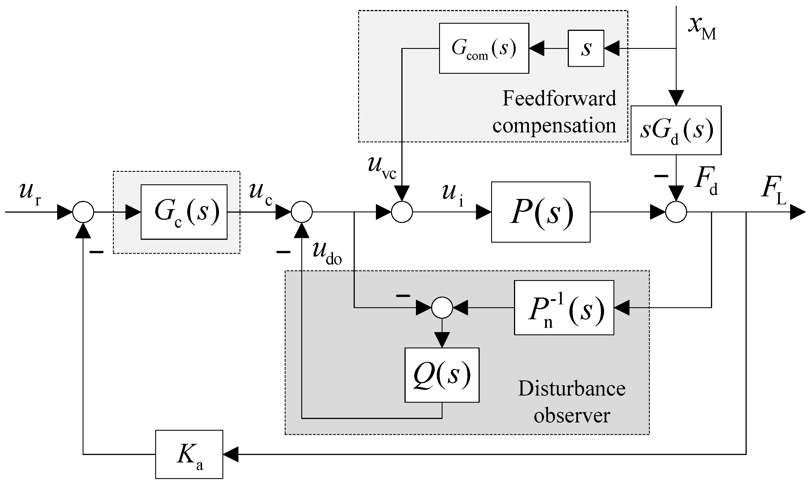
From the design above, the hybrid control scheme is obtained and its schematic diagram is shown in Figure 9.

The hybrid control scheme consists of a constant velocity feed-forward compensator and double-loop cascade composition control strategy. The constant velocity compensator generates compensation input $u_{\mathrm{vc}}$ to eliminate most of the extraneous force. The disturbance observer–based inner loop compensator generates compensation input $u_{\mathrm{do}}$ to restrain disturbances besides the remaining extraneous force, and makes the actual plant tracking approximately a nominal model in a certain frequency range. In addition, the robust outer loop controller generates $u_{\mathrm{c}}$ to achieve the desired force-tracking accuracy, and guarantees system robustness in the high-frequency region.

Thus, the control law of the hybrid control scheme is obtained. The control input $u_{\mathrm{i}}$ consists of three parts with different functions as follows

$$u_{\mathrm{i}}=u_{\mathrm{c}}+u_{\mathrm{vc}}-u_{\mathrm{do}}$$

(20)

Under the same model perturbation, the tracking performance of the robust controller that can be achieved is limited. The direct robust method might achieve the same disturbance suppression ability (in dB) with the hybrid control scheme. However, the tracking error of the direct robust method is far greater than that of the hybrid control scheme, and therefore the tracking performance of the direct robust method is lower than that of the hybrid control scheme.

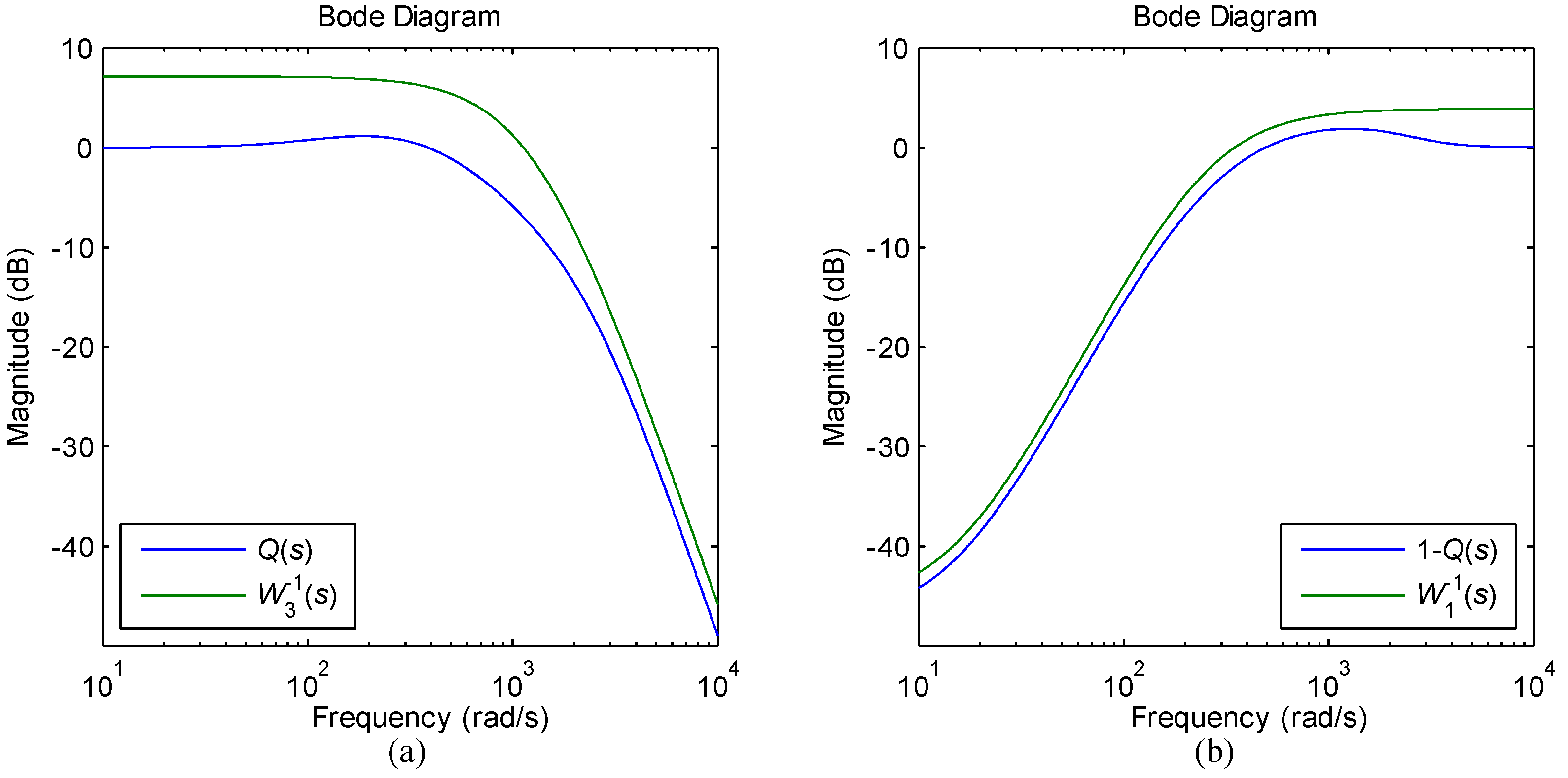
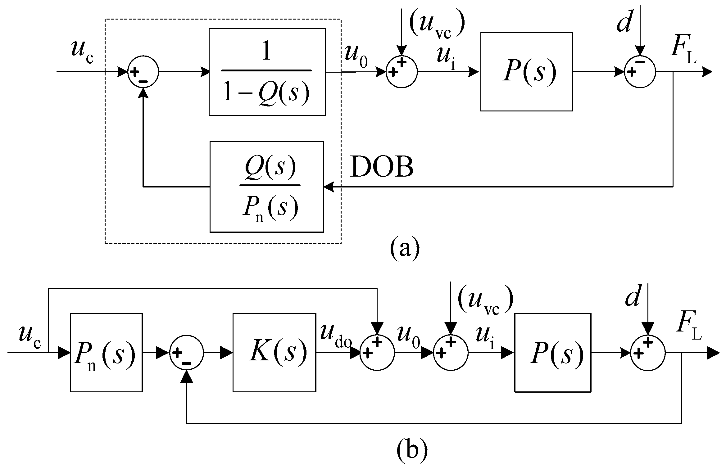
3.5. Design Method of Q(s)

The design and optimization of $Q(s)$ in Figure 7 is not easy when the requirements of performance and robustness must be considered together, especially when there are some performance demands. A systematic method in dealing with this issue was proposed in [32]. The block diagram transformation for Figure 7 yields Figure 10a. In order to use robust control theory, we take

$$Q(s)=\frac{P_{\mathrm{n}}(s)K(s)}{1+P_{\mathrm{n}}(s)K(s)}$$

(21)

where the internal-loop compensator $K(s)$ is stable. Then the structure of the hybrid suppression scheme can be transformed equivalently to a structure in Figure 10b. In this way, the design of $Q(s)$ can be transformed to the design of $K(s)$.

In Figure 10, $K(s)$ is the robust internal-loop feedback controller. If $K(s)$ is designed for the nominal model $P_{\mathrm{n}}(s)$ in order to satisfy a given performance and robustness criterion, the optimal $Q(s)$ of the DOB can be systematically designed by the optimal method under the given specific conditions, because the transfer function of the unity feedback system with $P_{\mathrm{n}}(s)$ and $K(s)$ can determine $Q(s)$ in Equation (21).

The H∞ mixed sensitivity method is utilized to derive the optimal robust internal loop compensator $K(s)$, and then the optimal $Q(s)$ can be derived by Equation (21). The sensitivity function $S_{\mathrm{Q}}$ and the complementary sensitivity function $T_{\mathrm{Q}}$ of $Q(s)$ are obtained from Equation (22), respectively

$$S_{\mathrm{Q}}=\frac{1}{1+P_{\mathrm{n}}(s)K(s)},T_{\mathrm{Q}}=\frac{P_{\mathrm{n}}(s)K(s)}{1+P_{\mathrm{n}}(s)K(s)}$$

(22)

Apparently, $S_{\mathrm{Q}}=1-Q$ and $T_{\mathrm{Q}}=Q$. Then the H∞ mixed sensitivity problem can be described as solving $K(s)$ to meet the minimum H∞ norm

$$\underset{K_{stabilizing}}{\min }{\Vert \begin{array}{c}{W}_1(1-Q)\\ W_{3}Q\end{array}\Vert }_{\infty }<1$$

(23)

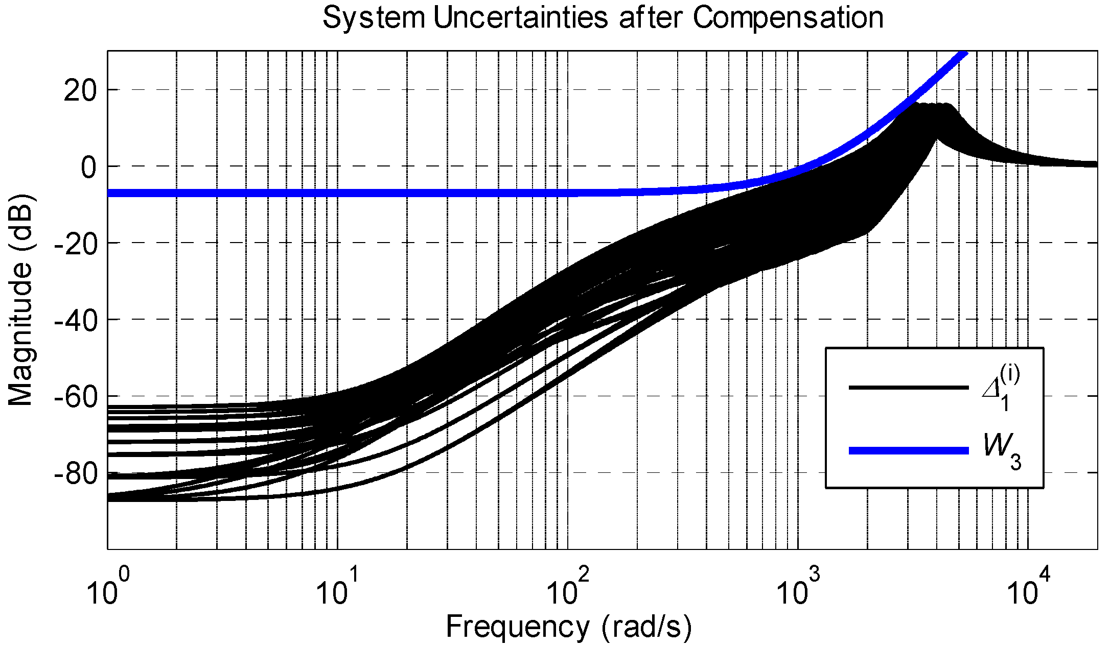
Then, this provides a simple way to do trade-offs. In light of this, the characteristics of $Q(s)$ can be planned through the design of weighting functions, and they make it easy to consider the middle and high frequency part of $Q(s)$, which can guarantee the robustness, but the model error is amplified in some frequency bands, which restricts the closed-loop bandwidth.

4. System Design

4.1. Nominal Model

One nominal model is needed in the presented hybrid control scheme, because both $Q(s)$ and $K(s)$ are designed based upon it. From the analysis above, the difference between the nominal model and the actual plant, that is the uncertainty of the nominal model, determines the maximum allowable bandwidth, and therefore restricts the system performance.

However, it can get a better result of design if the nominal model approximates the actual plant as far as possible. In our system, the derived equivalent linear models $P_0(s)$ with parameter variation are fifth-order models. The inverse of the fifth-order model will be extremely sensitive to high-frequency noise. Thus, a low-order model is appropriate; moreover, the low-order nominal model makes the design of the DOB simple.

From Equation (9) and Figure 4, it is observed that system characteristics are mainly determined by the inertial frequency ${\mathsf{\omega }}_{\mathrm{L}}$ of the hydraulic actuator, the second-order resonance frequency ${\mathsf{\omega }}_{\mathrm{v}}$ of the servo valve, and the gain $K_{\mathrm{op}}$. According to the idea of a dominant pole, if we take the middle value of ${\mathsf{\omega }}_{\mathrm{L}}$ and $K_{\mathrm{op}}$ as nominal values and treat the second-order oscillation term of the hydraulic actuator as the perturbation, then a third-order nominal model $P_n(s)$ is obtained as

$$P_n(s)=\frac{424908834}{(s+38.82)(s^2+1759s+1579000)}$$

(24)

The uncertainty ${\Delta }_{\mathrm{L}}$ of the system, which is treated as a multiplicative perturbation can be calculated by

$${\Delta }_{\mathrm{L}}(s)=P(s)/P_{\mathrm{n}}(s)-1$$

(25)

4.2. Design of Q(s)

In the design of $Q(s)$, the weighting function $W_3(s)$ represents the upper limitation of the system uncertainty, and it can be designed according to the model uncertainty ${\Delta }_{\mathrm{L}}$. In Figure 11, the black lines represent the possible multiplicative perturbation ${\Delta }_{\mathrm{L}}^{(\mathrm{i})}$ of the models in $P_0(s)$ against the nominal model $P_{\mathrm{n}}(s)$. In order to cover all the possible uncertainties ${\Delta }_{\mathrm{L}}^{(\mathrm{i})}$, $W_3(s)$, the blue line in Figure 11, is obtained as

$$W_3(s)=1.914\times {10}^{-10}{(s+1320)}^3$$

(26)

The weighting $W_1(s)$ is the spectrum characteristics of the interference. The weighting reciprocal $W_1^{-1}(s)$ determines the ability of disturbance suppression. In order to suppress 95% of the equivalent disturbance below 3 Hz, $W_1(s)$ can be chosen as

$$W_1(s)=\frac{0.64{(s+262.5)}^2}{{(s+15)}^2}$$

(27)

By solving the mixed sensitivity problem described in Equation (23) with MATLAB Control System Toolbox (MathWork, New York, NY, USA, 2010) and Robust Control Toolbox (MathWork, New York, NY, USA, 2010), $K(s)$ is obtained. After being computed by Equation (21), $Q(s)$ can be determined as

$$Q(s)=\frac{1.752\times {10}^{15}s+2.137\times {10}^{17}}{s^5+485255s^4+2.293\times {10}^9{s}^3+4.153\times {10}^{12}{s}^2+1.875\times {10}^{15}s+2.147\times {10}^{17}}$$

(28)

Figure 12a,b display the magnitude frequency response curves of $Q(s)$, $W_1^{-1}(s)$, $1-Q(s)$ and $W_3^{-1}(s)$, respectively. Obviously, the robust stability condition and the interference suppression requirement of the DOB system are both satisfied.

As seen from Figure 12a, the maximum frequency bandwidth of $Q(s)$ is directly limited by the weighting function $W_3(s)$, and thus it is very important to determine one appropriate $W_3(s)$.

Meanwhile, $1-Q(s)$ determines the ability of interference suppression. From Figure 12b, the remaining extraneous force will be attenuated to −42 dB (decreased by 98.7%) at least; that is, combined with the constant velocity compensator, the extraneous force will be eliminated almost completely. Other low-frequency disturbance will also be suppressed effectively. Then, the disturbance will have little effect on the force-tracking error.

4.3. H∞ Controller

After $Q(s)$ is designed, the virtual plant of the outer loop is made certain, and then ${\Delta }_1$ can be calculated, as is shown in Figure 13, in which $W_3(s)$ is also drawn for comparison. In Figure 13, the black lines represent the possible multiplicative perturbation ${\Delta }_1^{(\mathrm{i})}$ of the models in $P_0(s)$ against the nominal model $P_{\mathrm{n}}(s)$, which is compensated by the DOB. Compared with ${\Delta }_{\mathrm{L}}$, the uncertainty is restrained significantly in the low-frequency region, while in the middle- and high-frequency regions, the uncertainty enlarges some, but it is still below $W_3(s)$. This means the allowable bandwidth of the system changes little after being compensated by the DOB, while the system perturbation decreases greatly in the low-frequency region. The function $W_3(s)$ can be a candidate weighting function to describe the uncertainty of the outer loop.

The H∞ mixed sensitivity method is used to derive the performance controller $G_{\mathrm{c}}(s)$. The sensitivity function $S_{\mathrm{c}}$ and the complementary sensitivity function $T_{\mathrm{C}}$ of the outer loop are deduced according to the definition of robust control theory as

$$S_{\mathrm{C}}=\frac{1}{1+P_{\mathrm{n}}(s)G_{\mathrm{c}}(s)},T_{\mathrm{C}}=\frac{P_{\mathrm{n}}(s)G_{\mathrm{c}}(s)}{1+P_{\mathrm{n}}(s)G_{\mathrm{c}}(s)}$$

(29)

The performance weighting function $W_{1\mathrm{o}}(s)$ of the outer loop is set as

$$W_{1\mathrm{o}}(s)=\frac{3.017\mathrm{s}+17500}{33.33\mathrm{s}+1}$$

(30)

Set $W_{3\mathrm{o}}(s)=W_3(s)$, $W_{2\mathrm{o}}(s)=0.00001$, and then solving the standard H∞ mixed sensitivity problem, $G_{\mathrm{c}}(s)$ is obtained as

$$G_{\mathrm{c}}(s)=\frac{4809662.1287(s+38.82)(s^2+1759s+1579000)}{(s+426300)(s+0.03)(s^2+4509s+7399000)}$$

(31)

The closed-loop characteristic curve of the nominal plant is displayed in Figure 14.

5. Simulation Experiment

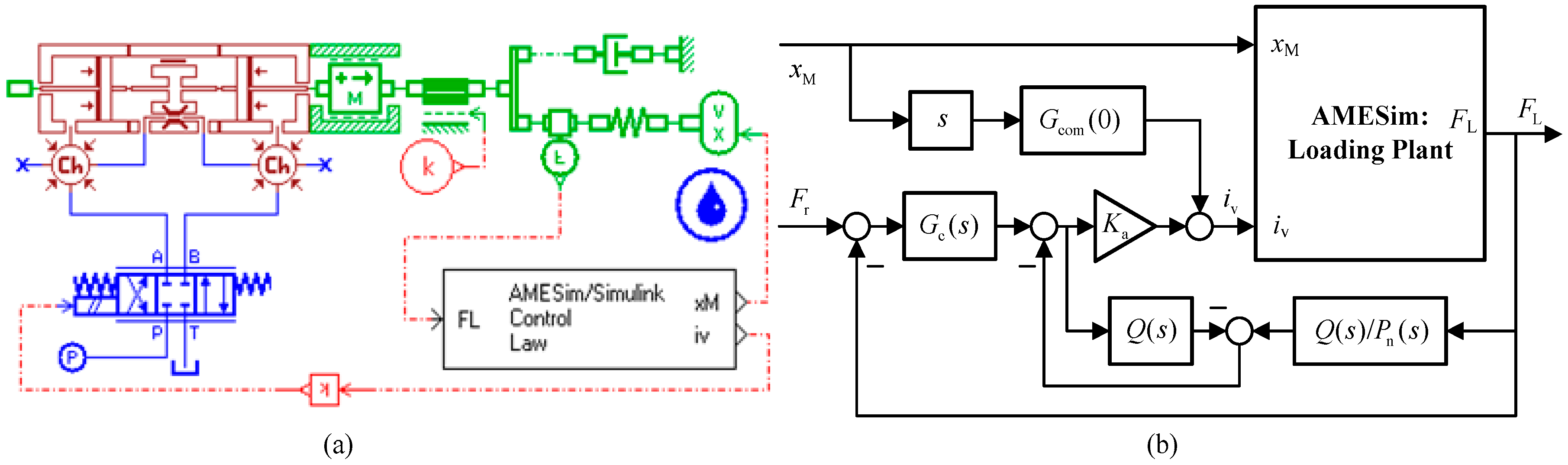
In the above sections, the outer loop controller and the disturbance compensator have been designed based on the established linear mathematical model with perturbations. The influence of some factors has been neglected, and part of the system nonlinearity has been treated by equivalent linearization. In order to validate the effectiveness of the designed hybrid controller, a simulation model that is close to the practical situation is needed. So, in the simulation experiment section, the model of the loading system is built in AMESim (LMS Imagine, Leuven, Belgium, 2010), as depicted in Figure 15a; it contains the nonlinear characteristics of the load flowrate of the servo valve and the un-modeled dynamics, and it is closer to the actual plant than the linear model. The developed algorithm is conducted in MATLAB/Simulink (MathWork, New York, NY, USA, 2010). Through co-simulation using AMESim and MATLAB/Simulink as shown in Figure 15b, the performance of the designed hybrid controller can be evaluated. The schematic diagrams of co-simulation are shown in Figure 15.

In Figure 15a, the gain block with a value of 1000 is used to convert the unit of the control current of the servo valve from amperes (A) in MATLAB to milliamperes (mA) in AMESim, and the gain for the signal output of the force sensor is set to −1 to make the output direction of the force sensor consistent with Equation (1).

In the AMESim model, besides the nonlinear dynamic characteristics of the servo valve, the following factors are considered: the supply pressure; the internal leakage, static friction, Coulomb friction and viscous friction of the loading cylinder; the equivalent mass of the load; and the oil bulk modulus. Parameters related to the loading cylinder are chosen according to the characteristics of the servo hydraulic cylinder in the industrial environment. A friction model with the Stribeck effect is designed. The used parameters in AMESim are listed in

Table 2. Parameters in AMESim.

Parameter	Value	Parameter	Value
Supply pressure $p_{\mathrm{s}}$	180–210 bar	Clearance on diameter	0.02 mm
Maximum flow rate	40 L/min	Coefficient of viscous friction	800 N/(m/s)
Rated pressure drop	70 bar	Maximum static force	150 N
Valve rated current	20 mA	Maximum Coulomb friction	100 N
Valve natural frequency	200 Hz	Force sensor stiffness	1 × 108 N/m
Valve damping ratio	0.7	Dead volume	40 cm3
Piston diameter	70 mm	Mass $m_{\mathrm{L}}$	8–12 kg
Rod diameter	42 mm	Oil modulus ${\mathsf{\beta }}_{\mathrm{e}}$	7000–11,000 bar
Full stroke	150 mm	Oil density	870 kg/m3

and are consistent with those in Table 1.

In the course of co-simulation, all experiments are performed under the typical operating condition, i.e., in the presence of motion disturbance, and some unified settings are made: (1) The motion disturbance input is set as $x_{\mathrm{M}}$ = 7sin14t (mm/s) unless otherwise stated to produce the largest motion disturbance. Its magnitude is higher than the maximum magnitude when the motion disturbance is at its maximum frequency. (2) The ${\dot{x}}_{\mathrm{M}}$ is acquired by the direct differential method. (3) The nominal values of the perturbed parameters $p_{\mathrm{s}}$, ${\mathsf{\beta }}_{\mathrm{e}}$, and $m_{\mathrm{L}}$ are 21, 900 MPa, and 10 kg, respectively. (4) The AMESim print interval is set as 0.0001 s.

5.1. Disturbance Suppression without Loading Force Command

As noted above, the ability of disturbance suppression of the loading system has a severe effect on the force-tracking performance. To verify the ability of disturbance suppression, the loading force command $F_{\mathrm{r}}$ is always set to zero in this section.

5.1.1. Suppression Performance

In the proposed hybrid control scheme, the extraneous force is gradually eliminated by the composite methods. Therefore, four kinds of experiments are successively made to verify their corresponding suppressing effects. All experiments are conducted under the conditions that the motion disturbance input is 7sin14t (mm/s), the force feedback loop is always closed and all perturbed parameters take their nominal values.

(1)

The original extraneous force is tested for comparison in the condition that the outer loop controller $G_{\mathrm{c}}(s)=1$ and without the constant compensation term and DOB inner loop compensator.

(2)

The suppression by using the constant compensator. In this case, there is no DOB inner loop compensator and the outer loop controller $G_{\mathrm{c}}(s)=1$.

(3)

The suppression by using the constant compensator combined with the DOB inner loop compensator. In this case, the outer loop controller $G_{\mathrm{c}}(s)=1$.

(4)

The suppression by using the designed hybrid controller.

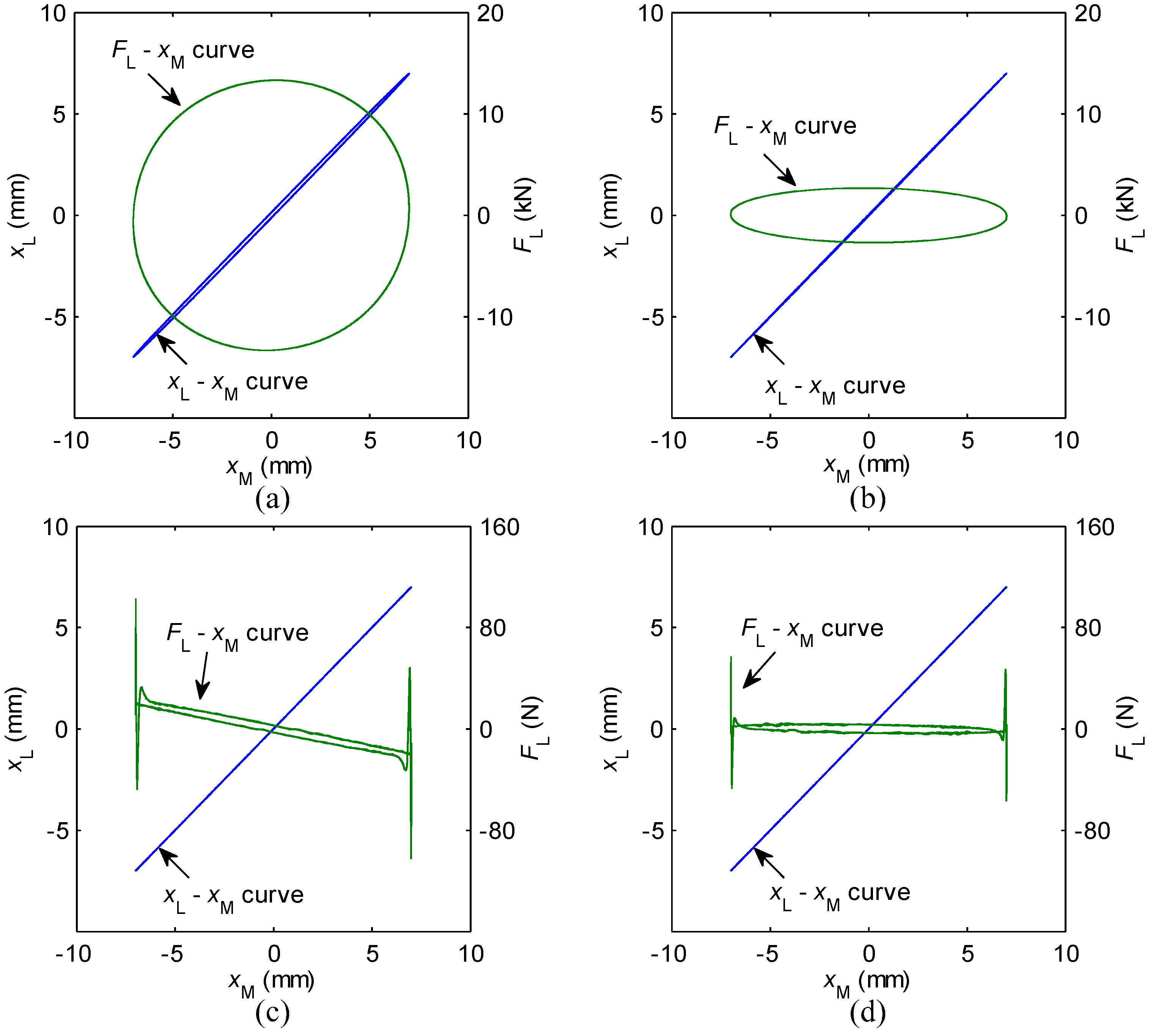
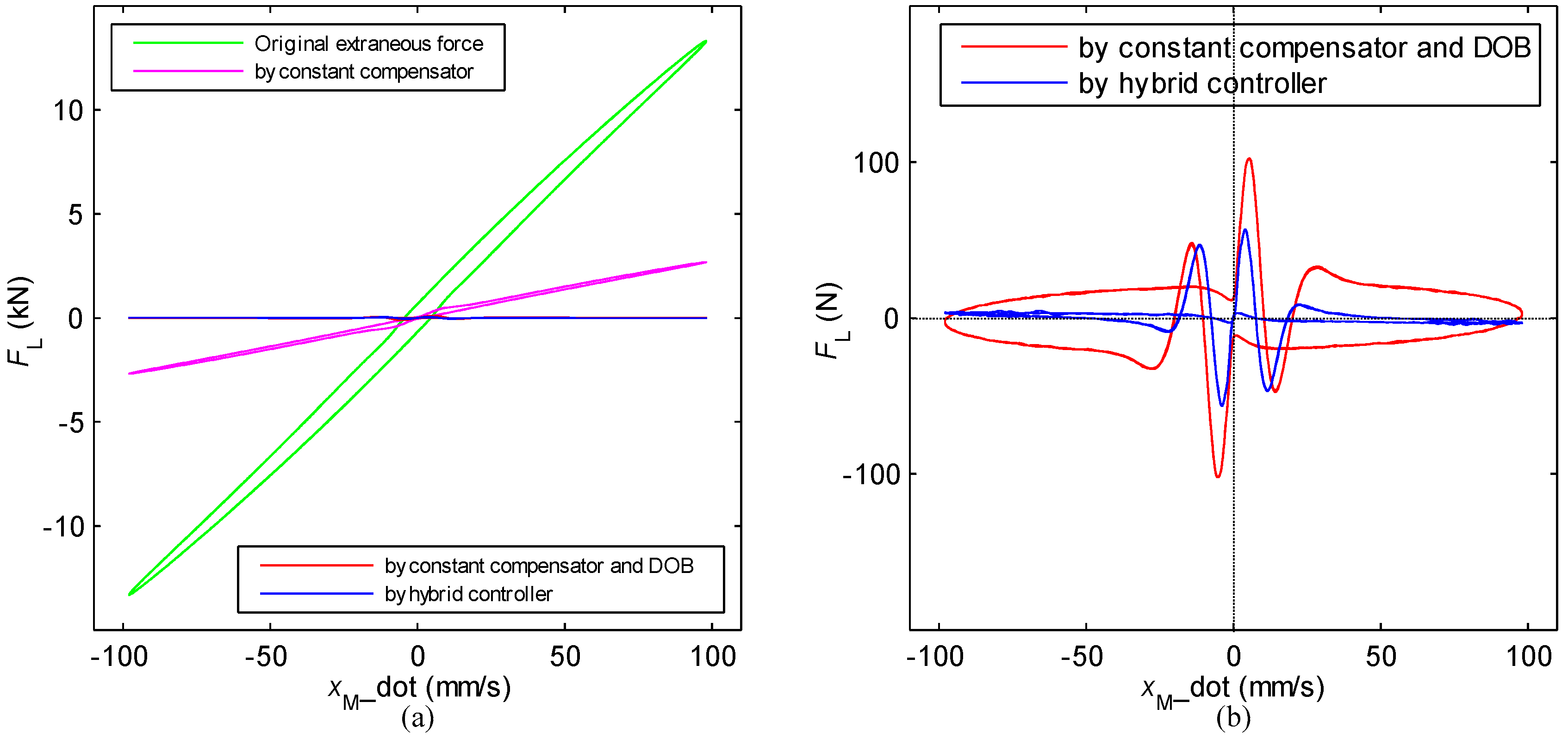
The experimental results are drawn in the form of a Lissajous curve, and are depicted in Figure 16 and Figure 17, because $x_{\mathrm{M}}$, $x_{\mathrm{L}}$ and $F_{\mathrm{L}}$ have the same frequency when the loading force command equals zero.

In Figure 16, the curves of $F_{\mathrm{L}}$ and $x_{\mathrm{L}}$ to $x_{\mathrm{M}}$ have a clear physical meaning, and they illustrate the formation of the output force which is defined by Equation (1). In this case, the output force is the extraneous force. The smaller the spacing in the middle region of the curve of $x_{\mathrm{L}}$ to $x_{\mathrm{M}}$, the smaller the extraneous force is. In Figure 17, the curve of $F_{\mathrm{L}}$ to ${\dot{x}}_{\mathrm{M}}$ illustrates the relationship between the disturbance velocity and the extraneous force, and provides the information about when and how the extraneous force gets its maximum value. This curve is useful for evaluating the suppressing effect on the extraneous force.

As seen from Figure 16 and Figure 17, the original extraneous force is very big (up to 13,310 N, in Figure 16a and Figure 17a). It is far beyond other disturbances in the loading system, and even more than some command loading forces. It is meaningful to suppress the extraneous force. After being compensated by the constant compensator, the extraneous force is decreased to 2688 N (decreased by 80%, in Figure 16b and Figure 17a). This result is very close to the analysis result about the suppressing ability of the constant compensator in Section 3.1 (decreased by 84%). By using the constant compensator combined with the DOB inner loop compensator, the extraneous force is further reduced to 102 N (decreased by 96.2% from 2688 N, in Figure 16c and Figure 17b). This result is close to our design in Section 4.2 where the designed Q-filter can attenuate the disturbance up to −42 dB (decreased by 98.7%). With the designed hybrid controller, the extraneous force is restrained to 57 N (decreased by 99.6% from the original extraneous force, in Figure 16d and Figure 17b). This implies that the proposed hybrid control scheme and controller are valid, and achieve excellent suppression of the disturbance force (less than 60 N) even with the largest motion disturbance.

Notice that in Figure 16c,d and Figure 17b, there are obvious burrs and peak values on the curves of $F_{\mathrm{L}}$ to $x_{\mathrm{M}}$ and $F_{\mathrm{L}}$ to ${\dot{x}}_{\mathrm{M}}$. The high burrs on the curve of $F_{\mathrm{L}}$ to $x_{\mathrm{M}}$ appear nearly at the maximum displacement, and the sharp peaks on the curve of $F_{\mathrm{L}}$ to ${\dot{x}}_{\mathrm{M}}$ occur around ${\dot{x}}_{\mathrm{M}}=0$. 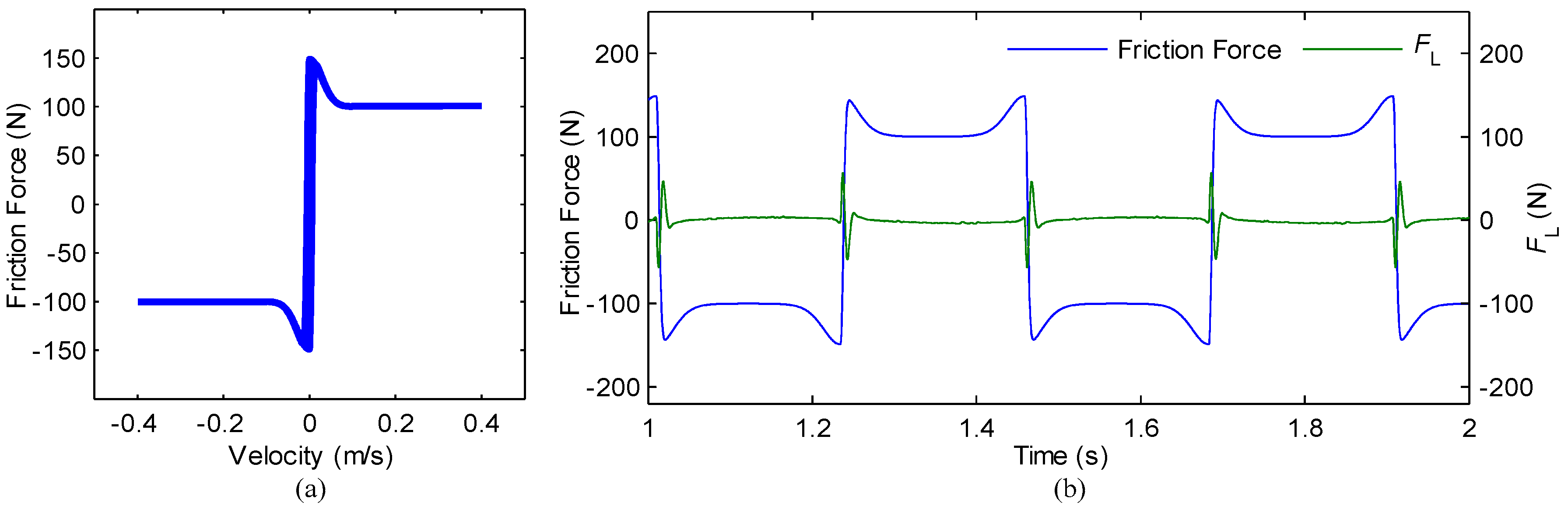This implies there is a relationship between the generation of sharp force disturbance and the changes in the direction of motion. From the characteristic of friction force versus velocity ${\dot{x}}_{\mathrm{L}}$ of the hydraulic cylinder, as depicted in Figure 18a, the friction force is changed sharply when the direction of ${\dot{x}}_{\mathrm{L}}$ changes. Moreover, from the corresponding graph of the friction force and $F_{\mathrm{L}}$ in the time domain, as depicted in Figure 18b, the start time of the peak of the force output is just corresponding to the time when the friction force is changing. Thus, this sharp force disturbance is mainly caused by the impact friction force of the hydraulic cylinder that is generated when the motion is reversing.

It can be verified that the curves of $F_{\mathrm{L}}$ to $x_{\mathrm{M}}$ and $F_{\mathrm{L}}$ to ${\dot{x}}_{\mathrm{M}}$ are close to ellipses in the absence of friction force. Without the impact of friction force, the maximum output force will be 20 N in Figure 16c and 5 N in Figure 16d, and that means the extraneous force resulting from the disturbance motion is successfully suppressed. Simultaneously, it is known from Figure 17b and Figure 18b that the designed hybrid controller has a certain restraining ability on friction force (reduced from 150 to 57 N), but the restraining effect is worse than that of the extraneous force. In order to verify our design of the hybrid controller, the assumed friction force is larger than the actual low-friction servo hydraulic cylinders. Therefore, in practical application, the impact of the friction force will be relatively small.

5.1.2. Robustness of Suppression

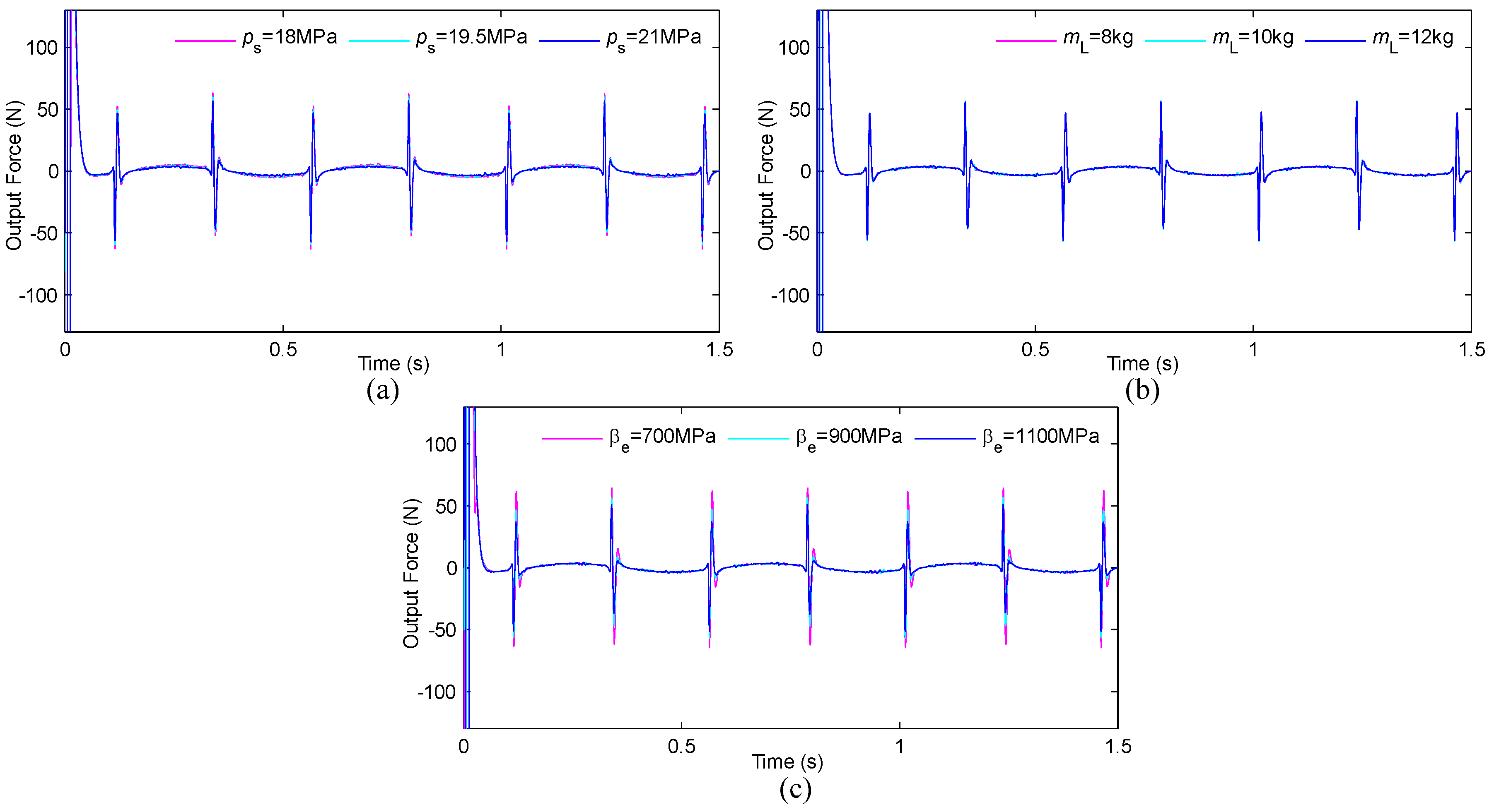
When designing the controllers, the perturbations of some system parameters have been taken into consideration. The designed hybrid controller achieves a good disturbance suppression performance with the nominal values of perturbation parameters. The influence of each perturbation parameter on the disturbance suppression is studied separately, meaning that when a parameter is perturbed, the other parameters are taking their nominal values. The experiments are carried out with the designed hybrid controller.

Figure 19a–c show the restraining results for different $p_{\mathrm{s}}$, ${\mathsf{\beta }}_{\mathrm{e}}$ and $m_{\mathrm{L}}$, respectively. It is observed that the perturbation of $p_{\mathrm{s}}$ and ${\mathsf{\beta }}_{\mathrm{e}}$ causes a very small increase in the maximum value of the output force (less than 5 N), while there is almost no effect for the perturbation of $m_{\mathrm{L}}$. It can also be known from Figure 19b that increasing fluid bulk modulus ${\mathsf{\beta }}_{\mathrm{e}}$ is beneficial to disturbance suppression.

Therefore, we can draw that the disturbance force, including the extraneous force and the friction force, is effectively suppressed by the proposed hybrid control scheme and controller, and it has considerable robustness within the perturbation range of our study.

5.2. Loading Force Tracking

5.2.1. Typical Loading Force Case

The command loading forces are applied to verify the tracking performance of the designed H∞ feedback controller, because the strong disturbance force has already been effectively restrained by the compensators.

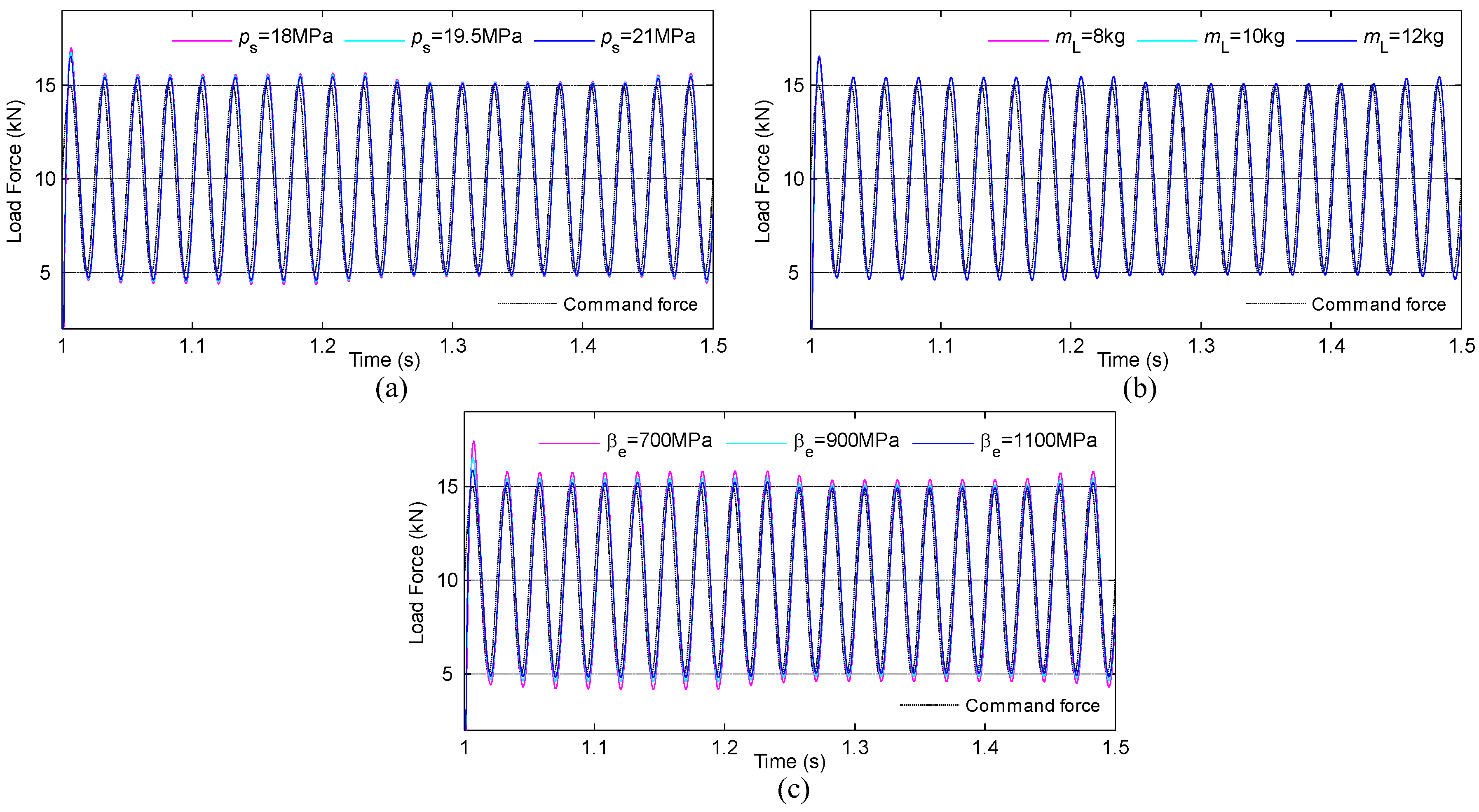
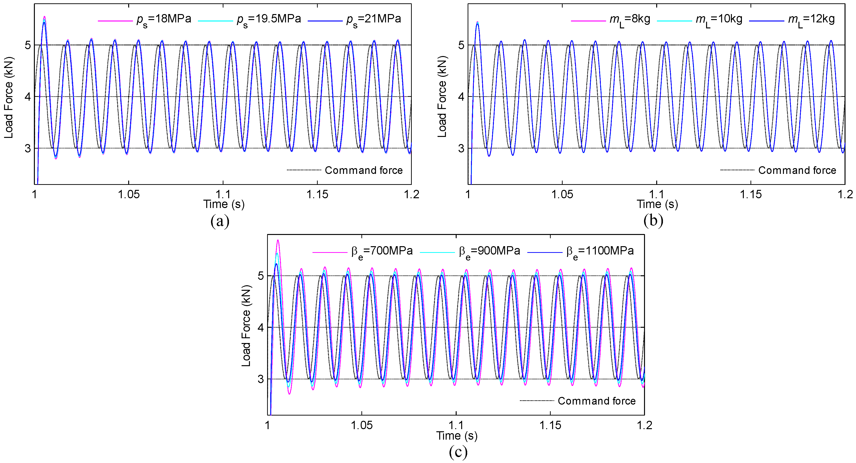
Two typical types of loading force spectrum are acted on the system. They are all in the form of dynamic load superimposed on a large static load, and they are different in amount and frequency of dynamic load. One is $10+5\sin 80\mathsf{\pi }t$ (kN), and the other is $4+\sin 160\mathsf{\pi }t$ (kN). During the experiment, the motion disturbance is always exerted on the loading system. At the same time, the influence on force tracking by the perturbation parameters is also taken into account. For different command loading forces, the curves of $F_{\mathrm{L}}$ and $x_{\mathrm{L}}$ to $x_{\mathrm{M}}$ are not regular because their frequencies are not the same. Therefore, we analyze the loading performance in the time domain. The results of two kinds of loading forces are shown in Figure 20 and Figure 21, respectively.

From the experimental results, there are some relatively consistent results. The perturbation of $m_{\mathrm{L}}$ has almost no effect on the load output. The perturbation of $p_{\mathrm{s}}$ has a small effect on the load output, and the best tracking performance is achieved at the maximum supply pressure. The perturbation of ${\mathsf{\beta }}_{\mathrm{e}}$ has an obvious effect on the load output, and when ${\mathsf{\beta }}_{\mathrm{e}}$ equals 700 MPa the maximum magnitude error to the loading force command reaches 5.2% in Figure 20a and 3% in Figure 21a, respectively. This is because larger $p_{\mathrm{s}}$ and ${\mathsf{\beta }}_{\mathrm{e}}$ increases the open loop bandwidth of the system, and thus the error between the physical plant and the nominal model will be reduced, and that means the H∞ controller can use more gain in tracking. It can be verified that if the ${\mathsf{\beta }}_{\mathrm{e}}$ is set to 1100 MPa, the output error will be less than 2% for all the above experiments, and this can be easily implemented in engineering. So, the tracking performance of the designed H∞ controller can be guaranteed in the range of allowable perturbations.

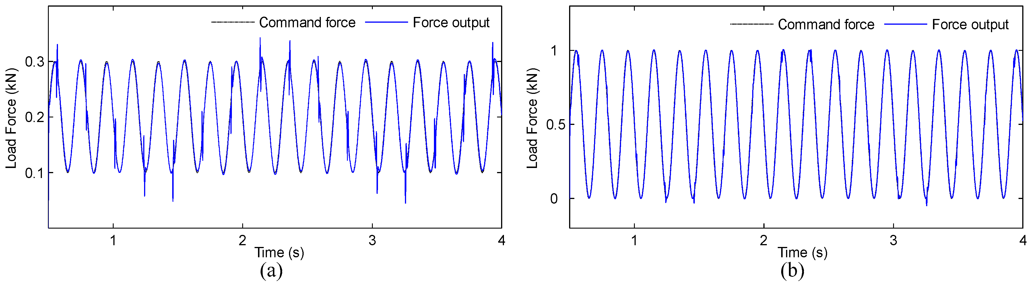
5.2.2. Small Command Loading Force Case

Our typical loading force spectrums are relatively large, and are much larger than the friction force. The effect of the friction force on the output force is not easily observed. Then, we performed the experiments with a small command loading force of $200+100\sin 10\mathsf{\pi }t$ (N) and a slightly larger force with the same frequency of $500+500\sin 10\mathsf{\pi }t$ (N). During the experiment, all perturbation parameters take their nominal values and the motion disturbance always exerts on them.

From the results in Figure 22a,b, friction has a certain effect on the output of a small command loading force, but the output shape is still maintained. In addition, that effect is not obvious for a slightly larger command loading force.

5.2.3. Comparative Results of Different Outer Loop Controllers

There are two purposes for the design of the DOB inner loop compensator. One is to suppress the disturbance including the extraneous force and friction. The other is to compensate the model mismatch between the nominal model and the controlled plant, and to make the controlled plant behave like the nominal model in a certain frequency range. Through the above analysis, the DOB compensated plant can be treated as $P_{\mathrm{n}}(s)$ with perturbation but no disturbance. Therefore, we design an outer loop PID controller to compare with the performance of the designed H∞ controller.

The parameters of the PID controller for this experiment are proportional gain 2.48, integral gain 55.78 and differential gain 0. This PID controller and the designed H∞ controller have almost the same rise time of the step response of the nominal model $P_{\mathrm{n}}(s)$. Then, we measure the output of the command loading force on the controlled plant modeled by AMESim and $P_{\mathrm{n}}(s)$ separately, compare the output of the same controller under a different model/plant, and compare the output of the different controllers under the same model. The command loading forces are $1+4\sin (i\times 2\mathsf{\pi }t)$ (kN), where $i=5,10,20,30,40,50,60,70,80,90,100$. In the AMESim model, the perturbation parameters take their nominal value and the motion disturbance always exerts on it. The maximum magnitudes of the output results are listed in

Table 3. Comparative results of different outer loop controllers.

Outer loop controller	PID Controller			H∞ Controller
Frequency	Output of $P_{\mathrm{n}}(s)$ (N)	Output of AMESim (N)	Relative Error (N)	Output of $P_{\mathrm{n}}(s)$ (N)	Output of AMESim (N)	Relative Error (N)
5 Hz	4984	4992	8	4999	5005	6
10 Hz	4980	5004	24	4998	5010	12
20 Hz	4983	5005	22	4996	5013	17
30 Hz	4994	5043	49	4991	5037	46
40 Hz	5010	5100	90	4984	5075	91
50 Hz	5031	5171	140	4975	5100	125
60 Hz	5058	5255	197	4964	5130	166
70 Hz	5082	5352	270	4951	5137	186
80 Hz	5120	5450	330	4936	5120	184
90 Hz	5157	5535	378	4919	5090	171
100 Hz	5237	5600	363	4900	5050	150

.

As seen from the data in Table 3, the performance of the PID controller for the controlled plant is good below 50 Hz. The outputs of $P_{\mathrm{n}}(s)$ and the controlled plant modeled by AMESim are close, and they are very similar with the results of the H∞ controller. That is because the model mismatch and the disturbance below 50 Hz have been compensated by the DOB compensator, and this result is consistent with our design of the Q-filter. The output error between $P_{\mathrm{n}}(s)$ and the controlled plant with PID increases with a frequency above 50 Hz, and the magnitude of the output has a trend of divergence. For the H∞ controller, the output error between $P_{\mathrm{n}}(s)$ and the controlled plant increases a little but starts to decrease about 70 Hz; meanwhile, the magnitude of the output has a trend of convergence. That means the designed H∞ controller indeed guarantees system robustness in high-frequency regions while ensuring the tracking performance.

For the control effects under the parameter perturbations, they can be verified by similar processing as used in the above method.

At present, the effectiveness of the designed hybrid controller has been verified by using numerical simulations. The future work is to conduct the related computer control for the real loading system.

6. Conclusions

Through the analysis, discussion and co-simulation based on AMESim and MATLAB/Simulink, the following conclusions can be summarized as:

(1)

The handling method of the linear models set can describe the nonlinearity, parameter uncertainties and strong interference characteristics of the hydraulic servo loading system, and it can provide an available method to determine the weighting function to express the uncertainty.

(2)

The proposed design method can design a hybrid, robust controller that consists of a constant velocity feed-forward compensator, a disturbance observer–based compensator and a robust H∞ feedback controller. This hybrid, robust controller can eliminate the motion disturbance and compensate the model perturbation caused by nonlinearity and parameter variation in the electro-hydraulic system.

(3)

The proposed solution to determine the low-pass filter $Q(s)$ in the disturbance observer based on H∞ mixed sensitivity theory is valid.

In future work, the computer control realization of the proposed robust control law for the real loading system and the nonlinear control law will be conducted.