
Icing Forecasting for Power Transmission Lines Based on a Wavelet Support Vector Machine Optimized by a Quantum Fireworks Algorithm

Abstract
:1. Introduction
2. Experimental Section
2.1. Quantum Fireworks Algorithm
2.1.1. Fireworks Algorithm
2.1.2. Quantum Evolutionary Algorithm
2.1.3. Quantum Fireworks Algorithm
Parameters Initialized
Solution Space Conversion
Calculate the Fitness Value of Each Individual, and Obtain the Explosion Radius and Generated Sparks Number
Individual Position Updating
Individual Mutation Operation
2.2. Wavelet Support Vector Machine
2.2.1. Basic Theory of Support Vector Machine (SVM)
2.2.2. Construction of Wavelet Kernel Function
Mercer Lemma
Smola and Scholkopf Lemma
Construction of Wavelet Kernel
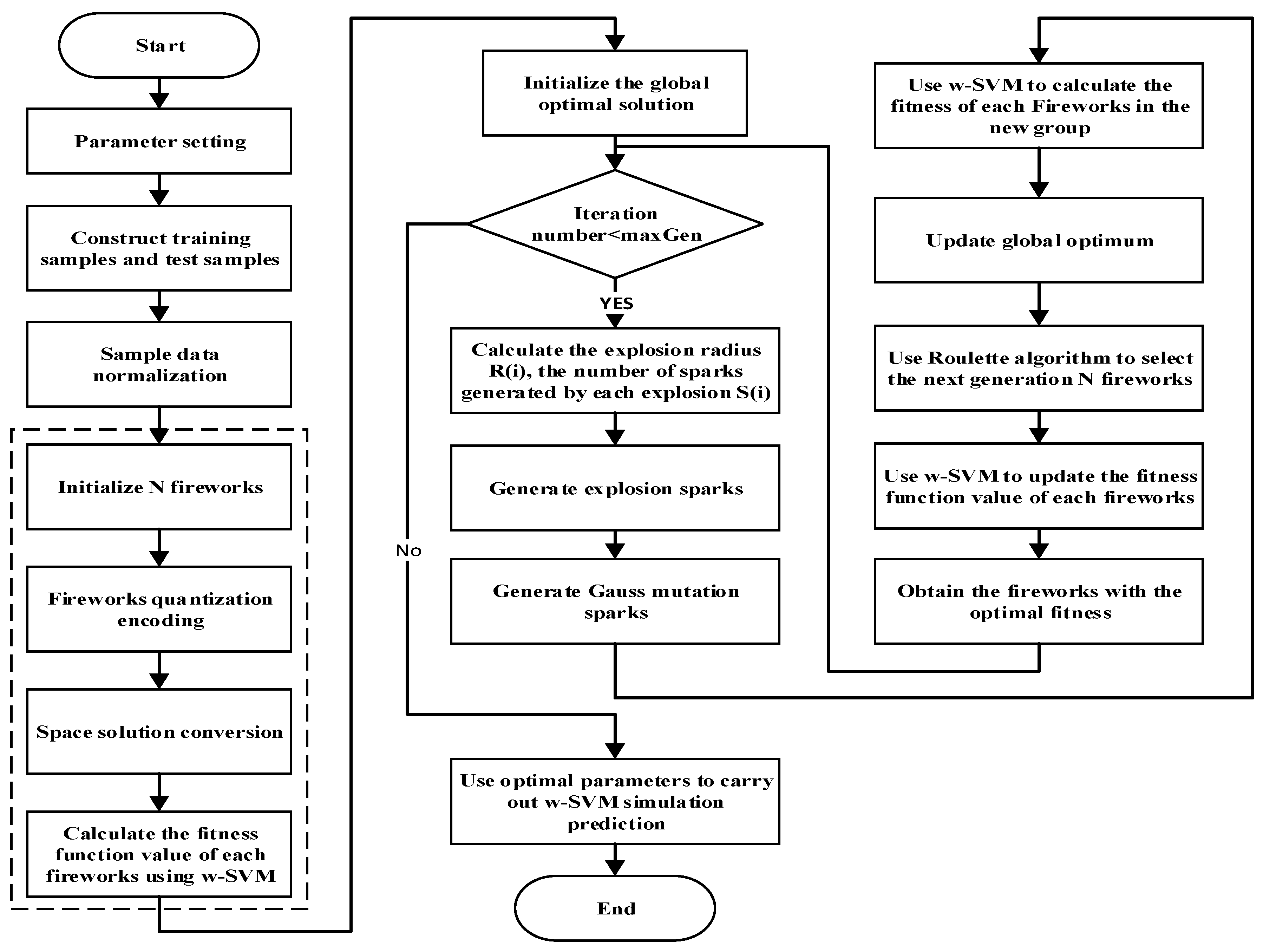
2.3. Quantum Fireworks Algorithm for Parameters Selection of Wavelet Support Vector Machine (w-SVM) Model
- (1)
- Initialize the parameters. Initialize the number of fireworks , the explosion radius , the number of explosive sparks , the mutation probability , the maximum number of iterations , the upper and lower bound of the solution space and respectively, and so on.
- (2)
- Separate the sample date as training samples and test samples, then normalize the sample data.
- (3)
- Initialize the solution space.
- In the solution space, randomly initialize positions, that is, fireworks. Each of the fireworks has two dimensions, that is, and .
- Use the probability amplitude of quantum bits to encode current position of fireworks according to Equations (9)–(10).
- Converse the Solution space according to Equations (11)–(12).
- Input the training samples, use w-SVM to carry out a training simulation for each fireworks, and calculate the value of the fitness function corresponding to each of the fireworks.
- (4)
- Initialize the global optimal solution by using the above initialized solution space, including the global optimal phase, the global optimal position quantization of fireworks, the global best fireworks, and the global best fitness value.
- (5)
- Start iteration and stop the cycle when the maximum number of iterations is achieved.
- According to the fitness value of each firework, calculate the corresponding explosion radius and the number of sparks generated by each explosion. The purpose of calculating and is to obtain the optimal fitness values, which means that if the fitness value is smaller, the explosion radius is larger, and the number of sparks generated by each explosion is bigger. Therefore, more excellent fireworks can be retained as much as possible.
- Generate the explosive sparks. When each fireworks explodes, carry out the solution space conversion for each explosion spark and control their spatial positions through cross border detection.
- Generate Gaussian mutation sparks. Carry out a fireworks mutation operation according to Equations (26)–(27), resulting in mutation sparks.
- Use the initial fireworks, explosive sparks and Gauss mutation sparks to establish a group, and the fitness value of each firework in the new group is calculated by using w-SVM.
- Update the global optimal phase, the global optimal position quantization of fireworks, the global best fireworks, and the global best fitness value.
- Use roulette algorithm to choose the next generation of fireworks, and obtain the next generation of N fireworks.
- Use w-SVM to carry out a training simulation for each fireworks, and update the value of the fitness function corresponding to each of the fireworks.
- (6)
- After all iterations, the best fireworks can be obtained, which correspond to the best parameters of and .
3. Case Study and Results Analysis
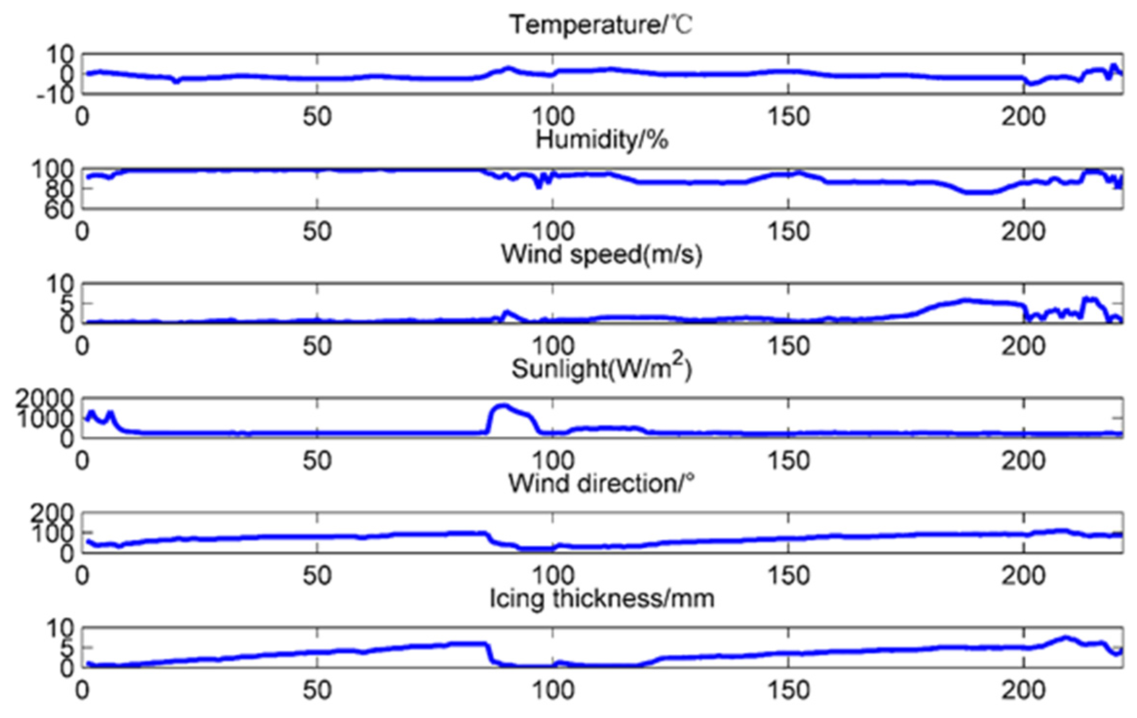
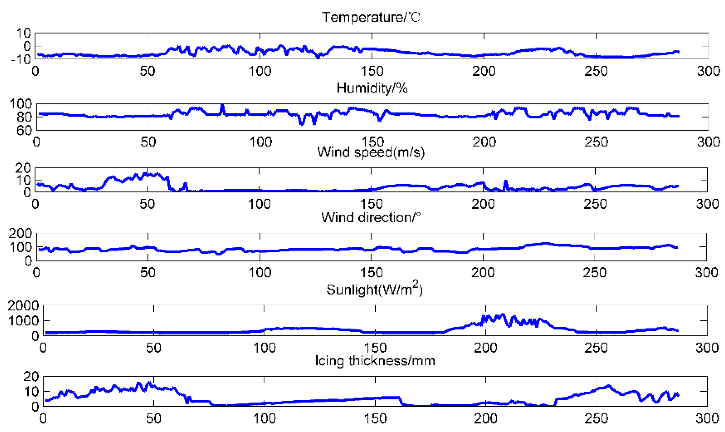
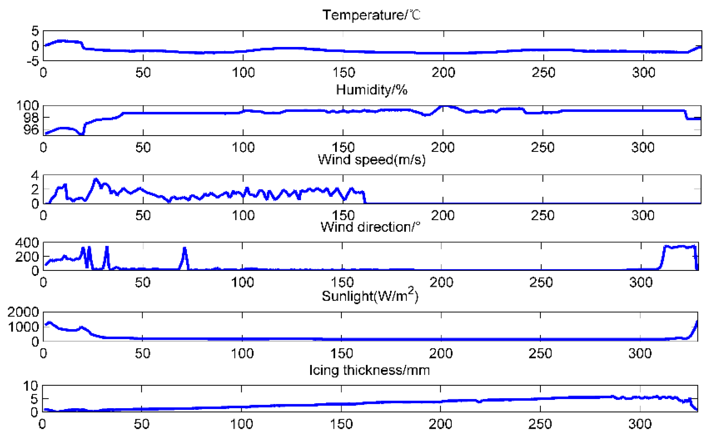
3.1. Data Selection
3.2. Data Pre-Treatment
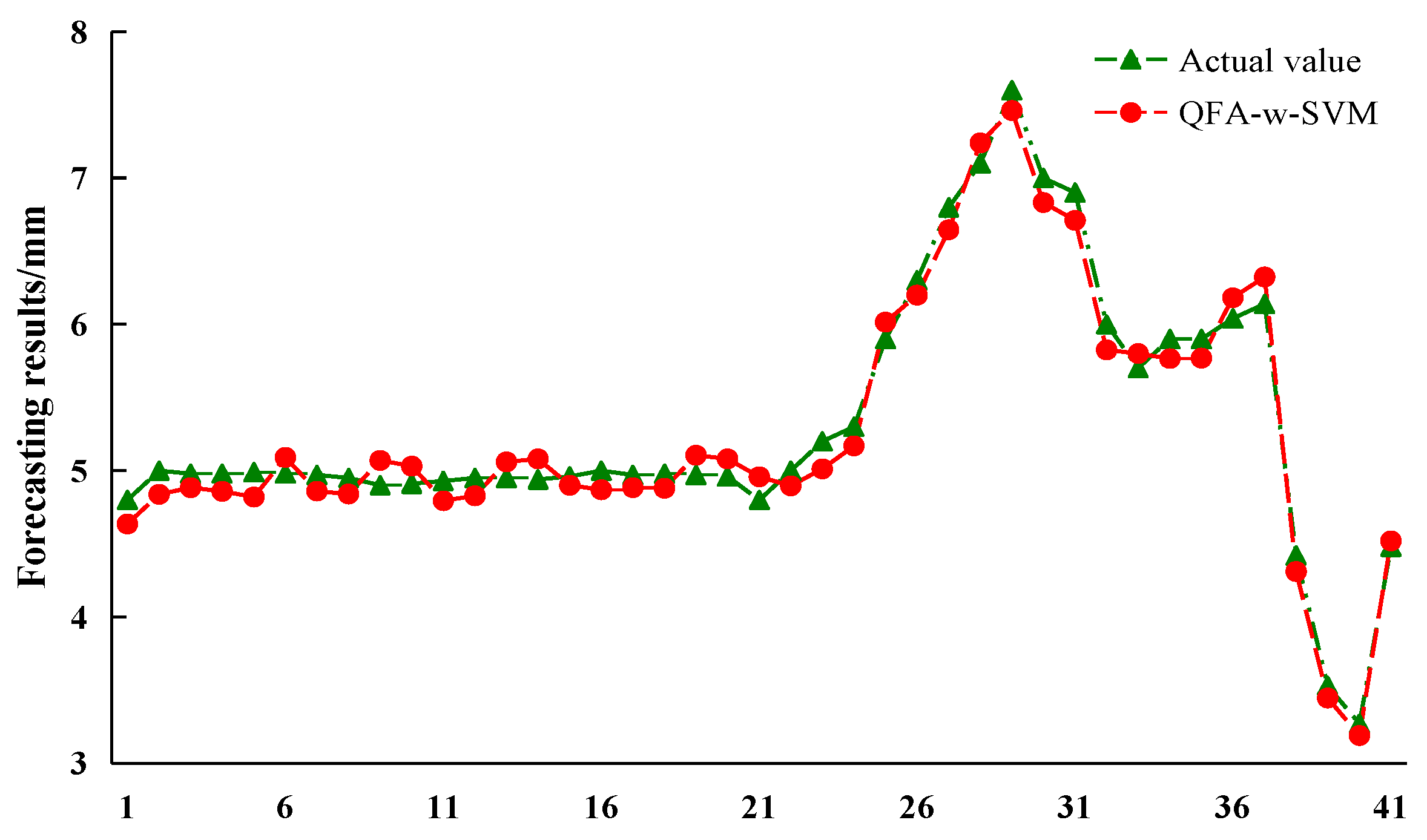
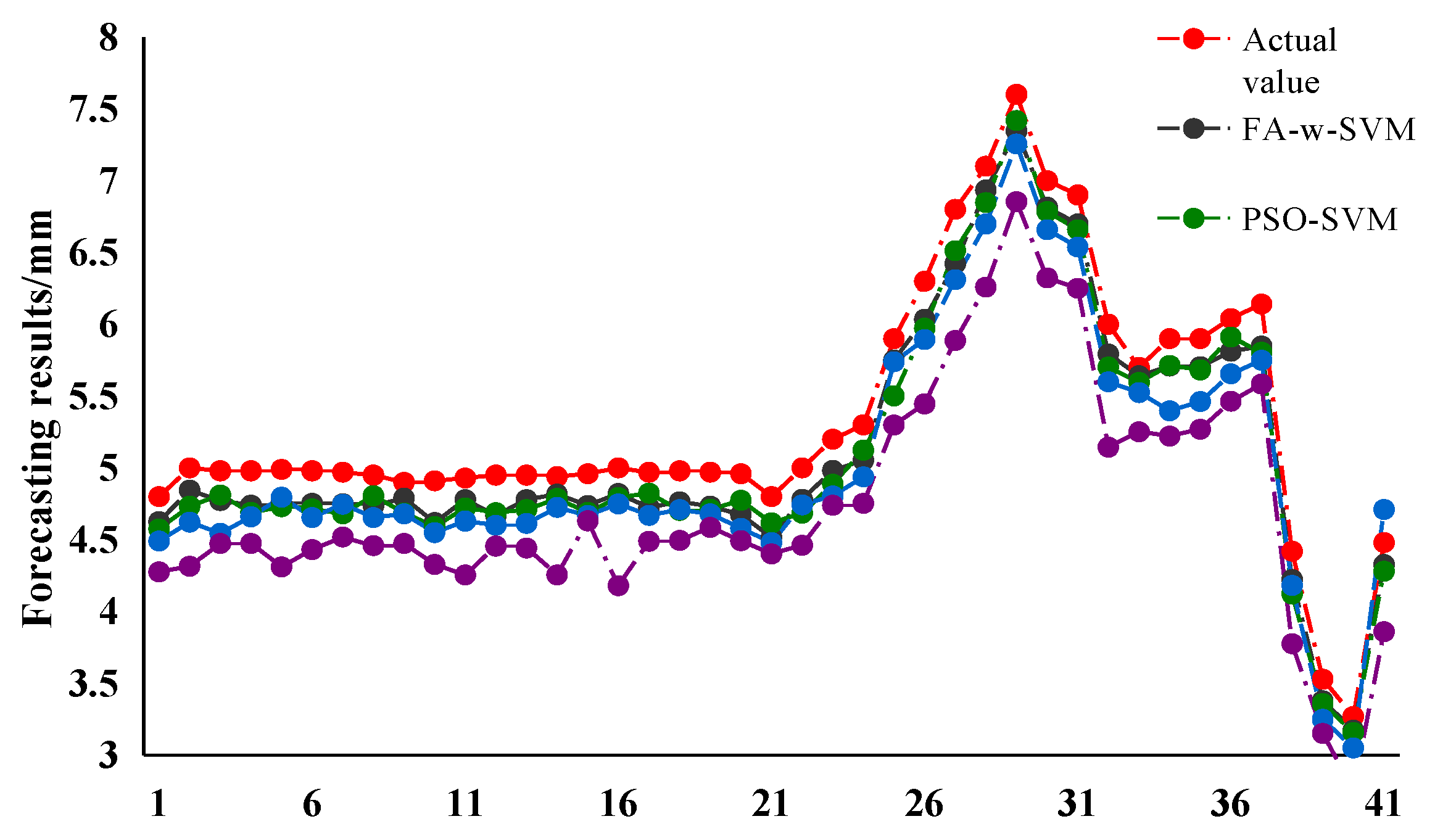
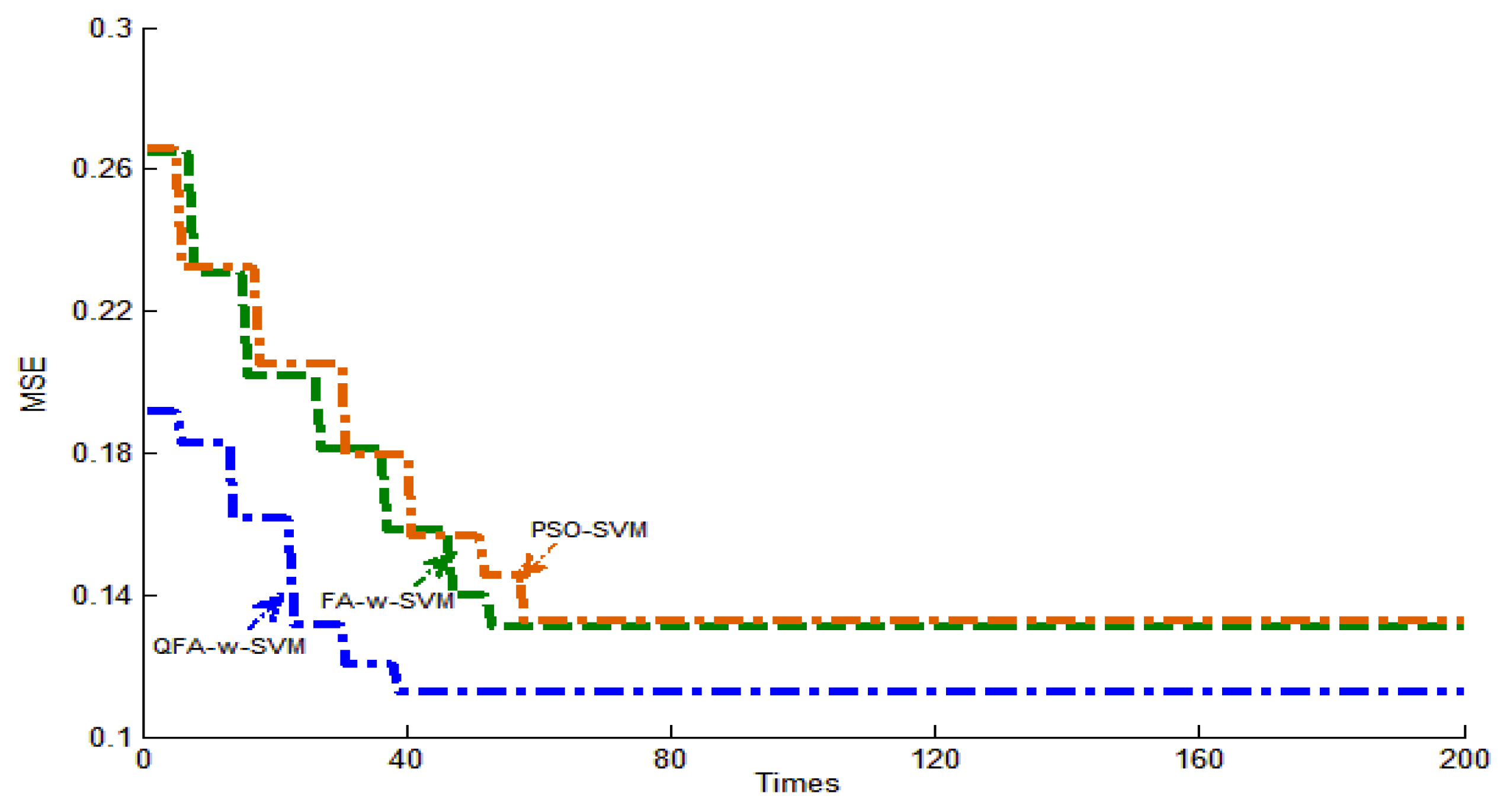
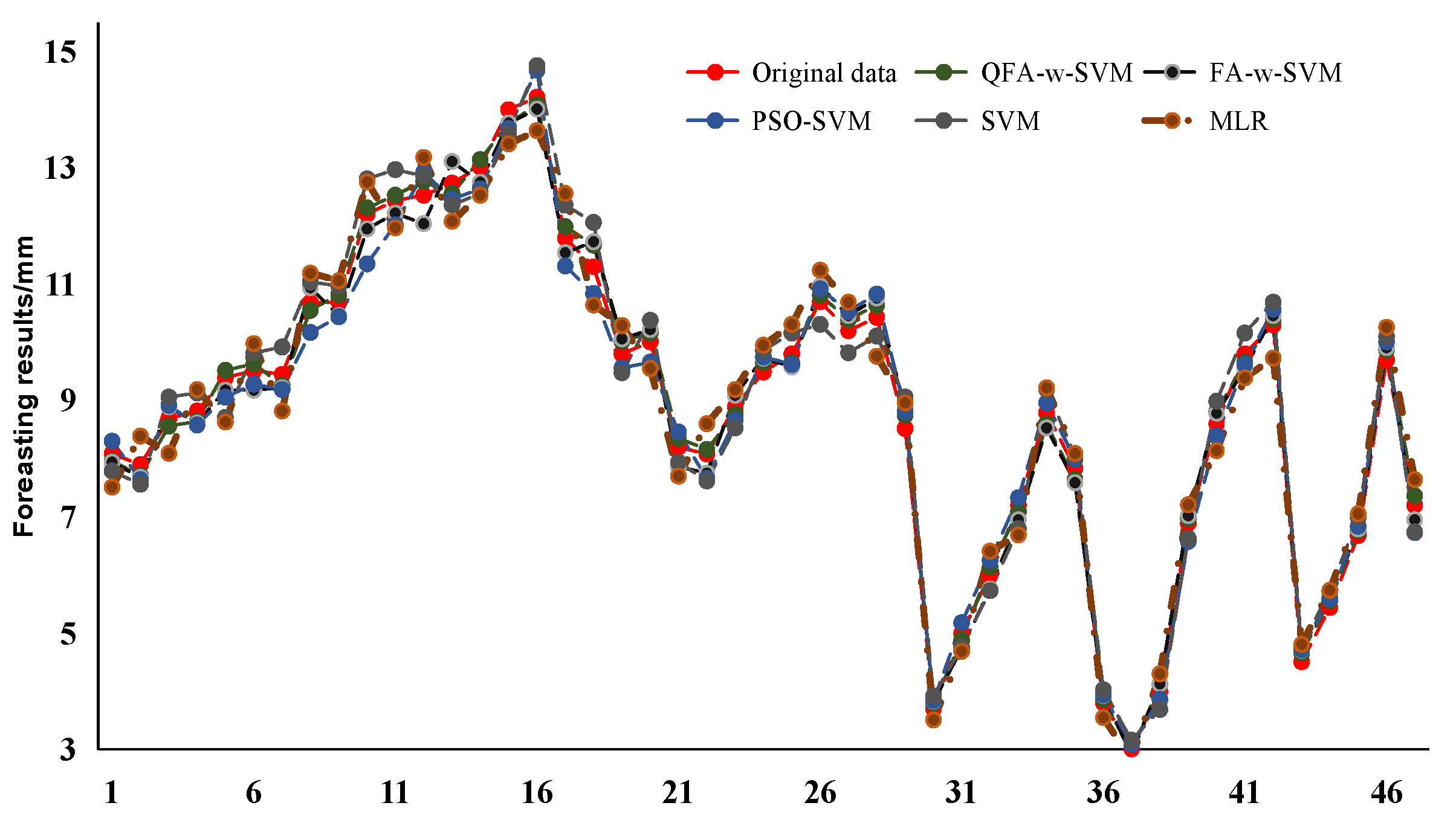
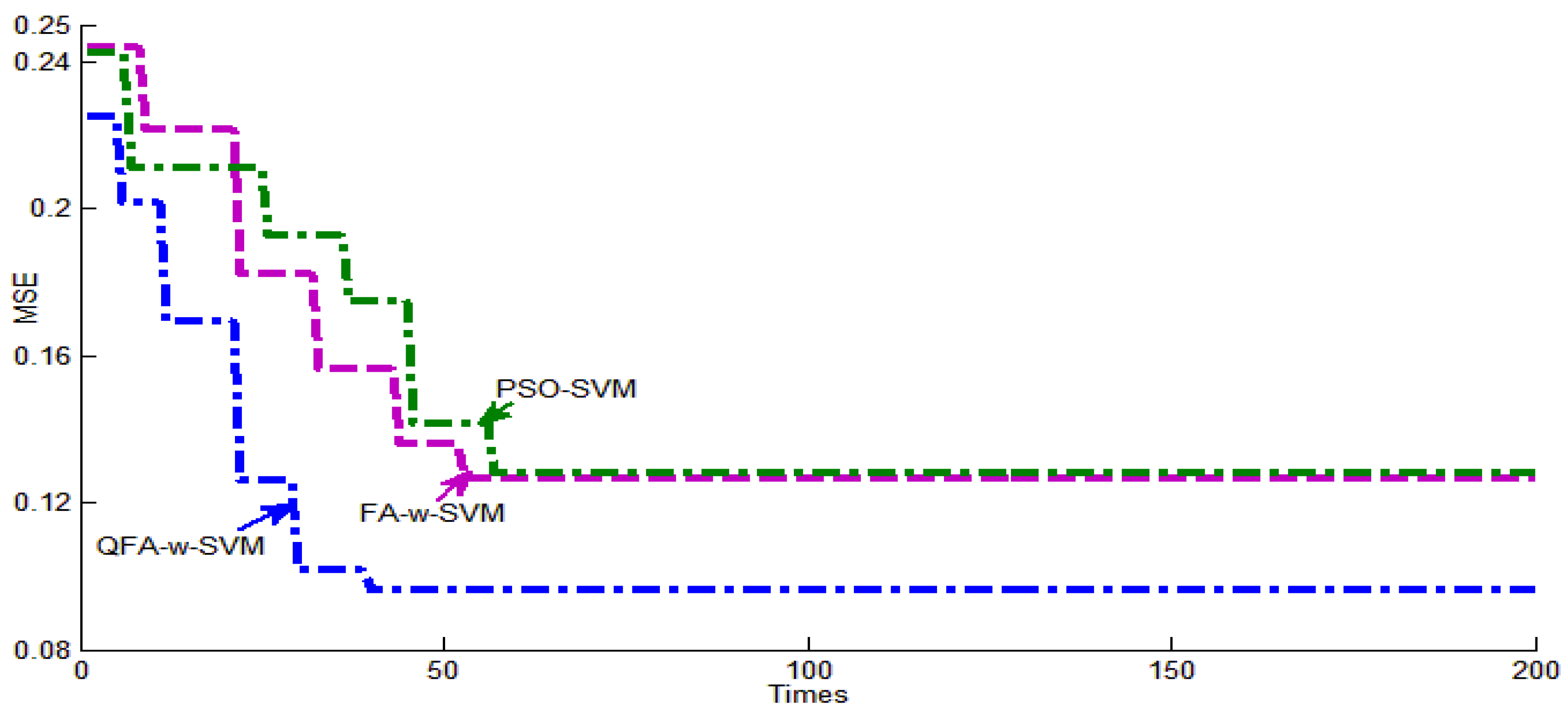
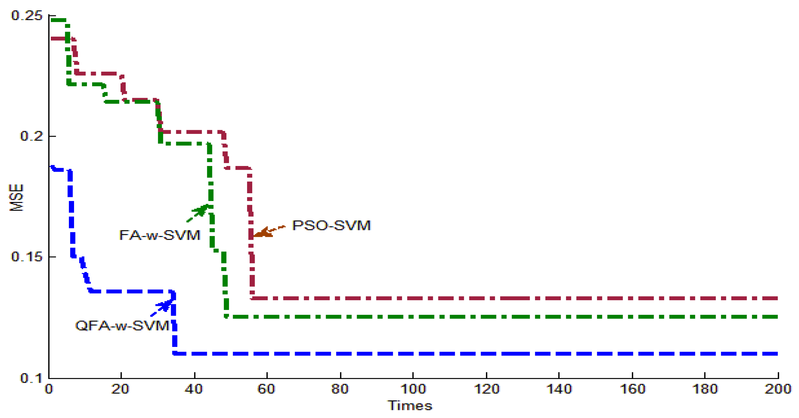
3.3. Case Study 1
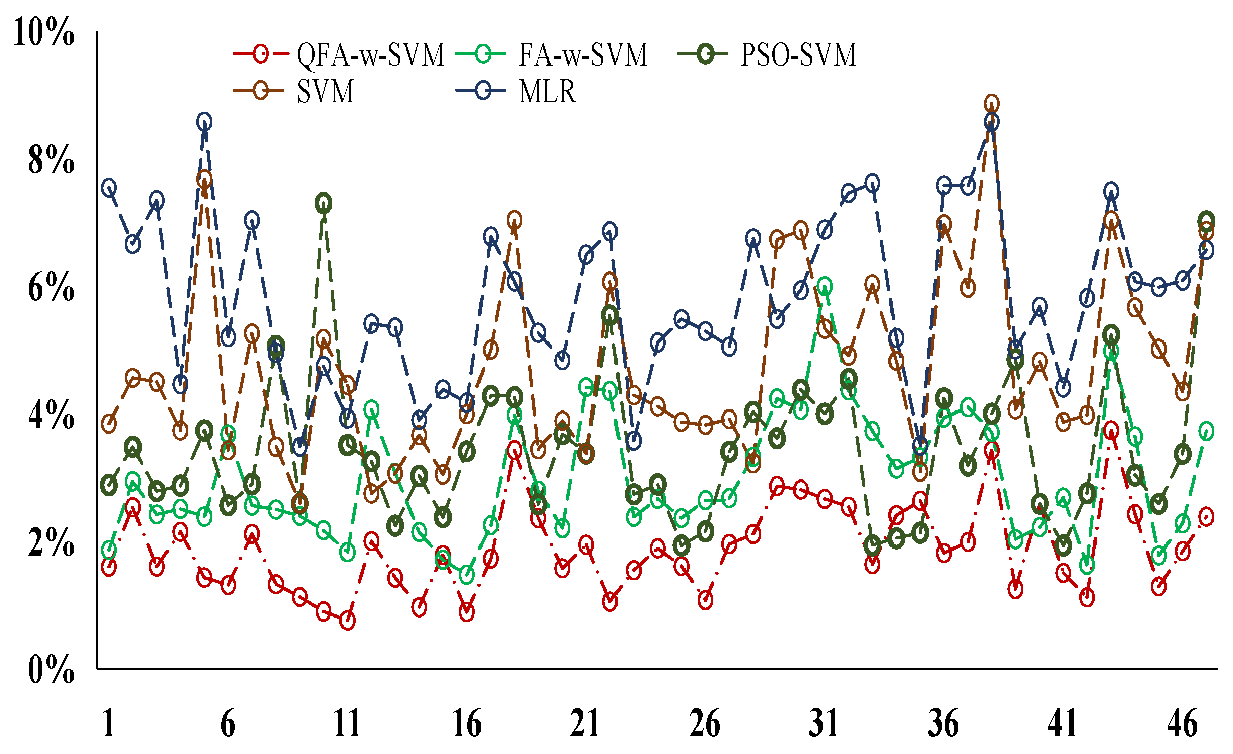
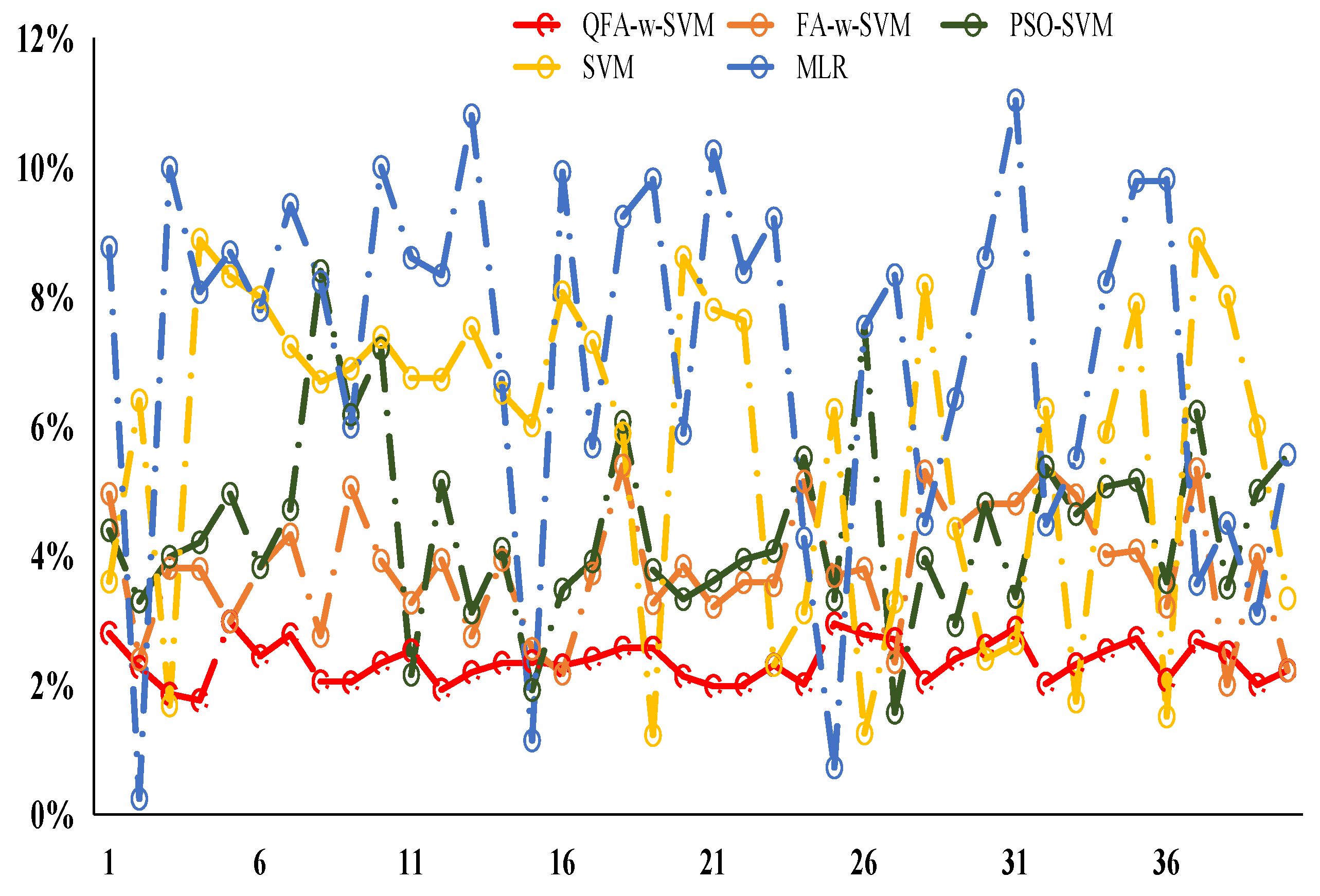
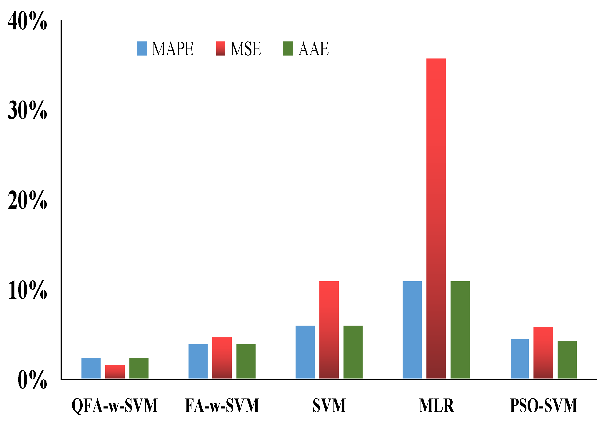
3.4. Case Study 2
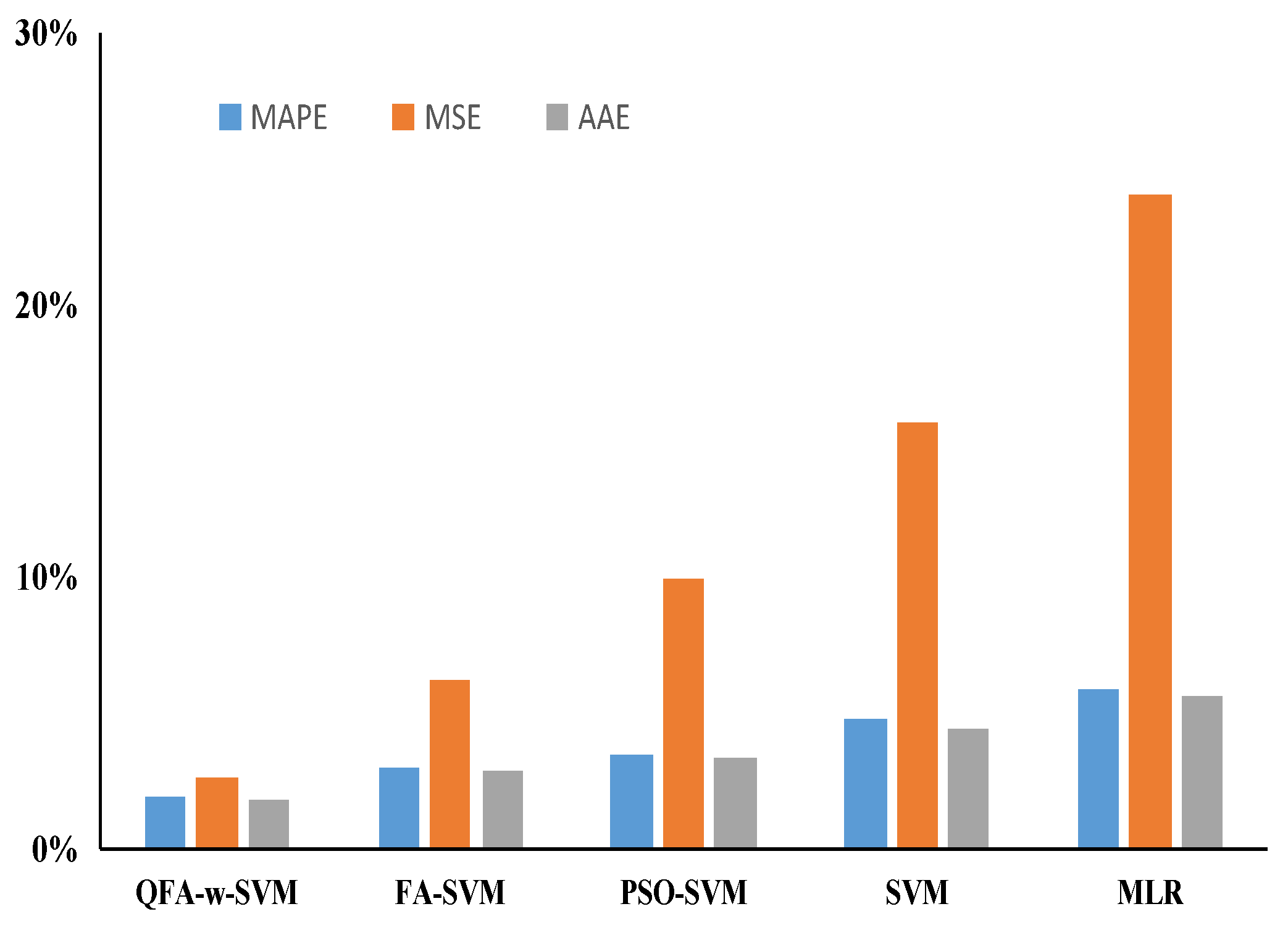
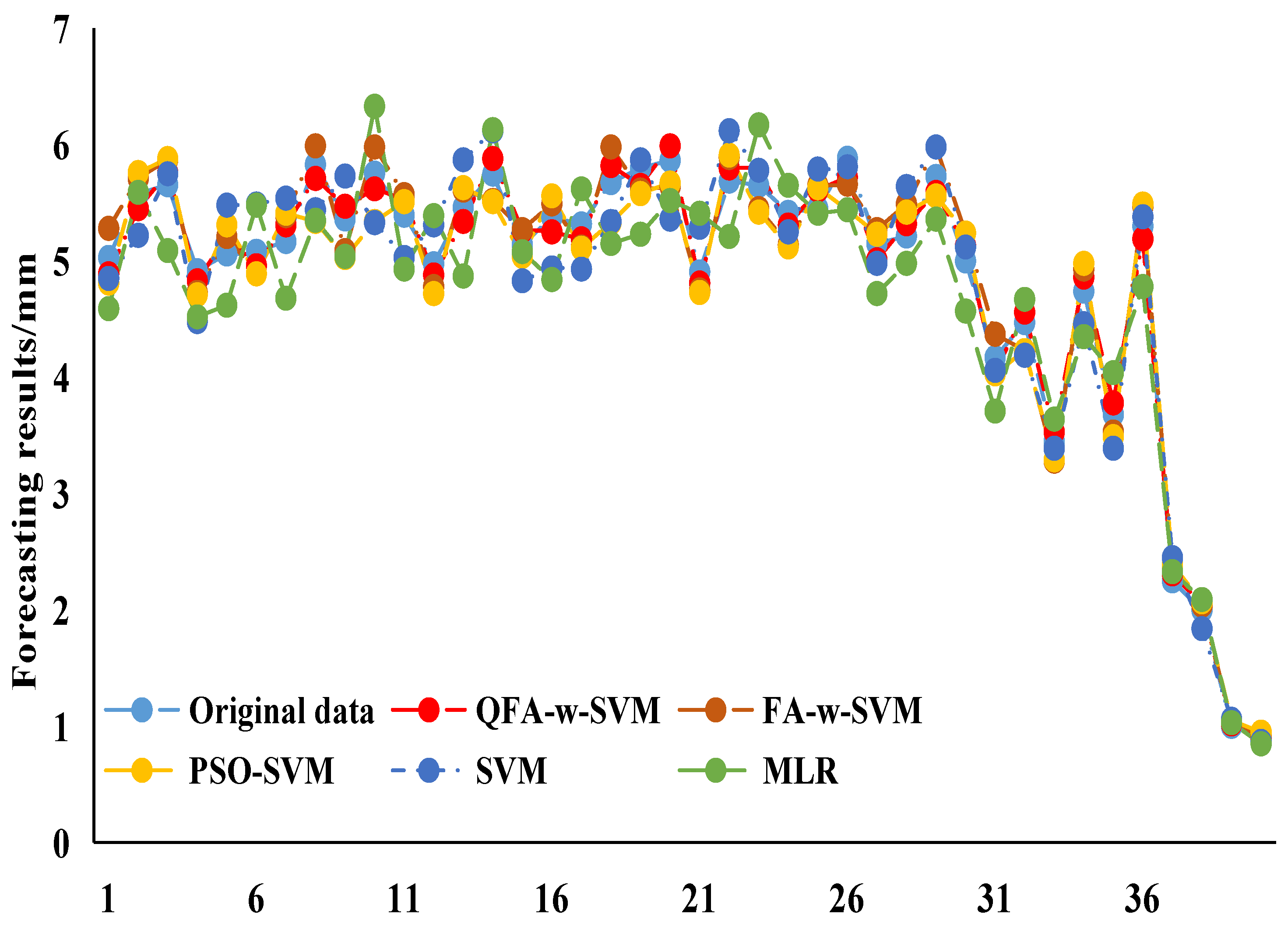
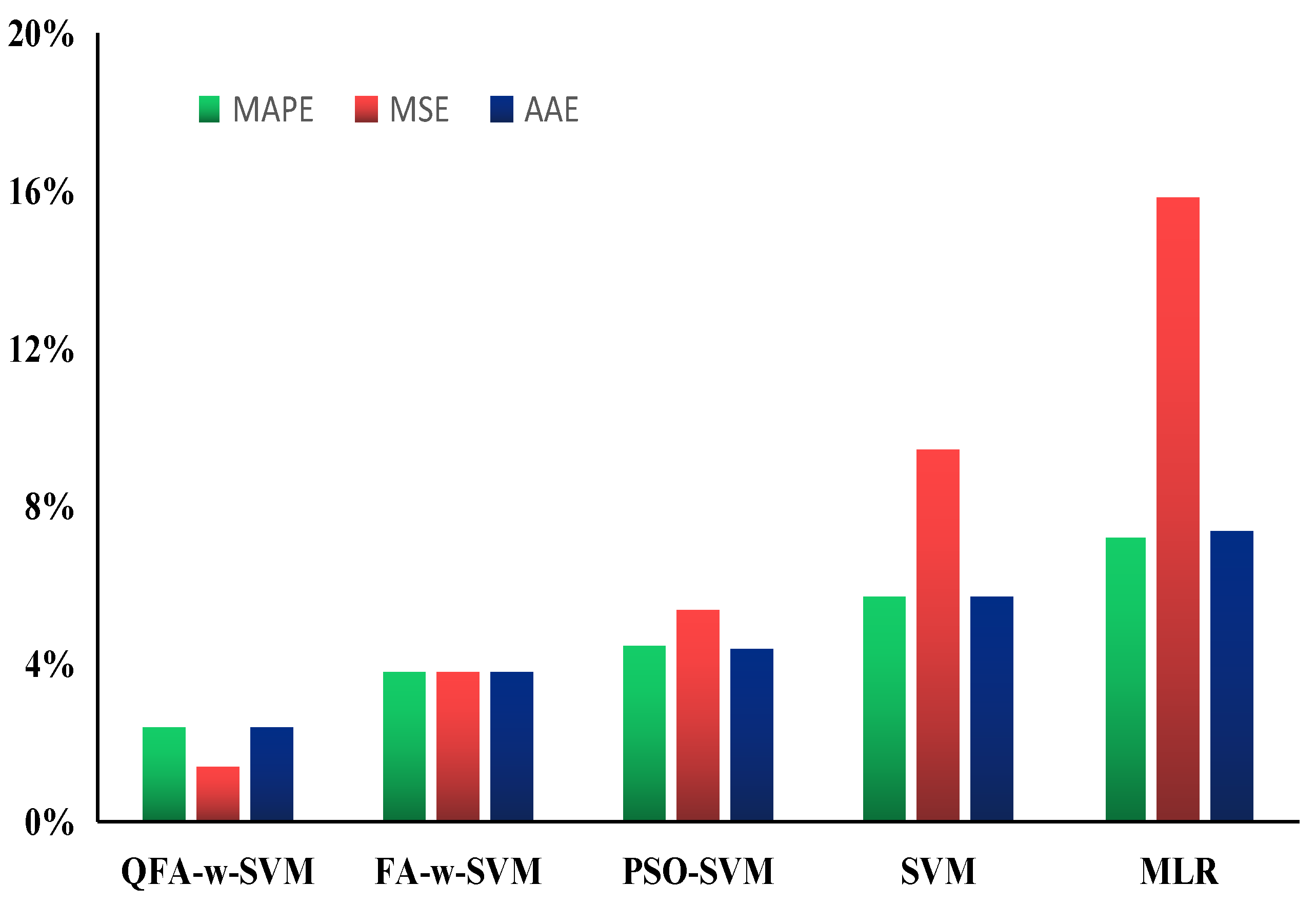
3.5. Case Study 3
4. Conclusions
Author Contributions
Acknowledgments
Conflicts of Interest
Reference
- Yin, S.; Lu, Y.; Wang, Z.; Li, P.; Xu, K.J. Icing Thickness forecasting of overhead transmission line under rough weather based on CACA-WNN. Electr. Power Sci. Eng. 2012, 28, 28–31. [Google Scholar]
- Jia-Zheng, L.U.; Peng, J.W.; Zhang, H.X.; Li, B.; Fang, Z. Icing meteorological genetic analysis of hunan power grid in 2008. Electr. Power Constr. 2009, 30, 29–32. [Google Scholar]
- Goodwin, E.J.I.; Mozer, J.D.; Digioia, A.M.J.; Power, B.A. Predicting ice and snow loads for transmission line design. 1983; 83, 267–276. [Google Scholar]
- Makkonen, L. Modeling power line icing in freezing precipitation. Atmos. Res. 1998, 46, 131–142. [Google Scholar] [CrossRef]
- Liao, Y.F.; Duan, L.J. Study on estimation model of wire icing thickness in hunan province. Trans. Atmos. Sci. 2010, 33, 395–400. [Google Scholar]
- Sheng, C.; Dong, D.; Xiaotin, H.; Muxia, S. Short-term Prediction for Transmission Lines Icing Based on BP Neural Network. In Proceedings of the 2012 IEEE Asia-Pacific Power and Energy Engineering Conference (APPEEC), Sanya, China, 31 December 2012–2 January 2013; pp. 1–5.
- Liu, J.; Li, A.-J.; Zhao, L.-P. A prediction model of ice thickness based on T-S fuzzy neural networks. Hunan Electr. Power 2012, 32, 1–4. [Google Scholar]
- Du, X.; Zheng, Z.; Tan, S.; Wang, J. The study on the prediction method of ice thickness of transmission line based on the combination of GA and BP neural network. In Proceedings of the 2010 International Conference on IEEE E-Product E-Service and E-Entertainment (ICEEE), Henan, China, 7–9 November 2010; pp. 1–4.
- Zarnani, A.; Musilek, P.; Shi, X.; Ke, X.D.; He, H.; Greiner, R. Learning to predict ice accretion on electric power lines. Eng. Appl. Artif. Intell. 2012, 25, 609–617. [Google Scholar] [CrossRef]
- Huang, X.-T.; Xu, J.-H.; Yang, C.-S.; Wang, J.; Xie, J.-J. Transmission line icing prediction based on data driven algorithm and LS-SVM. Autom. Electr. Power Syst. 2014, 38, 81–86. [Google Scholar]
- Li, Q.; Li, P.; Zhang, Q.; Ren, W.P.; Cao, M.; Gao, S.F. Icing load prediction for overhead power lines based on SVM. In Proceedings of the 2011 International Conference on IEEE Modelling, Identification and Control (ICMIC), Shanghai, China, 26–29 June 2011; pp. 104–108.
- Li, J.; Dong, H. Modeling of chaotic systems using wavelet kernel partial least squares regression method. Acta Phys. Sin. 2008, 57, 4756–4765. [Google Scholar]
- Wu, Q. Hybrid model based on wavelet support vector machine and modified genetic algorithm penalizing Gaussian noises for power load forecasts. Expert Syst. Appl. 2011, 38, 379–385. [Google Scholar] [CrossRef]
- Liao, R.J.; Zheng, H.B.; Grzybowski, S.; Yang, L.J. Particle swarm optimization-least squares support vector regression based forecasting model on dissolved gases in oil-filled power transformers. Electr. Power Syst. Res. 2011, 81, 2074–2080. [Google Scholar] [CrossRef]
- Dos Santosa, G.S.; Justi Luvizottob, L.G.; Marianib, V.C.; Dos Santos, L.C. Least squares support vector machines with tuning based on chaotic differential evolution approach applied to the identification of a thermal process. Expert Syst. Appl. 2012, 39, 4805–4812. [Google Scholar] [CrossRef]
- Tan, Y.; YU, C.; Zheng, S.; Ding, K. Introduction to fireworks algorithm. Int. J. Swarm Intell. Res. 2013, 4, 39–70. [Google Scholar] [CrossRef]
- Gao, J.; Wang, J. A hybrid quantum-inspired immune algorithm for multiobjective optimization. Appl. Math. Comput. 2011, 217, 4754–4770. [Google Scholar] [CrossRef]
- Wang, J.; Li, L.; Niu, D.; Tan, Z. An annual load forecasting model based on support vector regression with differential evolution algorithm. Appl. Energy 2012, 94, 65–70. [Google Scholar] [CrossRef]
- Dai, H.; Zhang, B.; Wang, W. A multiwavelet support vector regression method for efficient reliability assessment. Reliab. Eng. Syst. Saf. 2015, 136, 132–139. [Google Scholar] [CrossRef]
- Kang, J.; Tang, L.W.; Zuo, X.Z.; Li, H.; Zhang, X.H. Data prediction and fusion in a sensor network based on grey wavelet kernel partial least squares. J. Vib. Shock 2011, 30, 144–149. [Google Scholar]


© 2016 by the authors; licensee MDPI, Basel, Switzerland. This article is an open access article distributed under the terms and conditions of the Creative Commons by Attribution (CC-BY) license (http://creativecommons.org/licenses/by/4.0/).
Share and Cite
Ma, T.; Niu, D.; Fu, M. Icing Forecasting for Power Transmission Lines Based on a Wavelet Support Vector Machine Optimized by a Quantum Fireworks Algorithm. Appl. Sci. 2016, 6, 54. https://doi.org/10.3390/app6020054
Ma T, Niu D, Fu M. Icing Forecasting for Power Transmission Lines Based on a Wavelet Support Vector Machine Optimized by a Quantum Fireworks Algorithm. Applied Sciences. 2016; 6(2):54. https://doi.org/10.3390/app6020054
Chicago/Turabian StyleMa, Tiannan, Dongxiao Niu, and Ming Fu. 2016. "Icing Forecasting for Power Transmission Lines Based on a Wavelet Support Vector Machine Optimized by a Quantum Fireworks Algorithm" Applied Sciences 6, no. 2: 54. https://doi.org/10.3390/app6020054