Article

Dynamic Characterization of Cohesive Material Based on Wave Velocity Measurements

1
Water Centre Laboratory, Faculty of Civil and Environmental Engineering, Warsaw University of Life Sciences, 02-787 Warsaw, Poland
2
Department of Geotechnical Engineering, Faculty of Civil and Environmental Engineering, Warsaw University of Life Sciences, 02-787 Warsaw, Poland
*
Author to whom correspondence should be addressed.
Appl. Sci. 2016, 6(2), 49; https://doi.org/10.3390/app6020049
Submission received: 29 October 2015 / Revised: 14 January 2016 / Accepted: 15 January 2016 / Published: 9 February 2016
(This article belongs to the Special Issue Acoustic and Elastic Waves: Recent Trends in Science and Engineering)

Abstract

:
The paper presents a description of the dynamic properties of cohesive material, namely silty clays, obtained by using one of the applied seismology methods, the bender elements technique. The authors’ aim was to present the dynamics of a porous medium, in particular an extremely important passage of seismic waves that travel through the bulk of a medium. Nowadays, the application of the bender element (BE) technique to measure, e.g., small strain shear stiffness of soils in the laboratory is well recognized, since it allows for reliable and relatively economical shear wave velocity measurements during various laboratory experiments. However, the accurate estimation of arrival time during BE tests is in many cases unclear. Two different interpretation procedures (from the time domain) of BE tests in order to measure travel times of waves were examined. Those values were then used to calculate shear and compression wave velocities and elastic moduli. Results showed that the dynamic parameters obtained by the start-to-start method were always slightly larger (up to about 20%) than those obtained using the peak-to-peak one. It was found that the peak-to-peak method led to more scattered results in comparison to the start-to-start method. Moreover, the influence of the excitation frequency, the mean effective stress and the unloading process on the dynamic properties of the tested material was studied. In addition, the obtained results highlighted the importance of initial signal frequency and the necessity to choose an appropriate range of frequencies to measure the shear wave velocity in clayey soils.

Graphical Abstract

1. Introduction

The determination of seismic velocities, as well as the elasticity modulus and structural properties of porous materials plays an extremely important role in the development of various engineering projects [1]. The small strain and elastic moduli, such as the shear modulus (Gmax) and Young’s modulus (Emax), are key parameters during, for example, the site response analysis of an earthquake, the design of machine foundations and soil dynamics problems [2]. Burland et al. [3] even emphasized the significance of Gmax in static deformation analysis of geotechnical problems. Usually, the above-mentioned elastic modulus of soil deposits is measured in situ by means of so-called seismic exploration [4]. In order to evaluate the shear modulus (G) or Young’s modulus (E) values in the laboratory, triaxial or torsional shear testing machines, which employ what is generally known as the static loading methods [5], are applied. Other kinds of evaluation methods, commonly referred to as vibration test methods, are those relying on applying wave motions to the test specimens and then observing their behavior during the resonance, including free oscillation time. A great example is a resonant column apparatus. Apart from this, there are also pulse transmission techniques, which include the ultrasonic pulse test, bender element (BE), etc. They allow calculating Gmax at small strains on the basis of the wave velocity [6].
Some of the laboratory tests and field studies, such as cross-hole seismic [7,8], down-hole seismic [9], suspension logging [10], seismic cone [11], seismic flat dilatometer [12] and spectral analysis of seismic waves [13], are indirect tests [14]. Compared to direct tests, the indirect tests enable measuring quantities different from the more desired ones and relate them to each other through mathematical relationships. Seismic techniques are classified as indirect testing methods for small strain stiffness [7]. They yield profiles of wave propagation velocity. When we assume that the behavior of the material is linear-elastic, this means that elastic stiffness relates to wave propagation velocity following the equations below:
υ P = λ + 2 G ρ
υ S = G ρ
where υP is the propagation velocity of pressure, which might as well be called a primary (P-) wave velocity, υS is the propagation velocity of shear or the secondary (S-) wave and λ and G are Lame’s constants (another term for G is the shear modulus). For engineers, it is more convenient to express Lame’s constant as a function of Young’s modulus and Poisson’s ratio in accordance with these equations:
G = E 2 ( 1 + ν )
λ = ν E ( 1 + ν ) ( 1 2 ν )
Figure 1 illustrates the particle motion in P- and S-waves.
Figure 1. P-wave (top) and S-wave (bottom) particle motion. The particle motion in P-waves is longitudinal, while in S-waves, it is transverse. The particle motion vector in the plane perpendicular to the direction of propagation is referred to as polarization (only in the case of S-waves) [8].
Applsci 06 00049 g001
Over the years, bender elements have become increasingly popular in order to determine the S-wave velocity [9,10] through experiments. Nowadays, they are commonly available [11,12]. Bender elements consist of two sheets produced from piezoceramic plates, which are rigidly bonded, to a center brass shim or stainless steel plate. Because of their piezoelectric properties, they are capable of converting mechanical excitation into electrical output and vice versa. When excited by an input voltage, the bender element changes its shape, which is accompanied by mechanical excitation. Because of this fact, it acts as a signal transmitter. Being subjected to mechanical excitation causes the emission of an electrical output by another bender element, which is, in this way, acting as a signal receiver [9]. The first person to use piezoceramic elements bonded to shear plates was probably Lawrence [13,14]. His idea was to measure the velocity of the shear wave in materials, such as clay and sand. In 1978, Shirley [15] proposed the introduction of piezoceramic bender elements to determine S-wave velocity in the laboratory. Other scientists, like Dyvik and Madshus [16], described the incorporation of BE for geotechnical laboratory testing in the 1980s.
The appeal of the BE technique lies in its apparent simplicity: one of the transducers is excited at one end of a specimen by a single pulse excitation, and the second, located at the other end of a specimen, is receiving it. The time required for this process can be simply read off from an oscilloscope. On the basis of this value, shear wave velocity can be obtained [17]. Therefore, BEs are an inexpensive and versatile solution, which can be used for laboratory seismic measurement. Furthermore, their capabilities of monitoring the process of stiffening with effective stresses, namely cementation, load stabilization, curing or consolidation, are particularly appealing [18]. However, there is a critical drawback connected with a BE test that contributes to many errors, namely the determination of the travel time. A number of researchers, including Viggiani and Atkinson (1995), attempted to use various methods in order to find the arrival time in order to reduce the degree of subjectivity [19]. In 2005, Lee and Santamarina [20], as well as Leong et al. [21] reported a method of travel time determination, by performing a bender element test. Nevertheless, there are still some differences between the first arrival of the S-wave and the preferred input wave. Therefore, the BE technique still needs to be verified with respect to how reliable it is, when it comes to calculation of the arrival time [2,22].
The intention of the authors of this paper was to recognize the dynamic characteristics of the cohesive medium through the performance of the BE tests on this material, i.e., clayey soil, obtained from the area of Warsaw, the capital of Poland, at various effective confining pressures under saturated conditions. Two methods, namely peak-to-peak and start-to-start, were used to determine the travel time using the BE technique. The υS was calculated on this basis. Subsequently, shear modulus (G) was obtained using the value of shear wave velocity. Additionally, the authors used piezoceramic elements to determine compression wave velocity (υP). Furthermore, they tried to evaluate the values of dynamic Poisson’s ratio (νd). The dynamic Poisson’s ratio of soil deposits is a matter that has attracted rather little attention so far [23]. Nevertheless, it significantly affects stresses, strains, wave propagation characteristics in a mass of soils and other important types of soil deposit behavior during dynamic excitation [4]. In this paper, νd was calculated from the results of measurements of longitudinal and shear wave velocities in seismic exploration and then used to establish Young’s modulus (E). The authors also studied the possible impact of unloading on the received values of elastic modulus.

2. Methods and Materials
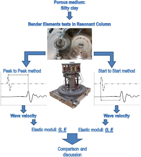
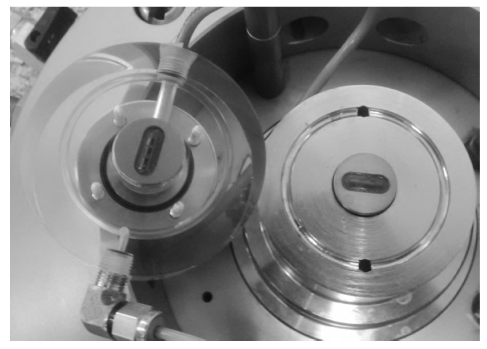
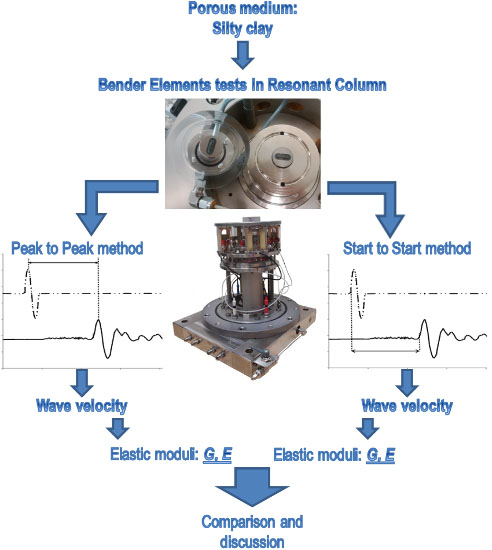
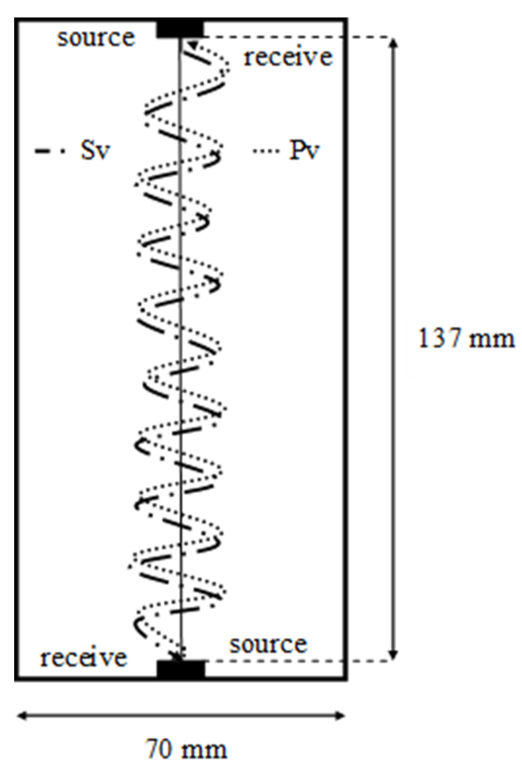
2.1. Test Equipment

For the experiments, the authors employed a Stokoe fixed-free type of resonant column, manufactured in 2009 by the British company GDS Instruments Ltd, with its office in Hook, Hampshire, U.K. A detailed description of this device is contained in the authors’ other publications [24,25] and will not be discussed in this paper. The BEs, produced as well by GDS Instruments Ltd in 2009, were installed in the above-mentioned resonant column apparatus. The GDS bender elements are made from piezoelectric ceramic bimorphs. Two sheets are bonded together with a metal shim in between them. Excitation voltage is used to produce a displacement in the source transducer, resulting in a wave being sent through the sample. This wave generates a displacement in the receiver, which induces a voltage that can be measured.
The GDS bender elements come in the form of an insert that can be mounted in a top cap or a pedestal (Figure 2). This makes them easy to replace and able to be used with a wide range of triaxial cells. The insert for the base pedestal is made of stainless steel, while the one for the top cap is made of titanium. This reduces the weight by half and minimizes the axial load caused by the top cap, which is being applied to the sample. The inserts are embedded in a modified Perspex top cap and stainless steel base pedestal. At the same time, the top cap and the base pedestal are mounted on the specimen in the same way, as during a conventional triaxial test [26].
Figure 2. Bender element inserts mounted in a top cap and base pedestal.
Applsci 06 00049 g002
The S-wave source comprises two piezoceramic strips both polarized in the same direction. The application of an excitation voltage induces the extension of one strip and the contraction of the other, causing the strip to bend. Turning the excitation voltage in the opposite direction contributes to strips bending reversely. The two strips in the receiver are polarized in opposite directions. The P-wave source consists of two piezoceramic strips polarized conversely. When an excitation voltage is applied, strips extend simultaneously. Reversion of the excitation voltage causes the strips to contract [26].
In Figure 3, the BE arrangement adopted for the presented experiments is shown. Elements are manufactured to allow both S- and P-wave testing to be performed (in opposite propagation directions) on the same sample. The software switches input gain levels (of the received signal), sets the level of the output signal voltage and controls switching between P- and S-wave modes for our combined wave type elements [26]. In the current research, bender elements were used to obtain υVH velocities, propagating in the vertical plane (index V), polarized in the horizontal (index H). When performing a bender element test, one of its most important aspects is the phase orientation of the elements. The authors always checked the relationship between the received signals with respect to the source signal. The desirable orientation was “in-phase”. If the orientation was correct, the source and received traces were exactly “in-line”. An example of non-desirable output is presented in Figure 4. The source signal and the received one are not simultaneously upward.
Figure 3. Frontal sample view with bender element (BE) arrangement and an example of the waves’ path.
Applsci 06 00049 g003
Figure 4. Non-desirable orientation of the top cap and base pedestal element.
Applsci 06 00049 g004

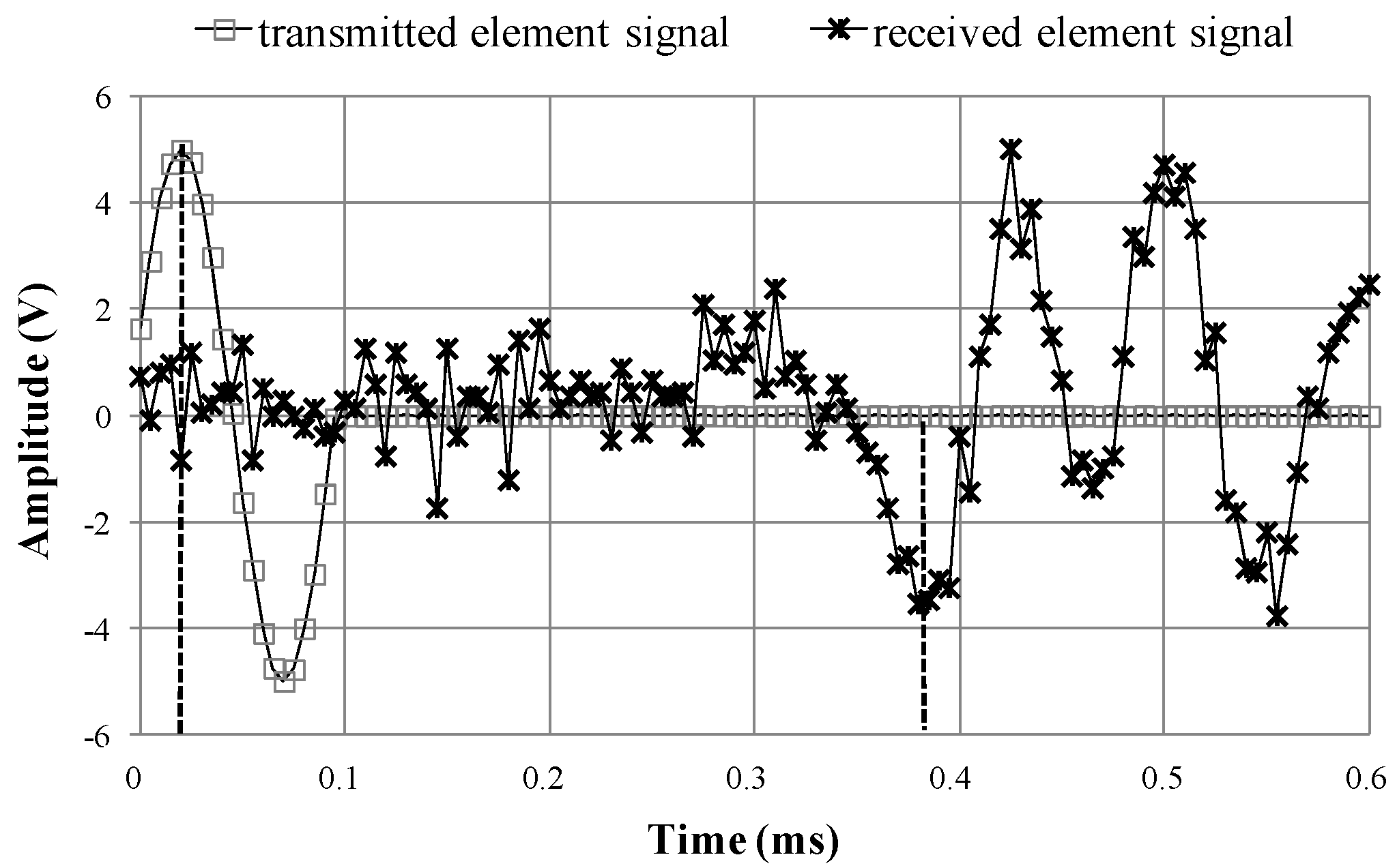
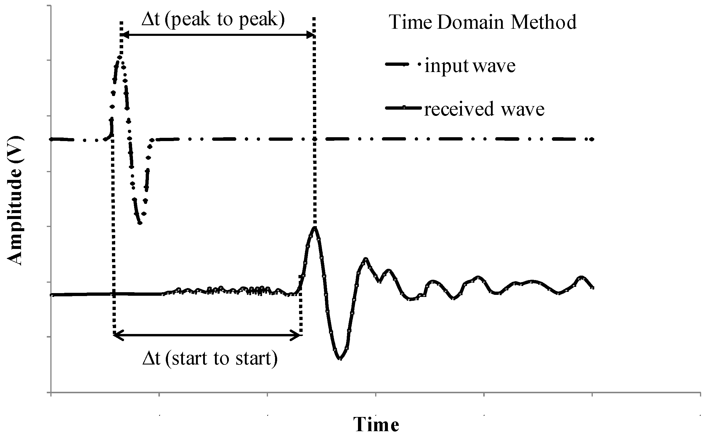
2.2. Methods of Interpretation of BE Results

The BE technique has many advantages, which have been mentioned so far, but the interpretation of BE results can often be questionable [18,22,27]. A number of methods for the analysis of bender element results are commonly used in the time or frequency domain [17,28]. The time domain methods are classified as direct measurements, which use plots of electrical signals versus time [19,29]. These methods employ a time-based axis in order to identify the propagation time, hence [6]. In frequency domain approaches, on the other hand, the spectral breakdown of the signals is analyzed, and the shift in the phase angle between the trigger and response signal is calculated [19,30]. The time domain techniques are generally simpler and more straightforward, as the travel time can be directly defined by studying the time interval between characteristic points in the transmitted and received wave traces. However, the frequency domain methods appear to be more detailed, since they employ the support of signal processing and spectrum analysis tools. Additionally, they enable automated data acquisition and processing [18]. It is important to note that no method of interpreting the BE test results is yet proven superior to the others [6,19,31]. Reliable determination of travel time is very significant, due to BEs being installed in laboratory equipment and their application for studying relatively small specimens, which means that the travel distance is quite small. Below, the authors briefly present the methods of determining the arrival time of the shear wave that were employed in the paper. These are further illustrated in Figure 5.
Figure 5. Typical identification techniques of travel time in the time domain method.
Applsci 06 00049 g005
The peak-to-peak method [19,28] is based on the assumption that the received signal bears a high resemblance to the transmitted one. The travel time may be treated as the time elapsed between any two corresponding characteristic points in the signals. By doing this, the near field problems should be reduced. The characteristic points that are most commonly used to identify the wave travel time are the first positive peak in the input of S-wave signals and in the output [32]. In some circumstances, however, properly defining the first major peak becomes quite difficult, as the received signal has several consecutive peaks, which differ slightly in amplitude. The reliability of choosing the right first peak as the first major one can be influenced by sample geometry and size or, for example, by the energy-absorbing nature of the soil. The arriving signal is then distorted to various extents due to the increase of damping with distance. The quality of received signals significantly affects this technique [28].
The principle of the start-to-start method, also known as the visual picking method, is the acceptance of the moment, when the first major deflection of the received signal occurs, as the shear wave arrival time [19,33]. The presented method is characterized by simplicity, which is the main reason behind its popularity. Depending on the installation and polarity of the bender elements, the first important deviation from zero amplitude may be positive or negative [28]. In many cases, it is simply a single sine pulse. This represents the start of energy transfer from the source to the soil. However, in case of the output wave signal, it is the moment when the investigated receiver begins exhibiting motion. Said moment represents the instant of the energy transfer from the soil to the receiving BE [32].
During the bender element test, shear wave velocity is calculated from the simple measurement of propagation distance (Δs) and propagation time (Δt). Based on a number of previous works, it is generally accepted that the travel distance is the distance between the tips of two BEs [11]. There are various waveforms, for example sine and square waves, with various frequencies, that have been recommended as an excitation signal [2].

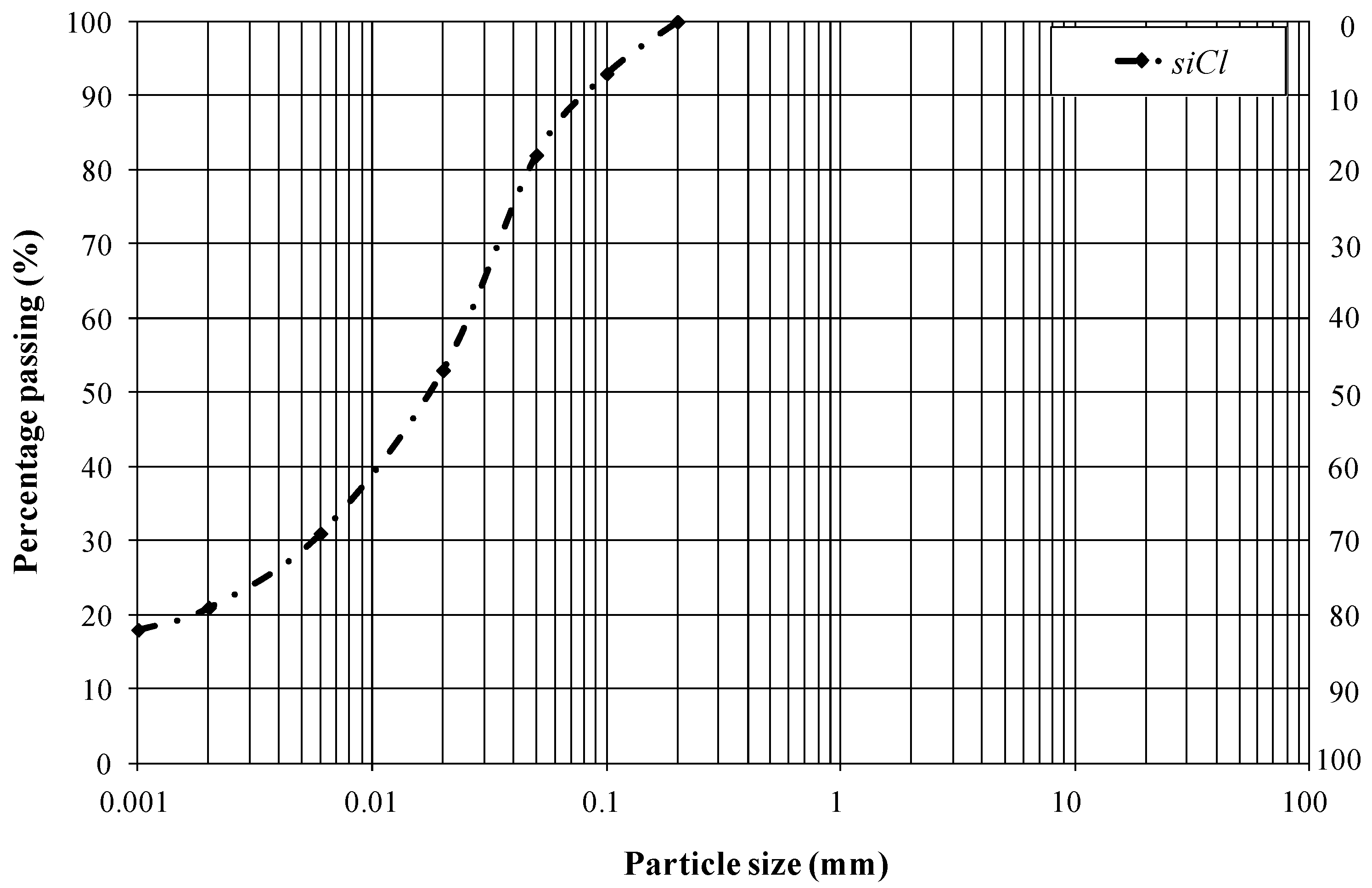
2.3. Characterization of Test Material

In order to investigate the elastic modulus of cohesive material, associated with the passage of seismic waves (an S-wave and a P-wave), silty clay (siCl) samples, from the test site located in the center of Warsaw (the capital of Poland), recognized by particle size analysis using the sieves and hydrometer methods (European Standard Eurocode 7, [34]), were used. The description of the research area can be found in [25]. The index properties of the examined soils are summarized in Table 1. In order to compute the fundamental indices (wP, wL), standard test methods were employed, namely plastic limit test of soil, Casagrande liquid limit test and fall cone liquid limit test. The grain size distribution of the soil specimens is shown in Figure 6. The proportional content of each fraction is as follows: Gr = 0%, Sa = 13%, Si = 66%, Cl = 21%. The soil used during the tests, which is of Quaternary origin, was sampled in an undisturbed state using a standard Shelby tube. All of the samples were acquired at a depth of around 6.0 m and selected cautiously with the consideration of the soil structure uniformity, their physical properties and their double phase. Tubes were pressed carefully and gently into the pre-drilled holes. Subsequently, the samples were sealed and stored in a humidity room until needed [35].
Table 1. Basic properties of the tested soils.
ParameterValue
w (%)17.52
wP (%)17.14
wL (%)33.00
IP (%)15.86
IL (%)0.02
IC (%)0.98
ρ (kg/m3)2140
w is the water content; wP is the plastic limit; wL is the liquid limit; IP is the plastic index; IL is the liquidity index; IC is the consistency index; and ρ is the mass density.
Figure 6. Grain size distribution of the tested soils.
Applsci 06 00049 g006

2.4. Test Setup and Procedure

The test procedure followed that of a drained isotropic resonant column test. An upright cylindrical specimen of soil, with an aspect ratio of 2:1 (length:diameter), was employed. The proportions between length and diameter were as follows: 140 mm × 70 mm. Undisturbed material was set up in the resonant column cell, then saturated by the back pressure method in order to achieve the level of full saturation and subsequently consolidated to predetermined isotropic stress levels of 30, 120, 180, 240, 360 and 410 kPa. Back pressure was increased slowly, in order to ensure the proper saturation of the sample, until Skempton’s B value reached 0.84. This represents, with respect to Head [36], the saturation level being equal to approximately 97%. During the consolidation stage, the axial deformation and volume change of the sample were measured. The back pressure was kept at a constant level of 290 kPa. At the end of each consolidation stage, seismic wave velocities were checked, in the undrained conditions, as well as using the bender elements located at the top and bottom of the soil specimen. The BE transmitter was excited with a sine pulse, whose magnitude equaled 15 V. A change of voltage applied to the transmitter caused bending and transmission of a shear wave through the sample. The receiver, located at the other end of the specimen, registered the arrival of the shear wave as a change in voltage [37,38,39]. For each isotropic confining pressure level, a range of input frequencies between 100 and 1 kHz was tested, in order to identify the value of greater amplification in the received signals. This value should represent the clearest output signals. In the case of some input frequencies, particularly the higher ones, compression wave velocity was measured additionally. Due to the limitations of the software and hardware (S- and P-waves were transmitted by the same piezoelectric element) provided by the GDS company, the authors were unable to conduct the measurements in the same period (T) of S- and P-waves. Hence, there is an apparent limit in the predetermined period or frequency of propagating various waves through the soil sample.
In Figure 7, the oscilloscope data obtained during the discussed studies are shown. The input signals at different frequencies were sent under the same stress conditions. During the analysis of this figure, it appeared to the authors, that at higher frequencies, the determination of the arrival time was more precise. Changes in the input signal frequency did not produce any change of polarization in the shear waves. For all applied frequencies, the input and output signals indicated the same amount of polarization.
Figure 7. The oscilloscope signals at various frequencies of input signals: (a) 20 kHz, (b) 10 kHz, (c) 2 kHz, (d) 1 kHz and at the same effective stress value.
Applsci 06 00049 g007
To interpret the BE results, the authors applied two commonly-known techniques used in time domain methods, which they described in the earlier subsection. For the start-to-start method, the noise level is very significant. Leong et al. [40] verified the criteria for the improvement of the interpretation of the BE test, among which there is the signal-to-noise ratio (SNR) criterion. According to their research, the SNR should be of at least 4 dB for the receiver signal. In the authors’ research, the average SNR for the start-to-start method was equal to 10.44 dB. This level of the SNR allowed picking a very reliable and comfortable wave onset. Values of the wave velocity were calculated on the basis of the tip-to-tip distance between the transmitter and the receiver bender element [41]. The shear wave velocity was evaluated from the relationship presented below [11,42]:
υ S = h t
where h is the distance between the transmitter and the receiver and t is the travel time.
Finally, the unloading process was carried out. After each unloading stage, BE tests were also performed, followed by the measurement of travel times, which were determined using peak-to-peak and start-to-start interpretation procedures.
BE tests were conducted to provide information on the shear (G) and Young’s (E) moduli. From the S-wave velocity (υS), the small strain shear modulus (Gmax), was determined, using the elastic wave velocity according to the equation [43,44]:
G max = ρ υ S 2
where ρ is the soil mass density.
By transforming Equation (3) and combining it with Equation (5), the authors estimated the value of the small strain Young’s modulus (Emax) as follows [45]:
E max = 2 ρ υ S 2 ( 1 ν )
where ν is Poisson’s ratio.
According to a well-known relation [4], Poisson’s ratio is equal to:
ν = ( υ P υ S ) 2 2 2 [ ( υ P υ S ) 2 1 ]

3. Results and Discussion

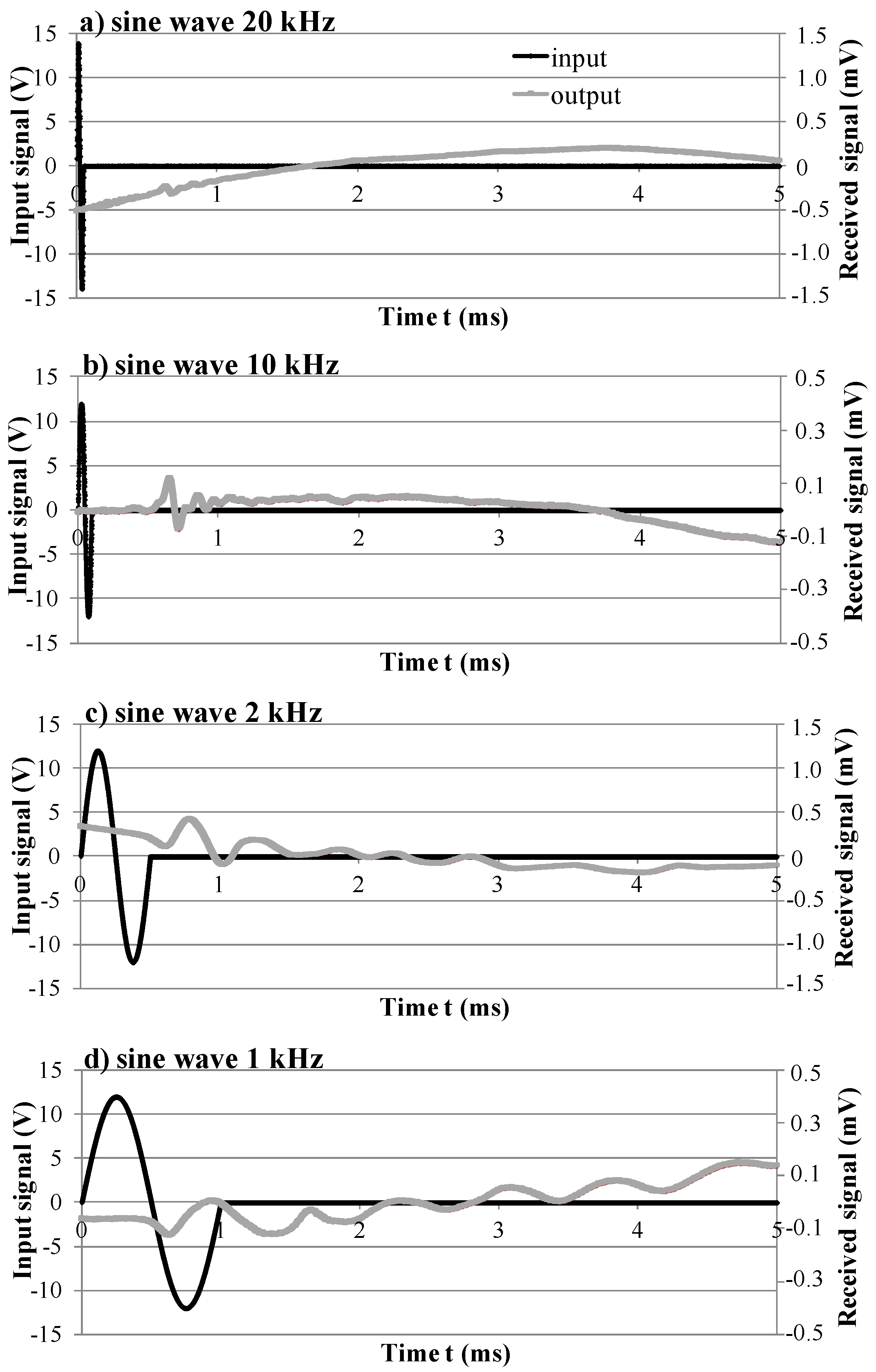
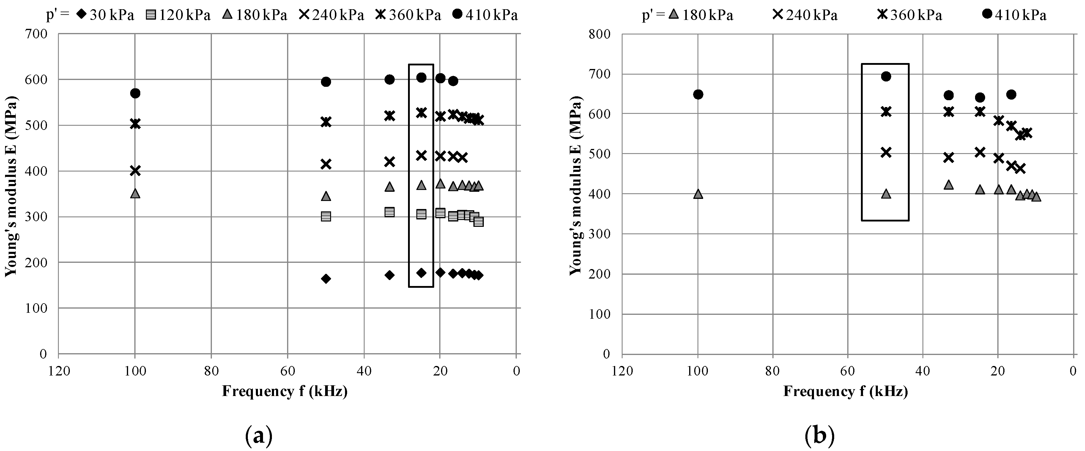
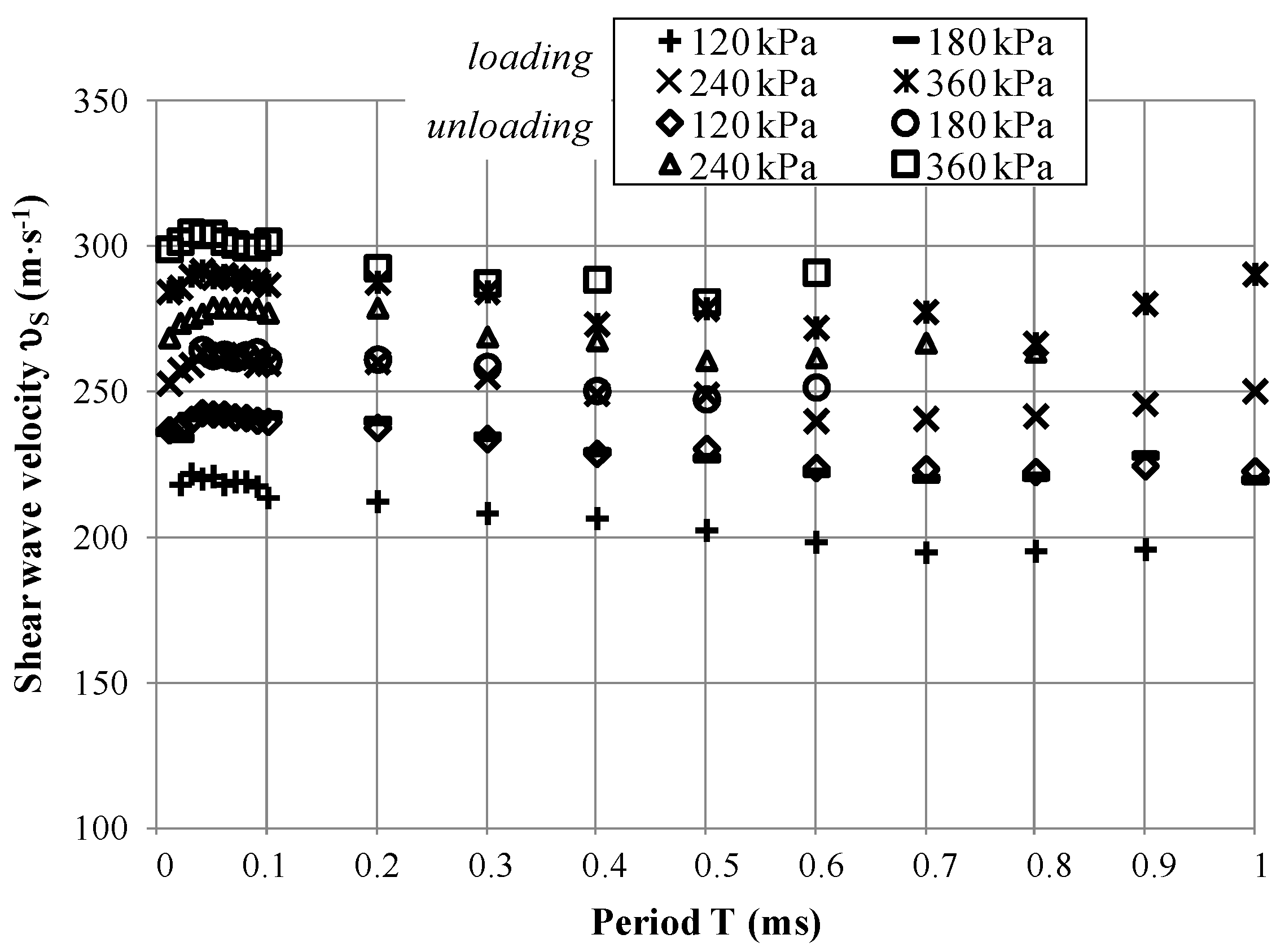
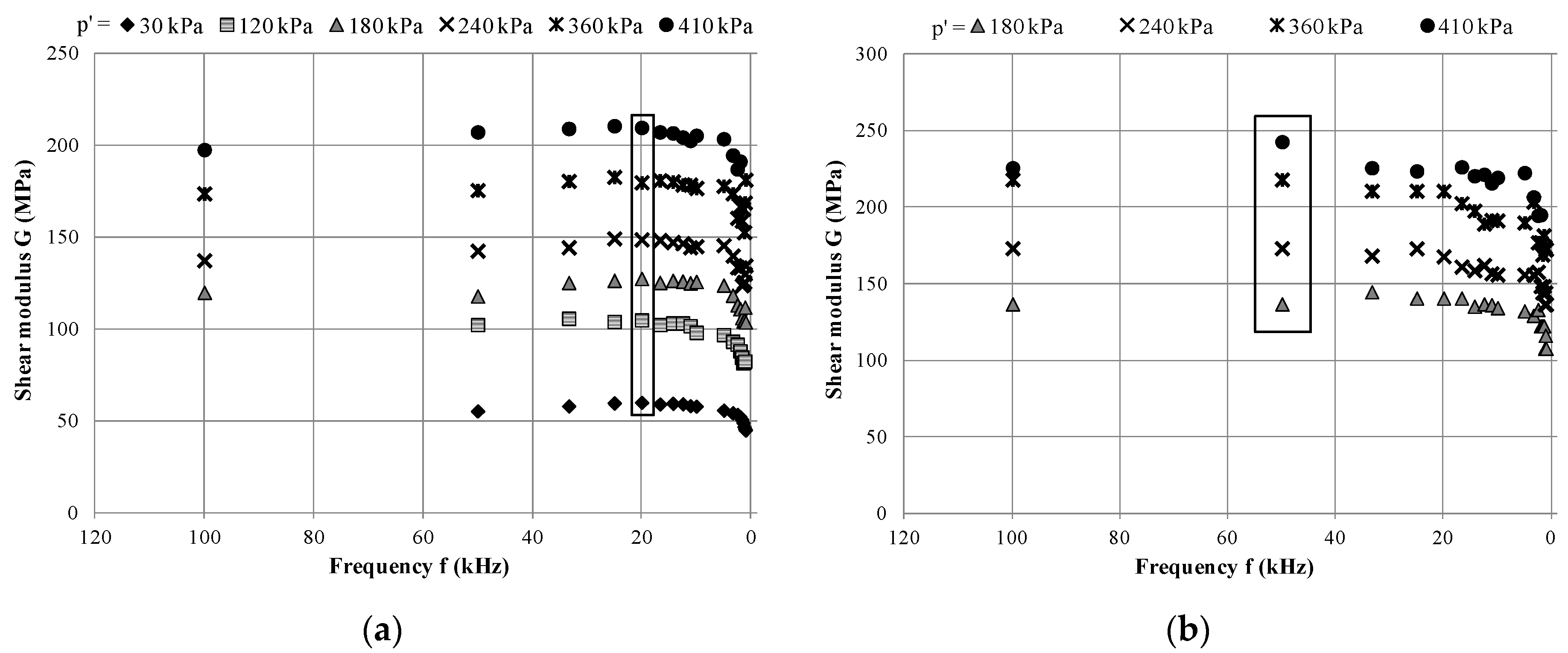
3.1. Frequency Dependency

In Figure 8 and Figure 9, the variation of the measured shear wave velocity (υS) with a predetermined period of propagating wave at different specified stress levels is shown. In Figure 10, however, the equivalent plot for measured compression wave velocity (υP) is illustrated. The presented results are related to both procedures adopted for determining the travel time.
Figure 8. Variation of measured υS with period: peak-to-peak method. (a) Period’s range from 0 to 1 ms; (b) Period’s range from 0.01 to 0.1 ms.
Applsci 06 00049 g008
Inspection of Figure 8 and Figure 9 indicates that, regardless of the method used to measure the travel time, the shear wave velocities decrease with the predetermined period (T), which transfers to frequency (f). Oscillation frequency is in fact the inverse of period. The linear approximation fits accurately most of the presented data obtained using the peak-to-peak and start-to-start methods. The coefficient of determination (R2) reaches high values, from 70% upwards, which shows that for the studied cohesive material, the linear regression functions explain the majority of υS variation. In general, the differences in the shear wave velocities with different frequencies are not large, from 18 to 27 m·s−1 and from 32 to 38 m·s−1, depending on the technique used to measure the travel time.
Figure 9. Variation of measured υS with period: start-to-start method. (a) Period’s range from 0 to 1 ms; (b) Period’s range from 0.01 to 0.1 ms.
Applsci 06 00049 g009
Figure 10. Variation of measured υP with period. (a) Peak-to-peak method; (b) start-to-start method.
Applsci 06 00049 g010
In said graphs, the influence of stress level (p’) is visible, as well. The average effective stress level significantly affects υS. For the highest pre-set pressure, i.e., 410 kPa, the authors received the highest values of shear wave velocity, with average values around 307 m·s−1 (peak-to-peak method) and 319 m·s−1 (start-to-start method). The lowest values of νS were recorded for the smallest given stress (30 or 180 kPa), their average being around 160 m·s−1 (peak-to-peak method) and 246 m·s−1 (start-to-start method). The difference in υS decreases with the increasing pressure value.
The results of the current study show also that for the period of propagation lasting up to 0.1 ms (i.e., f = 10 kHz), both selected procedures used in the time domain methods consistently produce the values of υS, which are less dependent on frequency than in the case of a larger period of wave (Figure 8 and Figure 9 on the right). The frame in these figures indicates the highest values of shear wave velocity for each mean effective stress level. The authors suggest in this way certain frequencies at which the bender elements tests should be performed. Hence, the recommended frequency values, for which the highest shear wave velocities can be obtained, are in the range of 20 to 50 kHz. Certainly, it should be remembered that the optimum frequency of excitation depends on many factors, for example on the pressure applied in the cell during tests [46]. There is no rule at all for choosing the best wave [47]. In the literature, some authors have reported their experience with choosing a specific frequency. Brignoli et al. in 1996 [38] noted that when bender elements are measuring the samples, whose height is between 100 and 140 mm, the most interpretable output waves occur in the range from 3 to 10 kHz. Jovočič et al. [33], however, observed that with a higher frequency, the near field effect is less discernible. For stiffer materials, the required frequency must be higher than the reported 10 kHz [33], although the problem of overshooting becomes more important. In addition to this, a high frequency wave attenuates faster than the low frequency one, provided the medium is the same. The fact that the use of a high frequency gives the clearest output signals remains undisputed.
In the case of compression waves (Figure 10), the authors carried out research in the frequency scope of up to 10 kHz. A very large dispersion of the results and a lack of dependence of υP on the frequency ratio, as well as on mean effective stress can be clearly noticed. The authors could not find a proper relationship of υP vs. frequency and mean effective stress. Empirical equations expressing the variation of P-wave velocity with frequency are characterized, however, by the low coefficients of determination (R2), listed in Figure 10. In general, the differences in compression wave velocities with the different frequencies reach high values, from 54 to 110 m·s−1 and from 19 to 57 m·s−1, depending on the technique used to measure the travel time.
In Figure 11 and Figure 12, the effect of excitation frequency on shear modulus (Figure 11) and Young’s modulus (Figure 12) is presented. The excitation frequencies varied from 1 to 100 kHz. The specimens were subjected to various isotropic effective confining pressures. It was observed (black frame in the figures) that the best signal, and consequently the greatest values of shear modulus (G), were received at the excitation frequency, whose values were equal 20 kHz for the peak-to-peak method (Figure 11a) and 50 kHz for the start-to-start method (Figure 11b). The excitation frequency being equal to (Figure 12b) or smaller than 50 kHz (Figure 12a) gave the greatest values of Young’s modulus (E), as well. It is worth paying attention to a decrease in the modulus values along with the decreasing frequency, although Gmax and Emax values were not obtained for the highest frequency, as already mentioned above. The average Gmax value obtained from all applied values of pressure ranged from 139 MPa to 194 MPa, depending on the measurement of the travel time, while average Emax was around 405 MPa and 557 MPa. In the case of the minimal dynamic properties of the studied soils, using the lowest frequencies resulted in the smallest values of G and E, with the average minimal G ranging from 116 MPa to 152 MPa and the minimal E ranging from 379 MPa to 509 MPa.
Figure 11. Variation of dynamic stiffness with frequency. (a) Peak-to-peak method; (b) start-to-start method.
Applsci 06 00049 g011
It should be also pointed out that the values of E are arranged in some trend with increasing frequency, whereas the values of υP do not show any dependence on frequency. This may seem incorrect, because Young’s modulus is relevant to the compression wave velocity, due to the motion of the particles. However, it must be remembered that the authors used the results of υP only indirectly, in order to determine the proper value of ν.
Figure 12. Variation of Young’s modulus with frequency. (a) Peak-to-peak method; (b) start-to-start method.
Applsci 06 00049 g012

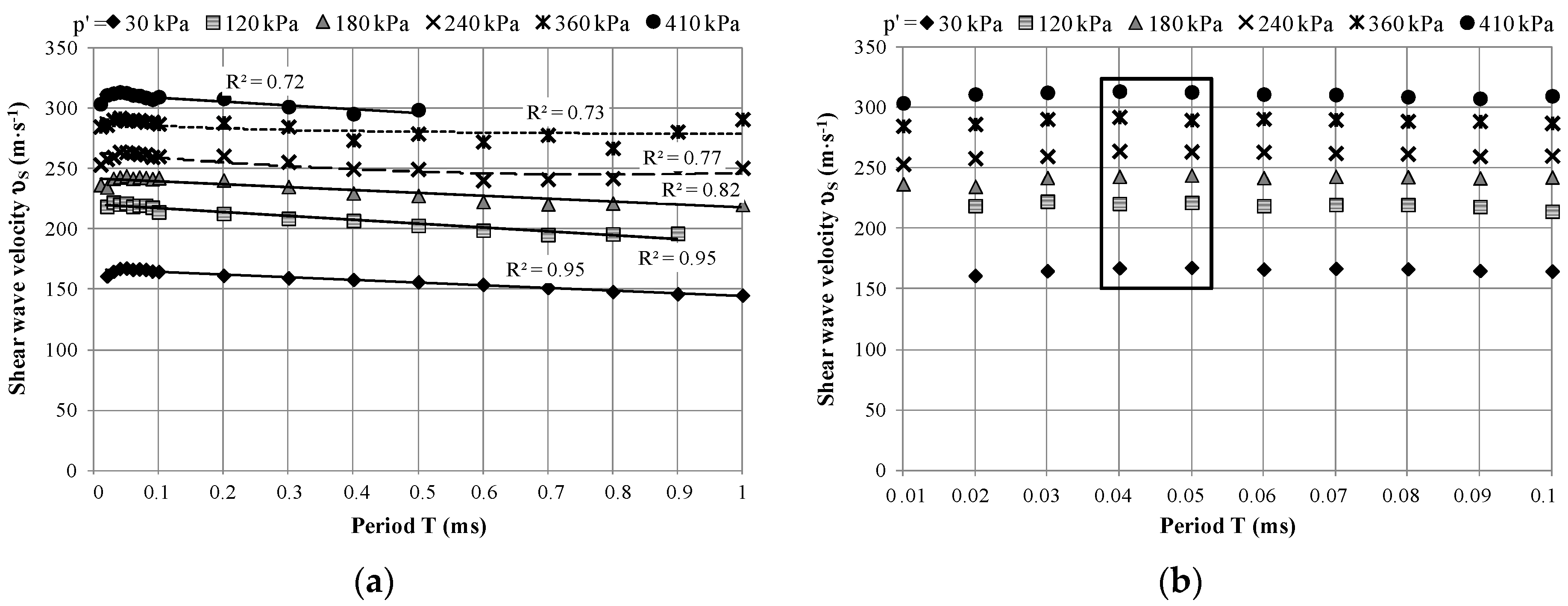
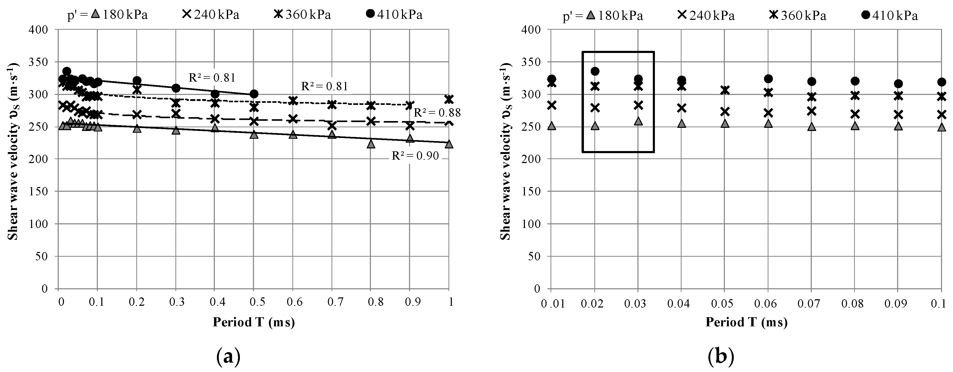
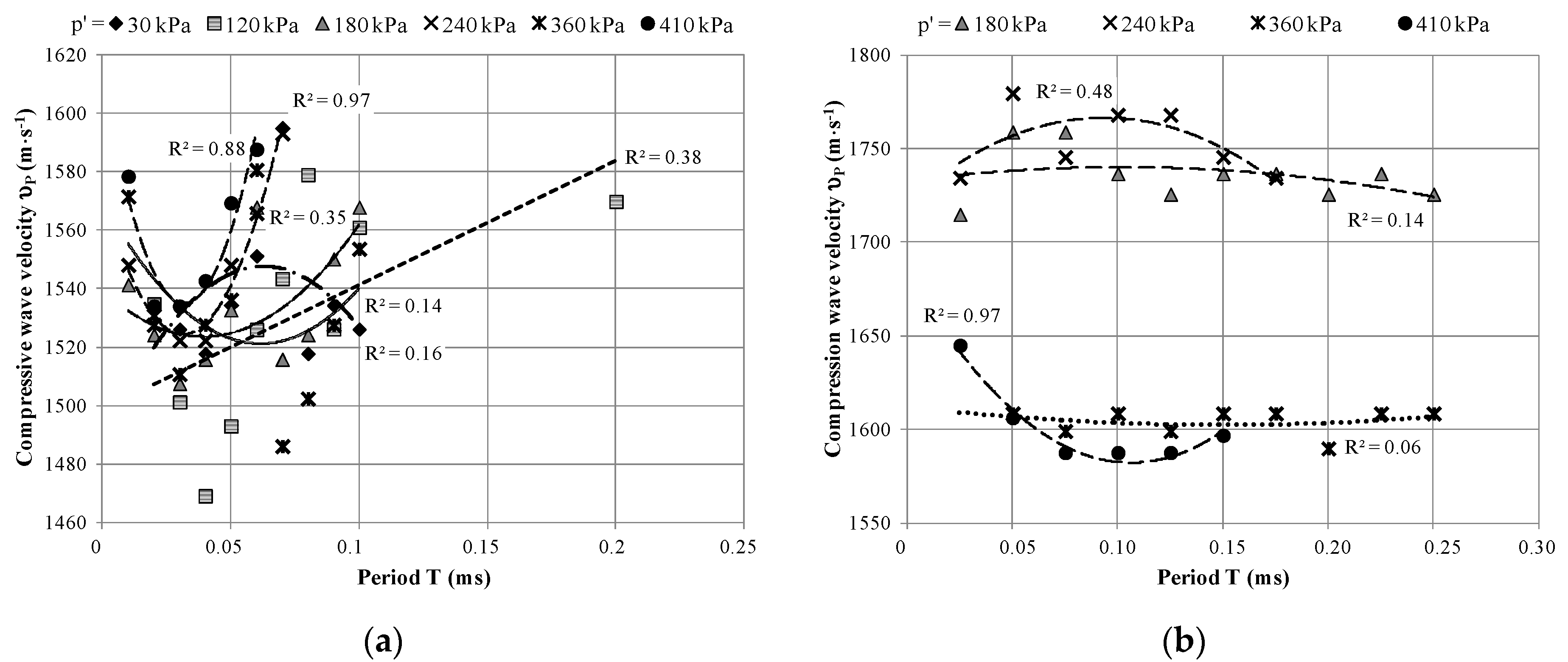
3.2. The Effect of Stress Level

In Table 2, the authors compiled the range of received S-wave and P-wave velocities after each consolidation stage. On the basis of Table 2, it can be concluded that the values of shear wave velocity obviously increase with applied pressure. At the same time, it is visible that the differences between the shear wave velocity values and each p’ amount to 20 to 30 m·s−1. The values of compression wave velocity confirmed the earlier observation about the lack of dependence between υP and stress level. The typical P-wave velocity of the tested material reached the value of 1400 to 1500 m·s−1 for the peak-to-peak method and 1600 to 1700 m·s−1 for the start-to-start method.
Table 2. Seismic waves velocities for various mean effective stress levels. (a) Peak-to-peak method; (b) start-to-start method.
(a)
(a)
Mean Effective StressS-Wave VelocityP-Wave VelocityAverage Ratio of Seismic Waves Velocities
p’ (kPa)υS (m·s−1)υP (m·s−1)υPS (-)
30145–1681518–15959.3
120195–2221469–15797.0
180221–2241508–15686.4
240240–2641522–15935.9
360267–2921486–15815.3
410296–3141435–15885.0
(b)
(b)
Mean Effective StressS-Wave VelocityP-Wave VelocityAverage Ratio of Seismic Waves Velocities
p’ (kPa)υS (m·s−1)υP (m·s−1)υPS (-)
180224–2601715–17596.8
240252–2841734–17796.3
360281–3191590–16094.7
410301–3361588–16454.9
In Table 2, additionally, the average ratio list of seismic wave’s velocities is enclosed. It is evident that the values of υP are several times higher, when compared with υS. The υPS velocity ratio has the variation interval ranging from 5.0 to 9.3. The authors obtained larger values of P-wave velocity than is observed in certain positions in the literature. Das and Ramana [48], for example, reported the characteristic compression wave velocity as ranging from 1220 m·s−1 to 1370 m·s−1 for saturated clay, although the ratio υPS was in the range of 8.0 to 9.0, thus similar to those obtained by the authors. Gary Mavko [49], on the other hand, in his study on Parameters That Influence Seismic Velocity mentions P-wave velocity for saturated clays as being in the range of 1100 to 2500 m·s−1. Campanella and Steward [50] detailed typical speeds of longitudinal and transversal waves to a depth of 40 m. According to their research, compressive wave velocity for saturated soils may have values between 1500 and 1900 m·s−1.
In Table 3, the results of the average dynamic Poisson’s ratio computed for each applied mean effective stress is shown. νd was determined on the basis of the relationship between S-wave and P-wave velocities (Equation (8)). The values of νd seem to be consistent with the literature [4,51,52]. The authors described the values of this parameter in another publication [23], in which the results obtained for saturated clay were at the level of 0.40 to 0.50, which is similar to the value obtained during the current studies. It is interesting to note that there is no significant change in νd regarding the pressure. Variation in Poisson’s ratio amounts to approximately 4% and approaches 0.5. Moreover, a number of different techniques for interpreting the BE results causes no definite difference in the values of Poisson’s ratio. Based on the experiments conducted, a general trend can be observed: as far as tested clayey material is concerned, Poisson’s ratios represent little appreciable change with regard to shear modulus (Figure 13). The values of νd were used afterwards in order to determine the dynamic modulus of elasticity (E).
Table 3. Dynamic Poisson’s ratio for various mean effective stress levels. (a) Peak-to-peak method; (b) start-to-start method.
(a)
(a)
Mean Effective StressAverage Dynamic Poisson’s Ratio
p’ (kPa)νd (-)
300.48
1200.47
1800.46
2400.46
3600.44
4100.44
(b)
(b)
Mean Effective StressAverage Dynamic Poisson’s Ratio
p’ (kPa)νd (-)
1800.47
2400.46
3600.44
4100.44
Figure 13. Shear modulus versus dynamic Poisson’s ratio. (a) Peak-to-peak method; (b) start-to-start method.
Applsci 06 00049 g013
The effect of mean effective stress on the small strain shear modulus and on the small strain modulus of elasticity of the examined silty clays is displayed in Figure 14 and Figure 15. The presented data were obtained for one excitation frequency, selected on the basis of its greatest values of dynamic properties regarding the analyzed soil specimens, as described in the previous section. BE measurements show that Gmax and Emax values increase with confining pressure as a linear function. Shear modulus at small strains, which was calculated for the tested material using Equation (6), does not exceed the interval of 60 to 242 MPa, regarding the travel time measurement. The modulus of elasticity at small strains, on the other hand, varies from 178 MPa to 694 MPa.
Figure 14. Elastic moduli from the peak-to-peak method under different stress levels.
Applsci 06 00049 g014
Figure 15. Elastic moduli from the start-to-start method under different stress levels.
Applsci 06 00049 g015

3.3. Comparison of Results from Different Methods

The input signals employed in all of the tests were single sinusoidal pulses with different frequencies, obtained using peak-to-peak and start-to-start methods. The amplitude of input signals in both cases was fixed at ±15 V. The tip-to-tip distances between the transducers were used to calculate the shear wave velocity of the samples (Equation (5)). All of the test traces were examined in the time domain, in order to obtain the travel time of the wave through the specimens.
In Figure 16, S-wave velocities determined by means of the two analyzed time domain techniques are portrayed. It is clearly visible that travel time derived from the start-to-start method must be longer due to the presence of the greatest values of the shear wave velocities. The difference in the obtained values of υS between these two methods remains at the average level of 21.25 m·s−1, in favor of the start-to-start method (Figure 17a). Naturally, these spotted differences vary, depending on the mean effective stress.
Figure 16. Comparison of υS obtained using various methods of travel time determination.
Applsci 06 00049 g016
In Figure 17b, the evolution of the shear stiffness modulus based on travel time deduced by means of the peak-to-peak and start-to-start techniques is summarized. In this comparison, the second of the aforementioned methods comes off as the better one. The average difference in stiffness of the examined cohesive material falls in the range of about 33.44 MPa. For the Emax (Figure 17c), the discrepancy between the results of two different interpretation methods achieves a maximum percentage of about 16% (89.2 MPa).
Figure 17. Comparison of results obtained by means of the peak-to-peak and start-to-start methods. (a) Shear wave velocity; (b) small strain shear modulus; (c) small strain Young’s modulus.
Applsci 06 00049 g017
In conclusion, it is worth noting that in the case of the start-to-start method, the findings of υS and Gmax lie on a straight line, but of a different gradient. This observation is not reflected in the outcomes regarding Emax. The results obtained with the use of the peak-to-peak method appear to be more scattered. On the basis of Figure 17, it can be noted that the S-S method (start-to-start method) of identification results in a relatively smaller variation, when compared to the P-P technique (peak-to-peak method). The latter method yields slightly smaller values of the dynamic parameters.

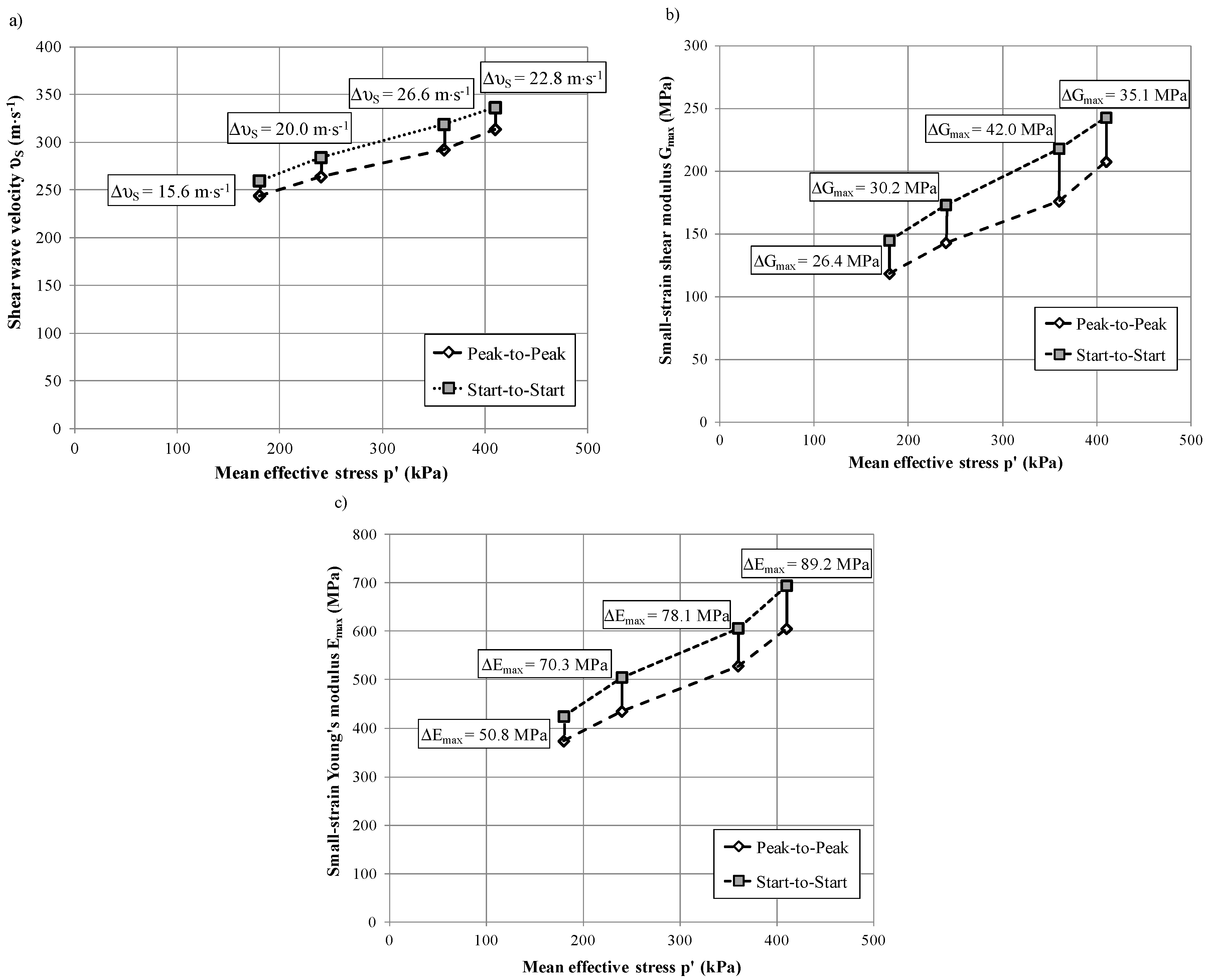
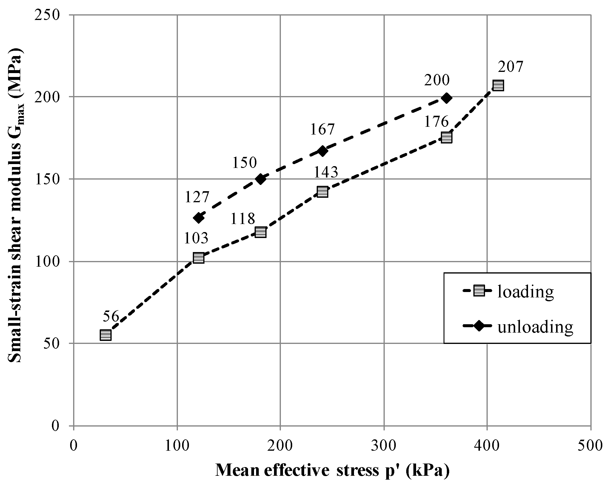
3.4. The Effect of Unloading

The aim of the current study, besides finding S-wave velocity and the small strain shear modulus when loading soil samples, was also to find υS and Gmax while unloading. The unloading process of the tested material was carried out to the pressure level of 120 kPa. In Figure 18 and Figure 19, the values of computed parameters from the loading and the subsequent unloading stages are presented.
During the inspection of Figure 18 and Figure 19, the authors noticed that υS, unloading and consequently Gmax, unloading carry greater values than υS, loading and Gmax, loading. The variance between silty clay dynamic stiffness during loading and unloading stages falls within the range between 16.8 and 22.8 MPa. The biggest difference was obtained for the mean effective stress equal to 180 kPa, the smallest one for p’ = 360 kPa. The unloading process causes the increase of the results from 8% to 16%. Thus, it should be highlighted that the unloading of soil considerably improves its stiffness.
Figure 18. Shear wave velocity versus period at the loading and unloading stage.
Applsci 06 00049 g018
Figure 19. Small strain shear modulus versus mean effective stress at the loading and unloading stage.
Applsci 06 00049 g019

4. Conclusions

In this study, the characterization of the dynamic properties of cohesive material, namely silty clays, was inspected. The conducted experiments included the dynamic tests in the GDS Resonant Column Apparatus equipped with bender elements. The authors aimed to verify the dynamic behavior of clayey soil in connection with wave propagation produced by piezoelectric transducers. Shear wave velocity is related to the shear modulus of soil. Consequently, the measurements of the S-wave velocity provided a convenient method for determining soil stiffness. Additionally, the calculation of the P-wave velocity and, subsequently, the dynamic Poisson’s ratio allowed for the examination of Young’s modulus with regard to the tested cohesive material.
The findings of this research, in line with the literature in relation to the methods of interpretation of bender element test results, indicate that, for tests with piezoelectric transducers installed in the resonant column apparatus on silty clays, both analyzed techniques used as a part of the time domain methods, i.e., peak-to-peak and start-to-start, yield similar results. They are also considered as the most comprehensive and appropriate methods to identify the travel time of the shear waves propagating through the sample. The authors, however, did not inspect any other methods, like the cross-correlation or π-point phase, but the velocities established by those methods are comparable to the findings from the resonant column measurements [25]. The dynamic parameters obtained by the start-to-start method were always slightly larger (up to about 20%) than those obtained using the peak-to-peak method. According to the authors, this is a consequence of the broadening of the excitation pulses after they are propagated through the sample. The lowest wavelength in the presented experiments was about 1.0 mm, which was at least 10-times bigger than the largest grain size of soil sample (that was less than or equal to 100 μm). In addition, no inhomogeneous pockets were found in the sample constitution after a destructive analysis of the material. In these conditions the macroscopic sample was expected to behave as a conducting media, and no enhanced scattering was expected at the grain boundaries. Since the studied sample was homogeneous, in terms of the wavelength, the difference between the results from the two discussed techniques can be explained by taking into account different wave velocities and different attenuations of the frequency components that constitute the excitation peaks. Although each excitation pulse used in the experiments was considered to have a well-defined frequency, in reality, the pulses are composed of a continuity of different frequencies with different amplitudes. This happens due to the finite size of the excitation pulse in the time domain, which adds additional frequencies to it. In the start-to-start method, the results were strongly influenced by the fastest travelling wave, while in the peak-to-peak method, the frequency component with the highest amplitude was the one considered. From the Figure 9 and Figure 10, it can be clearly noticed that the wave velocity from the S-S method had an almost flat dependency as a function of frequency; however, in the P-P method, it has a change of about 20% in the frequency range experimented. This suggests that, in the S-S method, the frequency component responsible for the excitation of the detector is independent of the frequency chosen for the excitation pulse (due to the unintentional frequencies present in the excitation pulse). In certain experimental circumstances, such as during the measurements of G, the peak-to-peak method led to more scattered results, which were probably connected to the interpretation of the findings made by the authors. It must be always kept in mind, that even when using the same identification method, reading points differed with the laboratory [22]. The scatter in the S-S method was definitely smaller in comparison to another method. Presented results show and confirm observations made by previous researchers [6,22], acknowledging the status of the start-to-start method as the most prevalent and consistent method for the determination of travel time.
With reference to the dependence of the dynamic behavior of clayey material on various factors, the following conclusions can be drawn:
  • The data show that the input signal frequency, in particular frequencies, which are below the level of T = 0.1 ms, does not significantly affect the stiffness values obtained by both adopted identification methods. The decrease in frequency results in greater dependence on frequency.
  • The best measurements of travel time for the tested soils were received at the frequencies of the input signal in the range of 50 to 20 kHz. In most of the considered cases, the greatest values of the dynamic parameters were obtained when the frequencies from this range were applied.
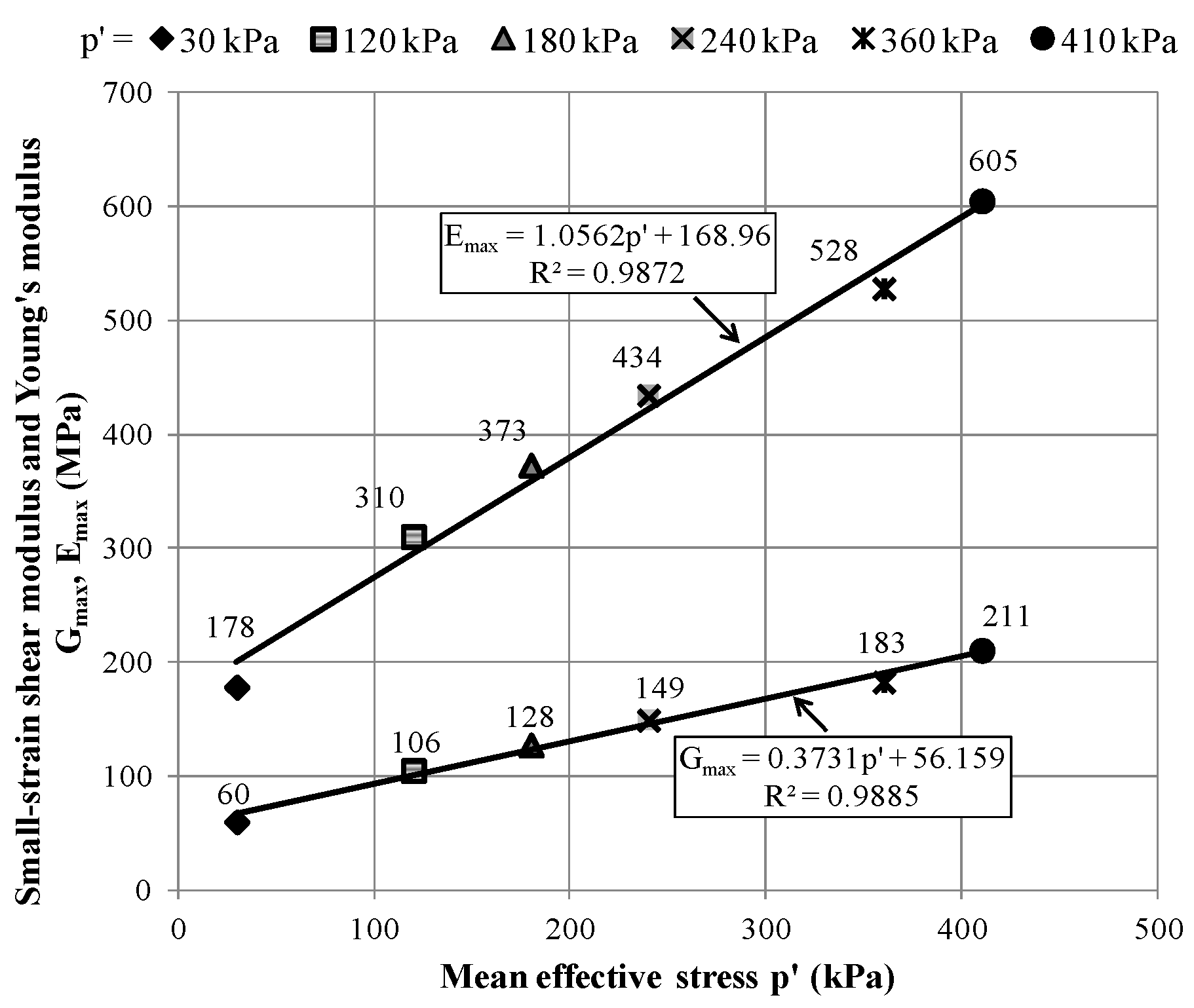
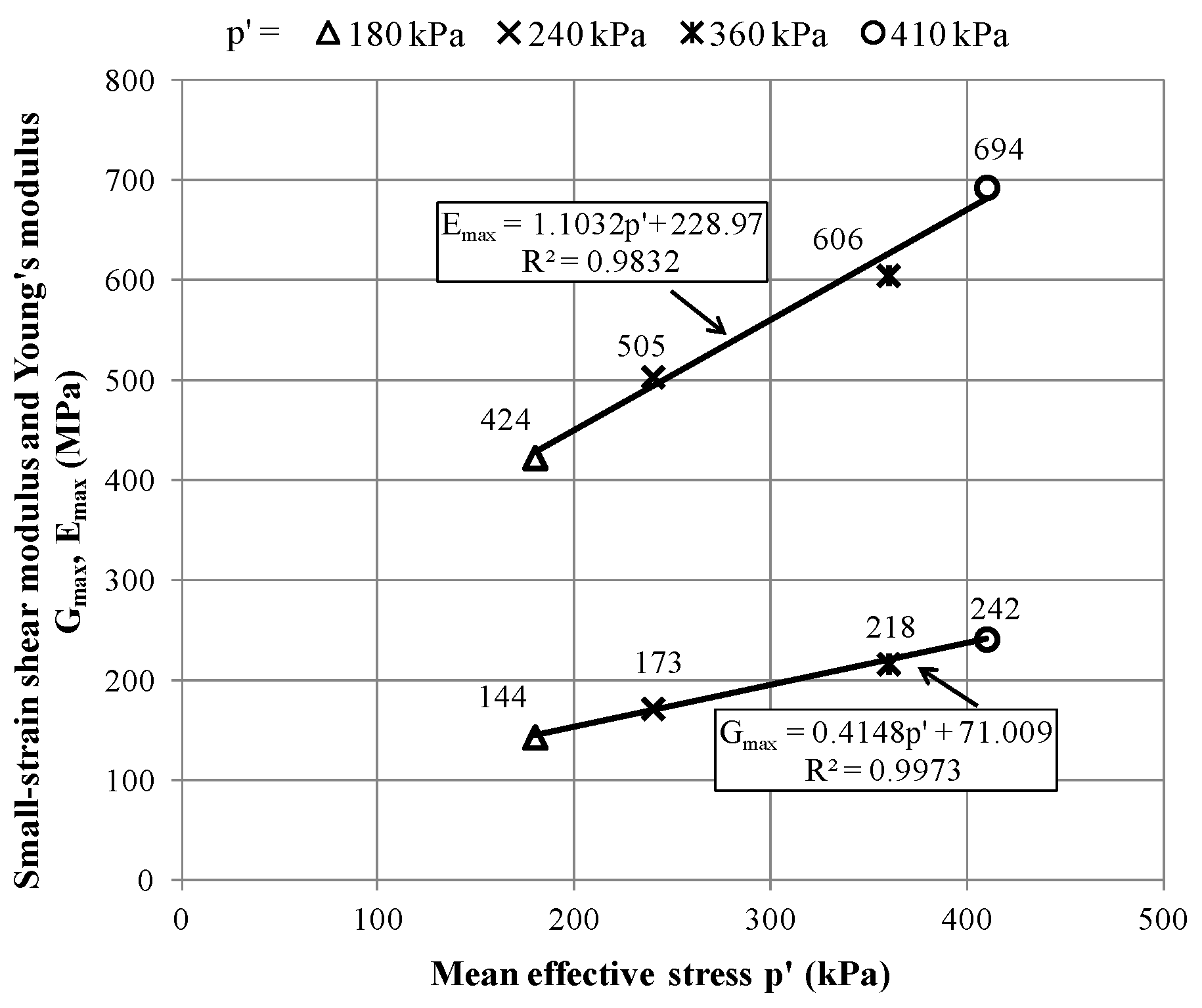
  • Mean effective stress has a visible influence on the seismic wave velocities and on the elastic modulus of the examined soils.
  • There are linear relationships between the mean effective stress and the small strain shear modulus and the small strain modulus of elasticity.
  • The compression waves propagate through the analyzed clayey material with far larger velocities than in the case of shear waves; at certain pressure levels, these velocities can be even up to 10-times larger.
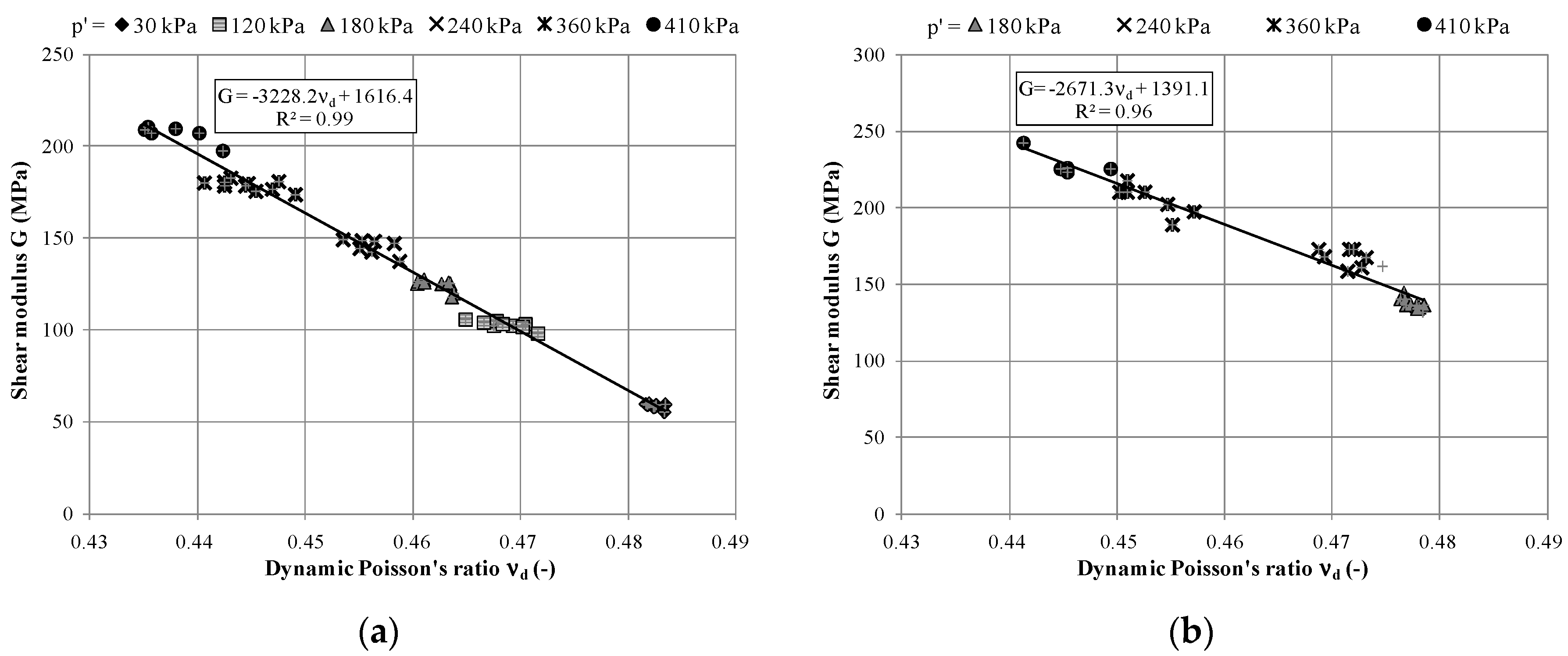
  • The dynamic Poisson’s ratio for the tested cohesive soils is almost constant, being approximately equal to 0.46.
  • The dynamic Poisson’s ratio linearly increases with the decrease of the shear modulus.
  • Concerning the unloading process, it profitably affects the stiffness of silty clays. The dynamic properties rise in their values, from 8% to 16%, owing to unloading.
Based on the results as described above, the standard procedure for the BE tests was proposed here in order to obtain appropriate test results in the present conditions. The authors discussed the important issue regarding the applied sciences, precisely the seismic research and dynamic response of porous material due to dynamic loads, such as earthquakes, traffic loads or machine vibrations. They attempted to characterize the dynamic properties of a fine-grained material, whose average porosity is approximately 0.44. This differs from the commonly-encountered in the literature dynamic characteristics of granular materials, non-cohesive soils, with a larger porosity value, described for example in [53,54]. The authors used generally-applied laboratory tests in order to investigate a still new material, as well as to expand the knowledge of the interpretation of this new material’s results.
The acquired knowledge of the behavior of the tested material should be verified in the process of modeling, using an appropriate model, such as the one proposed in [55].

Acknowledgments

The discussion about the results obtained was carried out with the valuable support of Bruno Cury Camargo (LNCMI—Laboratoire National des Champs Magnetiques Intenses, Toulouse, France).

Author Contributions

Wojciech Sas was the inventor of the research presented in this paper. Katarzyna Gabryś and Emil Soból conducted the described research and also performed geotechnical laboratory studies. Wojciech Sas and Katarzyna Gabryś prepared the manuscript. Katarzyna Gabryś and Emil Soból performed the analysis of the tests results. Alojzy Szymański consulted the research program and proofread the manuscript.

Conflicts of Interest

The authors declare no conflict of interest.

References

  1. Salacak, M.; Pinar, S.B.S. Soil parameters which can be determined with seismic velocities. Jeofizik 2012, 16, 17–29. [Google Scholar]
  2. Youn, J.-U.; Choo, Y.-W.; Kim, D.-S. Measurement of small-strain shear modulus Gmax of dry and saturated sands by bender element, resonant column, and torsional shear tests. Can. Geotech. J. 2008, 45, 1426–1438. [Google Scholar] [CrossRef]
  3. Burland, J.B.; Longworth, T.I.; Moore, J.F.A. Study of ground and progressive failure caused by deep excavation in Oxford clay. Géotechnique 1977, 27, 557–591. [Google Scholar] [CrossRef]
  4. Oshaki, Y.; Iwasaki, R. On dynamic shear moduli and Poisson’s ratio of soil deposits. Soils Found. 1973, 13, 61–73. [Google Scholar]
  5. Sas, W.; Głuchowski, A.; Radziemska, M.; Dzięcioł, J.; Szymański, A. Environmental and Geotechnical Assessment of the Steel Slags as a Material for Road Structure. Materials 2015, 8, 4857–4875. [Google Scholar] [CrossRef]
  6. Yamashita, S.; Kawaguchi, T.; Nakata, Y.; Mikami, T.; Fujiwara, T.; Shibuya, S. Interpretation of international parallel test on the measurement of Gmax using bender elements. Soils Found. 2009, 49, 631–650. [Google Scholar] [CrossRef]
  7. Benz, T. Small-Strain Stiffness of Soils and Its Numerical Consequences; Universität Stuttgart: Stuttgart, Germany, 2007. [Google Scholar]
  8. Menzies, B. Near-surface site characterization by ground stiffness profiling using surface wave geophysics. In H. C. Verma Commemorative Volume; Indian Geotechnical Society: New Delhi, Indian, 2000; pp. 1–14. [Google Scholar]
  9. Leong, E.C.; Cahyadi, J.; Rahardjo, H. Measuring shear and compression wave velocities of soil using bender-extender elements. Can. Geotech. J. 2009, 46, 792–812. [Google Scholar] [CrossRef]
  10. Ha Giang, P.H.; van Impe, P.; van Impe, W.F.; Menge, P.; Haegeman, W. Effects of grain size distribution on the initial small strain shear modulus of calcareous sand. In Proceedings of the 16th ECSMGE Geotechnical Engineering for Infrastructure and Development, Edinburg, UK, 13–17 September 2015; pp. 3177–3182.
  11. Sas, W.; Gabryś, K.; Szymański, A. Laboratoryjne badanie sztywności gruntu według Eurokodu 7 [In Polish] Laboratory tests of soil stiffness by Eurocode 7. Acta Sci. Pol. Ser. Archit. 2013, 12, 39–50. [Google Scholar]
  12. Sas, W.; Gabryś, K.; Szymański, A. Comparison of resonant column and Bender elements tests on selected cohesive soil from Warsaw. Electron. J. Pol. Agric. Univ. EJPAU 2014, 17, #07. Available online: http://www.ejpau.media.pl/volume17/issue3/art-07.html (accessed on 23 July 2014). [Google Scholar]
  13. Lawrence, F.V. Propagation of Ultrasonic Waves through Sand; Research Report R63-08; Massachusetts Institute of Technology: Cambridge, MA, USA, 1963. [Google Scholar]
  14. Lawrence, F.V. Ultrasonic Shear Wave Velocity in Sand and Clay; Research Report R65-05; Massachusetts Institute of Technology: Cambridge, MA, USA, 1965. [Google Scholar]
  15. Shirley, D.J. An improved shear wave transducer. J. Acoust. Soc. Am. 1978, 63, 1643–1645. [Google Scholar] [CrossRef]
  16. Dyvik, R.; Madshus, C. Lab Measurement of Gmax Using Bender Elements; Norwegian Geotechnical Institute: Oslo, Norway, 1985; pp. 186–196. [Google Scholar]
  17. Styler, M.A.; Howie, J.A. Continuous Monitoring of Bender Element Shear Wave Velocities During Triaxial Testing. Geotech. Test. J. 2014, 37, 218–230. [Google Scholar] [CrossRef]
  18. Ferreira, C.; Martins, J.P.; Correia, A.G. Determination of the small-strain stiffness of hard soils by means of bender elements and accelerometers. In Proceedings of the 15th European Conference on Soil Mechanics and Geotechnical Engineering; Athens, Greece, 12–15 September 2013, Andreas, A., Michael, P., Christos, T., Eds.; IOS Press: Amsterdam, The Netherlands, 2011; Volume 1, pp. 179–184. [Google Scholar]
  19. Viggiani, G.; Atkinson, J.H. Interpretation of bender element tests. Géotechnique 1995, 45, 149–154. [Google Scholar] [CrossRef]
  20. Lee, J.S.; Santamarina, J.C. Bender elements: Performance and signal interpretation. J. Geotech. Geoenviron. Eng. ASCE 2005, 131, 1063–1070. [Google Scholar] [CrossRef]
  21. Leong, E.C.; Yeo, S.H.; Rahardjo, H. Measuring shear wave velocity using bender elements. Geotech. Test. J. 2005, 28, 488–498. [Google Scholar]
  22. Camacho-Tauta, J.F.; Cascante, G.; da Fonseca, A.V.; Santos, J.A. Time and frequency domain evaluation of bender element systems. Géotechnique 2015, 65, 548–562. [Google Scholar] [CrossRef]
  23. Sas, W.; Gabryś, K.; Szymański, A. Determination of Poisson’s ratio by means of resonant column tests. Electron. J. Pol. Agricu. Univ. EJPAU 2013, 16, #03. Available online: http://www.ejpau.media.pl/volume16/issue3/art-03.html (accessed on 20 August 2013). [Google Scholar]
  24. Sas, W.; Gabryś, K. Laboratory measurement of shear stiffness in resonant column apparatus. ACTA Sci. Pol. Ser. Arch. 2012, 11, 29–39. [Google Scholar]
  25. Gabryś, K.; Sas, W.; Soból, E. Small-strain dynamic characterization of clayey soil from Warsaw. ACTA Sci. Pol. Ser. Arch. 2015, 14, 55–65. [Google Scholar]
  26. GDS Instruments Ltd. Bender Elements. In The GDS Bender Elements System Hardware Handbook for Vertical and Horizontal Elements; GDS Instruments Ltd.: Hampshire, UK, 2005. [Google Scholar]
  27. Cheng, Z.; Leong, E.C. A Hybrid Bender Element-Ultrasonic System for Measurement of Wave Velocity in Soils. Geotech. Test. J. 2014, 37, 377–388. [Google Scholar] [CrossRef]
  28. Chan, C.M. Bender Element Test in Soil Specimens: Identifying the Shear Wave Arrival Time. EJGE 2010, 15, 1263–1276. [Google Scholar]
  29. Clayton, C.R.I.; Theron, M.; Best, A.I. The measurement of vertical shear-wave velocity using side-mounted bender elements in the triaxial apparatus. Géotechnique 2004, 54, 495–498. [Google Scholar] [CrossRef]
  30. Brocanelli, D.; Rinaldi, V. Measurement of low-strain material damping and wave velocity with bender elements in the frequency domain. Can. Geotech. J. 1998, 35, 1032–1040. [Google Scholar] [CrossRef]
  31. Arroyo, M.; Greening, P.; Wood, D.M. An estimate of uncertainty in current pulse test practice. Riv. Ital. Geotec. 2001, 37, 17–35. [Google Scholar]
  32. Mitaritonna, G.; Amorosi, A.; Cotecchia, F. Multidirectional bender element measurements in the triaxial cell: Equipment set-up and signal interpretation. Riv. Ital. Geotec. 2010, 1, 50–69. [Google Scholar]
  33. Jovičić, V.; Coop, M.R.; Simic, M. Objective criteria for determining Gmax from bender element tests. Géotechnique 1996, 46, 357–362. [Google Scholar] [CrossRef]
  34. Polish Committee for Standardization. Geotechnical Investigations—Soil Classification—Part 2: Classification Rules; PN–EN ISO 14688-2:2004; Polish Committee for Standardization: Warsaw, Poland, 2004. (In Polish) [Google Scholar]
  35. Sas, W.; Gabryś, K.; Szymański, A. Effect of time on dynamic shear modulus of selected cohesive soil of one section of Express Way No S2 in Warsaw. Acta Geophys. 2015, 63, 398–413. [Google Scholar] [CrossRef]
  36. Head, K.H. Manual of Soil Laboratory Testing. Volume 3 Effective Stress Tests; J. Wiley & Sons Ltd.: New York, NY, USA, 1998. [Google Scholar]
  37. Viggiani, G. Panellist discussion: Recent advances in the interpretation of bender element tests. In Pre-Failure Deformation of Geomaterials; Satoru, S., Toshiyuki, M., Seiichi, M., Eds.; Balkema: Rotterdam, The Netherland, 1995; Volume 2, pp. 1099–1104. [Google Scholar]
  38. Brignoli, E.; Gotti, M.; Stokoe, K.H., II. Measurement of shear waves in laboratory specimens by means of piezoelectric transducers. ASTM Geotech. Test. J. 1996, 19, 384–397. [Google Scholar]
  39. Kawaguchi, T.; Mitachi, T.; Shibuya, S. Evaluation of shear wave travel time in laboratory bender element test. In Proceedings of 15th International Conference on Soil Mechanics and Geotechnical Engineering, Istambul, Turkey, 28–31 August 2001; Volume 1, pp. 155–158.
  40. Leong, E.C.; Yeo, S.H.; Rahardjo, H. Measuring Shear Wave Velocity Using Bender Elements. Geotech. Test. J. 2003. [Google Scholar] [CrossRef]
  41. Hasan, A.M.; Wheeler, S.J. Measuring travel time in bender/extender element tests. In Proceedings of the 16th ECSMGE Geotechnical Engineering for Infrastructure and Development, Edinburg, UK, 13–17 September 2015; pp. 3171–3176.
  42. Choo, H.; Larrahondo, J.; Burns, S.E. Coating Effects of Nano-Sized Particles onto Sand Surfaces: Small Strain Stiffness and Contact Mode of Iron Oxide-Coated Sands. J. Geotech. Geoenviron. Eng. 2015, 141, 04014077:1–04014077:10. [Google Scholar] [CrossRef]
  43. Lee, C.-J.; Hung, W.-Y.; Tsai, C.-H.; Chen, T.; Tu, Y.; Huang, C.-C. Shear wave velocity measurements and soil-pile system identifications in dynamic centrifuge tests. Bull. Earthq. Eng. 2014, 12, 717–734. [Google Scholar] [CrossRef]
  44. Fedrizzi, F.; Raviolo, P.L.; Vigano, A. Resonant column and cyclic torsional shear experiments on soils of the Trentino valleys. In Proceedings of the 16th ECSMGE Geotechnical Engineering for Infrastructure and Development, Edinburg, UK, 13–17 September 2015; pp. 3437–3442.
  45. Gabryś, K.; Szymański, A. Badania parametrów odkształceniowych gruntów spoistych w kolumnie rezonansowej [In Polish] Research of deformation parameters of cohesive soils in resonant column. Inżynieria Morska i Geotech. 2012, 4, 324–327. [Google Scholar]
  46. Amat, A.S. Elastic Stiffness Moduli of Huston Sand. Master’s Thesis, University of Bristol, Bristol, UK, 2007. [Google Scholar]
  47. Ali, H.; Mahbaz, S.B.; Cascante, G.; Garbinsky, M. Low strain measurement of shear modulus with resonant column and bender element tests—Frequency effects. In Proceedings of the GeoMontreal 2013: Geoscience for Sustainability, Montreal, QC, Canada, 29 September–3 October 2013.
  48. Das, B.M.; Ramana, G.V. Principles of Soil Dynamics, 2nd ed.United States of America: Stamford, CT, USA, 2011.
  49. Mavko, G. Parameters that Influence Seismic Velocity. Conceptual Overview of Rock and Fluid Factors that Impact Seismic Velocity and Impedance; Stanford Rock Physics Laboratory: Standford, CA, USA, 2009. [Google Scholar]
  50. Campanella, R.G.; Stewart, W.P. Seismic cone analysis using digital signal processing for dynamic site characterization. Can. Geotech. J. 1992, 29, 477–486. [Google Scholar] [CrossRef]
  51. Poisson’s ratio. Available online: http://www.engineeringtoolbox.com (accessed on 21 September 2015).
  52. Otsubo, M.; O’Sullivan, C.; Sim, W.W.; Ibraim, E. Quantitative assessment of the influence of surface roughness on soil stiffness. Géotechnique 2015, 65, 694–700. [Google Scholar] [CrossRef]
  53. Wichtmann, T.; Triantafyllidis, T. Stiffness and Damping of Clean Quartz Sand with Various Grain-Size Distribution Curves. J. Geotech. Geoenviron. Eng. 2014, 140, 06013003:1–06013003:4. [Google Scholar] [CrossRef]
  54. Qiu, T.; Huang, Y.; Guadalupe-Torres, Y.; Baxter, C.D.P.; Fox, P.J. Effective Soil Density for Small-Strain Shear Waves in Saturated Granular Materials. J. Geotech. Geoenviron. Eng. 2015, 141, 04015036:1–04015036:11. [Google Scholar] [CrossRef]
  55. Aggelis, D.G.; Tsinopoulos, S.V.; Polyzos, D. An iterative effective medium approximation (IEMA) for wave dispersion and attenuation predictions in particulate composites, suspensions and emulsions. J. Acoust. Soc. Am. 2004, 116, 3443–3452. [Google Scholar] [CrossRef] [PubMed]

