Vehicle Speed Estimation and Forecasting Methods Based on Cellular Floating Vehicle Data

Abstract

Traffic information estimation and forecasting methods based on cellular floating vehicle data (CFVD) are proposed to analyze the signals (e.g., handovers (HOs), call arrivals (CAs), normal location updates (NLUs) and periodic location updates (PLUs)) from cellular networks. For traffic information estimation, analytic models are proposed to estimate the traffic flow in accordance with the amounts of HOs and NLUs and to estimate the traffic density in accordance with the amounts of CAs and PLUs. Then, the vehicle speeds can be estimated in accordance with the estimated traffic flows and estimated traffic densities. For vehicle speed forecasting, a back-propagation neural network algorithm is considered to predict the future vehicle speed in accordance with the current traffic information (i.e., the estimated vehicle speeds from CFVD). In the experimental environment, this study adopted the practical traffic information (i.e., traffic flow and vehicle speed) from Taiwan Area National Freeway Bureau as the input characteristics of the traffic simulation program and referred to the mobile station (MS) communication behaviors from Chunghwa Telecom to simulate the traffic information and communication records. The experimental results illustrated that the average accuracy of the vehicle speed forecasting method is 95.72%. Therefore, the proposed methods based on CFVD are suitable for an intelligent transportation system.

1. Introduction

In recent years, the usage and improvement of mobile techniques have been growing for a variety of real-life applications. For instance, many intelligent transportation systems (ITSs) and services have been designed and developed by several enterprises [1,2,3,4]. For the development of ITSs, studying how to collect the traffic information efficiently is a really important topic. The case studies of cooperative intelligent transportation systems (C-ITS) [2,3] and connected-vehicle technology [4] developed real-time traffic information collection methods and evaluated traffic status. Furthermore, Gao et al. [1] considered traffic status to predict travel time for the design of a navigation system and the avoidance of traffic jams.

ITSs have three kinds of popular position collection approaches, which are the vehicle detector (VD), the reports of global positioning system (GPS)-equipped probe cars and cellular floating vehicle data (CFVD). VD is a sensor based on the techniques of active infrared/laser, magnetic, radar or video to regularly detect vehicles on a road for the analysis of time mean speed and traffic flow [5,6] GPS-equipped probe cars can periodically report their location information to a server for computing the space mean speed [7]. CFVD, which is obtained by tracking the network signals of the mobile station (MS) in the car, can be analyzed to estimate the traffic information (e.g., traffic flow, vehicle speed and traffic density) [5]. The advantages and limitations of these three methods are illustrated in the following paragraphs.

The establishment cost and maintenance fees of VDs were discussed and analyzed in some studies from different countries [8]. For instance, the Texas Transportation Institute spent 43,500 U.S. dollars to install video image vehicle detection systems (VIVD) for the detection of real-time traffic information in 2002. The Ministry of Transportation and Communications in Taiwan spent 75,873 U.S. dollars to establish one VD per each kilometer on Taiwan Highway No. 1 for the collection of real-time road information [9]. However, the maintenance fees of VD solutions are really high because the damage of VD usually result by the environmental factors.

Some studies discussed traffic collection and estimation methods based on the reports of GPS-equipped probe cars, which were compared to the traffic information from VDs for the evaluation of traffic estimation accuracies. For instance, Cheu et al. [10] showed that the lower error rate of space mean speed estimation (less than 3%) can be obtained with enough active probe vehicles. Herrera et al. [10] showed that GPS-equipped probe vehicles periodically recorded their speeds and locations in practical environments for traffic information estimation. Furthermore, their study suggested that a 2%–3% penetration of GPS-equipped probe vehicles is enough to provide accurate measurements of space mean speed. However, the cost of deployment of GPS-equipped probe cars is very expensive for reaching a penetration rate of 2%–3% [10,11].

CFVD can be obtained by tracking MS signals (call arrival (CA), handover (HO), double handover (DHO), normal location update (NLU) and period location update (PLU)), and it can be used for the analysis of traffic status [12,13]. Furthermore, the International Telecommunication Union (ITU) indicated that the handphone penetration rate is more than 100% in many countries [14], and the penetration rate is high enough to assume that everyone has a handphone. Therefore, some studies assumed one handphone in one vehicle. For instance, Lin et al. [9] analyzed two HO locations based on the location service (LCS) as CFVD to estimate the real-time travel time and real-time vehicle speed between HO locations. Their experimental results indicated that the accuracy of the proposed traffic information estimation method was high. However, due to tracing the routes of each MS, a higher computation power is required, and privacy threats may exist. Moreover, future traffic information forecasting based on CFVD has not been investigated.

Therefore, this study proposes analytic models and traffic information estimation methods based on CFVD to obtain a low-cost solution for ITS. The proposed analytic models are used to analyze the relationship between traffic information (e.g., traffic flow, traffic density and vehicle speed) and the amount of cellular network signals (e.g., HO, NLU, CA and PLU). Then, traffic information can be estimated based on the proposed analytic models and CFVD. Furthermore, a vehicle speed forecasting method based on a back-propagation neural network (BPNN) algorithm is proposed to analyze the estimated vehicle speeds from CFVD and to predict the future vehicle speed for road users.

The rest of this study is organized as follows. Section 2 discusses the related studies and techniques of traffic information estimation and forecasting methods. Section 3 purposes vehicle speed estimation and forecasting methods based on CFVD. A case study of a highway in Taiwan and experimental results are illustrated and analyzed in Section 4. Finally, Section 5 summarizes the contributions of this study and presents future work.

2. Literature Review

In this section, the techniques of cellular networks, CFVD and traffic information forecasting methods are illustrated in the following subsections. The architecture of cellular networks and mobility management methods are described in Section 2.1. Section 2.2 presents the advantages and limitations of each CFVD method. Finally, traffic information estimation and forecasting methods based on data mining techniques are discussed in Section 2.3.

2.1. Cellular Networks

This section presents the network architecture of the Global System for Mobile Communications (GSM)/General Packet Radio Service (GPRS)/Universal Mobile Telecommunications System (UMTS). The components and mobility management (MM) in cellular networks are described as follows.

2.1.1. System Components

The GSM consists of the MS, base transceiver station (BTS), base station controller (BSC), mobile switching center (MSC), home location register (HLR) and visitor location register (VLR). MSs communicate with the network through the BTS and BSC via the A-bis interface (the interface between the BTS and the BSC). The BSC communicates with the MSC via the A (the interface between the BSC and the circuit switched core network) interface, and MSC can connect the calls from the MSs to the public switched telephone network (PSTN). Moreover, the HLR and VLR can provide mobility management and record the location information of the MS [15].

GPRS evolved from GSM and added two new components, which include the serving GPRS support node (SGSN) and the gateway GPRS support node (GGSN). GPRS can establish the data connection with the Internet. However, this study focuses on circuit-switched networks, and the signaling of packet-switched networks is not discussed and analyzed.

The UMTS consists of user equipment (UE), Node B, the radio network controller (RNC) and the components in GSM and GPRS. UEs communicate with the network through Node B and the RNC via the Iub (the interface between the Node B and the RNC) interface. The BSC communicates with the MSC via the IuCS (the interface between the RNC and the circuit switched core network) interface, and the MSC can connect the calls from the UEs to the PSTN [15].

2.1.2. Mobility Management

For MM, the functions related to the management of the common transmission resources may be performed in accordance with the MS/UE. There are two modes, which include idle mode and radio resource (RR) connected mode in RR management.

Idle Mode

In idle mode, the location updating procedures are performed for MM. The location updating procedure is a general procedure, which is used for the following purposes [16].

(1)

Normal location updating: NLU is performed when a new location area is entered (European Telecommunications Standards Institute (ETSI), 1995).

(2)

Periodic location updating: PLU is performed at the expiration of the timer (ETSI, 1995).

(3)

International Mobile Subscriber Identity (IMSI) attach: IMSI attach is performed when the MS is turned on [16].

Radio Resource Connected Mode

In RR connected mode, the handover procedures are performed for MM. The MSC can control the call and the MM of the MS during the call. When MS enters a new cell during a call, the handover procedure is performed to provide good quality RR by the MSC [17]. This study assumes that each MS in the car can perform the handover procedure in accordance with the specification when the MS enters a new cell during a call.

2.2. Traffic Information Estimation Methods

The techniques of traffic information estimation method based on CFVD can be classified into two groups, which include (1) location services and (2) signal statistics.

2.2.1. Location Services

Several location positioning methods, which were defined in the LCS specification of the 3rd Generation Partnership Project (3GPP), could be grouped into three classes, including: (1) assisted GPS (A-GPS) methods; (2) mobile scan report (MSR)-based location methods; and (3) database lookup methods [18,19].

For A-GPS methods, a GPS component should be equipped in each MS to determine the location of the MS. However, these methods cannot be performed for the MSs without GPS components. Therefore, A-GPS methods are not discussed and applied in this study.

For MSR-based location methods, each MS can send periodically MSR messages (e.g., received signal strength indication (RSSI), round-trip delay and relative delay) to core networks in cellular networks (e.g., Global System Mobile Communications (GSM), Universal Mobile Telecommunications System (UMTS) and Long-Term Evolution (LTE)) [9]. Some studies analyzed the MSR messages to determine the locations of MSs, and these locations can be used to estimate traffic information. For instance, Cheng et al. [9] proposed a fingerprint-positioning algorithm (FPA) based on the k-nearest neighbors (kNN) algorithm to analyze the RSSIs of MSR messages for generating the locations of MS in car, and the average vehicle speed and travel time between two locations of the same MS can be estimated by FPA. Because the interfaces of A-bis and Iub in radio networks should be monitored to retrieve RSSIs for FPA, it is required to have above 10,000 servers to deploy to proceed with recording and analysis by Taiwanese environment. However, core network signals (e.g., CA, HO, NLU and PLU) can be captured via the interfaces of A and IuCS, so only less than 100 servers are needed to be deployed by the Taiwanese environment. The experiment results of FPA showed a high accuracy of vehicle speed estimation, although this method may need higher signaling costs for sending MSR message between MSs and base stations.

For database lookup methods, the information of cellular network signals, which include cell ID, CA, HO and NLU, are considered to generate the mapping table of cell ID, handoff-pair and geographic location. For instance, the cell ID can be retrieved to query the mapping table and to get the geographic location of the queried cell when the CA signal occurs, and the handoff-pair can be retrieved to query the mapping table and to get the geographic location of the queried handoff-pair when the HO signal occurs. When two or more locations of the same MS are determined by database lookup methods, the average vehicle speed and travel time between these locations can be estimated [20]. Birle et al. [21] recorded two handover signals to measure the retention period of each cell, and the time difference between handover signals and the length of the road segment covered by the cell could be analyzed for the estimation of vehicle speed.

The locations of MSs can be precisely determined by using LCS methods, and traffic information can be obtained by the analyses of locations of MSs. However, the location of the MS should be traced, and the power consumption and time complexity of these methods are higher in runtime. Furthermore, the issue of the invasion of privacy should be considered and investigated.

2.2.2. Signal Statistics

Some studies analyzed the relationship between traffic information and the amount of cellular network signals (e.g., NLU, PLU, HO and CA) on the road segments and proposed traffic information estimation methods based on signal statistics. For instance, Caceres et al. [22] collected and counted the handover events, which were triggered when the communicating MSs entered a new cell for traffic flow estimation. Furthermore, a virtual traffic counter at inter-cell boundaries was proposed to monitor call events in different cells and to estimate traffic flow [23]. A method was proposed to retrieve the NLU events, which were triggered when MSs entered a new location area, and to estimate traffic flow in accordance with the amount of NLU events [24]. For traffic density estimation, a method was proposed to monitor the CA events and to analyze the relationship between traffic density and the amount of CA events [25]. These studies indicated that their proposed methods can estimate traffic information precisely with anonymous MSs.

2.2.3. Summary

Although A-GPS and MRS-based location methods can obtain the precise location information of the MS, heavy computational loads are required for these methods. Database lookup methods may be used to obtain traffic information, but the frequency of vehicle speed report generation is not enough in Taiwan [12]. Moreover, due to tracking of the location of each MS, privacy challenges may arise from using location service methods.

The amount of cellular network signals (e.g., NLU, PLU, HO and CA) from anonymous MSs can be collected and analyzed by signal statistics methods for traffic information estimation. However, long road segments that are covered by a location area are about 10 km, so the traffic information of short road segments cannot be obtained by the analysis of NLU and PLU events. Although the amount of HO events can be used to estimate the traffic condition of short road segments, the variation of HO events may be large in dynamic traffic environments. Therefore, this study proposes a data fusion method based on signal statistics to estimate and forecast traffic information for ITS.

2.3. Traffic Information Forecasting Methods

For traffic information forecasting methods, several studies used data mining techniques (e.g., linear regression [26,27], logistic regression (LR) [28], Bayesian classifier [29,30], k-nearest neighbors (kNN) [31,32,33], artificial neural network (ANN) [34,35,36,37], etc.) to analyze the historical traffic information and obtain the forecasted traffic information.

For traffic information forecasting methods based on regression approaches, some studies used and applied linear regression and LR approaches to predict the future vehicle speed, and the experimental results in these studies showed that the average accuracy of vehicle speed forecasting was higher than 90% for highways [26,28]. However, these regression approaches are unsuitable to analyze the non-linear distribution of data, so the accuracy of the vehicle speed prediction-based regression approach was only 73.3% for an urban road network in [27]. Furthermore, the regression approaches are the special cases of ANN without hidden layers, and the accuracy of the traffic information forecasting method based on ANN may be higher than regression approaches [34,35,36,37].

For traffic information forecasting methods based on probability approaches, Bayesian classifier approaches were proposed and used to analyze traffic information and conditions [29], and these approaches could be combined with regression approaches to improve the accuracy of traffic information prediction [30]. However, the assumption and limitation of Bayesian classifier approaches were the independence between input characteristics. Therefore, Bayesian classifier approaches may not be applied to a variety of practical cases.

For traffic information forecasting methods based on the distances between data attributes, a kNN approach was proposed to analyze the previous arrival time, dwell time and delay time for bus arrival time prediction [31,32]. Moreover, some studies used a kNN approach to analyze the relationship of traffic information and weather conditions for the improvement of vehicle speed prediction [33]. Although the results showed that the mean relative errors of using the kNN method were lower, the power consumption and time complexity of the kNN method were higher with big data at runtime.

For traffic information forecasting methods based on ANN, some studies proposed and applied ANN to forecast short-term traffic information, and the experimental results showed that the accuracy of using ANN was better than using other approaches [35,36,37]. Although a previous study classified road segments into several road types for reducing ANN models [35], the diverse traffic characteristics of road segments may exist in the same type of road. Moreover, using ANN to analyze CFVD for short-term traffic information prediction has not been investigated. Therefore, this study proposed a traffic information forecasting method based on ANN to analyze and predict the traffic information of each road segment from CFVD.

3. Traffic Information Estimation and Forecasting Methods

The traffic information estimation methods based on CFVD are proposed and analyzed in Section 3.1, and the estimated traffic information is adopted as the input parameters for the proposed traffic forecasting method in Section 3.2. The details of traffic information estimation and forecasting methods are described as follows.

3.1. Traffic Information Estimation Methods

This study proposes some analytic models to estimate traffic flow based on the amount of HOs and NLUs and to estimate traffic density based on the amount of CAs and PLUs. The traffic information estimation method of CFVD is applied to estimate the traffic flow and traffic density. The estimated traffic flow and traffic density are then used for vehicle speed estimation. The notation used in this paper is summarized in Table 1. The vehicle speed can be estimated in accordance with traffic flow and traffic density by Equation (1) [19].

$$U_i=\frac{Q_i}{K_i}$$

(1)

Table 1. The definition of notation. PLU, periodic location update; HO, handover; CA, all arrival; NLU, normal location update.

Parameter	Description
Q (car/h)	The practical traffic flow
K (car/km)	The practical traffic density
U (km/h)	The practical vehicle speed
τ (h/call)	The call inter-arrival time
λ (call/h)	The call arrival rate
t (h/call)	The call holding time
1/μ (h/call)	The mean call holding time
x (km)	The time x is between the preceding call arrival and entering the target road
li (km)	The length of road segment covered by Celli
b (h)	The cycle time of PLU
$h_i$ (event/h)	The amount of HOs of road segment covered by Celli
$a_i$ (event/h)	The amount of CAs of road segment covered by Celli
$p_i$ (event/h)	The amount of PLUs of road segment covered by Celli
$q_{i,h}$ (car/h)	The estimated traffic flow by using $h_i$
$q_{i,n}$ (car/h)	The estimated traffic flow by using NLU events
$k_{i,a}$ (car/km)	The estimated traffic density by using $a_i$
$k_{i,p}$ (car/km)	The estimated traffic density by using $p_i$
$u_{i,ha}$ (km/h)	The estimated vehicle speed by using $q_{i,h}$ and $k_{i,a}$
$u_{i,na}$ (km/h)	The estimated vehicle speed by using $q_{i,n}$ and $k_{i,a}$
$u_{i,hp}$ (km/h)	The estimated vehicle speed by using $q_{i,h}$ and $k_{i,p}$
$u_{i,np}$ (km/h)	The estimated vehicle speed by using $q_{i,n}$ and $k_{i,p}$
$U_i^{\mathsf{\psi }}$ (km/h)	The practical vehicle speed of road segment i at cycle $\mathsf{\psi }$
$U_i^{\mathsf{\psi }+1}$ (km/h)	The practical vehicle speed of road segment i at cycle $\left(\mathsf{\psi }+1\right)$
$U_i^{\mathsf{\psi }+1}\text{'}$ (km/h)	The predicted vehicle speed of road segment i at cycle $\left(\mathsf{\psi }+1\right)$
$u_{i,ha}^{\mathsf{\psi }}$ (km/h)	The estimated vehicle speed of $u_{i,ha}$ at cycle $\mathsf{\psi }$
$u_{i,na}^{\mathsf{\psi }}$ (km/h)	The estimated vehicle speed of $u_{i,na}$ at cycle $\mathsf{\psi }$
$u_{i,hp}^{\mathsf{\psi }}$ (km/h)	The estimated vehicle speed of $u_{i,hp}$ at cycle $\mathsf{\psi }$
$u_{i,np}^{\mathsf{\psi }}$ (km/h)	The estimated vehicle speed of $u_{i,np}$ at cycle $\mathsf{\psi }$

Table 1. The definition of notation. PLU, periodic location update; HO, handover; CA, all arrival; NLU, normal location update.

Parameter	Description
Q (car/h)	The practical traffic flow
K (car/km)	The practical traffic density
U (km/h)	The practical vehicle speed
τ (h/call)	The call inter-arrival time
λ (call/h)	The call arrival rate
t (h/call)	The call holding time
1/μ (h/call)	The mean call holding time
x (km)	The time x is between the preceding call arrival and entering the target road
li (km)	The length of road segment covered by Celli
b (h)	The cycle time of PLU
$h_i$ (event/h)	The amount of HOs of road segment covered by Celli
$a_i$ (event/h)	The amount of CAs of road segment covered by Celli
$p_i$ (event/h)	The amount of PLUs of road segment covered by Celli
$q_{i,h}$ (car/h)	The estimated traffic flow by using $h_i$
$q_{i,n}$ (car/h)	The estimated traffic flow by using NLU events
$k_{i,a}$ (car/km)	The estimated traffic density by using $a_i$
$k_{i,p}$ (car/km)	The estimated traffic density by using $p_i$
$u_{i,ha}$ (km/h)	The estimated vehicle speed by using $q_{i,h}$ and $k_{i,a}$
$u_{i,na}$ (km/h)	The estimated vehicle speed by using $q_{i,n}$ and $k_{i,a}$
$u_{i,hp}$ (km/h)	The estimated vehicle speed by using $q_{i,h}$ and $k_{i,p}$
$u_{i,np}$ (km/h)	The estimated vehicle speed by using $q_{i,n}$ and $k_{i,p}$
$U_i^{\mathsf{\psi }}$ (km/h)	The practical vehicle speed of road segment i at cycle $\mathsf{\psi }$
$U_i^{\mathsf{\psi }+1}$ (km/h)	The practical vehicle speed of road segment i at cycle $\left(\mathsf{\psi }+1\right)$
$U_i^{\mathsf{\psi }+1}\text{'}$ (km/h)	The predicted vehicle speed of road segment i at cycle $\left(\mathsf{\psi }+1\right)$
$u_{i,ha}^{\mathsf{\psi }}$ (km/h)	The estimated vehicle speed of $u_{i,ha}$ at cycle $\mathsf{\psi }$
$u_{i,na}^{\mathsf{\psi }}$ (km/h)	The estimated vehicle speed of $u_{i,na}$ at cycle $\mathsf{\psi }$
$u_{i,hp}^{\mathsf{\psi }}$ (km/h)	The estimated vehicle speed of $u_{i,hp}$ at cycle $\mathsf{\psi }$
$u_{i,np}^{\mathsf{\psi }}$ (km/h)	The estimated vehicle speed of $u_{i,np}$ at cycle $\mathsf{\psi }$

3.1.1. Traffic Flow Estimation

This study considers the amount of HOs (h_i) and the amount of NLUs (q_i,n) to estimate traffic flow (Q_i) on the road segment covered by Cell_i.

Traffic Flow Estimation by Using HO Events

When a call arrives within the coverage area of a cell, the destination (or the originating) MS will be connected if a channel is available. While a communicating MS moves from the coverage area of one cell to the coverage area of another cell, the channel in the old cell is released, and the new cell will provide a channel to the MS if there is a free channel. This process is called a handover.

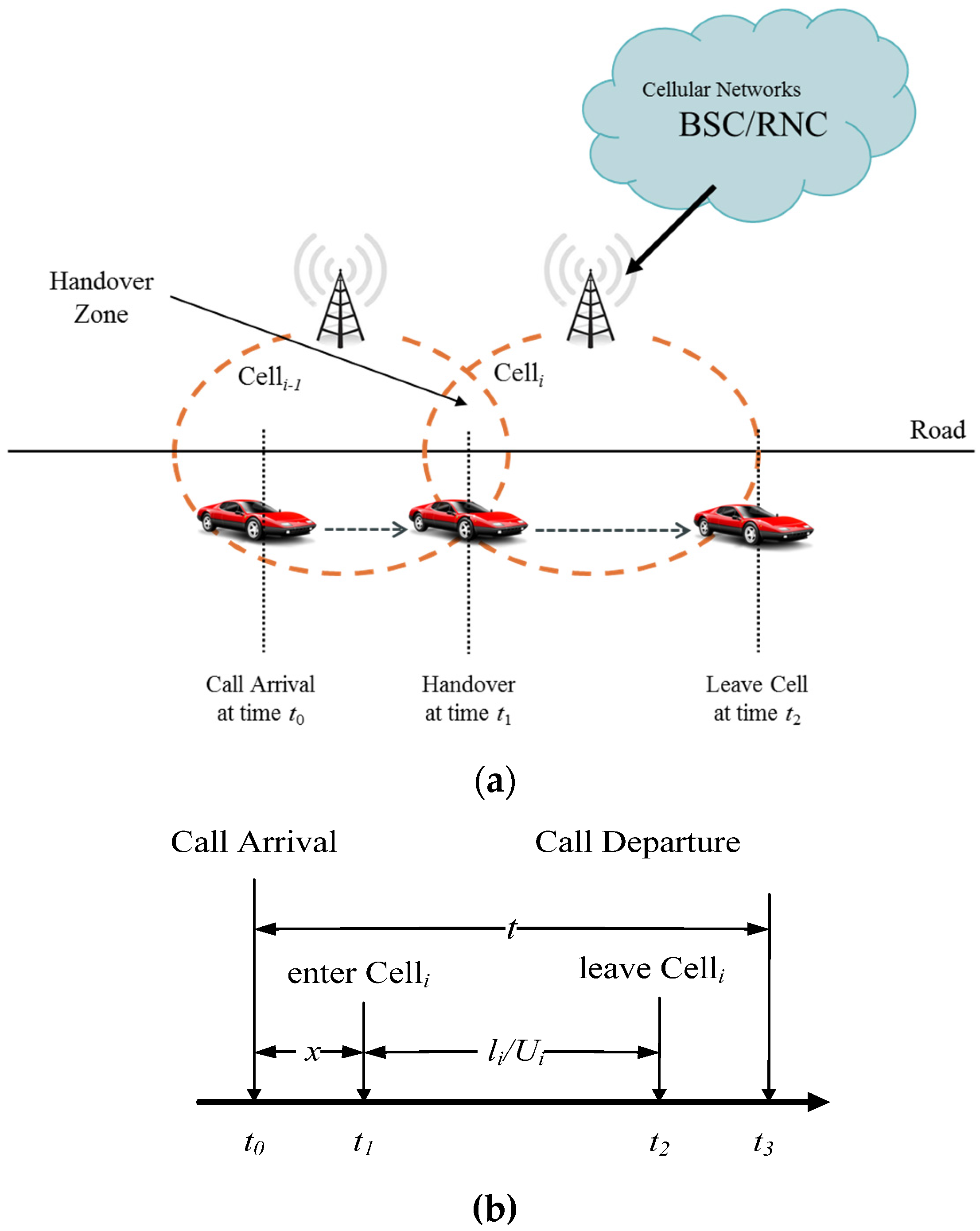
Figure 1a illustrates the space diagram for vehicle movement and the handover on a road. Figure 1b depicts the timing diagram for the handover on the road segment covered by Cell_i. The MS in a car performs the call set-up at time t₀ (in Figure 1a,b); then, the MS goes into the handover area of the coverage of Cell_i−1 and Cell_i at time t₁ (in Figure 1a,b), and the base station controller (BSC) or radio network controller (RNC) will allocate an available channel for the communicating MS. At this moment, if Cell_i has a free channel, the connection between the MS and Cell_i will be established successfully. The process is called a handover from Cell_i−1 to Cell_i.

Figure 1. (a) The scenario diagram for vehicle movement and the handover on the road; (b) the timing diagram for the handover on the road segment covered by Celli. BSC, base station controller; RNC, radio network controller.

Figure 1. (a) The scenario diagram for vehicle movement and the handover on the road; (b) the timing diagram for the handover on the road segment covered by Celli. BSC, base station controller; RNC, radio network controller.

This study assumes that the call holding time (t) is exponentially distributed with the mean $1/\mathsf{\mu }$ to generate handovers [25]. The average speed of cars is U_i, and the traffic flow is Q_i. Furthermore, the length of road segment covered by Celli is l_i. Let the variable x be the time difference between t₀ and t₁, and l_i/U_i denotes the time difference between t₁ and t₂. The handover procedure will be performed when the call holding time (t) is larger than x. Thereby, the amount of handover (h_i) on the road segment covered by Cell_i can be expressed as Equation (2), and this study can estimate traffic flow ($q_{i,h}$) by using Equation (3), which is the traffic flow multiplied by the number of HO events.

$$\begin{array}{ll}{h}_i& =Q_i\times {\displaystyle {\int }_{x=0}^{\infty }\mathrm{Pr}\left(t>x\right)dx}\\ & =Q_i\times {\displaystyle {\int }_{x=0}^{\infty }{\displaystyle {\int }_{t=x}^{\infty }\mathsf{\mu }{e}^{-\mathsf{\mu }t}dt}dx}\\ & =Q_i\times {\displaystyle {\int }_{x=0}^{\infty }\left({-e^{-\mathsf{\mu }t}|}_{t=x}^{\infty }\right)dx}=Q_i\times {\displaystyle {\int }_{x=0}^{\infty }{e}^{-\mathsf{\mu }x}dx}\\ & =Q_i\times \left({\frac{-e^{-\mathsf{\mu }x}}{\mathsf{\mu }}|}_{x=0}^{\infty }\right)=\frac{Q_i}{\mathsf{\mu }}\end{array}$$

(2)

$$q_{i,h}=h_i\times \mu$$

(3)

Traffic Flow Estimation by Using NLU Events

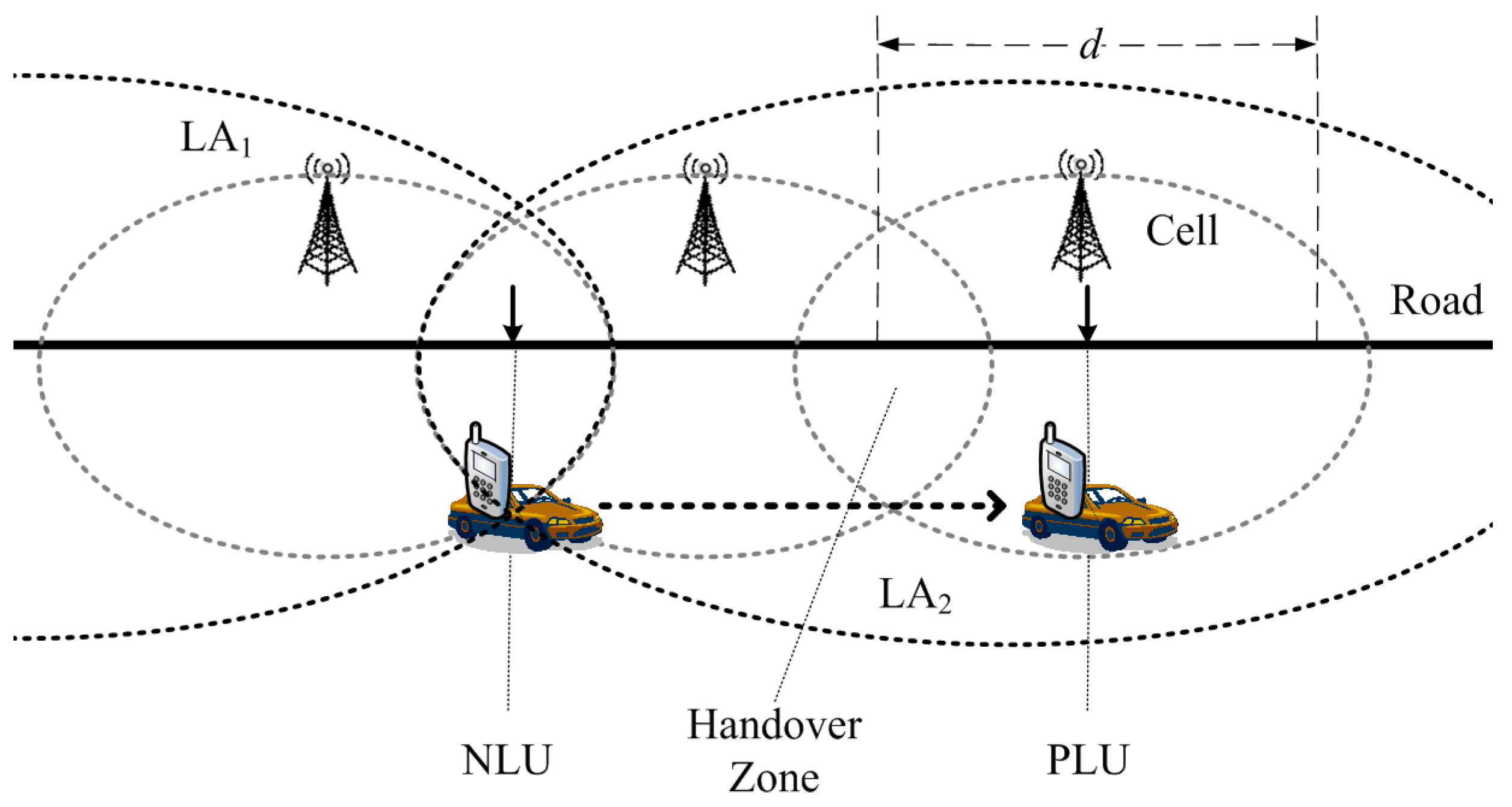
In cellular networks, the NLU event is generated when an MS moves from a location area (LA) to another LA. Therefore, traffic flow can be estimated by using the number of NLU events. This study assumes that the actual traffic flow on the road segment covered by Cell_i is $Q_i$ and one MS is in each car (shown in Figure 2) [24]. Therefore, the estimated traffic flow $q_{i,n}$ (i.e., the number of NLU events) on the road segment covered by Cell_i can be calculated as Equation (4), which is the traffic flow multiplied by the number of NLU events.

$$q_{i,n}=Q_i$$

(4)

Figure 2. The scenario diagram of location update events. LA, location area.

Figure 2. The scenario diagram of location update events. LA, location area.

3.1.2. Traffic Density Estimation

For traffic density estimation, this study considers the amount of CAs (a_i) and the amount of periodic location updates (PLUs) (p_i) to estimate traffic density (K_i) on the road segment covered by Cell_i.

Traffic Density Estimation by Using CA events

In cellular networks, a cell is supplied with radio service by vicinal BTSs or Node Bs. The BSC in GSM and RNC in UMTS are responsible for the network control. When a call arrives within the coverage area of a cell, the BSC or the RNC provides a free channel to the MS, and the MS will be connected with the corresponding base station if there is a free channel.

Figure 3a depicts the scenario diagram for vehicle movement and call arrivals on the road. Figure 4b shows the timing diagram for call arrivals on the road segment covered by a specific Cell_i. The MS in a car moving along the road performs the first call at time t₀ (in Figure 3a,b) and enters the coverage area of Cell_i at time t₁ (in Figure 3a,b). The MS performs another call at time t₂ (in Figure 3a,b) before leaving Cell_i (time t₃ in Figure 3a,b), and the call performed by the MS is called a call arrival in Cell_i.

Figure 3. (a) The scenario diagram for vehicle movement and call arrivals on the road; (b) the timing diagram for call arrivals on the road segment covered by Celli.

Figure 3. (a) The scenario diagram for vehicle movement and call arrivals on the road; (b) the timing diagram for call arrivals on the road segment covered by Celli.

This study assumes that the call inter-arrival time ($\mathsf{\tau }$) is exponentially distributed with the mean $1/\mathsf{\lambda }$ to generate call arrivals [25]. The length of road segment covered by Celli is l_i, and the average speed of cars is U_i. Therefore, l_i/U_i denotes the time difference between t₁ and t₃. This study analyzes the amount of call arrivals (a_i) that occur between t₁ and t₃ on the road segment covered by Cell_i. The amount of call arrivals can be expressed as Equation (5), and Equation (6) indicates that this study can derive estimated traffic density ($k_{i,a}$) from the amount of call arrivals.

$$\begin{array}{ll}{a}_i& =Q_i\times \mathrm{Pr}\left[t_1<t_2<t_3\right]\\ & =Q_i\times {\displaystyle {\int }_{x=0}^{\infty }\mathrm{Pr}\left[x<\mathsf{\tau }<x+\frac{l_i}{U_i}\right]dx}\\ & =Q_i\times {\displaystyle {\int }_{x=0}^{\infty }{\displaystyle {\int }_{\mathsf{\tau }=x}^{x+\frac{l_i}{U_i}}\mathsf{\lambda }{e}^{-\mathsf{\lambda }\mathsf{\tau }}d\mathsf{\tau }}dx}\\ & =Q_i\times \frac{1-e^{-\frac{\mathsf{\lambda }{l}_i}{U_i}}}{\mathsf{\lambda }}\\ \Rightarrow & Q_i\left[1-{\left(1-\frac{\mathsf{\lambda }{a}_i}{Q_i}\right)}^{\frac{1}{\mathsf{\lambda }{l}_i}}\right]\approx \frac{Q_i}{U_i}=K_i, \text{where} \underset{U_i\to \infty }{\lim }1-e^{-\frac{1}{U_i}}=\frac{1}{U_i}\end{array}$$

(5)

$$k_{i,a}=q_i\left[1-{\left(1-\frac{\mathsf{\lambda }{a}_i}{q_i}\right)}^{\frac{1}{\mathsf{\lambda }{l}_i}}\right]\approx \frac{Q_i}{U_i}=K_i ,\text{where} \underset{U_i\to \infty }{\lim }1-e^{-\frac{1}{U_i}}=\frac{1}{U_i}$$

(6)

Traffic Density Estimation by Using PLU Events

For mobility management, the MS periodically performs the PLU event for the core network in cellular networks. Some MSs may perform the PLU event across the cell in Figure 2. Therefore, the probability models shown in Equations (7) and (8) are proposed to provide estimated vehicle density $k_{i,p}$ (i.e., the number of MS) on the road segment covered by Cell_i according to the number of PLU events. This model had been proven in [24,38], and this study summarizes the assumptions in this model as follows.

•

The actual vehicle density $K_i$ and traffic speed $U_i$ can be obtained from VD on the road. Furthermore, the length of a road segment covered by the cell is $l$.

•

The call arrival rate to a cell is $\mathsf{\lambda }$, and the call arrival process is assumed to be a Poisson process.

•

The cycle time of PLU is $b$, and the number of PLU events is $p_i$.

$$\begin{array}{ll}{p}_i& =Q_i\times \mathrm{Pr}(\text{PLU})\\ & =Q_i\times (3-e^{-\mathsf{\lambda }b})\times \left(e^{-\mathsf{\lambda }b}\frac{l}{2U_{i}b}\right)\\ & =K_i\times (3-e^{-\mathsf{\lambda }b})\times \left(e^{-\mathsf{\lambda }b}\frac{l}{2U_{i}b}\right)\end{array}$$

(7)

$$k_{i,p}=\frac{p_i}{\left(3-e^{-\mathsf{\lambda }b}\right)\times \left(e^{-\mathsf{\lambda }b}\frac{l}{2U_{i}b}\right)}$$

(8)

3.1.3. Vehicle Speed Estimation

In this paper, the vehicle speed is obtained by the estimated traffic flow by using HO events (q_i,h), the estimated traffic flow by using NLU events (q_i,n), the estimated traffic density by using CA events (k_i,a) and the estimated traffic density by using PLU events (k_i,p). Based on Section 3.1.1 and Section 3.1.2, the estimated vehicle speeds $u_{i,ha}$, $u_{i,na}$, $u_{i,hp}$ and $u_{i,np}$ can be expressed as Equations (9)–(12). For instance, the estimated vehicle speed $u_{i,ha}$ can be obtained by using q_i,h and k_i,a; the estimated vehicle speed $u_{i,na}$ can be obtained by using q_i,n and k_i,a; the estimated vehicle speed $u_{i,hp}$ can be obtained by using q_i,h and k_i,p; the estimated vehicle speed $u_{i,np}$ can be obtained by using q_i,n and k_i,p.

$$u_{i,ha}=\frac{q_{i,h}}{k_{i,a}}={\left[1-{\left(1-\frac{\mathsf{\lambda }{a}_i}{\mathsf{\mu }{h}_i}\right)}^{\frac{1}{\mathsf{\lambda }{l}_i}}\right]}^{-1}$$

(9)

$$u_{i,na}=\frac{q_{i,n}}{k_{i,a}}={\left[1-{\left(1-\frac{\mathsf{\lambda }{a}_i}{q_{i,n}}\right)}^{\frac{1}{\mathsf{\lambda }{l}_i}}\right]}^{-1}$$

(10)

$$u_{i,hp}=\frac{q_{i,h}}{k_{i,p}}=\frac{\mathsf{\mu }{h}_i(3-e^{-\mathsf{\lambda }b})\left(e^{-\mathsf{\lambda }b}\frac{l}{2U_{i}b}\right)}{p_i}$$

(11)

$$u_{i,np}=\frac{q_{i,n}}{k_{i,p}}=\frac{q_{i,n}(3-e^{-\mathsf{\lambda }b})\left(e^{-\mathsf{\lambda }b}\frac{l}{2U_{i}b}\right)}{p_i}$$

(12)

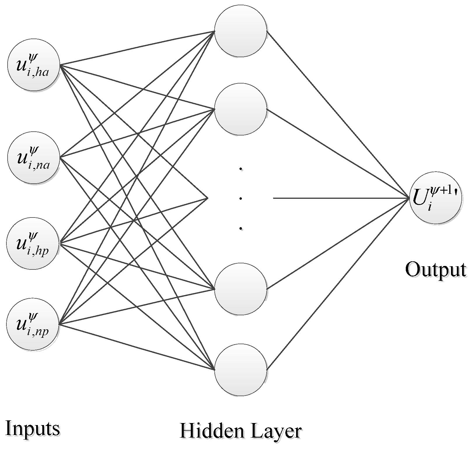
3.2. Vehicle Speed Forecasting Method

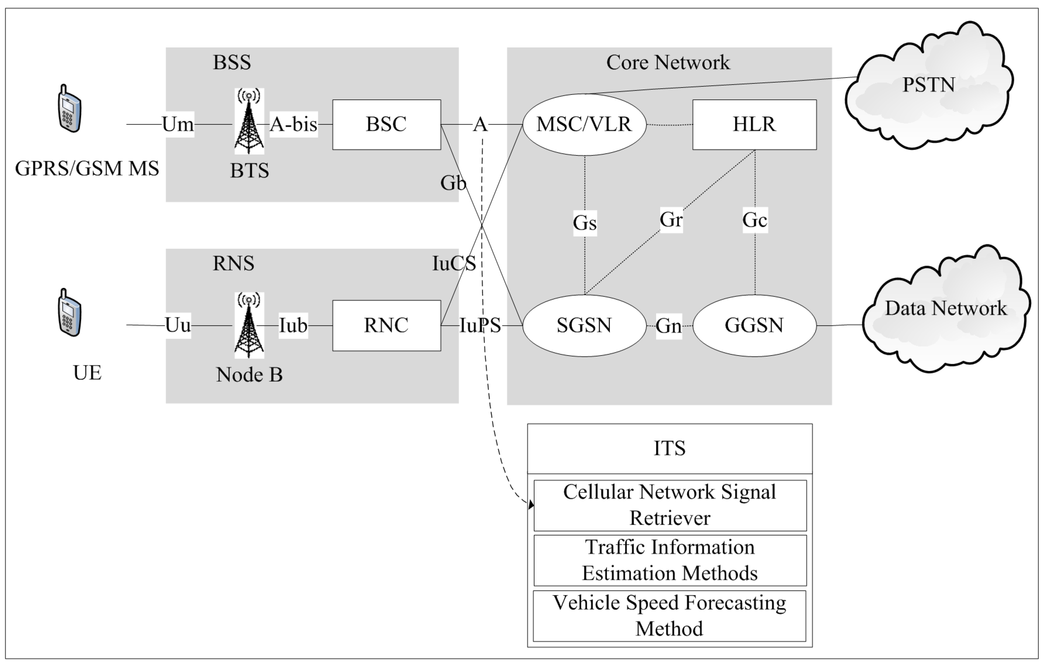
For vehicle speed prediction, a BPNN algorithm is considered to predict the future vehicle speed in accordance with the current traffic information (i.e., the estimated vehicle speeds from CFVD in Section 3.1). An intelligent transportation system, which includes a cellular network signal retriever (CNSR), traffic information estimation methods and a vehicle speed forecasting method, has been designed and implemented for traffic information estimation and prediction (shown in Figure 4). The ITS can retrieve cellular network signals (e.g., NLU, PLU, HO and CA) via the A interface and the IuCS interface and analyze these signals to estimate traffic information (e.g., traffic flow, traffic density and vehicle speed). Then, the estimated vehicle speed can be adopted as input characteristics into the proposed vehicle speed forecasting method to predict short-term vehicle speed for road user decision.

In this subsection, the average vehicle speed of road segment i at cycle $\mathsf{\psi }$ is expressed as $U_i^{\mathsf{\psi }}$, and the estimated vehicle speed at cycle $\mathsf{\psi }$ in accordance with Equations (9)–(12) can be expressed as $u_{i,ha}^{\mathsf{\psi }}$, $u_{i,na}^{\mathsf{\psi }}$, $u_{i,hp}^{\mathsf{\psi }}$ and $u_{i,np}^{\mathsf{\psi }}$, respectively. This study collects the values of the current traffic information (i.e., $u_{i,ha}^{\mathsf{\psi }}$, $u_{i,na}^{\mathsf{\psi }}$, $u_{i,hp}^{\mathsf{\psi }}$ and $u_{i,np}^{\mathsf{\psi }}$) as the input characteristics of the neurons in the BPNN to predict the future vehicle speed (i.e., $U_i^{\mathsf{\psi }+1}$) (see Figure 5). Therefore, the number of neurons in the input layer is four. There is one hidden layer, and the output value of the predicted vehicle speed $U_i^{\mathsf{\psi }+1}\text{'}$ can be obtained by BPNN.

Figure 4. Intelligent transportation system based on the proposed methods.

Figure 4. Intelligent transportation system based on the proposed methods.

Figure 5. Vehicle speed estimation based on the back-propagation neural network algorithm.

Figure 5. Vehicle speed estimation based on the back-propagation neural network algorithm.

In the training stage, the historical datasets of cellular network signals from CNSR and traffic information from VDs are collected and calculated the amount of NLU, PLU, HO and CA events. Then vehicle speed can be estimated in accordance with the estimated traffic flows by using NLU and HO events and the estimated traffic densities by using PLU and CA events to obtain the values of $u_{i,ha}^{\mathsf{\psi }}$, $u_{i,na}^{\mathsf{\psi }}$, $u_{i,hp}^{\mathsf{\psi }}$ and $u_{i,np}^{\mathsf{\psi }}$ at cycle $\mathsf{\psi }$. Moreover, the average vehicle speed $U_i^{\mathsf{\psi }+1}$ of road segment i at next cycle ($\mathsf{\psi }$ + 1) can be collected by VD. The proposed vehicle speed forecasting method based on BPNN adopts $u_{i,ha}^{\mathsf{\psi }}$, $u_{i,na}^{\mathsf{\psi }}$, $u_{i,hp}^{\mathsf{\psi }}$ and $u_{i,np}^{\mathsf{\psi }}$ as input characteristics and $U_i^{\mathsf{\psi }+1}$ as the output characteristic to train a neural network.

In the runtime stage, the real-time estimated vehicle speeds can be obtained by the proposed traffic information estimation methods based on using CFVD. Then, the estimated vehicle speeds ($u_{i,ha}$, $u_{i,na}$, $u_{i,hp}$ and $u_{i,np}$) of road segment i can be adopted into the trained neural network in the training stage to forecast the short-term vehicle speed at the next cycle.

4. Experimental Results and Analyses

This section adopts the practical traffic information (i.e., traffic flow and vehicle speed) from Taiwan Area National Freeway Bureau as the input characteristics of the traffic simulation program and refers to the MS communication behaviors from Chunghwa Telecom to simulate the traffic information and communication records. The details of the experimental environments are presented in Section 4.1. The traffic information estimation and forecasting methods are illustrated in Section 4.2 and Section 4.3.

4.1. Experimental Environments

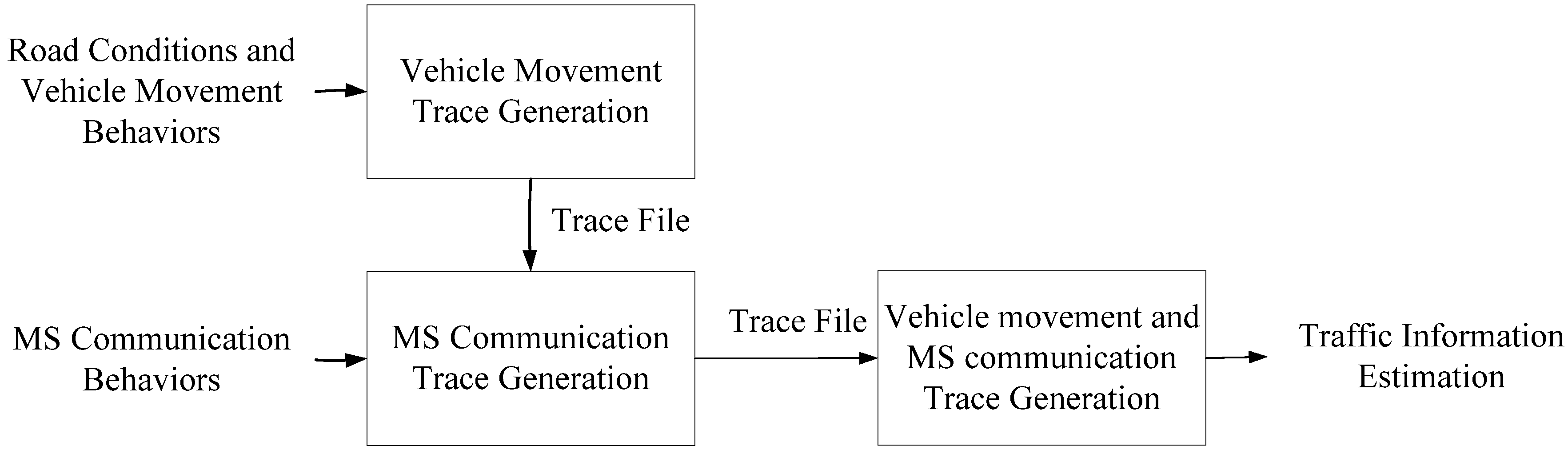
In this study, trace-driven experiments, which consider vehicle movement traces and MS communication traces, are designed to evaluate the traffic information estimation and forecasting methods based on CFVD (shown in Figure 6). The inputs of the trace generator include the road conditions (e.g., the length of the road, the number of lanes, the locations of handover points and traffic flows), the vehicle movement behaviors (e.g., vehicles speeds, car following model and lane-changing model) and MS communication behaviors (e.g., call inter-arrival time and call holding time). The output is a trace file, which records the vehicle’s ID, vehicle speed, its CAs, its HOs, its NLUs and its PLUs. For the generation of vehicle movement traces, the practical traffic information, which included traffic flows and vehicle speeds from VDs on National Highway No. 3 in Taiwan during October in 2010, was collected and expressed as the characteristics of road conditions (i.e., traffic flows) and vehicle movement behaviors (i.e., vehicle speeds) for traffic simulation. Furthermore, call holding time is exponentially distributed with the mean $1/\mathsf{\mu }$, and the call inter-arrival time is exponentially distributed with the mean $1/\mathsf{\lambda }$ in accordance with the mobile communication records from Chunghwa Telecom for the generation of MS communication traces [13]. Then, vehicle movement and MS communication traces can be generated by a traffic simulation program, VISSIM. 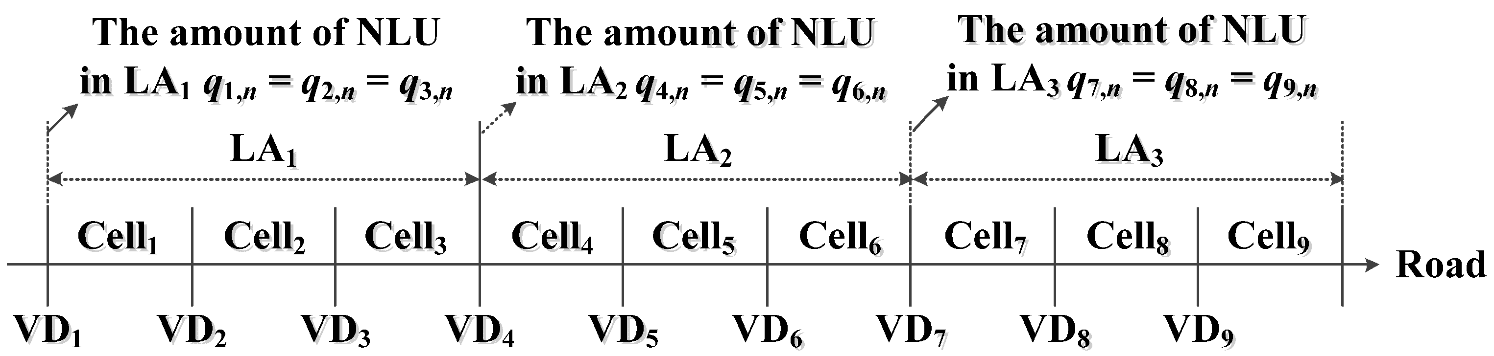Figure 7 shows nine handover points and nine cells distributed in three location areas on the road from 0–9 km, and the coverage of a cell is 1 km. Moreover, this study assumes that there are nine VDs, which are built in the same locations with handover points for evaluating the traffic information of each road segment covered by a cell.

Figure 6. Trace-driven simulation for the traffic information estimations.

Figure 6. Trace-driven simulation for the traffic information estimations.

Figure 7. The distribution of cells, location areas and vehicle detectors (VDs) in the simulation experiments.

Figure 7. The distribution of cells, location areas and vehicle detectors (VDs) in the simulation experiments.

4.2. The Evaluation of Traffic Information Estimation Methods

The proposed analytic models were evaluated for the evaluation of traffic flow estimation based on the amount of HOs and NLUs and the evaluation of traffic density estimation based on the amount of CAs and PLUs in Section 4.2.1 and Section 4.2.2. Finally, the vehicle speed estimation methods based on the estimated traffic flow and the estimated traffic density were evaluated in Section 4.2.3.

4.2.1. The Evaluation of Traffic Flow Estimation

For the evaluation of traffic flow estimation, the simulated amounts of HOs and NLUs from Cell_i are collected as CFVD to generate $q_{i,h}$ and $q_{i,n}$. NLU is only performed with MS entering new LA, so the estimated traffic flows are consistence in the same LA in the proposed approach. For instance, the amount of HOs in Cell₁ ($h_1$) was 126 at 8 a.m. and 9 a.m., so the traffic flow of the first road segment ($q_{1,h}$) could be estimated as 7560 car/h by utilizing Equation (3) and MS communication behaviors (e.g., the expected value ($1/\mathsf{\mu }$) of call holding time is 1 min/call). Furthermore, because 6672 NLUs in Cell₁ were performed at 8 a.m. and 9 a.m., the traffic flow of the first road segment ($q_{1,n}$) could be estimated as 6672 car/h according to Equation (4). This study calculated the accuracies of traffic flow estimation as $1-\frac{\left|Q_i-q_{i,h}\right|}{Q_i}$ and $1-\frac{\left|Q_i-q_{i,n}\right|}{Q_i}$. Table 2 shows that the average accuracies of traffic flow estimation of the first road segment between 8 a.m. and 22 p.m. are 89% for the amount of HOs and 100% for the amount of NLUs. As shown in Table 3, the comparison of the traffic flow estimation comparisons between $q_{1,h}$ and $q_{i,n}$ indicates that the amount of NLUs is more suitable for traffic flow estimation than the amount of HOs.

Table 2. The accuracies of traffic flow estimation of the road segment covered by Cell₁.

Time	Q1	The Amount of HOs	The Amount of NLUs	${\mathit{q}}_{\mathbf{1}\mathbf{,}\mathit{h}}$	${\mathit{q}}_{\mathbf{1}\mathbf{,}\mathit{n}}$	$\mathbf{1}\mathbf{-}\frac{\mathbf{\left|}{\mathit{Q}}_{\mathbf{1}}\mathbf{-}{\mathit{q}}_{\mathbf{1}\mathbf{,}\mathit{h}}\mathbf{\right|}}{{\mathit{Q}}_{\mathbf{1}}}$	$\mathbf{1}\mathbf{-}\frac{\mathbf{\left|}{\mathit{Q}}_{\mathbf{1}}\mathbf{-}{\mathit{q}}_{\mathbf{1}\mathbf{,}\mathit{n}}\mathbf{\right|}}{{\mathit{Q}}_{\mathbf{1}}}$
8	6672	126	6672	7560	6672	87%	100%
9	6200	112	6200	6720	6200	92%	100%
10	5435	92	5435	5520	5435	98%	100%
11	5663	80	5663	4800	5663	85%	100%
12	5532	90	5532	5400	5532	98%	100%
13	5265	90	5265	5400	5265	97%	100%
14	5546	90	5546	5400	5546	97%	100%
15	6368	88	6368	5280	6368	83%	100%
16	5762	78	5762	4680	5762	81%	100%
17	6101	124	6101	7440	6101	78%	100%
18	6122	104	6122	6240	6122	98%	100%
19	5378	74	5378	4440	5378	83%	100%
20	4667	72	4667	4320	4667	93%	100%
21	4625	64	4625	3840	4625	83%	100%
22	4312	60	4312	3600	4312	83%	100%
Mean						89%	100%

Table 2. The accuracies of traffic flow estimation of the road segment covered by Cell₁.

Time	Q1	The Amount of HOs	The Amount of NLUs	${\mathit{q}}_{\mathbf{1}\mathbf{,}\mathit{h}}$	${\mathit{q}}_{\mathbf{1}\mathbf{,}\mathit{n}}$	$\mathbf{1}\mathbf{-}\frac{\mathbf{\left|}{\mathit{Q}}_{\mathbf{1}}\mathbf{-}{\mathit{q}}_{\mathbf{1}\mathbf{,}\mathit{h}}\mathbf{\right|}}{{\mathit{Q}}_{\mathbf{1}}}$	$\mathbf{1}\mathbf{-}\frac{\mathbf{\left|}{\mathit{Q}}_{\mathbf{1}}\mathbf{-}{\mathit{q}}_{\mathbf{1}\mathbf{,}\mathit{n}}\mathbf{\right|}}{{\mathit{Q}}_{\mathbf{1}}}$
8	6672	126	6672	7560	6672	87%	100%
9	6200	112	6200	6720	6200	92%	100%
10	5435	92	5435	5520	5435	98%	100%
11	5663	80	5663	4800	5663	85%	100%
12	5532	90	5532	5400	5532	98%	100%
13	5265	90	5265	5400	5265	97%	100%
14	5546	90	5546	5400	5546	97%	100%
15	6368	88	6368	5280	6368	83%	100%
16	5762	78	5762	4680	5762	81%	100%
17	6101	124	6101	7440	6101	78%	100%
18	6122	104	6122	6240	6122	98%	100%
19	5378	74	5378	4440	5378	83%	100%
20	4667	72	4667	4320	4667	93%	100%
21	4625	64	4625	3840	4625	83%	100%
22	4312	60	4312	3600	4312	83%	100%
Mean						89%	100%

Table 3. The accuracies of traffic flow estimation of each road segment.

Cell	$\mathbf{1}\mathbf{-}\frac{\mathbf{\left|}{\mathit{Q}}_{\mathit{i}}\mathbf{-}{\mathit{q}}_{\mathit{i}\mathbf{,}\mathit{h}}\mathbf{\right|}}{{\mathit{Q}}_{\mathit{i}}}$	$\mathbf{1}\mathbf{-}\frac{\mathbf{\left|}{\mathit{Q}}_{\mathit{i}}\mathbf{-}{\mathit{q}}_{\mathit{i}\mathbf{,}\mathit{n}}\mathbf{\right|}}{{\mathit{Q}}_{\mathit{i}}}$
Cell1	89%	100%
Cell2	76%	100%
Cell3	77%	100%
Cell4	78%	100%
Cell5	70%	100%
Cell6	67%	99%
Cell7	68%	100%
Cell8	70%	100%
Cell9	72%	100%
Mean	74%	100%

Table 3. The accuracies of traffic flow estimation of each road segment.

Cell	$\mathbf{1}\mathbf{-}\frac{\mathbf{\left|}{\mathit{Q}}_{\mathit{i}}\mathbf{-}{\mathit{q}}_{\mathit{i}\mathbf{,}\mathit{h}}\mathbf{\right|}}{{\mathit{Q}}_{\mathit{i}}}$	$\mathbf{1}\mathbf{-}\frac{\mathbf{\left|}{\mathit{Q}}_{\mathit{i}}\mathbf{-}{\mathit{q}}_{\mathit{i}\mathbf{,}\mathit{n}}\mathbf{\right|}}{{\mathit{Q}}_{\mathit{i}}}$
Cell1	89%	100%
Cell2	76%	100%
Cell3	77%	100%
Cell4	78%	100%
Cell5	70%	100%
Cell6	67%	99%
Cell7	68%	100%
Cell8	70%	100%
Cell9	72%	100%
Mean	74%	100%

4.2.2. The Evaluation of Traffic Density Estimation

For the evaluation of traffic density estimation, the simulated amounts of CAs and PLUs from Cell_i are collected as CFVD to generate $k_{i,a}$ and $k_{i,p}$. For instance, the amount of CAs in Cell₁ ($a_1$) was 97 at 8 a.m., so the traffic density of the first road segment ($k_{1,a}$) could be estimated as 97 car/km by Equation (6) and MS communication behaviors (e.g., the expected value ($1/\mathsf{\lambda }$) of the call inter-arrival time is 1 h/call). Furthermore, because 126 PLUs were performed in Cell₁ at 8 a.m., the traffic density of the first road segment ($k_{1,p}$) could be estimated as 128 car/h in accordance with Equation (8) and MS communication behaviors (e.g., call inter-arrival time). This study calculated the accuracies of traffic density estimation as $1-\frac{\left|K_i-k_{i,a}\right|}{K_i}$ and $1-\frac{\left|K_i-k_{i,p}\right|}{K_i}$. Table 4 shows that the average accuracies of traffic density estimation of the first road segment between 8 a.m. and 22 p.m. are 91% for the amount of CAs and 81% for the amount of PLUs. As shown in Table 5, the results of the traffic density estimation between $k_{i,a}$ and $k_{i,p}$ indicate that the amount of CAs is more suitable for traffic density estimation than the amount of PLUs.

Table 4. The accuracies of traffic density estimation of the road segment covered by Cell₁.

Time	K1	The Amount of CAs	The Amount of PLUs	${\mathit{k}}_{\mathbf{1}\mathbf{,}\mathit{a}}$	${\mathit{k}}_{\mathbf{1}\mathbf{,}\mathit{p}}$	$\mathbf{1}\mathbf{-}\frac{\mathbf{\left|}{\mathit{K}}_{\mathbf{1}}\mathbf{-}{\mathit{k}}_{\mathbf{1}\mathbf{,}\mathit{a}}\mathbf{\right|}}{{\mathit{K}}_{\mathbf{1}}}$	$\mathbf{1}\mathbf{-}\frac{\mathbf{\left|}{\mathit{K}}_{\mathbf{1}}\mathbf{-}{\mathit{k}}_{\mathbf{1}\mathbf{,}\mathit{p}}\mathbf{\right|}}{{\mathit{K}}_{\mathbf{1}}}$
8	97	97	126	97	128	99%	67%
9	88	86	112	86	103	97%	83%
10	77	71	92	71	81	93%	95%
11	69	62	80	62	74	90%	92%
12	67	69	90	69	58	96%	87%
13	63	69	90	69	70	91%	89%
14	67	69	90	69	74	97%	89%
15	78	68	88	68	99	87%	72%
16	70	60	78	60	85	86%	78%
17	87	96	124	96	105	89%	78%
18	87	80	104	80	105	92%	79%
19	76	57	74	57	97	75%	72%
20	56	55	72	55	60	99%	92%
21	55	49	64	49	70	89%	73%
22	51	46	60	46	64	90%	75%
Mean						91%	81%

Table 4. The accuracies of traffic density estimation of the road segment covered by Cell₁.

Time	K1	The Amount of CAs	The Amount of PLUs	${\mathit{k}}_{\mathbf{1}\mathbf{,}\mathit{a}}$	${\mathit{k}}_{\mathbf{1}\mathbf{,}\mathit{p}}$	$\mathbf{1}\mathbf{-}\frac{\mathbf{\left|}{\mathit{K}}_{\mathbf{1}}\mathbf{-}{\mathit{k}}_{\mathbf{1}\mathbf{,}\mathit{a}}\mathbf{\right|}}{{\mathit{K}}_{\mathbf{1}}}$	$\mathbf{1}\mathbf{-}\frac{\mathbf{\left|}{\mathit{K}}_{\mathbf{1}}\mathbf{-}{\mathit{k}}_{\mathbf{1}\mathbf{,}\mathit{p}}\mathbf{\right|}}{{\mathit{K}}_{\mathbf{1}}}$
8	97	97	126	97	128	99%	67%
9	88	86	112	86	103	97%	83%
10	77	71	92	71	81	93%	95%
11	69	62	80	62	74	90%	92%
12	67	69	90	69	58	96%	87%
13	63	69	90	69	70	91%	89%
14	67	69	90	69	74	97%	89%
15	78	68	88	68	99	87%	72%
16	70	60	78	60	85	86%	78%
17	87	96	124	96	105	89%	78%
18	87	80	104	80	105	92%	79%
19	76	57	74	57	97	75%	72%
20	56	55	72	55	60	99%	92%
21	55	49	64	49	70	89%	73%
22	51	46	60	46	64	90%	75%
Mean						91%	81%

Table 5. The accuracies of traffic density estimation of each road segment.

Cell	$\mathbf{1}\mathbf{-}\frac{\mathbf{\left|}{\mathit{K}}_{\mathit{i}}\mathbf{-}{\mathit{k}}_{\mathit{i}\mathbf{,}\mathit{a}}\mathbf{\right|}}{{\mathit{K}}_{\mathit{i}}}$	$\mathbf{1}\mathbf{-}\frac{\mathbf{\left|}{\mathit{K}}_{\mathit{i}}\mathbf{-}{\mathit{k}}_{\mathit{i}\mathbf{,}\mathit{p}}\mathbf{\right|}}{{\mathit{K}}_{\mathit{i}}}$
Cell1	91%	81%
Cell2	88%	75%
Cell3	90%	70%
Cell4	86%	86%
Cell5	84%	75%
Cell6	88%	73%
Cell7	86%	76%
Cell8	87%	84%
Cell9	84%	73%
Mean	87%	77%

Table 5. The accuracies of traffic density estimation of each road segment.

Cell	$\mathbf{1}\mathbf{-}\frac{\mathbf{\left|}{\mathit{K}}_{\mathit{i}}\mathbf{-}{\mathit{k}}_{\mathit{i}\mathbf{,}\mathit{a}}\mathbf{\right|}}{{\mathit{K}}_{\mathit{i}}}$	$\mathbf{1}\mathbf{-}\frac{\mathbf{\left|}{\mathit{K}}_{\mathit{i}}\mathbf{-}{\mathit{k}}_{\mathit{i}\mathbf{,}\mathit{p}}\mathbf{\right|}}{{\mathit{K}}_{\mathit{i}}}$
Cell1	91%	81%
Cell2	88%	75%
Cell3	90%	70%
Cell4	86%	86%
Cell5	84%	75%
Cell6	88%	73%
Cell7	86%	76%
Cell8	87%	84%
Cell9	84%	73%
Mean	87%	77%

4.2.3. The Evaluation of Vehicle Speed Estimation

For the evaluation of vehicle speed estimation, the estimated vehicle speeds $u_{i,ha}$, $u_{i,na}$, $u_{i,hp}$ and $u_{i,np}$ can be generated via the estimated traffic flow from HO events (q_i,h) Equation (3), the estimated traffic flow by using NLU events (q_i,n) Equation (4), the estimated traffic density by using CA events (k_i,a) and the estimated traffic density by using PLU events (k_i,p) by Equations (9)–(12). For instance, the average vehicle speed of the first road segment $u_{1,ha}$ can be estimated as 78 km/h (i.e., $u_{1,ha}=q_{1,h}/k_{1,a}$) at 8 a.m. in accordance with the estimated traffic flow by using HO events (i.e., q_1,h = 7560 car/h) and the estimated traffic density by using CA events (i.e., k_1,a = 97 car/km). This study calculated the accuracies of traffic density estimation as $1-\frac{\left|U_i-u_{i,ha}\right|}{U_i}$, $1-\frac{\left|U_i-u_{i,na}\right|}{U_i}$, $1-\frac{\left|U_i-u_{i,hp}\right|}{U_i}$ and $1-\frac{\left|U_i-u_{i,np}\right|}{U_i}$. In accordance with the results in Section 4.2.1 and Section 4.2.2, Table 6 shows that the average accuracies of vehicle speed estimation of the first road segment between 8 a.m. and 22 p.m. are 92%, 90%, 81% and 85% for the estimated vehicle speeds $u_{i,ha}$, $u_{i,na}$, $u_{i,hp}$ and $u_{i,np}$, respectively. As shown in Table 7, the results of the vehicle speed estimation show that the estimated traffic flow based on the amount of NLUs and estimated traffic density based on the amount of CAs can obtain the highest accuracy of vehicle speed estimation.

Table 6. The accuracies of vehicle speed estimation of the road segment covered by Cell₁.

Time	U1	${\mathit{u}}_{\mathbf{1}\mathbf{,}\mathit{h}\mathit{a}}$	${\mathit{u}}_{\mathbf{1}\mathbf{,}\mathit{n}\mathit{a}}$	${\mathit{u}}_{\mathbf{1}\mathbf{,}\mathit{h}\mathit{p}}$	${\mathit{u}}_{\mathbf{1}\mathbf{,}\mathit{n}\mathit{p}}$	$\mathbf{1}\mathbf{-}\frac{\mathbf{\left|}{\mathit{U}}_{\mathbf{1}}\mathbf{-}{\mathit{u}}_{\mathbf{1}\mathbf{,}\mathit{h}\mathit{a}}\mathbf{\right|}}{{\mathit{U}}_{\mathbf{1}}}$	$\mathbf{1}\mathbf{-}\frac{\mathbf{\left|}{\mathit{U}}_{\mathbf{1}}\mathbf{-}{\mathit{u}}_{\mathbf{1}\mathbf{,}\mathit{n}\mathit{a}}\mathbf{\right|}}{{\mathit{U}}_{\mathbf{1}}}$	$\mathbf{1}\mathbf{-}\frac{\mathbf{\left|}{\mathit{U}}_{\mathbf{1}}\mathbf{-}{\mathit{u}}_{\mathbf{1}\mathbf{,}\mathit{h}\mathit{p}}\mathbf{\right|}}{{\mathit{U}}_{\mathbf{1}}}$	$\mathbf{1}\mathbf{-}\frac{\mathbf{\left|}{\mathit{U}}_{\mathbf{1}}\mathbf{-}{\mathit{u}}_{\mathbf{1}\mathbf{,}\mathit{n}\mathit{p}}\mathbf{\right|}}{{\mathit{U}}_{\mathbf{1}}}$
8	69	78	69	59	52	87%	99%	85%	75%
9	70	78	72	65	60	89%	97%	93%	86%
10	71	78	77	69	67	90%	92%	97%	95%
11	83	77	91	65	76	94%	89%	78%	92%
12	83	78	80	93	96	94%	96%	88%	85%
13	83	78	76	77	75	94%	92%	92%	90%
14	83	78	80	73	75	94%	97%	88%	90%
15	82	78	94	53	64	95%	86%	65%	78%
16	83	78	96	55	68	94%	84%	67%	82%
17	70	78	64	71	58	90%	90%	100%	82%
18	70	78	77	59	58	89%	91%	84%	83%
19	71	78	94	46	55	90%	67%	65%	78%
20	84	79	85	72	78	94%	99%	86%	93%
21	84	78	94	55	66	93%	87%	65%	79%
22	84	78	94	56	67	93%	89%	67%	80%
Mean						92%	90%	81%	85%

Table 6. The accuracies of vehicle speed estimation of the road segment covered by Cell₁.

Time	U1	${\mathit{u}}_{\mathbf{1}\mathbf{,}\mathit{h}\mathit{a}}$	${\mathit{u}}_{\mathbf{1}\mathbf{,}\mathit{n}\mathit{a}}$	${\mathit{u}}_{\mathbf{1}\mathbf{,}\mathit{h}\mathit{p}}$	${\mathit{u}}_{\mathbf{1}\mathbf{,}\mathit{n}\mathit{p}}$	$\mathbf{1}\mathbf{-}\frac{\mathbf{\left|}{\mathit{U}}_{\mathbf{1}}\mathbf{-}{\mathit{u}}_{\mathbf{1}\mathbf{,}\mathit{h}\mathit{a}}\mathbf{\right|}}{{\mathit{U}}_{\mathbf{1}}}$	$\mathbf{1}\mathbf{-}\frac{\mathbf{\left|}{\mathit{U}}_{\mathbf{1}}\mathbf{-}{\mathit{u}}_{\mathbf{1}\mathbf{,}\mathit{n}\mathit{a}}\mathbf{\right|}}{{\mathit{U}}_{\mathbf{1}}}$	$\mathbf{1}\mathbf{-}\frac{\mathbf{\left|}{\mathit{U}}_{\mathbf{1}}\mathbf{-}{\mathit{u}}_{\mathbf{1}\mathbf{,}\mathit{h}\mathit{p}}\mathbf{\right|}}{{\mathit{U}}_{\mathbf{1}}}$	$\mathbf{1}\mathbf{-}\frac{\mathbf{\left|}{\mathit{U}}_{\mathbf{1}}\mathbf{-}{\mathit{u}}_{\mathbf{1}\mathbf{,}\mathit{n}\mathit{p}}\mathbf{\right|}}{{\mathit{U}}_{\mathbf{1}}}$
8	69	78	69	59	52	87%	99%	85%	75%
9	70	78	72	65	60	89%	97%	93%	86%
10	71	78	77	69	67	90%	92%	97%	95%
11	83	77	91	65	76	94%	89%	78%	92%
12	83	78	80	93	96	94%	96%	88%	85%
13	83	78	76	77	75	94%	92%	92%	90%
14	83	78	80	73	75	94%	97%	88%	90%
15	82	78	94	53	64	95%	86%	65%	78%
16	83	78	96	55	68	94%	84%	67%	82%
17	70	78	64	71	58	90%	90%	100%	82%
18	70	78	77	59	58	89%	91%	84%	83%
19	71	78	94	46	55	90%	67%	65%	78%
20	84	79	85	72	78	94%	99%	86%	93%
21	84	78	94	55	66	93%	87%	65%	79%
22	84	78	94	56	67	93%	89%	67%	80%
Mean						92%	90%	81%	85%

Table 7. The accuracies of vehicle speed estimation of each road segment.

Cell	$\mathbf{1}\mathbf{-}\frac{\mathbf{\left|}{\mathit{U}}_{\mathit{i}}\mathbf{-}{\mathit{u}}_{\mathit{i}\mathbf{,}\mathit{h}\mathit{a}}\mathbf{\right|}}{{\mathit{U}}_{\mathit{i}}}$	$\mathbf{1}\mathbf{-}\frac{\mathbf{\left|}{\mathit{U}}_{\mathit{i}}\mathbf{-}{\mathit{u}}_{\mathit{i}\mathbf{,}\mathit{n}\mathit{a}}\mathbf{\right|}}{{\mathit{U}}_{\mathit{i}}}$	$\mathbf{1}\mathbf{-}\frac{\mathbf{\left|}{\mathit{U}}_{\mathit{i}}\mathbf{-}{\mathit{u}}_{\mathit{i}\mathbf{,}\mathit{h}\mathit{p}}\mathbf{\right|}}{{\mathit{U}}_{\mathit{i}}}$	$\mathbf{1}\mathbf{-}\frac{\mathbf{\left|}{\mathit{U}}_{\mathit{i}}\mathbf{-}{\mathit{u}}_{\mathit{i}\mathbf{,}\mathit{n}\mathit{p}}\mathbf{\right|}}{{\mathit{U}}_{\mathit{i}}}$
Cell1	92%	90%	81%	85%
Cell2	80%	86%	62%	81%
Cell3	75%	90%	62%	79%
Cell4	86%	83%	72%	88%
Cell5	76%	81%	59%	80%
Cell6	73%	85%	55%	80%
Cell7	76%	84%	57%	82%
Cell8	72%	85%	64%	86%
Cell9	78%	80%	56%	78%
Mean	79%	85%	63%	82%

Table 7. The accuracies of vehicle speed estimation of each road segment.

Cell	$\mathbf{1}\mathbf{-}\frac{\mathbf{\left|}{\mathit{U}}_{\mathit{i}}\mathbf{-}{\mathit{u}}_{\mathit{i}\mathbf{,}\mathit{h}\mathit{a}}\mathbf{\right|}}{{\mathit{U}}_{\mathit{i}}}$	$\mathbf{1}\mathbf{-}\frac{\mathbf{\left|}{\mathit{U}}_{\mathit{i}}\mathbf{-}{\mathit{u}}_{\mathit{i}\mathbf{,}\mathit{n}\mathit{a}}\mathbf{\right|}}{{\mathit{U}}_{\mathit{i}}}$	$\mathbf{1}\mathbf{-}\frac{\mathbf{\left|}{\mathit{U}}_{\mathit{i}}\mathbf{-}{\mathit{u}}_{\mathit{i}\mathbf{,}\mathit{h}\mathit{p}}\mathbf{\right|}}{{\mathit{U}}_{\mathit{i}}}$	$\mathbf{1}\mathbf{-}\frac{\mathbf{\left|}{\mathit{U}}_{\mathit{i}}\mathbf{-}{\mathit{u}}_{\mathit{i}\mathbf{,}\mathit{n}\mathit{p}}\mathbf{\right|}}{{\mathit{U}}_{\mathit{i}}}$
Cell1	92%	90%	81%	85%
Cell2	80%	86%	62%	81%
Cell3	75%	90%	62%	79%
Cell4	86%	83%	72%	88%
Cell5	76%	81%	59%	80%
Cell6	73%	85%	55%	80%
Cell7	76%	84%	57%	82%
Cell8	72%	85%	64%	86%
Cell9	78%	80%	56%	78%
Mean	79%	85%	63%	82%

4.3. The Evaluation of Vehicle Speed Forecasting Method

In this subsection, an LR algorithm and a BPNN algorithm were implemented for the evaluation and comparison of the vehicle speed forecasting method. The estimated vehicle speeds $u_{i,ha}^{\mathsf{\psi }}$, $u_{i,na}^{\mathsf{\psi }}$, $u_{i,hp}^{\mathsf{\psi }}$ and $u_{i,np}^{\mathsf{\psi }}$ from CFVD at cycle $\mathsf{\psi }$ were used to predict the future vehicle speed at the next cycle in experiments. For instance, the estimated vehicle speeds of the first road segment $u_{1,ha}^8$, $u_{1,na}^8$, $u_{1,hp}^8$ and $u_{1,np}^8$ from CFVD at 8 a.m., which were 78 km/h, 69 km/h, 59 km/h and 52 km/h, were adopted as input characteristics in the LR and BPNN algorithms. The predicted vehicle speed $U_1^9\text{'}$ could be calculated as 69 km/h by the BPNN algorithm, and the practical vehicle speed $U_1^9$ was 70 km/h. Therefore, the accuracy of vehicle speed forecasting could be measured as 98.90% (i.e., $1-\frac{\left|U_1^9-U_1^9\text{'}\right|}{U_1^9}$).

Table 8 shows that the average accuracies of vehicle speed forecasting based on the LR and BPNN algorithms between 8 a.m. and 22 p.m. are 94.82% and 96.01%. As shown in Table 9, the results of the vehicle speed forecasting comparisons indicate that the BPNN algorithm is more suitable for predicting the future vehicle speed for ITS.

Table 8. The accuracies of vehicle speed forecasting of the road segment covered by Cell₁. LR, logistic regression.

Time	${\mathit{U}}_{\mathit{i}}^{\mathit{\psi }\mathbf{+}\mathbf{1}}$	Forecasted Vehicle Speed of LR	Forecasted Vehicle Speed of BPNN	The Accuracy of LR	The Accuracy of BPNN
8	70	76	69	92.32%	98.90%
9	71	78	73	90.05%	96.32%
10	83	79	77	95.95%	93.26%
11	83	83	81	99.78%	97.30%
12	83	85	86	98.40%	96.86%
13	83	80	80	96.60%	96.74%
14	82	80	80	97.89%	98.18%
15	83	81	78	97.89%	93.95%
16	70	82	79	83.16%	87.91%
17	70	72	73	97.73%	96.19%
18	71	74	75	95.30%	93.91%
19	84	79	81	94.50%	96.52%
20	84	79	80	94.54%	95.47%
21	84	80	84	94.75%	99.93%
22	85	79	86	93.47%	98.76%
Mean				94.82%	96.01%

Table 8. The accuracies of vehicle speed forecasting of the road segment covered by Cell₁. LR, logistic regression.

Time	${\mathit{U}}_{\mathit{i}}^{\mathit{\psi }\mathbf{+}\mathbf{1}}$	Forecasted Vehicle Speed of LR	Forecasted Vehicle Speed of BPNN	The Accuracy of LR	The Accuracy of BPNN
8	70	76	69	92.32%	98.90%
9	71	78	73	90.05%	96.32%
10	83	79	77	95.95%	93.26%
11	83	83	81	99.78%	97.30%
12	83	85	86	98.40%	96.86%
13	83	80	80	96.60%	96.74%
14	82	80	80	97.89%	98.18%
15	83	81	78	97.89%	93.95%
16	70	82	79	83.16%	87.91%
17	70	72	73	97.73%	96.19%
18	71	74	75	95.30%	93.91%
19	84	79	81	94.50%	96.52%
20	84	79	80	94.54%	95.47%
21	84	80	84	94.75%	99.93%
22	85	79	86	93.47%	98.76%
Mean				94.82%	96.01%

Table 9. The accuracies of vehicle speed forecasting of each road segment.

Cell	The Accuracy of LR	The Accuracy of BPNN
Cell1	94.82%	96.01%
Cell2	93.76%	96.29%
Cell3	93.42%	95.24%
Cell4	92.39%	94.03%
Cell5	93.25%	94.72%
Cell6	93.59%	97.35%
Cell7	92.26%	95.74%
Cell8	93.73%	95.19%
Cell9	93.84%	96.88%
Mean	93.45%	95.72%

Table 9. The accuracies of vehicle speed forecasting of each road segment.

Cell	The Accuracy of LR	The Accuracy of BPNN
Cell1	94.82%	96.01%
Cell2	93.76%	96.29%
Cell3	93.42%	95.24%
Cell4	92.39%	94.03%
Cell5	93.25%	94.72%
Cell6	93.59%	97.35%
Cell7	92.26%	95.74%
Cell8	93.73%	95.19%
Cell9	93.84%	96.88%
Mean	93.45%	95.72%

5. Conclusions and Future Work

Several studies have reviewed and analyzed how to obtain the traffic information from CFVD. However, they cannot be applied directly to predict the future traffic information in dynamical environments. Therefore, this study proposes analytic models to estimate the traffic flow in accordance with the amounts of HOs and NLUs and to estimate the traffic density in accordance with the amounts of CAs and PLUs. Furthermore, the vehicle speeds can be estimated according to the estimated traffic flows and estimated traffic densities. For vehicle speed forecasting, a back-propagation neural network algorithm is considered to predict the future vehicle speed via the current traffic information. In an experimental environment, this study adopted the practical traffic information from Taiwan Area National Freeway Bureau as the input characteristics of the traffic simulation program and referred to the MS communication behaviors from Chunghwa Telecom to simulate the traffic information and communication records. The experimental results illustrated that the average accuracies of vehicle speed estimation of road segments are 79%, 85%, 63% and 82% for the estimated vehicle speeds $u_{i,ha}$, $u_{i,na}$, $u_{i,hp}$ and $u_{i,np}$, respectively. Moreover, the average accuracy of the vehicle speed forecasting method based on BPNN is 95.72%. Therefore, the proposed methods can be used to estimate and predict vehicle speed from CFVD for ITS.

However, this study assumes that each MS in the car can be filtered and tracked for the collection of cellular network signals (e.g., CAs, HOs, NLUs and PLUs). In the future, filtering out non-vehicle terminals and correctly predicting the routes of vehicle terminals can be investigated in the next study. Furthermore, this study focuses on analyzing the signals from GSM and UMTS networks to estimate the traffic information of the highway for the evaluation of the proposed methods. As the demand for real-time traffic information increases, the next goal is to estimate and analyze the traffic congestion and transportation delays of urban road segments.