Icing Forecasting of High Voltage Transmission Line Using Weighted Least Square Support Vector Machine with Fireworks Algorithm for Feature Selection

Abstract

Accurate forecasting of icing thickness has great significance for ensuring the security and stability of the power grid. In order to improve the forecasting accuracy, this paper proposes an icing forecasting system based on the fireworks algorithm and weighted least square support vector machine (W-LSSVM). The method of the fireworks algorithm is employed to select the proper input features with the purpose of eliminating redundant influence. In addition, the aim of the W-LSSVM model is to train and test the historical data-set with the selected features. The capability of this proposed icing forecasting model and framework is tested through simulation experiments using real-world icing data from the monitoring center of the key laboratory of anti-ice disaster, Hunan, South China. The results show that the proposed W-LSSVM-FA method has a higher prediction accuracy and it may be a promising alternative for icing thickness forecasting.

1. Introduction

In recent years, the icing disaster caused by the global extreme weather has caused great damage to transmission lines and equipment in most parts of China. For example, in 2008, a large area of freeze damage occurred in the south of China, and the power grid of several provinces suffered serious damage which brought particularly serious economic losses to the power grid corporation. Research on icing prediction of transmission lines is able to help us develop effective anti-icing strategies, which can ensure the safe and reliable operation of transmission lines, so as to ensure the sustainable development of the power grid construction. Taking into account the influence of meteorological factors such as temperature, wind speed, wind direction, humidity, and so on, the transmission line icing prediction can be determined by establishing the nonlinear relationship between icing thickness and its influencing factors. The accuracy of icing prediction directly affects the quality of the prediction work.

Cuttently, some scholars are carrying out research on icing prediction, and putting forward a variety of forecasting models, which mainly include mathematical models, statistical models, and intelligent models. In the early researches of icing prediction, the forecasting models were based on mathematical equations built by the physical process of ice formation, such as the Imai model, Goodwin model, Makkonen model, etc. However, these models only consider the relationship between an individual factor (such as temperature) and icing thickness, regardless of the influence of other factors. In addition, most of the mathematical models are based on experimental data lacking practice, which have more volatility in the practical application of models, thereby affecting the accuracy of the icing prediction. Statistical prediction models, such as the multiple linear regression model, are based on historical data obtained from the statistical knowledge, whereby the relationship between the factors and ice thickness is established. However, the multiple linear regression model may cause the loss of important influence factor information, thus reducing the accuracy of the icing prediction. Therefore, intelligent forecasting models are hot research topics in the present study, based on the combination of modern computer techniques and mathematics.

Some researchers have considered related factors such as temperature, humidity, and wind speed in icing forecasting intelligent models and also applied the Back Propagation (BP) neural network as the icing forecasting model. For example, the papers [1,2,3] respectively use the single BP model to verify its effectiveness and feasibility in icing forecasting, the experiment results show that the BP neural network has the ability to establish a nonlinear relationship between the factors and the icing thickness. However, usually the single BP model easy falls into local optimum and cannot reach the expected accuracy in icing forecasting. Therefore, some researchers have attempted to improve the BP neural network to build an icing forecasting model. For example, paper [4] proposes a Takagi-Sugeno fuzzy neural network to predict icing thickness under extreme freezing weather conditions. Additionally, paper [5] utilizes the genetic algorithm (GA) to optimize the BP neural network to improve the convergence ability. Although the improved BP neural network could improve the prediction accuracy, it still shows shortcomings of poor learning ability and performance.

In order to improve forecasting accuracy and strengthen learning ability, some scholars have started to adopt the support vector machine (SVM), which has a more powerful nonlinear processing ability and high-dimensional mapping capability, to build a forecasting model of icing thickness. Papers [6,7] utilize some factors (such as temperature, humidity, wind speed etc.) as the input and the icing load is the output of the prediction model based on the support vector machine; simulation results show this model is available for icing forecasting. Also, in paper [8], the least squares support vector machine (LSSVM) is adopted to build the icing prediction model and the case study shows the effectiveness and correctness of the proposed method. The single SVM model has advantages of repeated training and faster convergence speed and so on. However, due to the influence of the control parameters, with the single SVM model it is difficult to achieve the expected precision. Based on the defects of the single SVM, some people have proposed the combination algorithm to pursue higher accuracy of icing forecasting. Paper [9] presents two different forecasting systems that are obtained by using support vector machines whose parameters are also optimized by the genetic algorithm (GA). Paper [10] proposes a combination icing thickness forecasting model based on the particle swarm algorithm and SVM. Paper [11] proposes a brand new hybrid method which is based on the weighted support vector machine regression (WSVR) model to forecast the icing thickness and particle swarm and ant colony (PSO-ACO) to optimize the parameters of WSVR. Paper [12] presents a combination model based on a wavelet support vector machine (w-SVM) and a quantum fireworks algorithm (QFA) for icing prediction, and several real-world cases have been applied to verify the effectiveness and feasibility of the established QFA-w-SVM model. Additionally, paper [13] proposes using the enhanced fireworks algorithm for support vector machine parameters optimization, and the experiment results show that the enhanced fireworks algorithm has been proved to be very successful for support vector machine parameter optimization and is also superior to other swarm intelligence algorithms. In combination models, the optimal parameters of SVM can be obtained by optimizing calculation with the optimization algorithm, which could ensure higher prediction precision. However, only few researches have adequately considered the relationship between factors and icing thickness, most of the researches only put the fundamental meteorological factors (temperature, humidity, wind speed) into the established methods. In this way, this stream of methods may fail to consider various influential factors of icing forecasting.

Therefore, some researchers have started to consider more impact factors and apply other methods to study the icing forecasting problem. Paper [14] proposes an ice accretion forecasting system (IAFS) which is based on a state-of-the-art, mesoscale, numerical weather prediction model, a precipitation type classifier, and an ice accretion model. Paper [15] studies the medium and long term icing thickness forecasting on transmission lines and presents a forecasting model based on the fuzzy Markov chain prediction; Paper [16] studies the icing thickness forecasting model by using fuzzy logic theory. Paper [17] establishes a forecasting model which is based on wavelet neural networks (WNN) and the continuous ant colony algorithm (CACA) to predict icing thickness. However, it has been often noticed in practice that increasing the factors to be considered in a model may degrade its performance, if the number of factors that is used to design the forecasting model is small relative to the icing thickness. In addition, when faced with a large amount of data of icing forecasting, the above models will still degrade their performance and cannot reach the expected forecasting accuracy. Thus the feature selection is important when faced with the problem of obtaining more useful influential factors and dealing with a large amount of data in the icing forecasting task.

The term feature selection refers to the algorithms that identify and select the input feature set with respect to the target task. In recent years, swarm intelligence algorithms have been widely used in feature selection, for example, the genetic algorithm [18], firefly algorithm [19], artificial immune system [20], immune clonal selection algorithm [21], particle swarm optimization algorithm [22], ant colony optimization algorithm [23] and so on. These algorithms have shown their performance in the feature selection problem because they can find the optimal minimal subset at each iteration time. Additionally, it can be seen that the swarm intelligent algorithms are easy to be realized by computer programs compared with the mathematical programming approaches. Support vector machine (SVM), proposed by Vapnik, is based on statistical theory, and has been widely applied in the forecasting system, however, SVM is complex and difficult to calculate. For solving the emerged problem of SVM, the least square support vector machine (LSSVM) has been proposed to solve the complicated quadratic programming problem. To some extent, LSSVM is an extension of SVM, and it projects the input vectors into the high-dimensional space and constructs the optimal decision surface, then turns the inequality computation of SVM into equation calculation through the risk minimization principle; thus, reducing the complexity of the calculation and accelerating the operation speed.

The fireworks algorithm, firstly proposed by Ying Tan and Yuanchun Zhu [24,25,26] in 2010, is a brand new swarm intelligence optimization algorithm. It is mainly a simulation of the process of a fireworks explosion. Due to its excellent performance, the fireworks algorithm has been widely used. For example, paper [27] applies the fireworks algorithm to solve the typical 0/1 knapsack problem. Additionally, paper [28] attempts to use the fireworks algorithm to solve nonlinear equation problems, and the experimental results show that the proposed algorithm has an obvious advantage in solving complex nonlinear equations with a large number of variables and high coupling of variables. In paper [29], the fireworks algorithm is applied in the identification of radioisotope signature patterns in the gamma-ray spectrum. Through simulated and real world experiments for gamma-ray spectra, the results demonstrate the potentiality of the fireworks algorithm has a higher accuracy and similar precision to that of multiple linear regression fitting and the genetic algorithm for radioisotope signature pattern identification. Paper [30] has made some improvement to the basic fireworks algorithm, and proposes a new culture fireworks algorithm to solve the digital filter design problem, and the simulations results show that the finite impulse response digital filter and infinite impulse response digital filters based on the culture fireworks algorithm are superior to previous filters based on particle swarm optimization, quantum behaved particle swarm optimization, and adaptive quantum behaved particle swarm optimization in convergence speed and optimization results. The fireworks algorithm has achieved excellent performances in real-world applications, however, few researches have attempted to apply the fireworks algorithm into the feature selection, especially in the field of icing forecasting of transmission lines.

Through the above analysis, a new idea which can improve the accuracy of icing forecasting is presented. A new model of using the weighted least square support vector machine and the fireworks algorithm is established for icing forecasting. Firstly, the information redundancy and the influence of the noise on the accuracy of ice forecasting can be reduced by the fireworks algorithm (FA) for the feature selection, and more useful influence factors can be obtained to provide the appropriate input vector for the icing forecasting model. Secondly, by weighting the LSSVM through horizontal input vectors and a vertical training data set, the generalization ability and nonlinear mapping ability of the LSSVM algorithm can be improved, which can guarantee a higher fitting accuracy in training and learning. Thirdly, the parameters of weighted LSSVM can be optimized by the fireworks algorithm, in order to avoid the subjectivity of parameters selection. Finally, the established icing forecasting model in this paper will be used to solve the problem of icing forecasting with a large amount of data and many influence factors.

In addition, this paper and the published paper (reference [12]) seem to be slightly similar, in that both of the papers are used for the icing forecasting of transmission lines. However, their models have many differences, mainly as follows: (1) The regression models used for icing forecasting of the two papers are different. This paper presents a new Weighted Least Square Support Vector Machine (W-LSSVM) to improve the mapping and fitting ability of LSSVM. However, the published paper proposed the Wavelet Support Vector Machine (w-SVM). The calculation processes of the two regression models are essentially different; (2) The application of the Fireworks Algorithm (FA) in the two papers is not the same. The FA in this paper is not only applied to the feature selection, but also used to optimize the parameters of W-LSSVM. However, the FA in the published paper was firstly improved through combination with the quantum optimization algorithm, and the Quantum Fireworks Algorithm (QFA) was formed, and finally the QFA was applied to optimize the parameters of w-SVM; (3) The application situations of the two papers are different. When there are many influence factors and a large amount of data, the presented W-LSSVM-FA model of this paper is more suitable for improving forecasting accuracy. However, when there are only specific factors and a little amount of data, the proposed QFA-w-SVM model of the published paper is better for forecasting.

The rest of the paper is organized as follows. In Section 2, we discuss the basic theory of the fireworks algorithm (FA) and its application in feature selection. In Section 3, we introduce the weighted least square support vector regression model. A case study is demonstrated through the computation and analysis in Section 4. Finally, the conclusions are presented in Section 5.

2. Fireworks Algorithm for Feature Selection

The fireworks algorithm, first proposed by Tan, is a brand new global optimization algorithm. In the fireworks algorithm, each firework can be considered as a feasible solution of the optimal solution space, the process of fireworks explosion can be regarded as the process of searching for the optimal solution.

A fireworks algorithm can be generally applied to any combination optimization problem as far as it is possible to define:

(1) In the feasible solution space, a certain number of fireworks are randomly generated, each of which represents a feasible solution (subset).

(2) According to the objective function, calculate the fitness value $fitness(x_i)$ of each firework to determine the quality of fireworks, in order to produce a different number of sparks $S_i$ under different explosive radius $R_i$. Judging from the fitness value, the fitness value is better, the more sparks that can be produced in smaller areas; on the contrary, the fitness value is worse, the less sparks that can be produced in larger areas.

$$S_i=M\times \frac{y_{\max }-f(x_i)+\mathsf{\epsilon }}{{\displaystyle \sum _{i=1}^N(y_{\max }-f(x_i))+\mathsf{\epsilon }}}$$

(1)

$$R_i=\widehat{R}\times \frac{f(x_i)-y_{\min }+\mathsf{\epsilon }}{{\displaystyle \sum _{i=1}^N\left(f\left(x_i\right)-y_{\min }\right)+\mathsf{\epsilon }}}$$

(2)

where $y_{\max },y_{\min }$ represent the maximum and minimum fitness value respectively in the current population; $f(x_i)$ is the fitness value for fireworks $x_i$; $M$ is a constant, which is used to adjust the number of the explosive sparks; $\widehat{R}$ is a constant to adjust the size of the fireworks explosion radius; $\mathsf{\epsilon }$ is the machine minimum, which is used to avoid zero operation.

(3) Produce explosive sparks. In the fireworks algorithm, when the new fireworks $x_j$ are produced, their position is needed to be updated to ensure that the algorithm can continue to move forward, so as to avoid falling into local optimum. The $z$ dimension randomly selected from the $K$ dimensional space is updated ($z<K$), and the formula is as follows:

$${\widehat{x}}_{ik}=x_{ik}+R_i\times U\left(-1,1\right),1\le k\le z$$

(3)

where $R_i$ is the explosive radius; $U(-1,1)$ represents the random number obeying the uniform distribution in the range $[-1,1]$.

(4) Produce variant sparks. The production of the variant sparks is to increase the diversity of the explosive sparks. The variant sparks of the fireworks algorithm is to mutate the explosive sparks by the Gauss mutation, which will produce the Gauss variation sparks. Suppose that the fireworks $x_i$ were selected to carry out the Gauss variation, then the $k$ dimension Gauss variation is used as follows: ${\widehat{x}}_{ik}=x_{ik}\times e$, in which ${\widehat{x}}_{ik}$ is the $k$ dimensional variation fireworks, and $e$ represents obeying the Gauss distribution of $N(1,1)$.

Explosive sparks and mutation sparks respectively generated by the explosive and mutation operators in the fireworks algorithm may exceed the boundary of the feasible region $\mathrm{\Omega }$. Therefore they need to be mapped to new positions by mapping rules, and the formula is as follows:

$${\widehat{x}}_{ik}=x_{LB,k}+\left|{\widehat{x}}_{ik}\right|\%\left(x_{UB,k}-x_{LB,k}\right)$$

(4)

where $x_{UB,k}$ and $x_{LB,k}$ are the upper and lower bounds of the solution space in the dimension $k$.

(5) Select the next generation fireworks for iterative calculation. In order to transmit the information of the excellent individuals to the next generation, it is required to select a certain number of individuals from the explosive sparks and mutation sparks as the next generation of fireworks.

Suppose the number of candidates is $K$ and the population quantity is $N$, the individual with the optimal fitness value will be determined to be the next generation of fireworks. For the rest $N-1$ fireworks, are selected by the probability calculation. For the fireworks $x_i$, the probability calculation formula of being selected is:

$$p(x_i)=\frac{R(x_i)}{{\displaystyle \sum _{x_j\in K}{x}_j}}$$

(5)

$$R(x_i)={\displaystyle \sum _{x_j\in K}d\left(x_i-x_j\right)}={\displaystyle \sum _{x_j\in K}\Vert x_i-x_j\Vert }$$

(6)

In the above formula, $R(x)$ is the sum of the distances between the individuals in the current candidate set. In the candidate set, if the individual density is relatively high, namely there are other candidates around the individual, the probability of the individual being selected will be reduced.

(6) Judge the ending condition. If the ending condition is satisfied, jump out of the program and output the optimal results; if not, return to the step (2) and continue to circulate.

The main purpose of feature selection is to find a subset from s specific problem, which can be described to find the combination optimization problem of the fireworks algorithm. It is very necessary to select the appropriate fitness function in the combination optimization problem, therefore, this paper considers the forecasting accuracy and number of selected features as the main factors in the fitness function, which is shown as follows:

$$fitness\left(x_i\right)=-[a\ast r\left(x_i\right)+b\ast \frac{1}{Numfeature(x_i)}]$$

(7)

where $r\left(x_i\right)$ represents the forecasting accuracy of particle $x_i$; $Numfeature(x_i)$ is the number of selected features; $a,b$ is the constant between 0 and 1. Here, if a particle obtains a higher accuracy and a lesser number of features, then the fitness value will be better.

In the fireworks algorithm, each firework represents a feature subset. Let $x_j=\left\{0,1\right\},j=1,2,\cdots ,n,$ where $j$ is the $jth$ feature, when $x_j=0$, this means the $jth$ feature is not selected; otherwise, when $x_j=1$, the $jth$ feature is selected. However, before use FA to select the features, the subset of the algorithm must be determined. In this paper, we obtain the subset by calculating the correlation coefficient which is obtained by the following formula:

$$Co{r}_{jk}=\frac{{\displaystyle \sum _{i=1}^N(x_i^j-{\overline{x}}^j)\left(x_i^k-{\overline{x}}^k\right)}}{\sqrt{{\displaystyle \sum _{i=1}^N{\left(x_i^j-{\overline{x}}^j\right)}^2}}\sqrt{{\displaystyle \sum _{i=1}^N{\left(x_i^k-{\overline{x}}^k\right)}^2}}}$$

(8)

where $Co{r}_{jk}$ is the correlation coefficient between vector $j$ and vector $k$; $x_i^j$ represents the $i$th factor of vector $j$; ${\overline{x}}^j$ is the average value of vector $j$; $x_i^k$ represents the $i$th factor of vector $k$; ${\overline{x}}^k$ is the average value of vector $k$.

In the icing prediction, the rule of determining the feature subset is as follows: Calculate the correlation coefficients between each influencing factor and the icing thickness according to the formula (8), and sort them in order of size from big to small. Set the number of all of the feature sets as $c$, the characteristics of the correlation coefficient $Cor>\mathsf{\theta }$ are set into a subset, the rest of the characteristics are randomly distributed into other $c-1$ subsets, and all the $c$ feature sets are put into the set $S_i,i=1,2,\cdots ,c$. Calculate the fitness function value $fitness(S_i),i=1,2,\cdots ,c$ of each feature set according to the above FA algorithm steps. Judge whether any subset is satisfied with the ending condition (an expected forecasting accuracy $\mathsf{\epsilon }$). 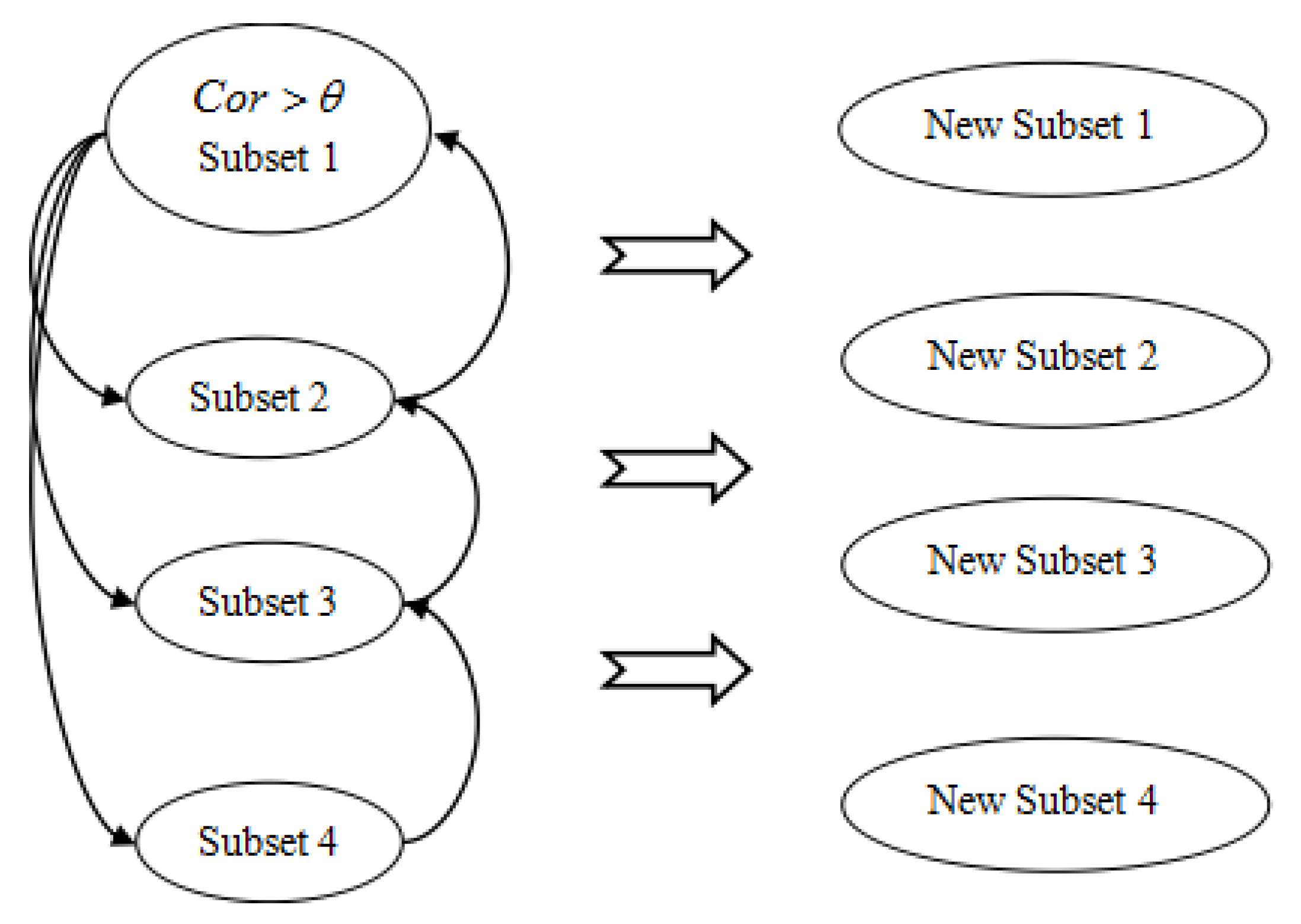If that exists, output the result. If not, select the feature of the highest correlation coefficient from the subset with the maximum fitness and the next subset, and put it into the current set, and then enter a new iteration (Note: the same feature are not allowed in the same subset). The rule is shown in Figure 1.

As shown above, assuming the set of existing subsets is $S_i,i=1,2,3,4$, all the subsets are substituted into the model using the FA algorithm to calculate the fitness function $fitness(i),i=1,2,3,4$ corresponding to each subset, and sorted in descending order:

$$fitness(1)>fitness(2)>fitness(3)>fitness(4)$$

If all the subsets are not up to the expected condition, select the feature of the highest correlation coefficient and put it into the Subset 1 to form the New Subset 1. Then, select the feature of the highest correlation coefficient from the Subset 1 with the maximum fitness and the next Subset 3, and put it into the Subset 2 to form the Subset 3, and then repeat the steps until the last group of New Subset 4 is finished. Finally, put all the new subsets into the next iteration until the expected condition is satisfied, and then output the result.

3. Weighted Least Square Support Vector Regression Model

3.1. Basic Theory of LSSVM

LSSVM is an extension of the support vector machine. It transfers the input vector into high dimensional space through nonlinear casting and constructs the optimal decision surface, and then turns the arithmetic of SVM inequalities into equations calculation according to the risk minimization principle.

Given that a set of data $T={\left\{\left(x_i,y_i\right)\right\}}_{i=1}^N$, in which $x_i$ is input vector, $y_i$ is the expected output, and $N$ is total number of sample. The regression model of the sample is:

$$y\left(x\right)={\mathit{w}}^T·\mathsf{\phi }\left(x\right)+b$$

(9)

where $\mathsf{\phi }(\ast )$ represents casting the training data to a high dimensional space; $w$ is the weighted vector; $b$ is the bias.

For LSSVM, the optimization problem can be transformed into:

$$\min \frac{1}{2}{\mathit{w}}^{\mathit{T}}\mathit{w}+\frac{1}{2}\mathsf{\gamma }{\displaystyle \sum _{i=1}^N{\mathsf{\xi }}_i^2}$$

(10)

$${s·ty}_i=w^T\mathsf{\phi }\left(x_i\right)+b+{\mathsf{\xi }}_i,i=1,2,3,\cdots N;$$

(11)

where $\mathsf{\gamma }$ is the punishment coefficient for balancing the complexity and accuracy; ${\mathsf{\xi }}_i$ is the estimated error. To solve the above equations, it must be transferred to the Lagrange function and this issolved in Section 3.3.

3.2. Improvement of LSSVM

(1) Horizontal weighted input vectors

The mode of multi-inputs and single output is always emerging in the icing forecasting task. The value of the input vector $x_i$ is distributed along with the time and the influence of the actual value of the icing thickness at different times and can be reflected by the weighted processing. Therefore, the input vector can be weighted according to the following formula:

$${\widehat{x}}_i=x_{ki}\cdot \mathsf{\delta }{\left(1-\mathsf{\delta }\right)}^{n-i},k=1,2,\cdots ,l$$

(12)

where ${\widehat{x}}_i$ is the weighted vector; $x_{ki}$ is the original vector; $k$ is the dimension number of input vectors; $\mathsf{\delta }$ is a constant.

(2) Vertical weighted training data set

The predicted value of ice forecasting is not only related to the elements in the input vector, but also with the sample group. This correlation is reflected as: near distance samples have a great influence on the prediction, but the distant samples have little effect on the forecasting. So it is necessary to reduce the impact of near distance samples on the prediction model by using different membership values of the current icing thickness. The membership values can be calculated by using the linear membership ${\mathsf{\mu }}_i$, and the equation is as follows:

$${\mathsf{\mu }}_i=\mathsf{\beta }+i(1-\mathsf{\beta })/N,0\le {\mathsf{\mu }}_i\le 1$$

(13)

where ${\mathsf{\mu }}_i$ is the value of membership; $\mathsf{\beta }$ is a constant between 0 and 1; $i=1,2,\cdots ,N$. The input sample set can be transformed into:

$$T=\left\{\begin{array}{cccc}\left(x_1,y_1,{\mathsf{\mu }}_1\right)& \left(x_2,y_2,{\mathsf{\mu }}_2\right)& \cdots & \left(x_N,y_N,{\mathsf{\mu }}_N\right)\end{array}\right\}$$

(14)

The determination value of $\mathsf{\beta }$ directly impacts the performance of LSSVM, thus the value of $\mathsf{\beta }$ can be obtained by calculating the gray correlation coefficient. The gray correlation coefficient is calculated as follows:

$$r\left(x_0(k),x_i(k)\right)=\frac{{\Delta }_{ki}(\min )+\mathsf{\rho }{\Delta }_{ki}(\max )}{{\Delta }_{ki}+\mathsf{\rho }{\Delta }_{ki}(\max )}$$

(15)

$${\Delta }_{ki}=\left|x_0(k)-x_i(k)\right|\mathsf{\rho }\in [0,1]$$

(16)

$${\mathsf{\beta }}_i={\displaystyle \sum _{k=1}^{N}r\left(x_0(k),x_i(k)\right)}$$

(17)

Considering the multi-inputs and single output of icing forecasting, this paper will let $x_0=Y,Y=\left\{y_1,y_2,\cdots ,y_N\right\}$.

3.3. Weighted LSSVM

Apply the improvements of Section 3.2 into LSSVM to form a weighted LSSVM, thus the objective function can be described as follows:

$$min\frac{1}{2}{\mathit{w}}^{\mathit{T}}\mathit{w}+\frac{1}{2}\mathsf{\gamma }{\displaystyle \sum _{i=1}^N{\mathsf{\mu }}_i{\mathsf{\xi }}_i^2}$$

(18)

$${s·ty}_i={\mathit{w}}^T\mathsf{\phi }\left(x_i\right)+b+{\mathsf{\xi }}_i,i=1,2,3,\cdots N;$$

(19)

In order to solve the above problem, the Lagrange function is established:

$$L\left(\mathit{w},b,{\mathsf{\xi }}_i,{\mathsf{\alpha }}_i\right)=\frac{1}{2}{\mathit{w}}^{\mathit{T}}\mathit{w}+\frac{1}{2}\mathsf{\gamma }{\displaystyle \sum _{i=1}^N{{\mathsf{\mu }}_i\mathsf{\xi }}_i^2}-{\displaystyle \sum _{i=1}^N{\mathsf{\alpha }}_i}\left[{\mathit{w}}^T\mathsf{\phi }\left({\mathrm{x}}_{\mathrm{i}}\right)+b+{\mathsf{\xi }}_i-y_i\right]$$

(20)

where ${\mathsf{\alpha }}_i$ is Lagrange multiplier. Each variable of the function is derivated, and is made to zero:

$$\{\begin{array}{l}\frac{\partial L}{\partial \mathit{w}}=0\to \mathit{w}={\displaystyle \sum _{i=1}^N{\mathsf{\alpha }}_i\mathsf{\phi }\left(x_i\right)}\\ \frac{\partial L}{\partial b}=0\to {\displaystyle \sum _{i=1}^N{\mathsf{\alpha }}_i=0}\\ \frac{\partial L}{\partial \mathsf{\xi }}=0\to {\mathsf{\alpha }}_i=\mathsf{\gamma }{\mathsf{\mu }}_i{\mathsf{\xi }}_i\\ \frac{\partial L}{\partial \mathsf{\alpha }}=0\to {\mathit{w}}^T+b+{\mathsf{\xi }}_i-y_i=0\end{array}$$

(21)

Eliminate $\mathit{w}$ and ${\mathsf{\xi }}_{\mathit{i}}$, and transform it into the following problem:

$$\left[\begin{array}{cc}0& {\mathit{e}}_n^T\\ {\mathit{e}}_n& \mathrm{\Omega }+{\mathsf{\gamma }}^{-1}{\mathsf{\mu }}^{-1}\cdot I\end{array}\right]\cdot \left[\begin{array}{c}b\\ a\end{array}\right]=\left[\begin{array}{c}0\\ y\end{array}\right]$$

(22)

where $\mathrm{\Omega }={\mathsf{\phi }}^T\left(x_i\right)\mathsf{\phi }\left(x_i\right)$, ${\mathit{e}}_n={\left[1,1,\mathrm{...},1\right]}^T$, $\mathsf{\alpha }=\left[{\mathsf{\alpha }}_1,{\mathsf{\alpha }}_2,\mathrm{...},{\mathsf{\alpha }}_n\right]$, $y={\left[y_1,y_2,\mathrm{...},y_n\right]}^T$

Solve the above equations and obtain the following equation:

$$y\left(x\right)={\displaystyle \sum _{i=1}^N{\mathsf{\alpha }}_{i}K\left({\mathit{x}}_{\mathit{i}},\mathit{x}\right)}+b$$

(23)

where $K\left({\mathit{x}}_i,\mathit{x}\right)$ is the kernel function.

This paper uses the wavelet kernel function [31] $K(x_i,x)={\displaystyle \prod _{i=1}^N\mathsf{\psi }\left(\frac{x_i-x_i^{\prime }}{{\mathsf{\sigma }}_i}\right)}$ in $y\left(x\right)$:

$$y\left(x\right)={\displaystyle \sum _{i=1}^N{\mathsf{\alpha }}_i{\displaystyle \prod _{i=1}^N\mathsf{\psi }(\frac{x_i-x_i^{\prime }}{{\mathsf{\sigma }}_i})}}+b$$

(24)

$$\mathsf{\psi }(x)=\cos (1.75x)\cdot \exp (\frac{-x^2}{2})$$

(25)

The reason why the wavelet kernel function is used to replace the Gaussian kernel is mainly based on the following considerations [12]: (1) the wavelet kernel function has the fine characteristic of progressively describing the data, and using the SVM of the wavelet kernel function can approximate any function with high accuracy while the traditional Gaussian kernel function cannot; (2) the wavelet kernel functions are orthogonal or nearly orthogonal, and the traditional Gaussian kernel functions are relevant, even redundant; (3) the wavelet kernel function has multi-resolution analyzing ability for wavelet signals, so the nonlinear processing capacity of the wavelet kernel function is better than that of the Gaussian kernel function, which can improve the generalization ability of the support vector machine regression model.

Finally, the regression equation of W-LSSVM is obtained as:

$$y\left(x\right)={\displaystyle \sum _{i=1}^N{\mathsf{\alpha }}_i{\displaystyle \prod _{i=1}^N\{\cos [\frac{1.75(x_i-x_i^{\prime })}{{\mathsf{\sigma }}_i}]\cdot \exp [\frac{-{(x_i-x_i^{\prime })}^2}{2}]\}}}+b$$

(26)

4. Experiment Simulation and Results Analysis

4.1. Weighted LSSVM Based on FA

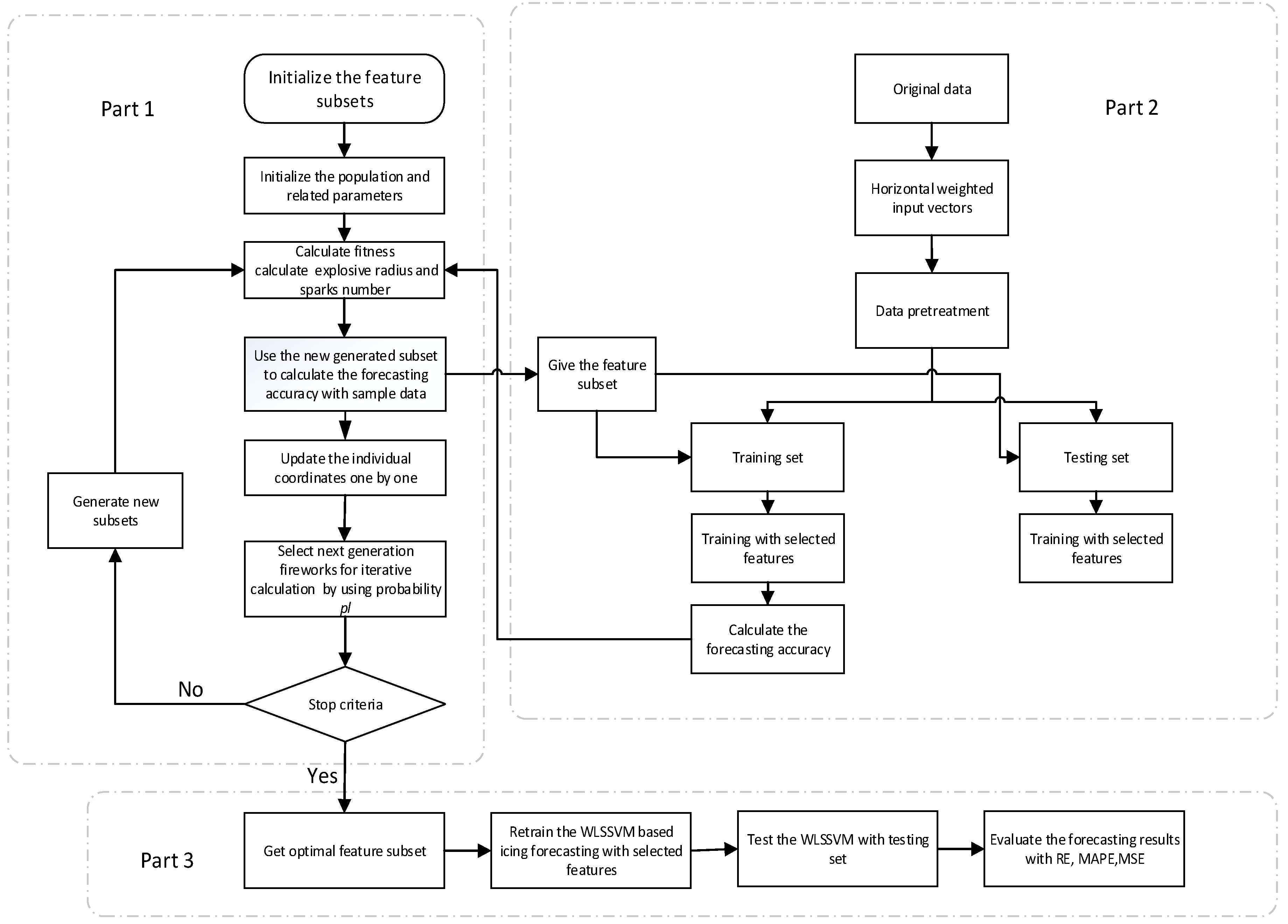
The process of using FA for feature selection and W-LSSVM for icing forecasting is shown in Figure 2. As we can see, the proposed icing forecasting system mainly includes three parts: FA based feature selection (Part 1), W-LSSVM based icing forecasting (Part 2), and W-LSSVM based retraining and testing (Part 3). If the established feature subset of each firework cannot reach the required value, it will return the process and continue to build the feature subset until finding the best feature subset. So in the proposed icing forecasting system, the purpose of Part 1 is to make iterative optimization and count the number of selected features of each firework; and the aim of Part 2 is to calculate the accuracy of each firework; then we can obtain the fitness value of each firework by calculating formula (7). Finally, we retrain the W-LSSVM and evaluate the testing set by adopting the best subset in Part 3.

Step 1: Except for the historical icing thickness data, we select the temperature, humidity, wind speed, wind direction, sunlight intensity, air pressure, altitude, condensation level, line direction, line suspension height, load current, rainfall, and conductor temperature as the candidates influencing the features of icing thickness. Besides, the former $T-i$’s temperature, humidity, wind speed ($i=1,2,4$) are also selected as the major influencing factors of icing forecasting. The initial candidate features are listed in

Table 1. Candidate features table.

$C_1,\cdots ,C_4$	$T_{t-i},i=0,1,2,4$, expresses temperature when time is $t-i$.
$C_5,\cdots ,C_8$	$H_{t-i},i=0,1,2,4$, expresses humidity when time is $t-i$.
$C_9,\cdots ,C_{12}$	$W{S}_{t-i},i=0,1,2,4$, expresses wind speed when time is $t-i$.
$C_{13}$, $C_{14}$, $C_{15}$	$WD$ expresses wind direction, $S$ expresses sunlight intensity, $AP$ expresses air pressure.
$C_{16}$, $C_{17}$, $C_{18}$	$AL$ expresses altitude, $C$ expresses condensation level, $LD$ expresses line direction.
$C_{19}$, $C_{20}$	$LSH$ expresses line suspension height, $LC$ represents load current.
$C_{21}$, $C_{22}$	$R$ expresses rainfall, $CT$ expresses conductor temperature.

. In this case, the two features of rainfall and conductor temperature are directly eliminated, because most of the data points of them are 0 and have little correlation with icing thickness. In the fireworks algorithm, each particle represents a feature subset, the subset should be initialized by using the rules as shown in Section 2. Besides, some parameters of FA should be initialized, such as population size $PopNum$, maximum iterative number $Maxgen$, the constant determining the number of sparks $M$, the constant determining the explosion radius $\widehat{R}$, the upper and lower limits of the individual searching range of fireworks $V_{up}$ and $V_{down}$. After the above preparation, apply the candidate features data into the feature selection process of FA, and obtain the optimal feature subset.

Step 2: Apply the feature subset of each iteration to W-LSSVM, and the predicted accuracy of the feature subset $r(i)$ will be calculated by learning the training samples. Then, the fitness function value of each iteration process $fitness(i)$ can be calculated. By comparing the value of each particle’s fitness function, the optimal subset $subset(i)$ is obtained. If the stop criteria is not satisfied in this iteration, the new initial feature subset $Newsubset(i)$, obtained by the subset selection rules, enters a new round of iteration until the final optimal subset is obtained. It is should be noted that parameters in the W-LSSVM model should be initialized. $\mathsf{\gamma }$, $\mathsf{\sigma }$ are assigned random values.

Step 3: Use the final optimal feature subset to retrain the W-LSSVM based on the icing thickness data. Parameters determination of W-LSSVM has impact on the training and learning ability and has a strong relationship with the forecasting accuracy, so the parameters $\mathsf{\gamma },\mathsf{\sigma }$ of W-LSSVM should be optimized by the fireworks algorithm to find the optimal parameters to improve the forecasting accuracy, rather than be directly subjectively defined.

4.2. Data Selection and Pretreatment

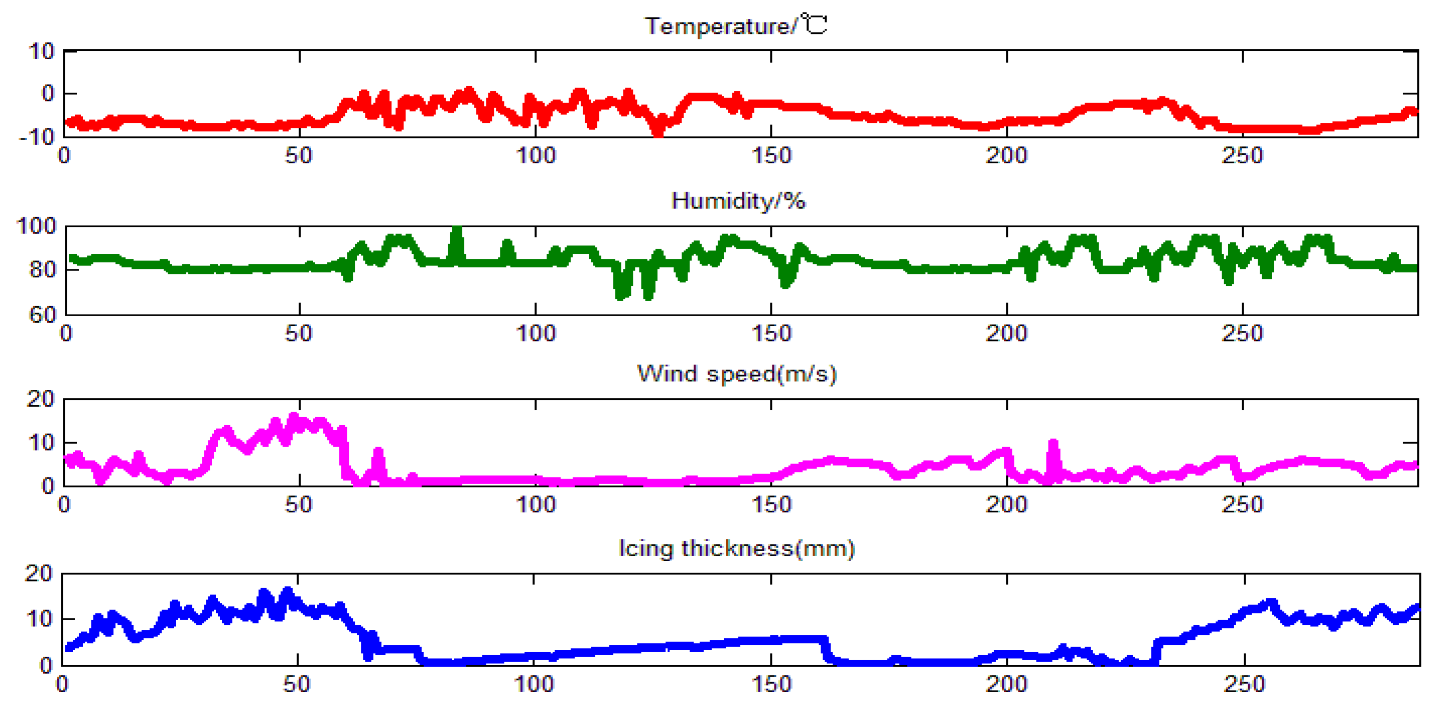
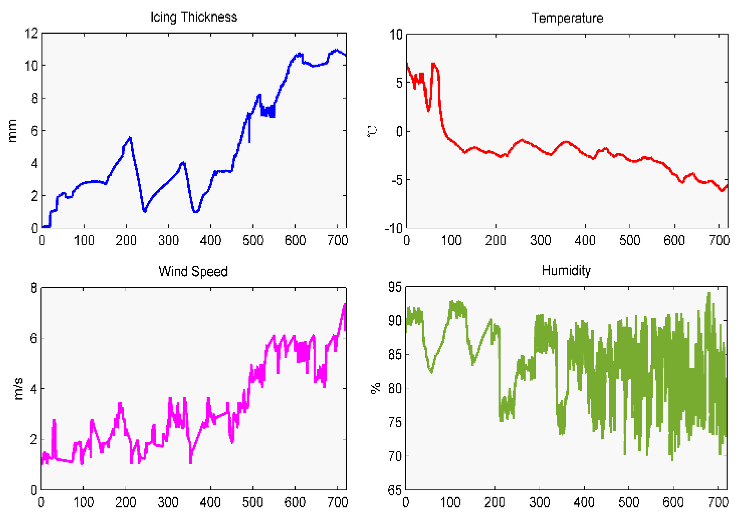
Data are chosen from the data monitoring center of the key laboratory of anti-ice disaster. A 500 kV overhead transmission line called “Zhe-Ming line”, located in Hunan Province, China, is chosen as the real-world case study. The icing data points are collected every fifteen minutes from 0:00 on 4 January 2015 to 11:45 on 11 January 2015, which total up to 720 data points, as shown in Figure 3. The former 576 data points are used as a training sample, and the last 144 as testing sample. Furthermore, the main micro-meteorology data, including temperature, humidity, and wind speed, are shown in Figure 3.

Hunan Province is located in the middle and lower reaches of the Yangtze River and in the south of the Dongting Lake, surrounded by mountains on three sides; the Xiangzhong basin mainly includes hills, mounds, and valley alluvial plains. The terrain is very conducive for winter strong cold air to sweep from the North, and the Nanling stationary front is formed at the confluence of the cold air and the South China Sea subtropical warm air at the north slope of the Nanling mountains. In the areas covered with the stationary front, the super-cooled water in the condensation layer is very unstable, and extremely easy to adhere to relatively cold hard objects such as wires to form rime and glaze. In 2008, Hunan power grid suffered severe freezing damage, which caused many incidents such as tower collapse, line breakage, ice flash, tripping, etc., leading to a large scale blackout disaster. The freezing time, covering area and icing conditions of this damage had been the most serious since 1954. Therefore, the high voltage transmission lines in Hunan Province have been selected as a case study, which has a certain universality.

Before the program running, the historical micro-meteorology data and icing thickness data must be pre-processed to ensure the requirements of the W-LSSVM are met. First, each input should be weighted by the formula (12), which can reflect the forecasting differences between actual icing values and predictive values. Second, to avoid the scaling problem, the sample data should be scaled to the range [0, 1] by using their maximum and minimum values. Finally, it should be noted that the predicted values must be re-scaled back by using the reverse formula in order to guarantee the convenience and maneuverability for the results analysis. The scaled formula of sample data is shown as follows:

$$Z=\left\{z_i\right\}=\frac{y_i-y_{\min }}{y_{\max }-y_{\min }}i=1,2,3,\mathrm{...},n$$

(27)

where $y_{\max }$ and $y_{\min }$ are the maximum and minimum value of sample data, respectively.

4.3. Fireworks Algorithm for Feature Selection

In this section, we use the fireworks algorithm to obtain the final optimal feature subset. The environment used for feature selection includes a Matlab R2013a, a self-written Matlab program, and a computer with the Intel(R) Core(TM)2Duo CPU, 3GB RAM and the Windows 7 Professional operation system. The parameters of fireworks algorithm are set as follows: the maximum iteration number $Maxgen=500$, the population size $PopNum=30$, the constant determining the number of sparks $M=100$, the constant determining the explosion radius $\widehat{R}=150$, the upper and lower limits of the individual searching range of fireworks are $V_{up}=512$ and $V_{down}=-512$ respectively. The parameters of W-LSSVM are chosen as follows: $\mathsf{\gamma }=23.698$, $\mathsf{\sigma }=5.123$.

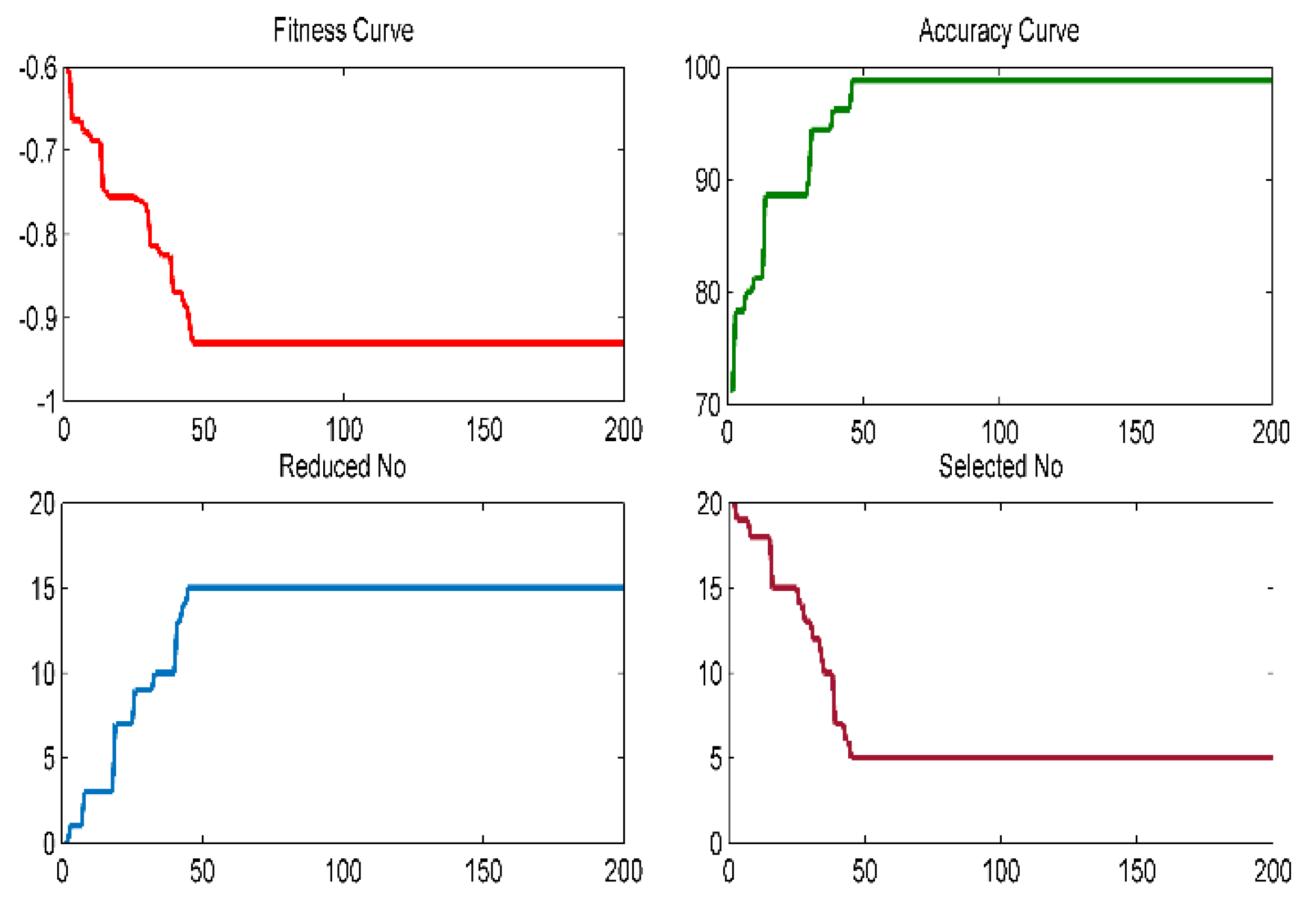
Figure 4 is the iterative process curve of the fireworks algorithm for the sample data. As shown in the figure, the fitness curve describes the best fitness value which is obtained by the FA model at each iteration; the accuracy curve is the value which is calculated by the W-LSSVM model at different iterations; the reduced No is the number of eliminated features in the process of convergence; and the selected No is the number of obtained features in every iteration with the new method. As we can see from Figure 4, the optimal fitness value is −0.93, which is found by FA when the iterative number reaches 46. In the 46th iteration, the prediction accuracy based on the training sample meets the best value of 98.8%; which means the machine learning of the W-LSSVM achieves the best value and obtains the highest predictive accuracy in the training sample data. Furthermore, the number of selected features is stable when the iterative number is 46, and we can see that 15 features are eliminated from the original 20 features due to the low coefficient between these 15 candidate features and the icing thickness. The final selected features for the sample are temperature, humidity, wind speed, sunlight intensity, and air pressure, respectively.

4.4. W-LSSVM for Icing Forecasting

Before all calculations are carried out, it is necessary to state that the methods presented in this paper do not exhibit any uncertainty in the prediction process. This is also the next important work in our future research.

After obtaining the final features of the data, the inputs into the W-LSSVM to retrain and test the data are applied. In this paper, Matlab is used to run the self-written program and calculate the results; it is worth noting that the wavelet kernel function is chosen as the kernel function of W-LSSVM, and the parameters of W-LSSVM are obtained by using FA to optimize them. Parameters of fireworks algorithm are set as shown in Section 4.3; through the calculation, the parameters of W-LSSVM are chosen as follows: $\mathsf{\gamma }=42.4756$, $\mathsf{\sigma }=18.8812$.

In order to prove the performance of the proposed forecasting model for icing thickness, three well-known icing forecasting models including SVM (support vector machine), BPNN (BP neural networks), and MLRM (multi-variable linear regression model) are also applied to the data-set described in Section 4.2.

In the single SVM forecasting model, three input vectors, including temperature, humidity, and wind speed, can be regarded as support vectors of the SVM model. Additionally, the parameters of $C,\mathsf{\sigma },\mathsf{\epsilon }$ are obtained by cross validation on the former 576 training data. Through the training calculation, the parameters are chosen as follows:

$$C=10.913,\mathsf{\epsilon }=0.0012,\mathsf{\sigma }=2.4532.$$

In the BPNN icing forecasting model, the number of input layers, hidden layers, and output layers are 5, 7, and 1 respectively. The Sigmoid function is selected as the transfer function. The maximum permissible error of model training is 0.001, and the maximum training time is 5000.

Furthermore, this paper uses the relative error (RE), mean absolute percentage error (MAPE), and root mean square relative error (RMSE) as the final evaluation indicators:

$$RE=\frac{y(i)-\widehat{y}(i)}{y(i)}\times 100\%$$

(28)

$$MAPE=\frac{1}{N}{\displaystyle \sum _{i=1}^N\left|\frac{y(i)-\widehat{y}(i)}{y(i)}\right|}\times 100\%$$

(29)

$$RMSE=\sqrt{\frac{1}{N}{\displaystyle \sum _{i=1}^N{(\frac{y(i)-\widehat{y}(i)}{y(i)})}^2}}$$

(30)

where $y(i)$ is the original icing thickness value, and $\widehat{y}(i)$ is the predictive value.

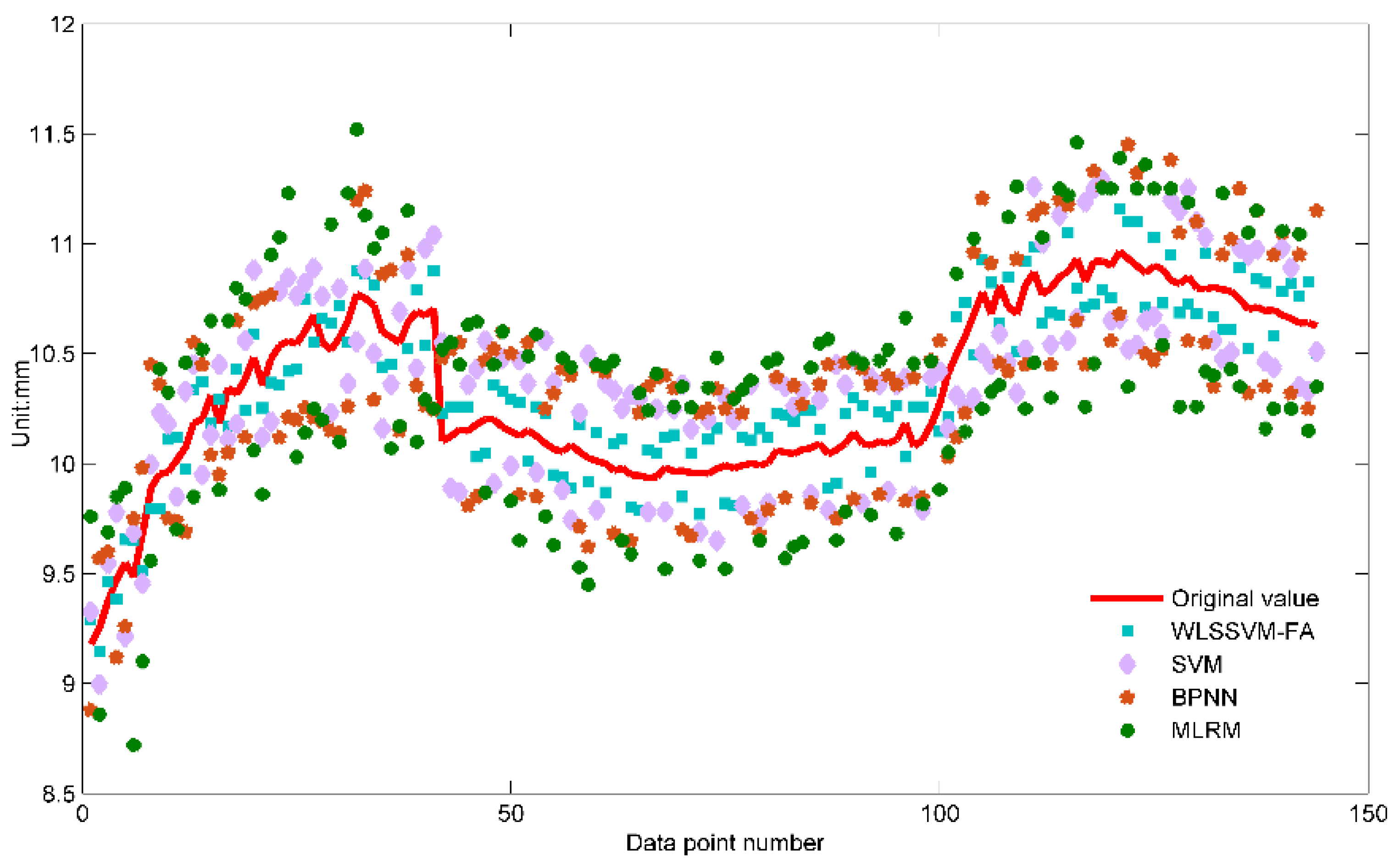
All the icing thickness forecasting value with the BP, SVM, W-LSSVM-FA, and MLRM models are shown in Figure 5, part of which are given in

Table 2. The forecasting values and errors of each model.

Time Point	Actual Value (mm)	BPNN		SVM		W-LSSVM-FA		MLRM
		Forecast Value (mm)	Error	Forecast Value (mm)	Error	Forecast Value (mm)	Error	Forecast Value (mm)	Error
T07-00	10.900	10.47	−3.95%	10.67	−2.11%	11.03	1.19%	11.25	3.21%
T07-15	10.89	10.52	−3.36%	10.59	−2.72%	10.73	−1.43%	10.54	−3.18%
T07-30	10.83	11.38	5.05%	11.20	3.39%	10.949	1.08%	11.25	3.85%
T07-45	10.82	11.05	2.14%	11.15	3.06%	10.686	−1.22%	10.26	−5.16%
T08-00	10.85	10.56	−2.67%	11.25	3.69%	10.725	−1.15%	11.19	3.12%
T08-15	10.80	11.10	2.79%	11.10	2.79%	10.682	−1.08%	10.26	−4.99%
T08-30	10.79	10.55	−2.25%	11.03	2.20%	10.956	1.51%	10.42	−3.45%
T08-45	10.80	10.35	−4.19%	10.56	−2.25%	10.666	−1.27%	10.4	−3.73%
T09-00	10.79	10.95	1.47%	10.48	−2.92%	10.612	−1.67%	11.23	4.06%
T09-15	10.78	11.02	2.20%	10.51	−2.57%	10.612	−1.58%	10.43	−3.27%
T09-30	10.75	11.25	4.66%	10.98	2.15%	10.893	1.34%	10.35	−3.71%
T09-45	10.70	10.32	−3.57%	10.95	2.32%	10.525	−1.66%	11.05	3.25%
T10-00	10.71	11.15	4.09%	10.98	2.45%	10.84	1.19%	11.15	4.09%
T10-15	10.70	10.35	−3.22%	10.47	−2.15%	10.823	1.20%	10.16	−5.00%
T10-30	10.70	10.95	2.34%	10.44	−2.46%	10.58	−1.12%	10.25	−4.20%
T10-45	10.68	11.05	3.51%	10.98	2.86%	10.783	1.01%	11.06	3.61%
T11-00	10.66	10.32	−3.19%	10.89	2.16%	10.82	1.50%	10.25	−3.85%
T11-15	10.64	10.95	2.91%	10.35	−2.73%	10.76	1.12%	11.05	3.80%
T11-30	10.64	10.25	−3.68%	10.33	−2.93%	10.826	1.73%	10.15	−4.62%
T11-45	10.63	11.15	4.94%	10.51	−1.09%	10.503	−1.15%	10.35	−2.59%
MAPE	-	-	3.23%	-	2.59%	-	1.35%	-	4.06%
RMSE	-	-	3.31%	-	2.68%	-	1.38%	-	4.16%

BPNN: BP Neural Networks; SVM: Support Vector Machine; MLRM: Multi-Variable Linear Regression Model; MAPE: Mean Absolute Percentage error; RMSE: Root Mean Square Relative Error.

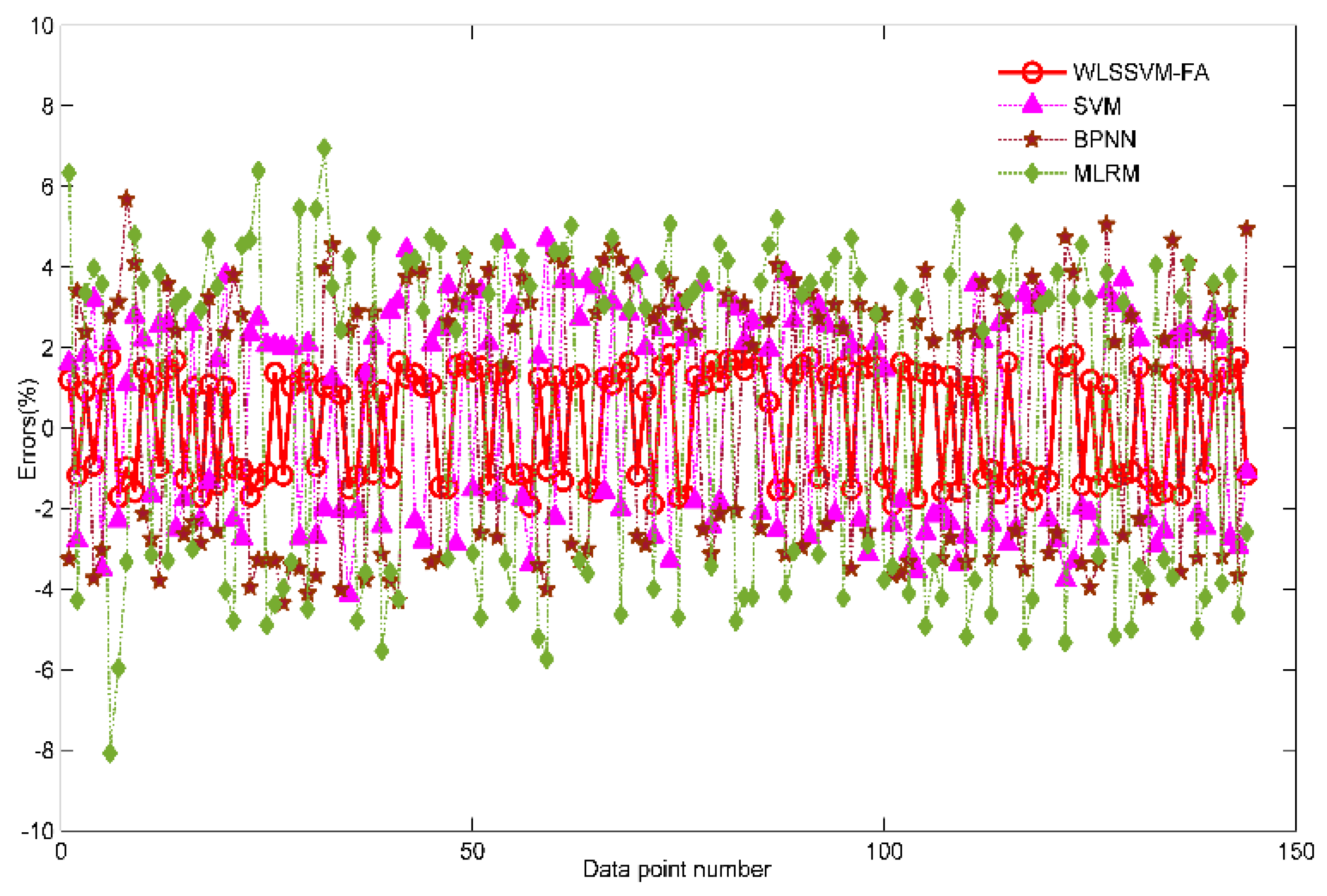
. In addition, Figure 6 gives the forecasting errors with these models. Based on the above results, several patterns are observed.

Firstly, the maximum and minimum gap between original icing value and forecasting value are captured from Figure 5. In the MLRM model, the maximum gap is 0.77 mm, and the minimum gap is 0.25 mm. In the BPNN model, the maximum and minimum gaps are 0.56 mm and 0.16 mm, respectively. Both values of BPNN are smaller than that of MLRM, which indicates that the forecasting accuracy of BPNN is much more precise. In the single SVM model, the maximum and minimum gaps are 0.47 mm and 0.11 mm, respectively. The deviation between the maximum and minimum gaps of the single SVM model is 0.36 mm, which is smaller than that of BPNN and MLRM; this result demonstrates that the SVM icing forecasting model is much more stable than that of BPNN and MLRM. In the proposed W-LSSVM-FA model, the maximum gap is only 0.2 mm and the minimum gap is only 0.064 mm. Compared with the other three models, both values of W-LSSVM-FA are smaller and the deviation between the maximum and minimum gap is 0.136 mm, which is also smaller than that of SVM, BPNN, and MLRM. This illustrates that the proposed W-LSSVM-FA model has a higher prediction accuracy and stability.

Secondly, the relative errors in these models can be described from Figure 6. In the MLSM model, the maximum and minimum relative errors are 8.07% and 2.42%, respectively; and the fluctuating range of the RE curve is higher. In the BPNN model, the maximum error is 5.68% which is smaller than that of MLSM, and the minimum error is 1.47% which is smaller than that of MLSM; this demonstrates that the forecasting accuracy and the nonlinear fitting ability of BPNN is stronger than that of MLSM. In the single SVM model, the maximum and minimum errors are 4.7% and 1.09%; both values of SVM are superior to that of BPNN and MLRM, and the fluctuating range of the RE curves of the SVM is rather smaller. This again demonstrates the accuracy and the stability of SVM are higher than that of BPNN and MLRM in icing forecasting. In the proposed W-LSSVM-FA model, the maximum and minimum relative errors are 1.94% and 0.64%, respectively. Both of the values are the smallest among BPNN, SVM, and MLRM models. Moreover, the fluctuation of the curve is small, which is superior to the other models. Compared with the other three models, the proposed W-LSSVM-FA icing forecasting model has a higher accuracy and stability. Due to the fact that it performs a great pretreatment on the data with the input vectors weighted and that some redundant factors have been eliminated through the feature selection, the forecasting accuracy is improved, and the machine learning and training ability are relatively strengthened.

Thirdly, the forecasting results can be evaluated by calculating the MAPE and RMSE. As the calculation results are shown, the MAPE values of the W-LSSVM-FA, SVM, BPNN, and MLRM models are 1.35%, 2.59%, 3.23%, and 4.06%, respectively. The proposed W-LSSVM-FA model has a lower error than the other models. The RMSE value is used to evaluate the discrete degree of whole forecasting values of each model. As we see in Table 2, the RMSE values of W-LSSVM-FA, SVM, BPNN, and MLRM are 1.38%, 2.68%, 3.31%, and 4.16%, respectively. The discrete degree of the W-LSSVM-FA icing forecasting model is the lowest; this demonstrates the proposed W-LSSVM-FA model is more stable for the prediction of icing thickness, and it can reduce the redundant influence of irrelevance factors through feature selection.

4.5. Further Simulation

To verify whether the W-LSSVM can bring better results, another representative 500 kV high voltage transmission line, called “Fusha-Ӏ-xian”, was selected to make a comparison of the forecasting results by using the selected features (W-LSSVM-FA method) and original features (only W-LSSVM method). The sample data of “Fusha-Ӏ-xian” were also predicted by BPNN, SVM, MLRM and the results of the five models were also used to make a comparison. The data of “Fusha-Ӏ-xian” are from 12 January 2008 to 25 February 2008, which totally have 287 data groups. Also, part of the original data is shown in Figure 7. The former 247 data points are used as training sample, and the last 40 as testing sample.

In the W-LSSVM-FA model, the FA model is used to select the features. First, initialize the parameters of the FA model: set the maximum iteration number $Maxgen=500$, the number of initial fireworks $PopNum=30$, the sparks number determination constant $M=100$, the explosion radius determination constant $\widehat{R}=150$, and the upper and lower limits of the individual searching range of fireworks are $V_{up}=512$ and $V_{down}=-512$, respectively. 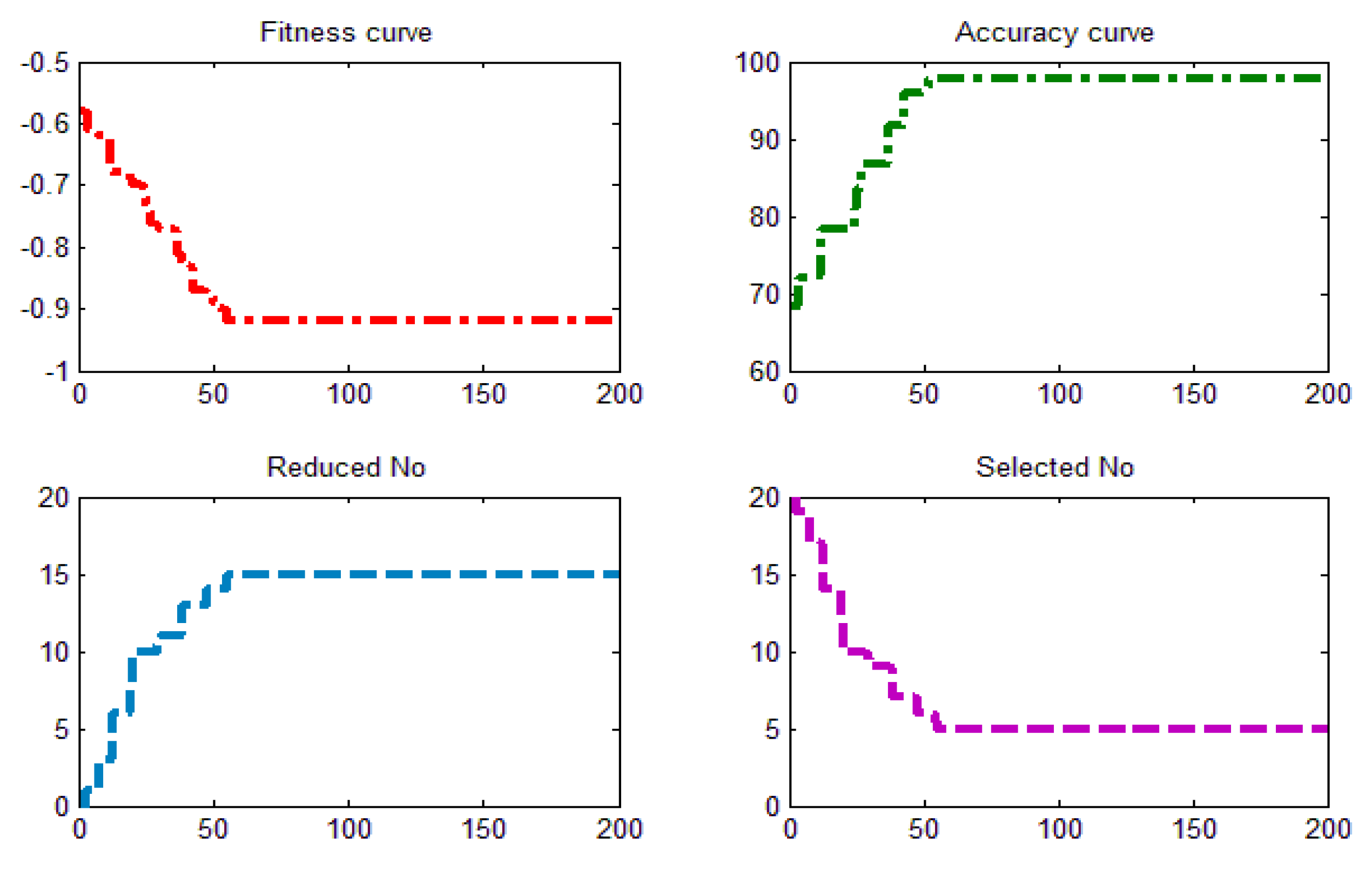Let the border of parameter $\mathsf{\gamma }$ be $[2^{-5},2^{10}]$ and the border of parameter $\mathsf{\sigma }$ be $[2^{-5},2^5]$, respectively. Also, the final selected features are temperature, humidity, wind speed, rainfall, load current, air pressure, and sunlight intensity, respectively. The iterative process curve of the fireworks algorithm for the sample data of “Fusha-I-xian” is shown in Figure 8. As we can see from Figure 8, the optimal fitness value is −0.916, which is found by FA when the iterative number reaches 55. The final selected features for the sample are temperature, humidity, wind speed, wind direction, and sunlight intensity, respectively. The parameters of W-LSSVM-FA are obtained as follows: $\mathsf{\gamma }=56.7841$, $\mathsf{\sigma }=14.7715$. In the W-LSSVM model, the original features are only temperature, humidity, and wind speed. With the method of cross validation, the parameters of W-LSSVM are obtained as follows: $\mathsf{\gamma }=38.9962$, $\mathsf{\sigma }=15.3720$.

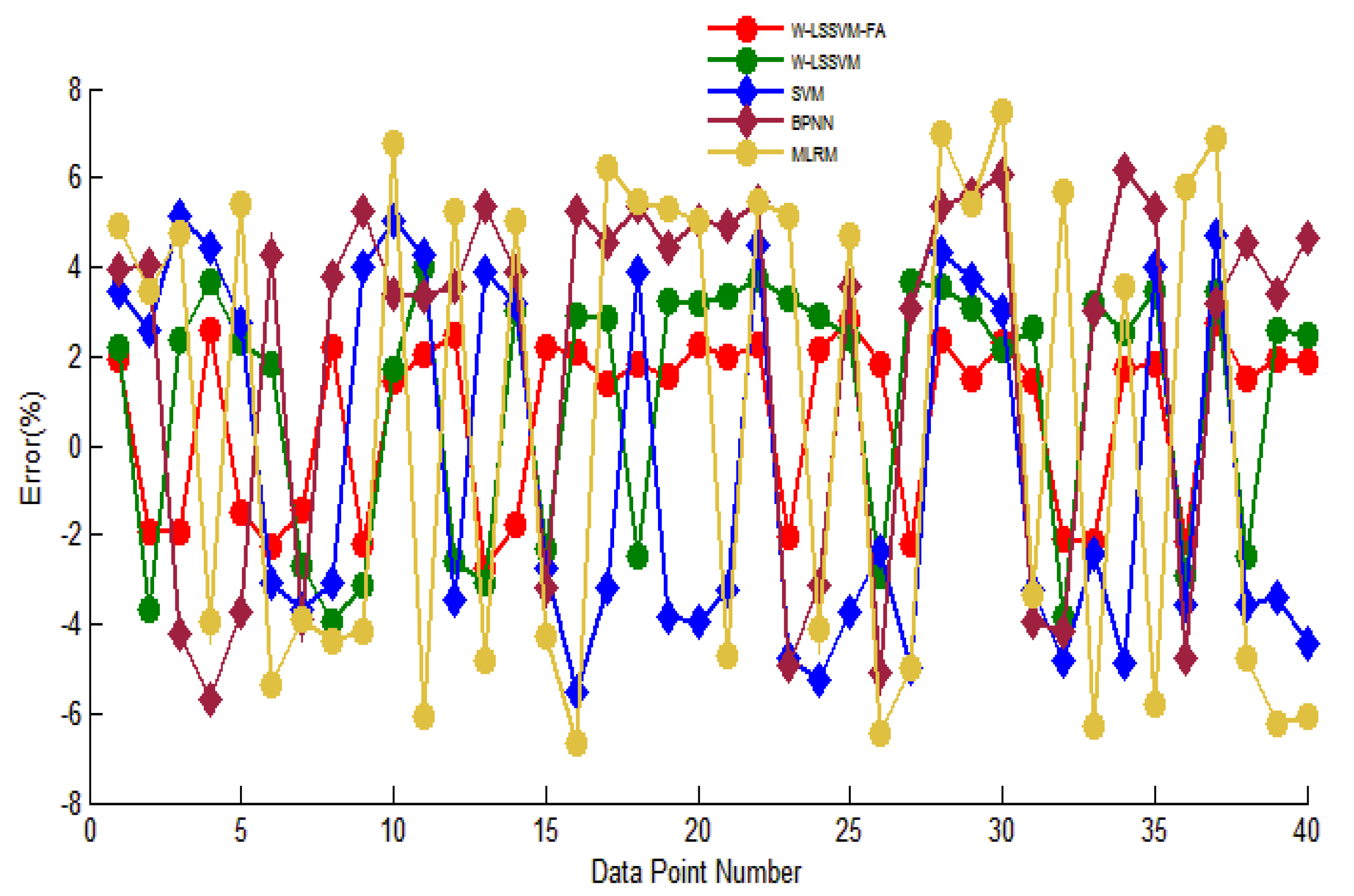
All forecasting results and the relative errors of the five models are shown in Figure 9 and Figure 10, respectively. A part of the forecasting values and errors of five models is listed in

Table 3. Part of the forecasting values and relative errors of each model.

Forecasting Point Number	Actual Value (mm)	W-LSSVM-FA		W-LSSVM		SVM		BPNN		MLRM
		Forecast Value	Error	Forecast Value	Error	Forecast Value	Error	Forecast Value	Error	Forecast Value	Error
1	11.67	11.84	1.46%	11.98	2.66%	11.29	−3.26%	11.21	−3.94%	11.28	−3.34%
2	12.49	12.23	−2.08%	12.01	−3.84%	11.89	−4.80%	11.97	−4.16%	13.2	5.68%
3	11.67	11.42	−2.14%	12.04	3.17%	11.39	−2.40%	12.02	3.00%	10.94	−6.26%
4	10.65	10.83	1.69%	10.92	2.54%	10.13	−4.88%	11.31	6.20%	11.03	3.57%
5	9.80	9.98	1.84%	10.14	3.47%	10.19	3.98%	10.32	5.31%	9.23	−5.82%
6	10.67	10.44	−2.16%	10.36	−2.91%	10.292	−3.54%	10.16	−4.78%	11.29	5.81%
7	10.14	10.42	2.76%	10.49	3.45%	10.62	4.73%	10.46	3.16%	10.84	6.90%
8	11.29	11.46	1.51%	11.01	−2.48%	10.89	−3.54%	11.8	4.52%	10.76	−4.74%
9	12.01	12.24	1.92%	12.32	2.58%	11.6	−3.41%	12.42	3.41%	11.26	−6.24%
10	12.39	12.62	1.86%	12.7	2.50%	11.84	−4.44%	12.97	4.68%	11.64	−6.05%
MAPE	-	-	2.02%	-	2.95%	-	3.85%	-	4.41%	-	5.28%
RMSE	-	-	2.05%	-	3.00%	-	3.94%	-	4.50%	-	5.38%

.

As is shown in Figure 9, the prediction values of W-LSSVM-FA are closest to the original values, this again proves the W-LSSVM-FA model has a higher forecasting accuracy and stability compared with the other four prediction models. The prediction results of W-LSSVM are closer to the original data than that of the SVM, BPNN, and MLRM models, this again reveals that it can improve the nonlinear mapping ability and strengthen the learning ability of the machine through the weighting process of LSSVM.

The MAPE and RMSE values of the five models are shown in Table 3. It can be seen that the proposed W-LSSVM-FA model still has the smallest MAPE and RMSE values, which are 2.02% and 2.05%, respectively. This again reveals the proposed W-LSSVM-FA model has the best performance in icing thickness forecasting. Moreover, the MAPE and RMSE values of W-LSSVM are smaller than that of SVM, BPNN, and MLRM; this demonstrates the W-LSSVM has a higher prediction accuracy and better learning ability by using original features to forecast.

The relative errors can be seen in Figure 10. We can see from the above computation that comparing with the W-LSSVM-FA and W-LSSVM method, the W-LSSVM-FA model has a higher forecast precision. Additionally, in the W-LSSVM model, the relative errors are more fluctuant compared with W-LSSVM-FA; it can also be seen that using the W-LSSVM-FA model to forecast has better stability and accuracy than the W-LSSVM model. This is because it can select different features and remove many unrelated factors that have no or little effect on icing forecasting with the fireworks algorithm optimization. Moreover, the use of feature selection with FA can greatly ensure the integrity of the information for different data characteristics, which makes the prediction accuracy of W-LSSVM-FA much higher. On the contrary, the use of original features to forecast is impossible to ensure information completeness for the different data, which may degrade the prediction precision.

In summary, the proposed W-LSSVM-FA can reduce the forecasting errors between original icing thickness values and predictive values. It can reduce the influence of unrelated noises with feature selection based on the fireworks algorithm. The LSSVM model improves its nonlinear mapping ability with horizontal and vertical weighting, and its training and learning ability is strengthened very well in this way. The numerical experimental results demonstrated the feasibility and effectiveness of the proposed W-LSSVM-FA icing forecasting method.

5. Conclusions

This paper proposes an icing forecasting method of the weighted least square support vector machine (W-LSSVM) based on the Fireworks Algorithm (FA). To use the proposed method, the FA is utilized to make feature selection to eliminate the redundant influence of many uncertain factors in icing forecasting. Considering the specific combination optimization problem based on FA, the initial feature subsets are determined by calculating the correlation coefficient. In order to improve the generalization and learning ability of the algorithm, the LSSVM is improved though horizontal and vertical weighting. After automatically obtaining the inputs, WLSSVM is used to train and test the data. According to the results of simulation for the Zhe-Ming transmission line, the proposed W-LSSVM-FA model can find the optimal feature subsets and achieve the expected accuracy. Furthermore, by comparing it with the three classical icing forecasting models (SVM, BPNN, and MLRM), the proposed W-LSSVM-FA model showed superior performance in terms of RE, MAPE, and RMSE. Therefore, it can be concluded that the proposed model might be an alternative for icing forecasting.