Technical Note

Nonlinear Vibration Response of a Rectangular Tube with a Flexible End and Non-Rigid Acoustic Boundaries

Department of Civil and Architectural Engineering, City University of Hong Kong, Kowloon Tong, Kowloon, Hong Kong
Appl. Sci. 2016, 6(12), 424; https://doi.org/10.3390/app6120424
Submission received: 13 September 2016 / Revised: 2 December 2016 / Accepted: 5 December 2016 / Published: 10 December 2016

Abstract

:
This paper addresses the analysis for the nonlinear vibration response of a rectangular tube with a flexible end and non-rigid acoustic boundaries. The structural–acoustic modal formulations are developed from the Duffing differential equation and wave equation, which represent the large-amplitude structural vibration of a flexible panel coupled with a cavity. This problem considers both non-rigid acoustic boundary and structural cubic nonlinearity. The multi-level residue harmonic balance method is employed for solving the nonlinear coupled differential equations developed in the problem. The results obtained from the proposed method and numerical method are generally in good agreement. The effects of excitation magnitude, tube length, and phase shift parameter, etc., are examined.

1. Introduction

In the well-known acoustic text book [
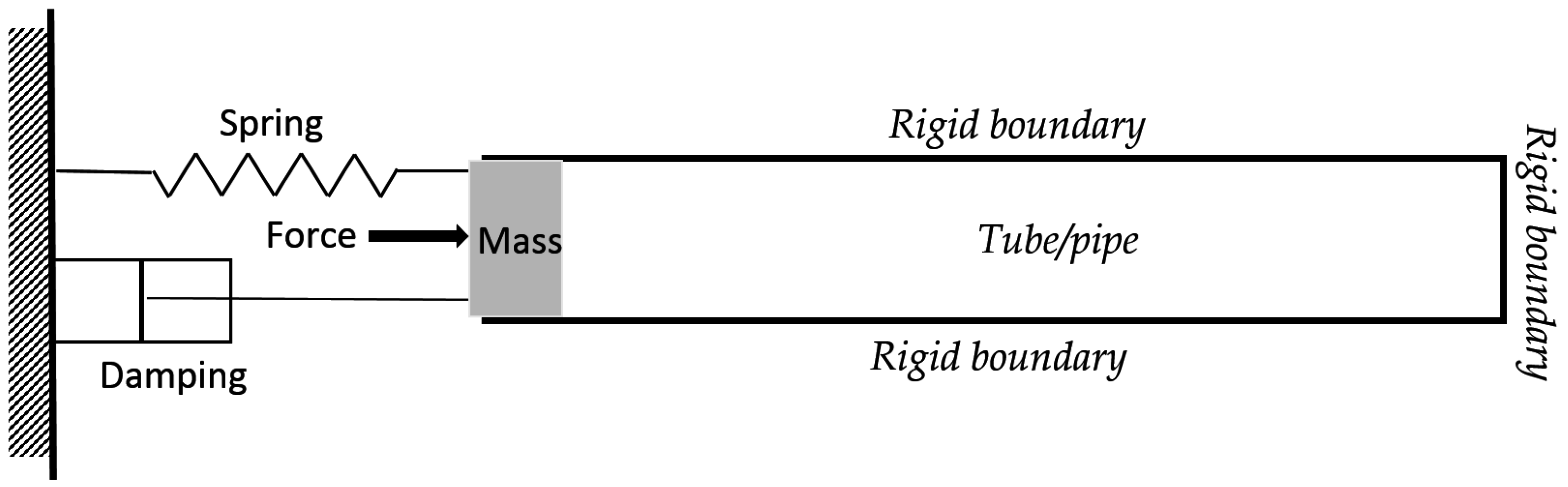
1], an investigation of resonating tube/pipe accounts for the properties of a mechanical driver, which is driven by external excitation (see Figure 1). The driver has its own mechanical impedance. Thus, the system considers the coupling between a linear spring-mass and an internal cavity with rigid acoustic boundaries. Similar to other structural–acoustic problems, the aforementioned problem does not include the structural nonlinearity and non-rigid acoustic boundary.
In practice, there are many engineering problems with structural acoustics, a few examples being: (1) the sound absorption of a panel absorber backed by an air cavity; (2) the vibration response of an aircraft cabin which is a “tube-like” structure enclosing a cavity; and (3) the noise within a rectangular ventilation duct that is formed by thin metal sheets. In these examples, the structures are usually made of thin metal panels and are easily excited to vibrate nonlinearly, and the boundaries of the cavities are not perfectly rigid or fully open. In fact, there have been many research works about linear structural acoustics (e.g., [2,3,4]) or nonlinear vibrations (e.g., [5,6,7,8,9,10,11,12]). However, there are limited works about nonlinear structural–acoustic problems with non-rigid acoustic boundary conditions. This study is a further work of the aforementioned linear structural–acoustic problem in [1]. Thus, this paper would focus on structural nonlinearity and non-rigid acoustic boundary. Moreover, the multi-level residue harmonic balance method, which was developed by Leung and Guo [13] in 2011, and then modified by Hansan et al. [14] in 2013, is employed to solve the nonlinear differential equations, which represent the large-amplitude structural vibration of a flexible panel coupled with a cavity. Table 1 shows the numbers of algebraic equations generated in the multi-level residue harmonic balance method and the classical harmonic method for a cubic nonlinear undamped beam problem. When compared with the classical harmonic balance method, this harmonic balance method requires less computational effort because it requires solving one nonlinear algebraic equation and one set of linear algebraic equations for obtaining each higher-level solution. The solutions from the proposed method are verified by those from the classical harmonic balance method. Parametric studies are performed, and the effects of structural nonlinearity and acoustic boundary condition on the nonlinear vibration responses are investigated in detail.

2. Theory

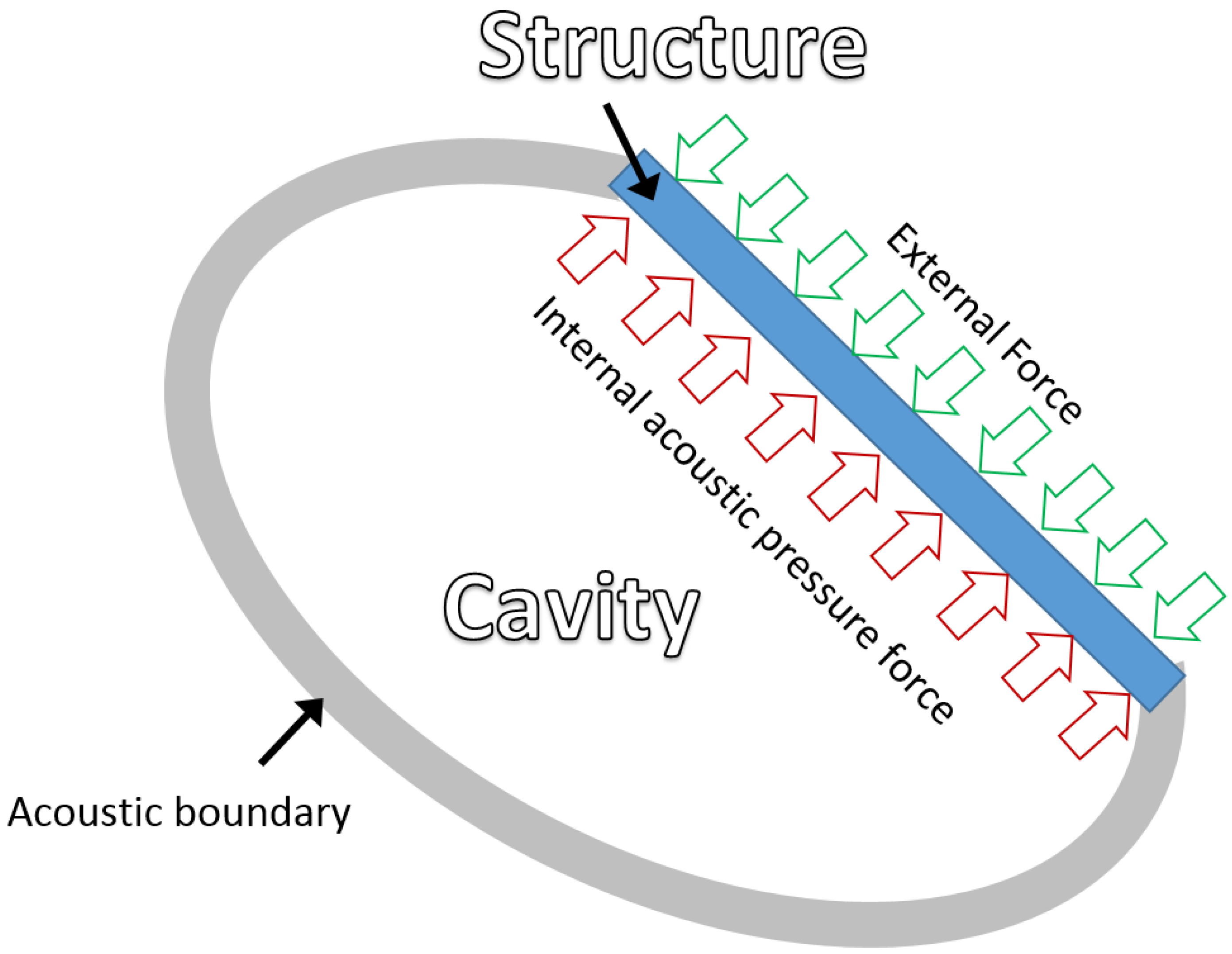
Figure 2 shows the general concept of a structural–acoustic model, in which the structural part is in contact with a finite cavity by physical boundaries. The enclosed volume would induce the acoustic resonant behavior, which is normally modeled using the well-known wave equation [1,2,15,16,17]. This wave equation has been used in numerous applied science/engineering problems for the past few decades. The structural part in the model usually is a plate or a shell, which is subject to an external force and coupled with the internal acoustic pressure within the cavity. The structural vibration directly affects the magnitude of the acoustic pressure acting on the structure. This is so-called structural–acoustic interaction. In the past, many researchers just focused on particular linear/nonlinear plate modellings (e.g., [5,6,7,8,9,10,11,12,18]) or linear structural–acoustic problems with perfectly rigid acoustic boundaries. In this paper, the focuses include the nonlinear structural–acoustic interaction and non-rigid acoustic boundary. 
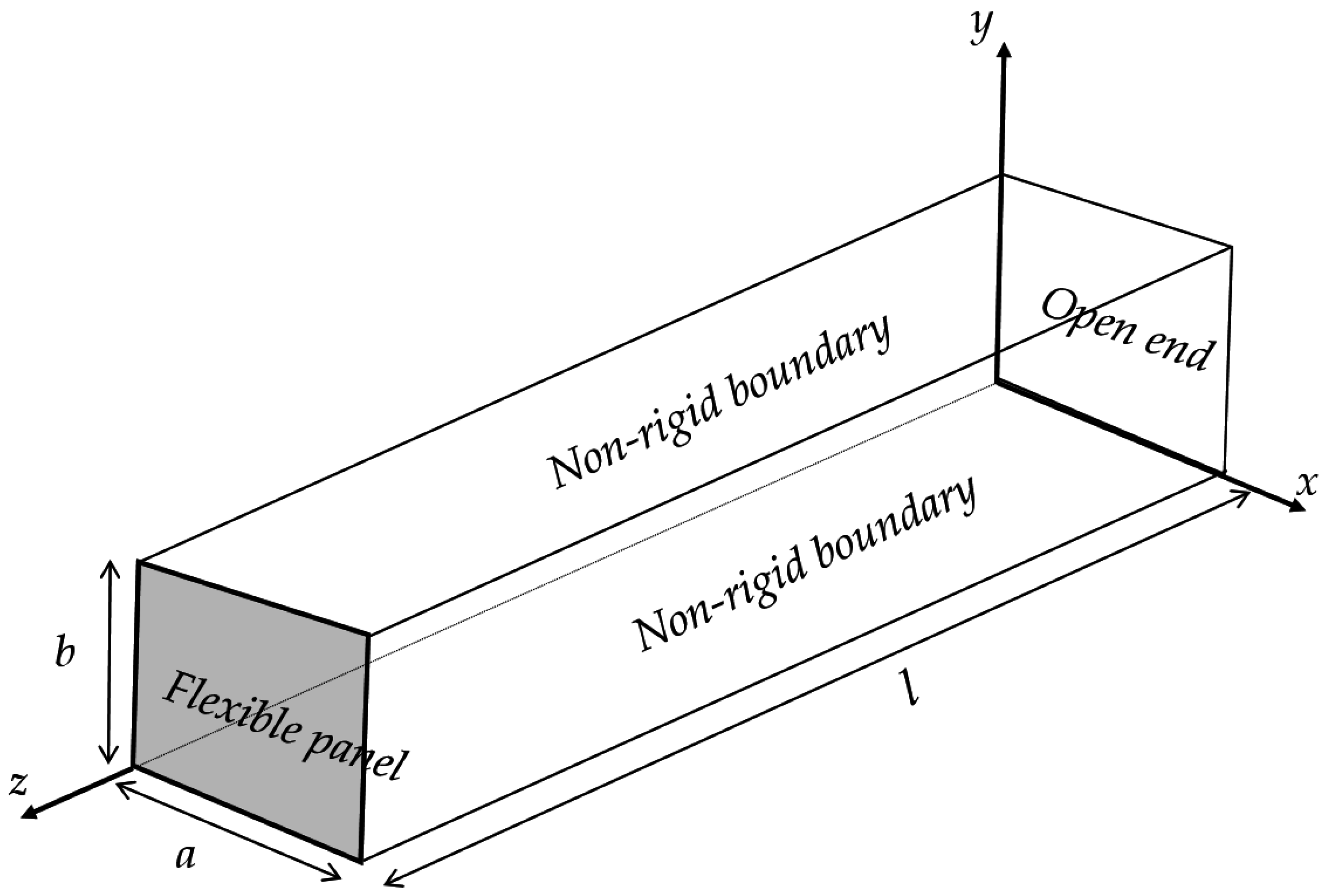
Figure 3 shows the problem considered in this study. The acoustic pressure within the rectangular tube is obtained from the homogeneous wave equation.
2 P h 1 C a 2 2 P h t 2 = 0
where Ph is the h-th harmonic component of the acoustic pressure within the cavity; Ca is the speed of sound.
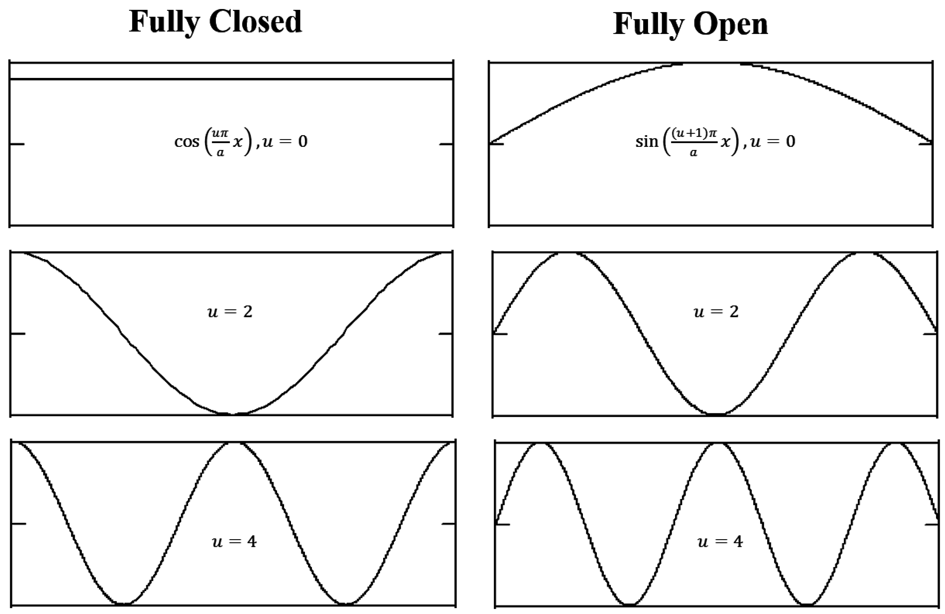
In Figure 4, the boundary conditions of the perfectly rigid and fully open cases at x = 0 and a; y = 0 and b are given by
P h x = P h y = 0 ,   for perfectly rigid
P h = 0 ,   for fully open
According to Equations (2a) and (2b), the acoustic pressure mode shapes of the perfectly rigid and fully open cases are given by
φ u v ( x , y ) = cos ( u π a x ) cos ( v π b y )
φ u v ( x , y ) = sin ( ( u + 1 ) π a x ) sin ( ( v + 1 ) π b y )
where φ u v ( x , y ) is the (u,v) acoustic mode, a and b are the cross-sectional dimensions of the duct, and u and v are the acoustic mode numbers.
Hence, the acoustic pressure mode shape of non-rigid case is defined by
φ u v ( x , y ) = cos ( ( u + η ) π a x η π 2 ) cos ( ( v + η ) π b y η π 2 )
where η = θ 90 ; θ is the phase shift parameter. If η is set as zero in Equation (4), then the acoustic mode shapes become those in the perfectly rigid case.
The boundary conditions at z = l and 0 are given by
P h z = ρ a 2 w c h t 2   at   z = l
P 1 = P o sin ( ω t )   at   z = 0 ,   for   h = 1
P h = 0   at   z = 0 ,   for   h 1
where l is the duct length; ρa = air density; ω = excitation frequency. Note that the external sound pressure at z = 0 is simple harmonic excitation (i.e. no higher harmonic components). P0 = excitation magnitude, γ × Pref; γ is the dimensionless parameter; Pref is the reference pressure level, 102 N/m2. w l h ( x , y , t ) = the hth harmonic component of the nonlinear panel displacement at z = l.
w l h ( x , y , t ) = A h , sin ( t ) ϕ m n ( x , y )
where ϕ m n ( x , y ) = sin ( m π x a ) sin ( n π y b ) = the (m,n) panel mode (it is simply supported). A h , sin ( t ) = A h sin ( h ω t ) ; Ah is the panel vibration amplitude. The total response of the panel is equal to the summation of all harmonic components and given by
w l ( x , y , t ) = h = 1 , 3 , 5 H w l h ( x , y , t ) = h = 1 , 3 , 5 H A h , sin ( t ) ϕ m n ( x , y )
where w c ( x , y , t ) is the displacement response of the panel at z = l. H = the number of harmonic terms. Then, the multi-level residue harmonic balance method is adopted for solving the differential equations and obtaining the unknown panel displacement responses. For simplicity, only the zero, 1st and 2nd level solution procedures (or three harmonic components are considered) are shown here. According to the multi-level residue harmonic balance solution form proposed in [14,19],
A ( t ) = ε 0 A 0 ( t ) + ε 1 A 1 ( t ) + ε 2   A 2 ( t )
where ε is an embedding parameter. Any terms associated with ε0, ε1, ε2 represent those terms considered in the zero, 1st and 2nd level solution procedures respectively. Then, the zero, 1st and 2nd level solutions, A 0 ( t ) , A 1 ( t ) and A 2 ( t ) , are given by
A 0 ( t ) = A 0 1 sin ( ω t )
A 1 ( t ) = A 1 1 sin ( ω t ) + A 1 3 sin ( 3 ω t )
A 2 ( t ) = A 2 1 sin ( ω t ) + A 2 3 sin ( 3 ω t ) + A 2 5 sin ( 5 ω t )
The 1st, 2nd and 3rd harmonic components of the total displacement amplitude, A 1 , A 2 and A 3 , are given by
A 1 = A 0 1 + A 1 1 + A 2 1
A 3 = A 1 3 + A 2 3
A 5 = A 2 5
Then, the solution form of the acoustic pressure in Equation (1) is given by [1,2,15,16,19]
P h ( x , y , z , t ) = u U v V [ L u v h sinh ( μ u v h z ) + N u v h cosh ( μ u v h z ) ] φ u v ( x , y ) sin ( h ω t )
where μ u v h = ( ( u + η ) π a ) 2 + ( ( v + η ) π b ) 2 ( h ω C a ) 2 ; L u v h and N u v h are coefficients that depend on the boundary conditions at z = 0 and z = l; U and V are the numbers of acoustic modes used.
The unknown coefficients L u v h and N u v h can be obtained by applying the boundary condition at z = 0 and z = l in Equations (5a)–(5c) to Equation (11). They are given by for h = 1, N u v 1 = P o α u v 0 α u v u v and L u v 1 = ρ a ω 2 A 1 μ u v 1 cosh ( μ u v 1 l ) α u v m n α u v u v P o α u v 0 α u v u v tanh ( μ u v 1 l ) ; for h ≠ 1, N u v h = 0 and L u v h = ρ a ( h ω ) 2 μ u v h 1 α u v u v ( α u v m n A h cosh ( μ u v h l ) ) ; α u v o = 0 b 0 a φ u v d x d y ; α u v u v = 0 b 0 a φ u v φ u v d x d y ; α u v m n = 0 b 0 a φ u v ϕ m n d x d y ; α m n m n = 0 b 0 a ϕ m n ϕ m n d x d y .
Once L u v h and N u v h are obtained, the modal pressure force magnitude at z = l can be found using Equation (11)
P ¯ l 1 = K A 1 A 1 + K o 1 P o ,   for   h = 1
P ¯ l h = K A h A h ,   for   h 1
where K A 1 = u U v V ρ a ω 2 μ u v 1 ( α u v m n ) 2 α u v u v α m n m n tanh ( μ u v 1 l ) ; K o 1 = u U v V α u v m n α u v o α m n m n α u v u v 1 cosh ( μ u v 1 l ) .
In this study, the nonlinear free vibration formulation of panel adopted in [16] is employed.
ρ l d 2 A d t 2 + ρ l ω l 2 A + β l A 3 = 0
where ρl and ωl are the surface density and linear resonant frequency of the panel; βl represents the nonlinear stiffness coefficient due to the large-amplitude vibration.
β l = E τ 4 ( 1 v 2 ) ( m π a ) 4 [ ( 1 + ( n m r ) 4 ) ( 3 4 v 2 4 ) + v ( n m r ) 2 ]
where r = a/b is the aspect ratio; ν is the Poisson’s ratio. E is the Young’s modulus. τ is the panel thickness.
By putting the acoustic force terms developed from Equations (12a) and (12b) into Equation (13), the governing equation for the nonlinear forced vibrations is given by
ρ l d 2 A d t 2 + ρ l ω l 2 A + β l A 3 + h = 1 , 3 , 5 ... H K A h A h   sin ( h ω t ) = K o 1 P o sin ( ω t )
Substitute Equation (9) into Equation (15) and consider those terms associated with ε0. Then consider the harmonic balance of sin ( ω t ) . The zero-level equation without the damping term is given by
( K A 1 + Π ( ω ) ) A 0 1 + 3 4 β l A 0 1 3 = K o 1 P o
where Π ( ω ) = ρ l ( ω 2 + ω l 2 ) ; The unbalanced residual in the zero-level procedure is Δ A 0 = 1 4 β l A 0 1 3 sin ( 3 ω t ) .
According to Equation (16), the damped vibration amplitude is given in the following form
A 0 1 = K o 1 P o ( K A 1 + π ( ω ) ) + 3 4 β l | A 0 1 | 2
where Π ( ω ) = ρ l ( ω 2 + ω l 2 ) + j ( C a ρ a ω + ξ ω ω p ) ; j = 1 ; ξ is the internal material damping coefficient; ω p is the nonlinear resonant peak frequency; “ C a ρ a ω ” represents the radiation damping term [1,20].
Again, substitute Equation (9) into Equation (15) and consider those terms associated with ε1 to obtain the following 1st level equation
( K A 1 + π ( ω ) ) A 1 1 sin ( ω t ) + ( K A 3 + π ( 3 ω ) ) A 1 3 sin ( 3 ω t ) + 3 β l ( A 0 ) 2 A 1 + Δ A 0 = L 1
where L1 represents the summation of the 1st level terms and the unbalanced residual in the zero level. Δ A 0 is the residual in the zero level.
Then, consider the harmonic balances of sin ( ω t ) and sin ( 3 ω t ) for Equation (18)
0 2 π L 1 s i n ( ω t ) d t = 0
0 2 π L 1 s i n ( 3 ω t ) d t = 0
Hence, A 1 1 and A 1 3 can be found by solving Equations (19a) and (19b).
Similarly, substitute Equation (9) into Equation (15) and consider those terms associated with ε2 to obtain the following 2nd level equation
( K A 1 + π ( ω ) ) A 2 1 sin ( ω t ) + ( K A 3 + π ( 3 ω ) ) A 2 3 sin ( 3 ω t ) + ( K A 5 + π ( 5 ω ) ) A 2 5 sin ( 5 ω t ) + 3 β c A 0 ( A 1 ) 2 + 3 β l A 2 ( A 0 ) 2 + Δ A 1 = L 2
where L2 represents the summation of the 2nd level terms and the unbalanced residual in the 1st level. Δ A 1 is the residual in the zero level.
Then, consider the harmonic balances of sin ( ω t ) , sin ( 3 ω t ) and sin ( 5 ω t ) for Equation (20)
0 2 π L 2 sin ( ω t ) d t = 0
0 2 π L 2 sin ( 3 ω t ) d t = 0
0 2 π L 2 sin ( 5 ω t ) d t = 0
Hence, A 2 1 , A 2 3 and A 2 5 can be found by solving Equations (21a)–(21c).

3. Results and Discussion

In this section, the material properties in the numerical cases are as follows: Young’s modulus = 7.1 × 10¹⁰ N/m2, Poisson’s ratio = 0.3, and mass density = 2700 kg/m3; panel dimensions = 0.4 m × 0.4 m × 2 m; damping ratio ξ = 0.02. Table 2, Table 3 and Table 4 show the convergence studies of normalized panel vibration amplitude for various excitation magnitudes and frequencies. The nine acoustic mode solutions, three structural mode solutions, and 2nd level solutions are normalized as one hundred. The acoustic boundaries are rigid (i.e., θ = 0). The zero, 1st and 2nd level solutions contain 1, 2 and 3 harmonic components, respectively (i.e., sin ( ω t ) , sin ( 3 ω t ) , and sin ( 5 ω t ) ). It is shown that the 1st level 4 acoustic mode and two structural mode approach is good enough for convergent and accurate vibration amplitude solution.
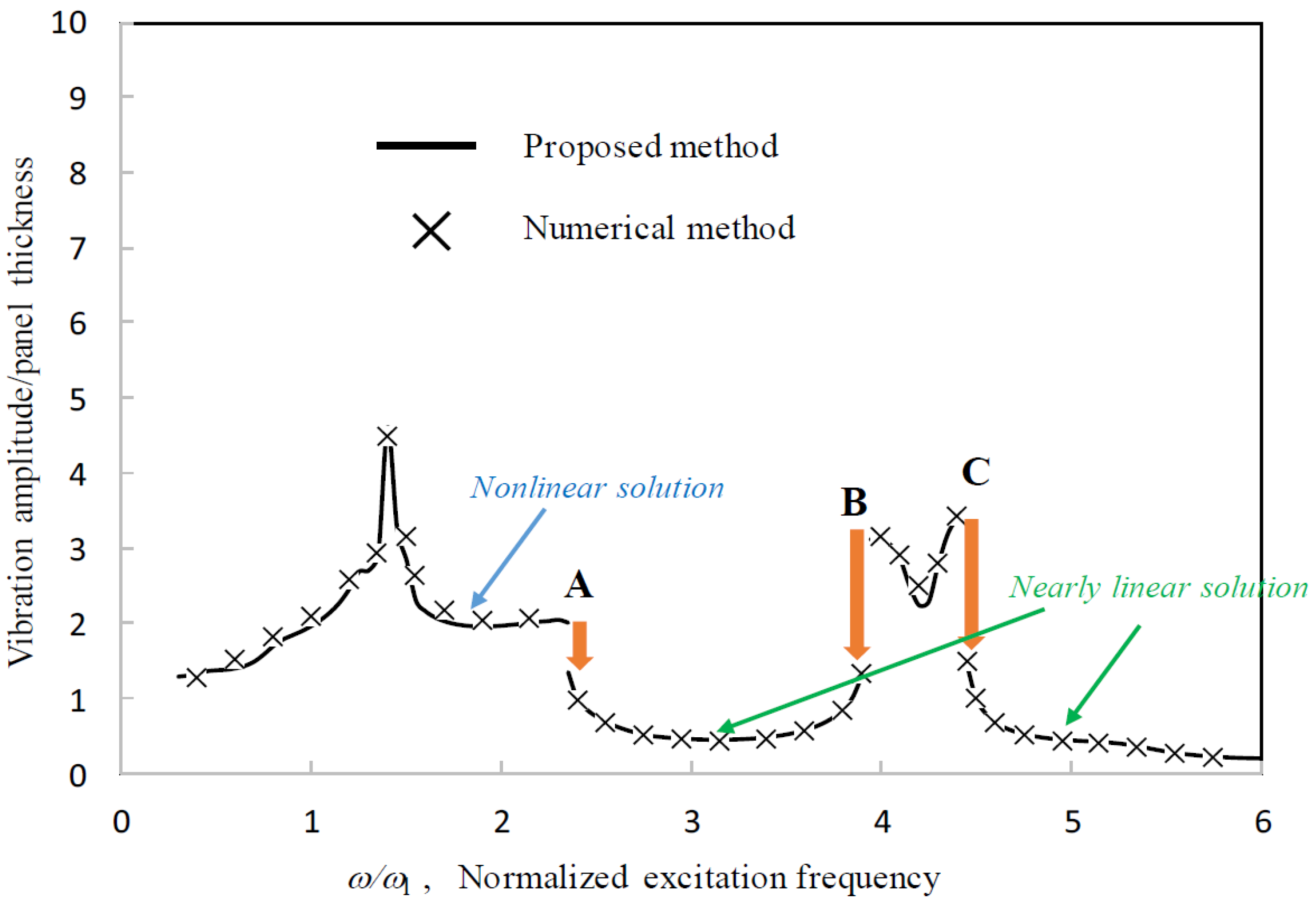
Figure 5, Figure 6 and 
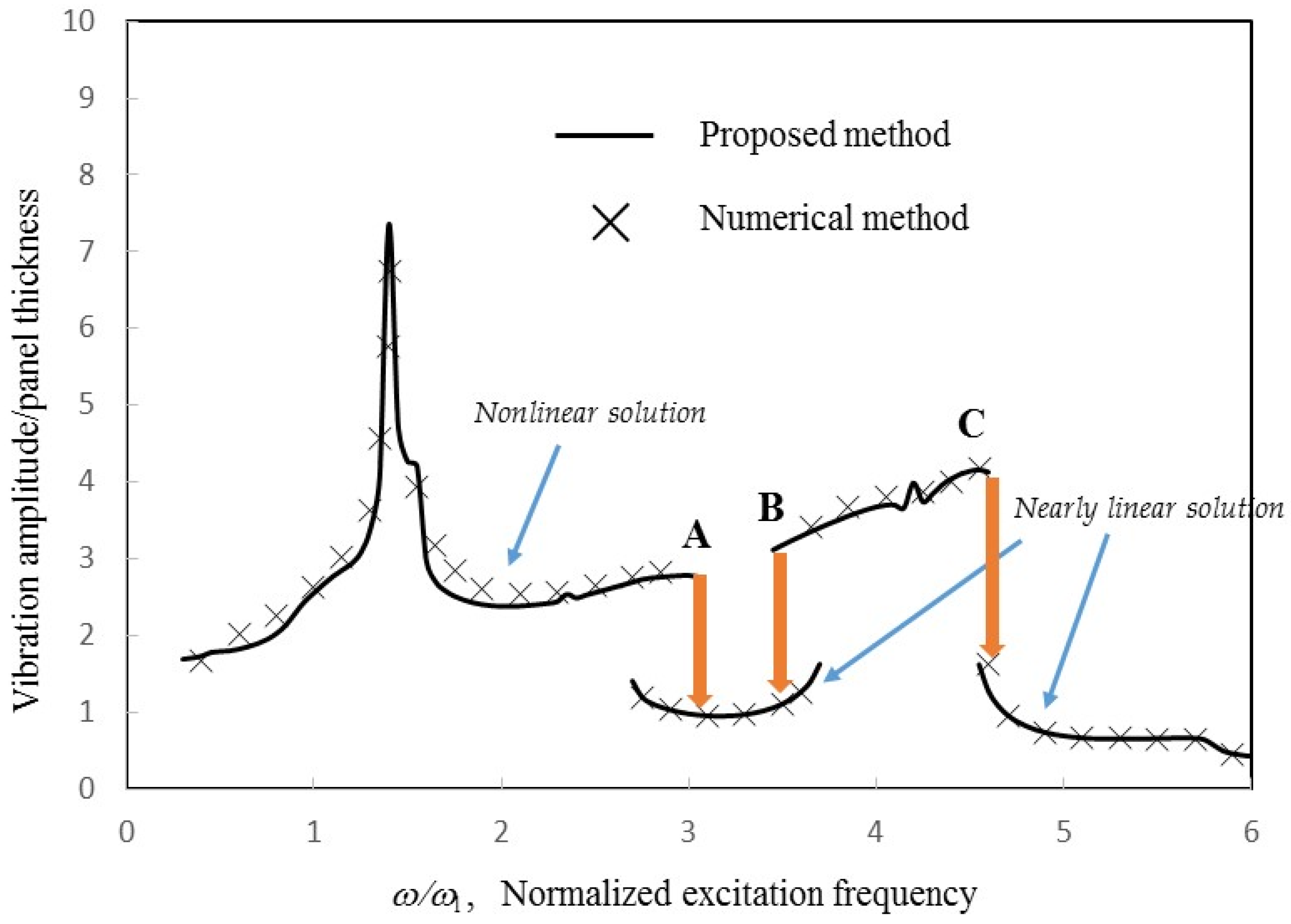
Figure 7 present the comparisons between the vibration amplitudes obtained from the present harmonic balance method and numerical method used in [6]. The results obtained from the two methods are generally in good agreement. Note that the numerical method is unable to generate the unstable solutions. For fair comparisons, the unstable solutions from the harmonic balance methods are not generated. In fact, the classical harmonic balance method can be coupled with the asymptotic numerical method, which enables the capture of unstable solutions (e.g., [21,22,23]). According to [14], the solutions from the proposed method come from the cubic algebraic equations transformed from the Duffing differential equations representing the nonlinear panel vibration. The unstable solutions occur when the cubic algebraic equations have three real solutions. Generally, the unstable solution is in between the nonlinear and nearly linear solutions. It is slightly lower than the real nonlinear solution around the peak frequency and slightly higher than the nearly linear solution when the excitation frequency is far from the peak frequency.
Relatively, the agreement in 
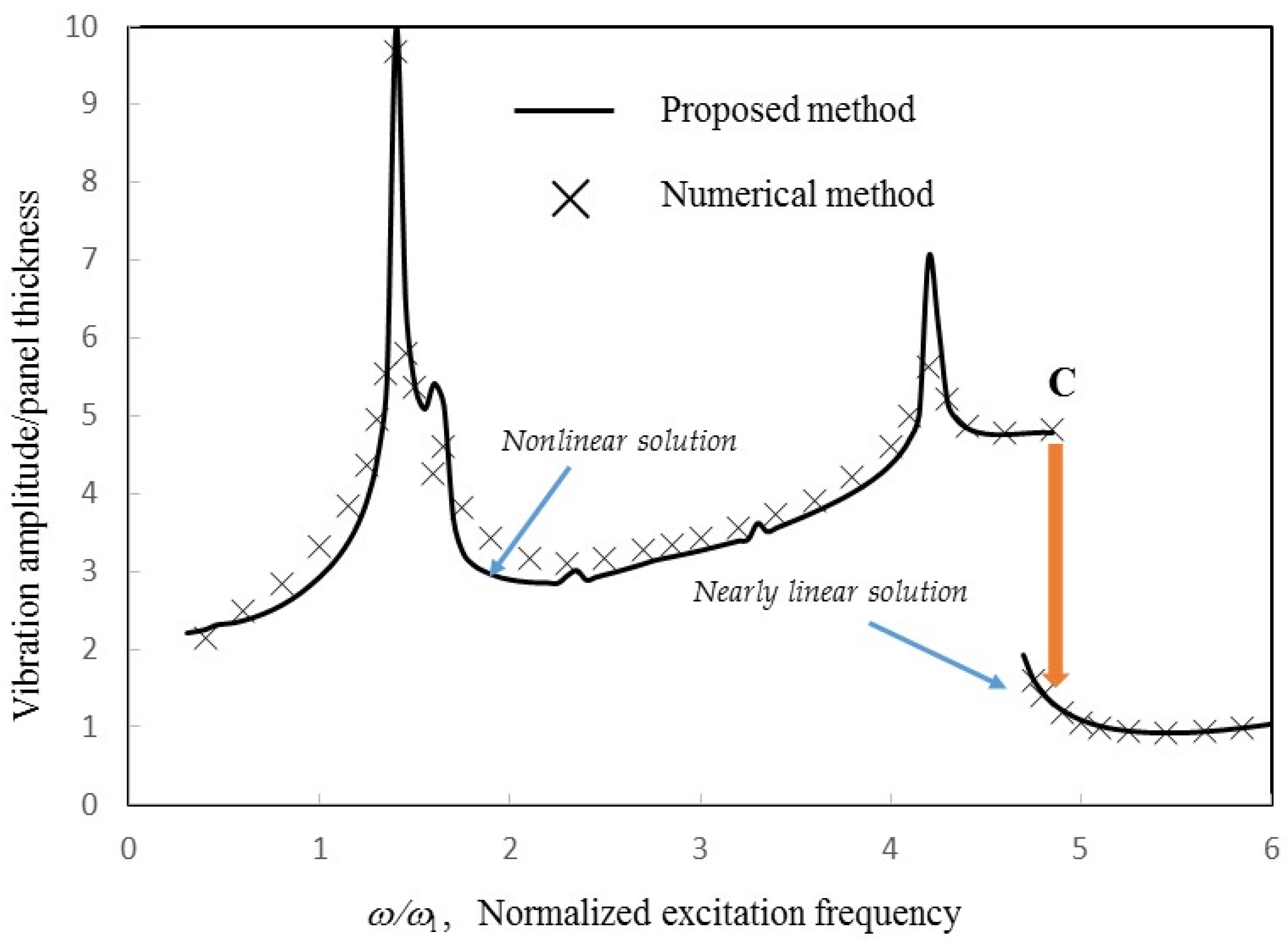
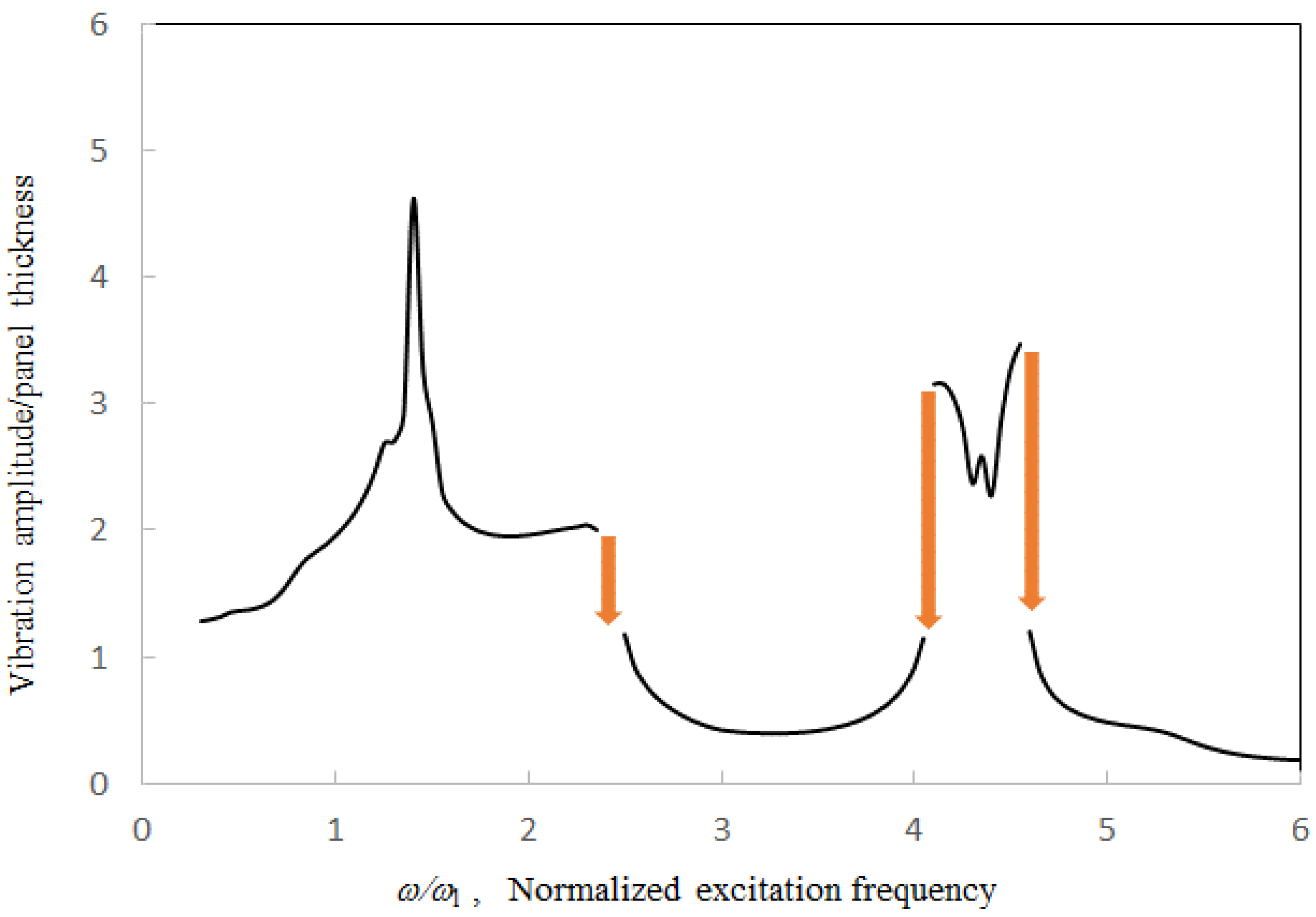
Figure 5 is the best because of smaller nonlinearity. In Figure 6 and 
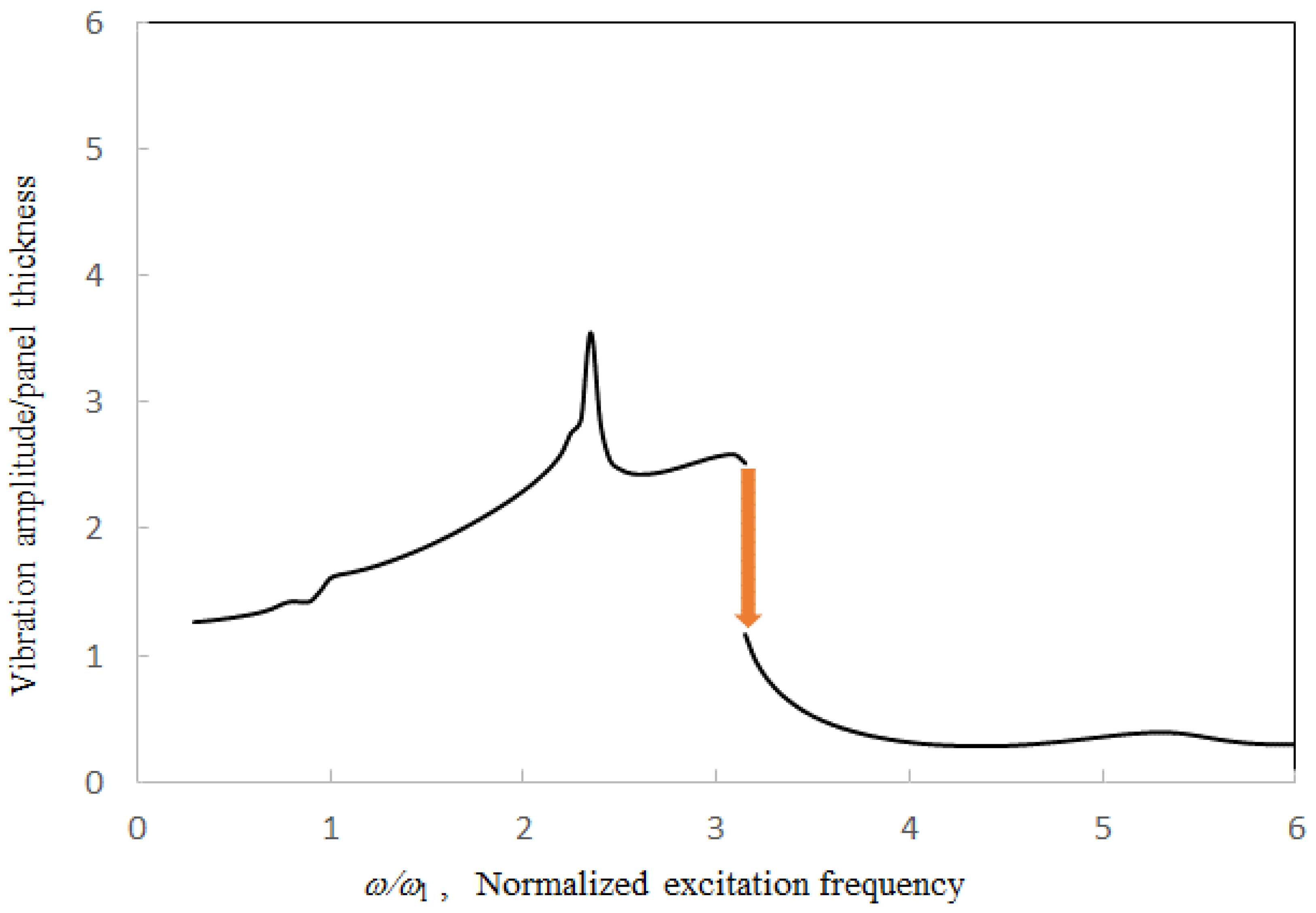
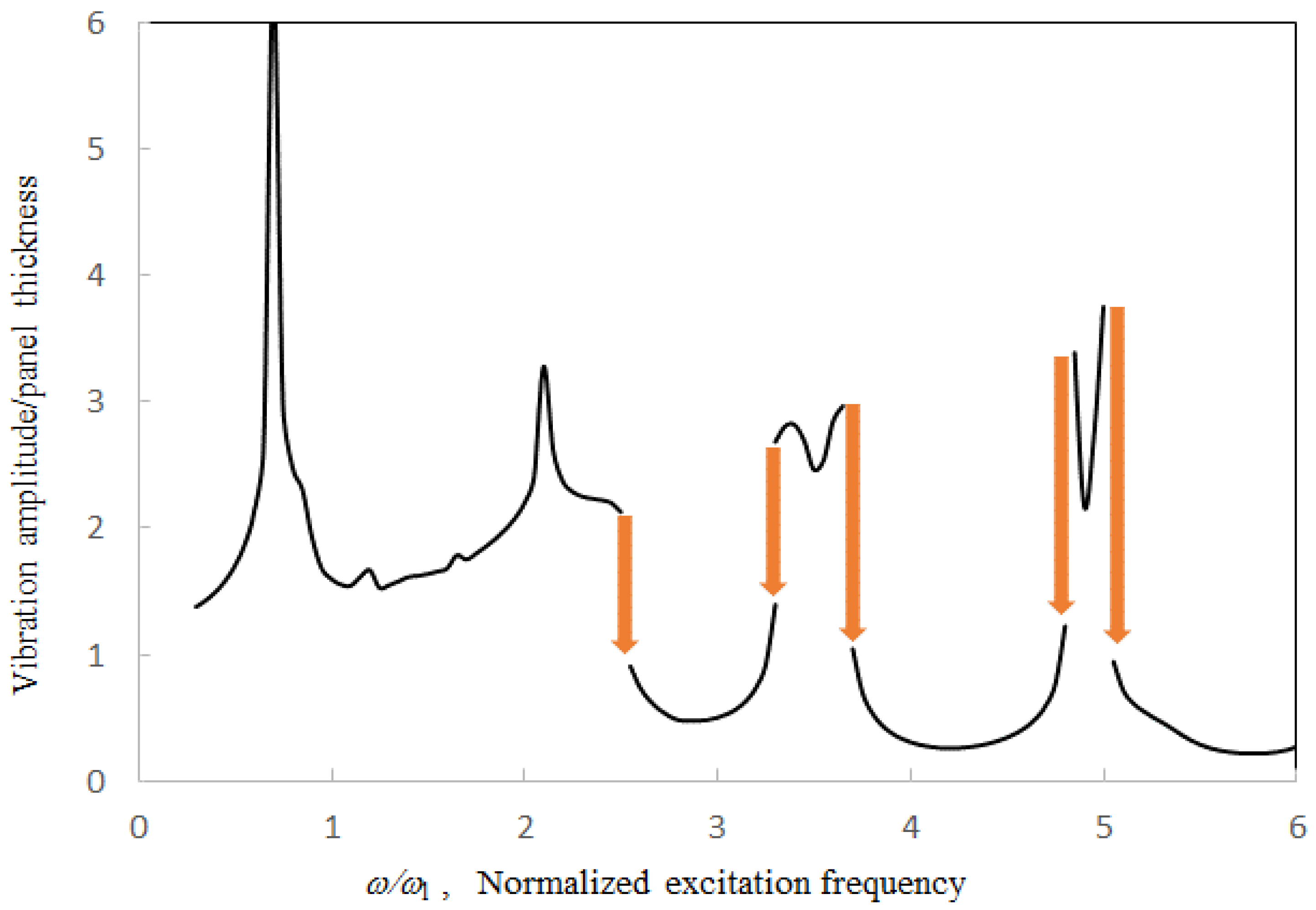
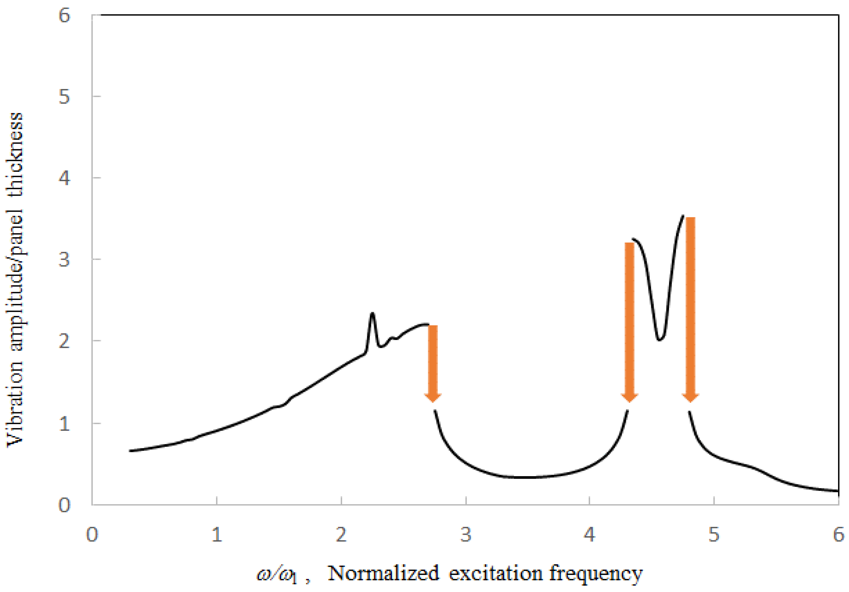
Figure 7, some deviations are observed around the major peak values. Note that there are some minor peaks around ω/ωl = 2.3 and 3.4 in Figure 7. In these three cases, the first acoustic resonances occur around ω/ω
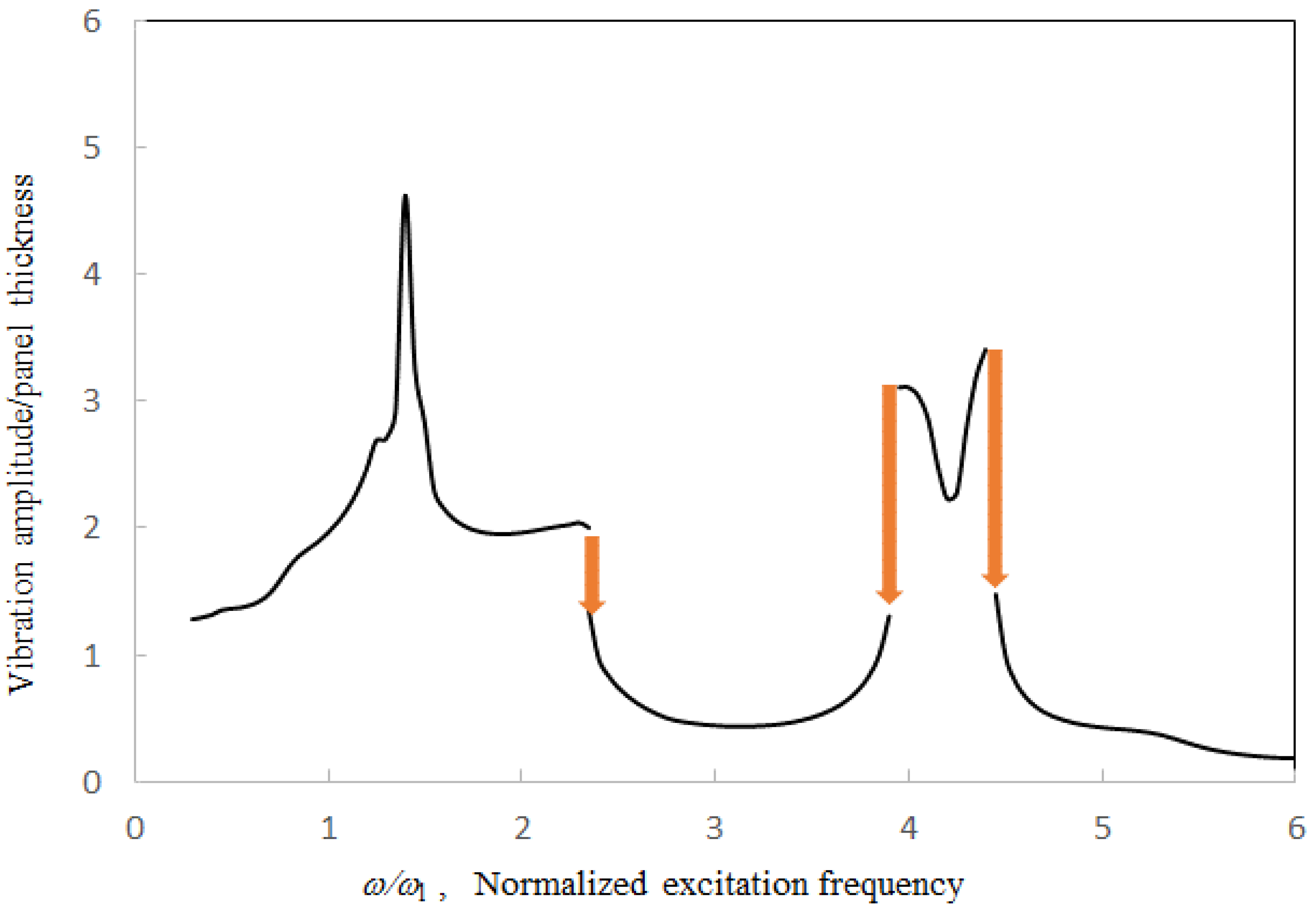
l = 1.4. In the case of γ = 2, the well-known jump phenomena, which are due to the first structural resonance and higher acoustic resonances, occurs around ω/ωl = 2.3, 3.9 and 4.5 (see Points A, B and C). The nonlinear solution line discontinues there. Generally, the nearly linear solution lines are much lower than the nonlinear solution lines. In the cases of γ = 4 and 8, the jump phenomena due to the first structural resonance and higher acoustic resonances occur at the higher frequencies. Unlike the trough on the solution line in the case of γ = 2, a small peak and a large peak occur on the nonlinear solution lines of γ = 4 and 8 around ω/ωl = 4.2, respectively. Besides, Points A and B in the case of γ = 4 are very close. There are no Points A and B in the case of γ = 8 (i.e., no discontinuous portion). In Figure 7, due to the large excitation level, the vibration responses are highly nonlinear. The nonlinear solution lines further extend so that Points A and B are joined and the linear solution line disappears. In this case, there is only one real solution obtained from the cubic algebraic equation transformed from the Duffing differential equations representing the nonlinear panel vibration. In the practical structural design of a similar structural–acoustic system, the disappearance of the linear solution (or small-amplitude solution), which is replaced by the nonlinear solution (or large-amplitude solution), implies that a stronger structural design is needed to overcome the larger vibration amplitude.
Figure 8, Figure 9 and Figure 10 show the vibration amplitude plotted against the excitation frequency for various tube lengths. The first peak value due to the acoustic resonance and first jump-down frequency increase with the tube length, while the first peak frequency and the first trough frequency decrease with the tube length. In the case of l = 10a, the tube length is the longest among the three cases. Thus, the second peak occurs around ω/ωl = 2.1, which is lower than the first jump-down frequency, and there are more acoustic resonant peaks on the solution line. In the case of l = 3a, the tube length is the shortest among the three cases. The trough occurs out of the frequency range (i.e. ω/ωl > 6).
Figure 11, Figure 12 and Figure 13 show the vibration amplitude plotted against the excitation frequency for various phase shift parameters. The first peak frequency due to the acoustic resonance, the first jump-down frequency, and the trough frequency increase with the phase shift parameter, while the first peak value decreases with the tube length. In the cases of θ = 5 and 10, it is implied that the tube boundaries are not perfectly rigid and the corresponding air particle velocities are non-zero. It is noted that the first peak is quite small, marginally detectable when the phase shift is only 8 degrees.
Moreover, the phase shift does not significantly affect the higher acoustic resonances. 
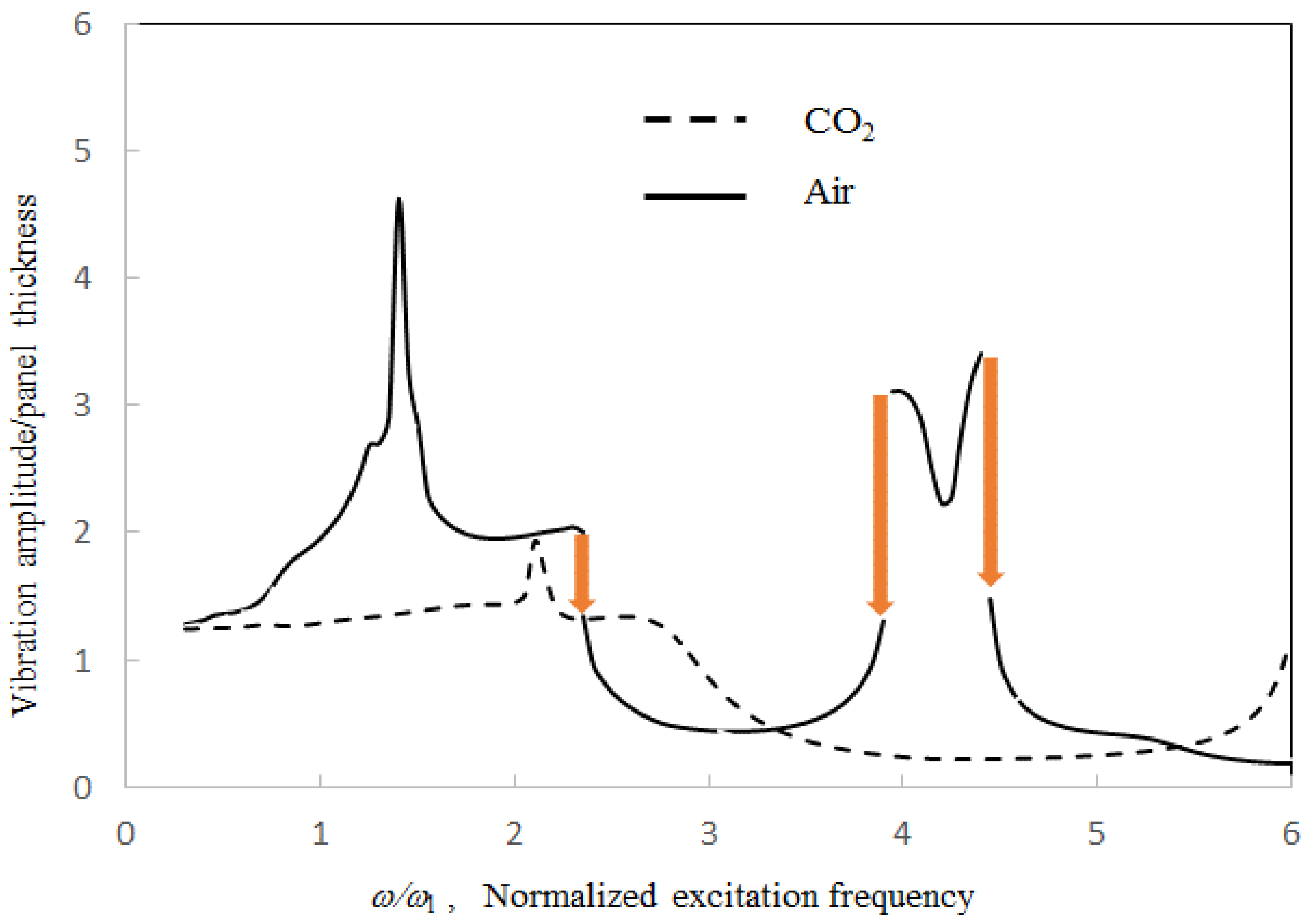
Figure 14 shows the vibration amplitudes of the tubes filled with air and CO2 plotted against the corresponding excitation frequency. The density of CO2 and the corresponding sound speed are about 50% higher than those in the case of air. There is a big difference between the two cases. In the case of CO2, the first peak is much smaller and the jump phenomenon disappears. The peaks due to higher acoustic resonances are out of the frequency range. In the practical structural design of a similar structural–acoustic system, the disappearance of the nonlinear solution (or large-amplitude solution), which is replaced by the linear solution (or small-amplitude solution), implies that a smaller amount of structural material is needed.

4. Conclusions

This paper has presented the analysis for the nonlinear vibration response of a rectangular tube with a flexible end and non-rigid acoustic boundaries. The structural–acoustic modal formulations have been developed from the partial differential equations, which represent the large-amplitude structural vibration of a flexible panel coupled with a cavity. The results obtained from the multi-level residue harmonic balance method and numerical method are generally in good agreement. The effects of excitation magnitude, tube length, and phase shift parameter, etc., are investigated. It can be concluded from the results that: (1) if the excitation level is very high, there is no linear solution at the medium frequency range, and a nonlinear solution occurs at that frequency range; (2) if the tube length is longer, more vibration peaks due to the acoustic resonances appear within the particular frequency range; (3) these peak values are also very sensitive to the phase shift parameter. As an example, the first peak is marginally detectable when the phase shift is only 8 degrees; (4) if the tube is filled with CO2, of which the density and corresponding sound speed are about 50% higher than those of air, the vibration peaks become very small or disappear within the particular frequency range.

Acknowledgments

The work described in this paper was fully supported by the CityU SRG [project No. 7004701].

Conflicts of Interest

The author declares no conflict of interest.

References

  1. Kinsler, L.E.; Frey, A.R.; Coppens, A.B.; Sanders, J.V. Fundamentals of Acoustics, 4th ed.; John Wiley & Sons Inc.: Hoboken, NJ, USA, 2000. [Google Scholar]
  2. Pretlove, A.J. Free vibrations of a rectangular panel backed by a closed rectangular cavity. J. Sound Vib. 1965, 2, 197–209. [Google Scholar] [CrossRef]
  3. Oldham, D.J.; Hillarby, S.N. The acoustical performance of small close fitting enclosures. Part I: Theoretical models. J. Sound Vib. 1991, 150, 261–281. [Google Scholar] [CrossRef]
  4. Lee, Y.Y.; Lee, E.W.M. Widening the sound absorption bandwidths of flexible micro-perforated curved absorbers using structural and acoustic resonances. Int. J. Mech. Sci. 2007, 49, 925–934. [Google Scholar] [CrossRef]
  5. Younesian, D.; Sadri, M.; Esmailzadeh, E. Primary and secondary resonance analyses of clamped-clamped micro-beams. Nonlinear Dyn. 2014, 76, 1867–1884. [Google Scholar] [CrossRef]
  6. Lee, Y.Y.; Su, R.K.L.; Ng, C.F.; Hui, C.K. The effect of the modal energy transfer on the sound radiation and vibration of a curved panel: Theory and experiment. J. Sound Vib. 2009, 324, 1003–1015. [Google Scholar] [CrossRef]
  7. Lee, Y.Y.; Poon, W.Y.; Ng, C.F. Anti-symmetric mode vibration of a curved beam subject to autoparametric excitation. J. Sound Vib. 2006, 290, 48–64. [Google Scholar] [CrossRef]
  8. Huang, J.L.; Su, R.K.L.; Lee, Y.Y.; Chen, S.H. Nonlinear vibration of a curved beam under uniform base harmonic excitation with quadratic and cubic nonlinearities. J. Sound Vib. 2011, 330, 5151–5164. [Google Scholar] [CrossRef]
  9. Kacem, N.; Hentz, S.; Pinto, D.; Reig, B.; Nguyen, V. Nonlinear dynamics of nanomechanical beam resonators: Improving the performance of NEMS-based sensors. Nanotechnology 2009, 20, 275501. [Google Scholar] [CrossRef] [PubMed]
  10. Kacem, N.; Hentz, S. Bifurcation topology tuning of a mixed behavior in nonlinear micromechanical resonators. Appl. Phys. Lett. 2009, 95, 183104. [Google Scholar] [CrossRef]
  11. Kacem, N.; Arcamone, J.; Perez-Murano, F.; Hentz, S. Dynamic range enhancement of nonlinear nanomechanical resonant cantilevers for highly sensitive NEMS gas/mass sensor applications. J. Micromech. Microeng. 2010, 20, 045023. [Google Scholar] [CrossRef]
  12. Kacem, N.; Baguet, S.; Duraffourg, L.; Jourdan, G.; Dufour, R.; Hentz, S. Overcoming limitations of nanomechanical resonators with simultaneous resonances. Appl. Phys. Lett. 2015, 107, 073105. [Google Scholar] [CrossRef] [Green Version]
  13. Leung, A.Y.T.; Guo, Z. Feed forward residue harmonic balance method for a quadratic nonlinear oscillator. Int. J. Bifurc. Chaos 2011, 21, 1783–1794. [Google Scholar] [CrossRef]
  14. Hasan, A.S.M.Z.; Lee, Y.Y.; Leung, A.Y.T. The multi-level residue harmonic balance solutions of multi-mode nonlinearly vibrating beams on an elastic foundation. J. Vib. Control 2016, 22, 3218–3235. [Google Scholar] [CrossRef]
  15. Lee, Y.Y.; Ng, C.F. Sound insertion loss of stiffened enclosure plates using the finite element method and the classical approach. J. Sound Vib. 1998, 217, 239–260. [Google Scholar] [CrossRef]
  16. Hui, C.K.; Lee, Y.Y.; Reddy, J.N. Approximate elliptical integral solution for the large amplitude free vibration of a rectangular single mode plate backed by a multi-acoustic mode cavity. Thin-Walled Struct. 2011, 49, 1191–1194. [Google Scholar] [CrossRef]
  17. Park, S.; Kim, H. Development of analytical impact force models for floor impact vibration and acoustic numerical analysis. Appl. Sci. 2016. [Google Scholar] [CrossRef]
  18. Luo, Z.; Zhu, Y.P.; Liu, H.P.; Wang, D.Y. Dynamic similitude design method of the distorted model on variable thickness cantilever plates. Appl. Sci. 2016. [Google Scholar] [CrossRef]
  19. Lee, Y.Y. The effect of leakage on the sound absorption of a nonlinear perforated panel backed by a cavity. Int. J. Mech. Sci. 2016, 107, 242–252. [Google Scholar] [CrossRef]
  20. Lee, Y.Y. Multi-level residue harmonic balance method for the transmission loss of a nonlinearly vibrating perforated panel. Int. J. Struct. Stab. Dyn. 2016, 16, 1450100. [Google Scholar] [CrossRef]
  21. Kacem, N.; Baguet, S.; Hentz, S.; Dufour, R. Computational and quasi-analytical models for non-linear vibrations of resonant MEMS and NEMS sensors. Int. J. Non-linear Mech. 2011, 46, 532–542. [Google Scholar] [CrossRef] [Green Version]
  22. Souayeh, S.; Kacem, N. Computational models for large amplitude nonlinear vibrations of electrostatically actuated carbon nanotube-based mass sensors. Sens. Actuators A 2014, 208, 10–20. [Google Scholar] [CrossRef]
  23. Jallouli, A.; Kacem, N.; Bourbon, G.; Le Moal, P.; Walter, V.; Lardies, J. Pull-in instability tuning in imperfect nonlinear circular microplates under electrostatic actuation. Phys. Lett. A 2016, 380, 3886–3890. [Google Scholar] [CrossRef]
Figure 1. The linear structural–acoustic model in [1].
Applsci 06 00424 g001
Figure 2. General concept of a structural–acoustic model.
Applsci 06 00424 g002
Figure 3. Schematic diagram of a rectangular tube with a flexible end and non-rigid acoustic boundaries.
Applsci 06 00424 g003
Figure 4. Acoustic mode shapes of the fully open and fully closed cavity boundaries.
Applsci 06 00424 g004
Figure 5. Comparison between the solutions obtained from the proposed method and numerical integration method [6] (number of structural modes = 2, number of acoustic modes = 4, l = 5a, γ = 2, θ = 0; the orange arrows represent the “jump phenomenon”; “A”, “B”, and “C” represent the particular points on the solution curve).
Applsci 06 00424 g005
Figure 6. Comparison between the solutions obtained from the proposed method and numerical integration method [6] (number of structural modes = 2, number of acoustic modes = 4, l = 5a, γ = 4, θ = 0; the orange arrows represent the “jump phenomenon”; “A”, “B”, and “C” represent the particular points on the solution curve).
Applsci 06 00424 g006
Figure 7. Comparison between the solutions obtained from the proposed method and numerical integration method [6] (number of structural modes = 2, number of acoustic modes = 4, l = 5a, γ = 8, θ = 0; the orange arrow represents the “jump phenomenon”; “C” represents the particular point on the solution curve).
Applsci 06 00424 g007
Figure 8. Vibration amplitude ratio versus normalized excitation frequency for various duct lengths (number of structural modes = 2, number of acoustic modes = 4, γ = 2, θ = 0, l = 3a; the orange arrow represents the “jump phenomenon”).
Applsci 06 00424 g008
Figure 9. Vibration amplitude ratio versus normalized excitation frequency for various duct lengths (number of structural modes = 2, number of acoustic modes = 4, γ = 2, θ = 0, l = 5a; the orange arrows represent the “jump phenomenon”).
Applsci 06 00424 g009
Figure 10. Vibration amplitude ratio versus normalized excitation frequency for various duct lengths (number of structural modes = 2, number of acoustic modes = 4, γ = 2, θ = 0, l = 10a; the orange arrows represent the “jump phenomenon”).
Applsci 06 00424 g010
Figure 11. Vibration amplitude ratio versus normalized excitation frequency for various acoustic boundary conditions (number of structural modes = 2, number of acoustic modes = 4, γ = 2, θ = 0, l = 5a; the orange arrows represent the “jump phenomenon”).
Applsci 06 00424 g011
Figure 12. Vibration amplitude ratio versus normalized excitation frequency for various acoustic boundary conditions (number of structural modes = 2, number of acoustic modes = 4, γ = 2, θ = 5, l = 5a; the orange arrows represent the “jump phenomenon”).
Applsci 06 00424 g012
Figure 13. Vibration amplitude ratio versus normalized excitation frequency for various acoustic boundary conditions (number of structural modes = 2, number of acoustic modes = 4, γ = 2, θ = 8, l = 5a; the orange arrows represent the “jump phenomenon”).
Applsci 06 00424 g013
Figure 14. Vibration amplitude ratio versus normalized excitation frequency for the cases of air and CO2 (number of structural modes = 2, number of acoustic modes = 4, l = 5a, γ = 2, θ = 0; the orange arrows represent the “jump phenomenon”).
Applsci 06 00424 g014
Table 1. Numbers of equations for the cubic nonlinear undamped beam problem.
Solution MethodZero Level (1 Harmonic Term)1st Level (2 Harmonic Terms)2nd Level (3 Harmonic Terms)
No. of nonlinear algebraic equationsNo. of linear algebraic equationsNo. of nonlinear algebraic equationsNo. of linear algebraic equationsNo. of nonlinear algebraic equationsNo. of linear algebraic equations
Proposed harmonic balance method101213
Classical harmonic balance method102030
Table 2. Acoustic mode convergence study (1st level solution, number of structural modes = 2, l = 5a, γ = 4).
ω/ωcNo. of Acoustic Modes
149
1.899.83100.00100 1
2.899.0999.97100 1
4.899.97100.24100 1
1 The amplitudes are normalized as 100.
Table 3. Structural mode convergence study (1st level solution, number of acoustic modes = 4, l = 5a, γ = 4).
ω/ωcNo. of Structural Modes
123
1.899.20100.00100 1
2.898.77100.00100 1
4.870.2899.97100 1
1 The amplitudes are normalized as 100.
Table 4. Harmonic term convergence study (number of structural modes = 2, number of acoustic modes = 4, l = 5a, γ = 4).
ω/ωcNo. of Harmonic Terms
1 (Zero Level)2 (1st Level)3 (2nd Level)
1.8103.60100.66100 1
2.8100.17100.00100 1
4.899.83100.00100 1
1 The amplitudes are normalized as 100.

