A Calibration Method for Nonlinear Mismatches in M-Channel Time-Interleaved Analog-to-Digital Converters Based on Hadamard Sequences

Abstract

The time-interleaved analog-to-digital converter (TIADC) is an architecture used to achieve a high sampling rate and high dynamic performance. However, estimation and compensation methods are required to maintain the dynamic performance of the constituent analog-to-digital converters (ADCs) due to channel mismatches. This paper proposes a blind adaptive method to calibrate the nonlinear mismatches in M-channel TIADCs (M-TIADCs). The nonlinearity-induced error signal is reconstructed by the proposed multiplier Hadamard transform (MHT) structure, and the nonlinear parameters are estimated by the filtered-X least-mean square (FxLMS) algorithm. The performance of cascade calibration is also analyzed. The numerical simulation results show that the proposed method consumes much less hardware resources while maintaining the calibration performance.

1. Introduction

The time-interleaved analog-to-digital converter (TIADC) is proposed to meet the fast increasing demand for a high sampling rate in modern mixed-signal processing systems, e.g., radar, communication and measurement equipment. The sampling rate of an M-channel TIADC (M-TIADC) is M-times the sampling rate of the sub-ADCs, and the resolution of the M-TIADC is the same as the resolution of sub-ADCs in the ideal case. However, due to non-ideal circuit implementations, spurious components arise because of the discrepancies among the sub-ADCs, distorting the sampled signal and degrading the effective resolution of the sub-ADCs. Therefore, calibration (compensation) methods are required to suppress the spurious components and restore the dynamic performance of sub-ADCs.

A large number of papers devoted to estimation and compensation methods for TIADCs has been published during the past few decades. Most of them aim at the compensation methods for the linear mismatches, including gain, time-skew and frequency response mismatches [1,2,3,4,5,6,7,8,9,10,11,12,13,14,15,16,17,18,19,20]. By comparison, relatively few papers have been published to address the nonlinear mismatches problem, which stems from the imperfection of front-end circuits, as well as the differential and integral nonlinearities of sub-ADCs [21,22,23,24,25,26,27,28].

A study of differential nonlinearities (DNL) and integral nonlinearities (INL) in M-TIADC is presented in [22]. It is pointed out that the DNL and INL of a TIADC are smaller than the DNL and INL errors for individual sub-ADCs. The channel linearity mismatch effects in TIADCs are analyzed and simulated in [21], in which several distinct features of nonlinear mismatch are shown. A nonlinear hybrid filter banks model of TIADCs is proposed in [29], where the input-output relationship of TIADCs with nonlinear mismatches is formulated. Several methods are proposed following the analysis and model mentioned above. A method exploiting the inverse function of the INL of each sub-ADC is proposed in [30] to compensate for the INL mismatches in M-TIADCs. However, the inverse function can only be measured by interrupting the normal sampling operation. A randomization-based calibration method is presented in [31] with the cost of additional converters, which is also the main drawback of the methods exploiting reference channels [24]. A digital compensation method that relies on the foreground estimated nonlinearities is presented in [26], where a sinusoidal signal is employed as the training signal during the estimation procedure. A blind calibration method is proposed in [27,28] for 2-TIADCs and extended in [25] for M-TIADCs.

The bandwidth efficient (BWE) method proposed in [25] is able to calibrate the nonlinear mismatches in M-TIADCs, as long as the mismatch-induced error signals are present in the input-free band, which is generated by a slight oversampling. However, there are two major drawbacks of the BWE method. Firstly, it is not only resource consuming, but also cumbersome to generate the sinusoidal modulation sequences needed in the BWE method. Secondly, two sets of variable multipliers are exploited for modulation and for weighting, respectively, which means a large number of multipliers is required. These two drawbacks are overcome by the method proposed in this paper.

In this paper, a blind calibration method exploiting the binary Hadamard sequences is proposed for nonlinear mismatches in M-TIADCs ($M=1,2,4,8,\dots$). Our method consumes much less hardware resources while maintaining the bandwidth efficiency and calibration performance of the BWE method. The sinusoidal modulation sequences in the BWE method are replaced by the binary Hadamard sequences in our approach, which brings the following two benefits. Firstly, the Hadamard sequences are much easier to generate compared with the sinusoidal sequences because there are only 1 and −1 in the binary Hadamard sequences. Thus, the resource-consuming and complicated circuits used to generate sinusoidal modulation sequences are saved. Secondly, the multipliers for modulation are no longer necessary because multiplying by 1 and −1 can be accomplished by just changing the sign of the modulated signal, which means that the number of multipliers is reduced by nearly half. The price is that our method can only deal with the nonlinear mismatch problem in TIADCs where the number of channels M is the power of two, i.e., $M=1,2,4,8,\dots$, while the BWE method is able to calibrate TIADCs with any integer number of channels. Nevertheless, this drawback has limited restriction on the application of our method because the number of channels M is the power of two in most practical TIADC systems.

Although Hadamard sequences (Hadamard transforms) are also exploited to deal with the frequency response problem in M-TIADCs [32], there are fundamental differences between these two papers. Firstly, the focus of this paper is the nonlinear mismatch problem, while the focus of [32] is the frequency response mismatch problem; secondly, the method proposed in this paper is totally blind, while the method adopted in [32] requires a training sequence.

The rest of this paper is organized as follows. In Section 2, the nonlinear mismatch-induced error is analyzed, and a model exploiting the binary Hadamard sequences is proposed. A calibration structure is presented in Section 3 to calibrate the mismatch error based on the model shown in Section 2. The numerical simulation results are presented in Section 4 to demonstrate the performance of our method and the superiorities over existing methods. The concluding remarks are presented in Section 5.

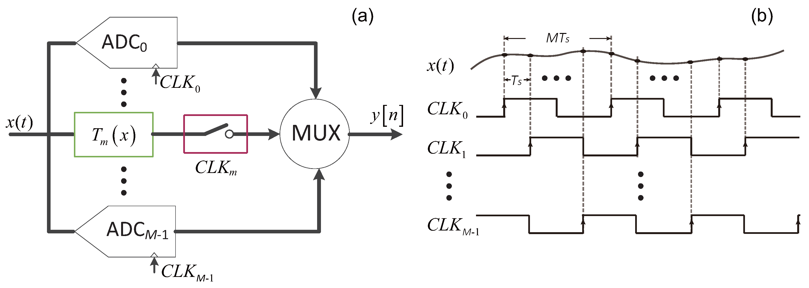
2. Nonlinear Mismatches in M-TIADC

Figure 1 illustrates a TIADC consisting of M sub-ADCs and the timing diagram of the sampling clocks for the constituent ADCs. The periods of all of these clocks are $M{T}_s$; thus, the overall sampling period of the TIADC is $T_s$. The nonlinear characteristics of the m-th sub-ADC, i.e., ADC${}_m$, are represented by the polynomial $T_m\left(x\right)=x+{\sum }_{l=2}^L{\mathsf{\alpha }}_{m,l}{x}^l$, where x is the band-limited analog input signal $x\left(t\right)$ with bandwidth ${\mathsf{\Omega }}_c<2\mathsf{\pi }/T_s$, and ${\mathsf{\alpha }}_{m,l},l=2,\dots ,L$ are the polynomial coefficients representing the nonlinearity of channel m. As the focus of this paper is the compensation method for the nonlinear behavior of TIADCs, we assume that the linear frequency response mismatches have been calibrated. The quantization process is not considered throughout the theoretical analysis, because its effect can be modeled as adding white noise. Only static (frequency independent) nonlinearities are considered in this paper since static nonlinearities are the dominating part of nonlinear feature in most applications. The nonlinearities are modeled as polynomials with different parameters. This model cannot describe all nonlinearities in ADCs; however, it is sufficient to model several important nonlinearities, such as saturation and dead zone nonlinearities.

The time-domain output of M-TIADC with nonlinear mismatches is:

$$y\left[n\right]=x\left[n\right]+\sum _{l=2}^L{\mathsf{\alpha }}_{n,l}{x}^l\left[n\right],$$

(1)

where ${\mathsf{\alpha }}_{n,l}={\mathsf{\alpha }}_{n+M,l}$ and $x\left[n\right]=x\left(n{T}_s\right)$ is the ideally sampled input signal.

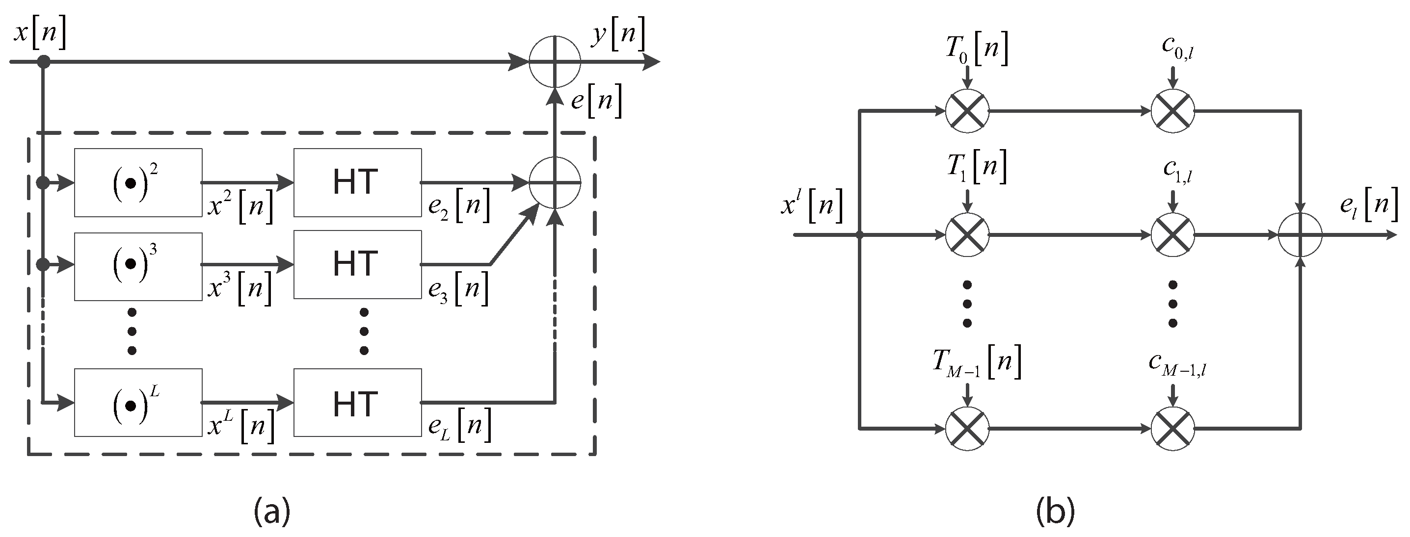
2.1. Mismatch-Induced Error Signal

By finding the discrete-time Fourier transform (DTFT) of $y\left[n\right]$, the output in the frequency domain is written as [25]:

$$Y(e^{j\mathsf{\omega }})=X(e^{j\mathsf{\omega }})+E(e^{j\mathsf{\omega }}),$$

(2)

where:

$$E(e^{j\mathsf{\omega }})=\sum _{k=0}^{M-1}{E}_k(e^{j\mathsf{\omega }})$$

(3)

with:

$$E_k(e^{j\mathsf{\omega }})=\sum _{l=2}^L\frac{1}{{\left(2\mathsf{\pi }\right)}^{l-1}}{A}_l\left(k\right)X^{*l}\left(e^{j(\mathsf{\omega }-\frac{2\mathsf{\pi }}{M}k)}\right)$$

(4)

and:

$$A_l\left(k\right)=\frac{1}{M}{\mathsf{\alpha }}_{m,l}{e}^{-j\frac{2\mathsf{\pi }}{M}mk},$$

(5)

in which $X^{*l}(e^{j\mathsf{\omega }})$ represents the l-fold convolution of $X(e^{j\mathsf{\omega }})$.

The error signal $E(e^{j\mathsf{\omega }})$ can be expressed in matrix form as:

$$E(e^{j\mathsf{\omega }})=\sum _{l=2}^L{\breve{E}}_l=\sum _{l=2}^L{\overrightarrow{X^l}}^T\mathit{W}{\overrightarrow{\mathsf{\alpha }}}_l$$

(6)

with:

$$\overrightarrow{X^l}=\frac{1}{{\left(2\mathsf{\pi }\right)}^{l-1}}{\left[X^{*l}(e^{j\mathsf{\omega }})X^{*l}(e^{j(\mathsf{\omega }-\frac{2\mathsf{\pi }}{M})})\cdots X^{*l}(e^{j(\mathsf{\omega }-\frac{2(M-1)\mathsf{\pi }}{M})})\right]}^T,$$

(7)

$$\mathit{W}=\left[\begin{array}{cccc}1& 1& \cdots & 1\\ 1& e^{-j\frac{2\mathsf{\pi }}{M}}& \cdots & e^{-j\frac{2(M-1)\mathsf{\pi }}{M}}\\ ⋮& ⋮& \ddots & ⋮\\ 1& e^{-j\frac{2(M-1)\mathsf{\pi }}{M}}& \cdots & e^{-j\frac{2(M-1)(M-1)\mathsf{\pi }}{M}}\end{array}\right]$$

(8)

being the discrete Fourier transform (DFT) matrix and:

$${\overrightarrow{\mathsf{\alpha }}}_l={[{\mathsf{\alpha }}_{0,l}{\mathsf{\alpha }}_{1,l}\cdots {\mathsf{\alpha }}_{M-1,l}]}^T$$

(9)

being the nonlinear coefficients vectors.

In the next subsection, the error signal $E(e^{j\mathsf{\omega }})$ is represented by the binary Hadamard matrix of order M, and a model for M-TIADC exploiting the multiplier Hadamard transform (MHT) structure is presented.

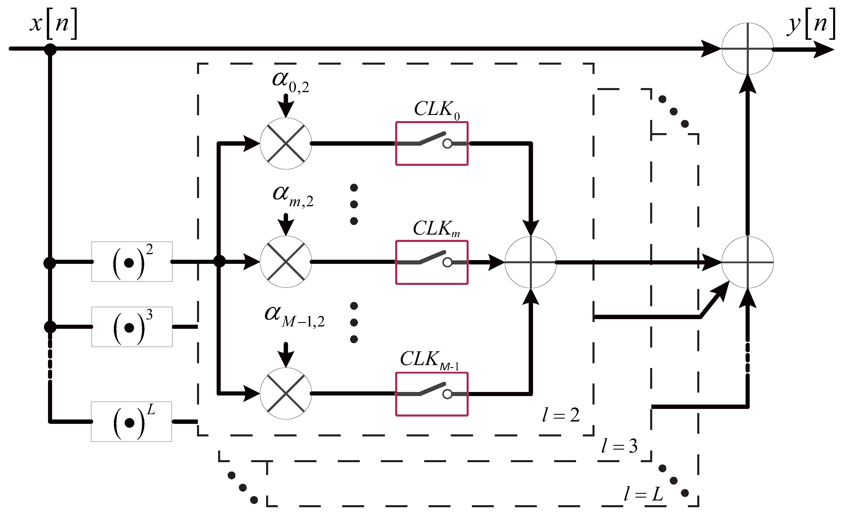
2.2. Model of M-TIADC Exploiting Hadamard Sequences

The error signal $E(e^{j\mathsf{\omega }})$ can be interpreted as the sum of $L-1$ gain-mismatched M-TIADC output, i.e., each ${\breve{E}}_l$ corresponding to the output of an M-TIADC with gain ${\mathsf{\alpha }}_{0,l},{\mathsf{\alpha }}_{1,l},\cdots ,{\mathsf{\alpha }}_{M-1,l}$ for the constituent channels where the input signal is $\frac{1}{{\left(2\mathsf{\pi }\right)}^{l-1}}{X}^{*l}(e^{j\mathsf{\omega }})$, i.e., $x^l\left[n\right]$ in the time domain. This interpretation is illustrated in Figure 2.

The Hadamard transform is exploited to model M-TIADCs with gain and timing-skew mismatches in [8]. As the nonlinear mismatches are interpreted as a group of TIADCs with gain mismatches in this paper, we utilize the Hadamard transform to model M-TIADCs with nonlinear mismatches, as well. The binary Hadamard matrix ${\mathit{F}}_M$ of order M exploited in this paper is defined by:

$${\mathit{F}}_2=\left[\begin{array}{cc}1& 1\\ 1& -1\end{array}\right]$$

(10)

and:

$${\mathit{F}}_{2m}=\left[\begin{array}{cc}{F}_m& F_m\\ F_m& -F_m\end{array}\right].$$

(11)

Exploiting the binary Hadamard matrix ${\mathit{F}}_M$, the error signal $E(e^{j\mathsf{\omega }})$ is rewritten as:

$$E(e^{j\mathsf{\omega }})=\sum _{l=2}^L\frac{1}{{\left(2\mathsf{\pi }\right)}^{l-1}}{\overrightarrow{X^l}}^T\mathit{U}{\overrightarrow{c}}_l,$$

(12)

where:

$${\overrightarrow{c}}_l=\frac{1}{M}{\mathit{F}}_M{\overrightarrow{\mathsf{\alpha }}}_l$$

(13)

representing the nonlinearities’ related coefficients and:

$$\mathit{U}=\frac{1}{M}\mathit{W}{\mathit{F}}_M$$

(14)

denoting the discrete Fourier transform of ${\mathit{F}}_M$. Two properties of the binary Hadamard matrix ${\mathit{F}}_M$ are exploited in the above derivations, which are ${\mathit{F}}_M{\mathit{F}}_M^T=M\mathit{I}$ and ${\mathit{F}}_M={\mathit{F}}_M^T$, where $\mathit{I}$ is the identity matrix and ${(•)}^T$ denotes the transpose of $(•)$.

By calculating the inverse discrete-time Fourier transform (IDTFT) of $E(e^{j\mathsf{\omega }})$, the error signal in the time-domain is expressed as:

$$e\left[n\right]=\sum _{l=2}^L{x}^l\left[n\right]\sum _{k=0}^{M-1}{T}_k\left[n\right]c_{k,l},$$

(15)

where $T_k\left[n\right]$ is the k-th binary Hadamard sequence of length M, which is also the k-th row (or column) of the binary Hadamard matrix ${\mathit{F}}_M$. Utilizing the time-domain expression of error signal $e\left[n\right]$, a model based on the binary Hadamard sequences is presented in Figure 3. Although multipliers are still used to represent the modulation by the Hadamard sequences $T_k\left[n\right]$ in Figure 3, they do not necessarily exist in the hardware implementation because modulation by the binary Hadamard sequences can be implemented by just changing the sign of the modulated signal $x^l\left[n\right]$.

The model shown in Figure 3, which is termed the multiplier Hadamard transform (MHT) structure in this paper, reveals that the nonlinearity-induced error signal $e\left[n\right]$ can be regarded as the sum of the weighted Hadamard transform of the power terms $x^l\left[n\right],l=2,\dots ,L$. In order to calibrate the nonlinearity and nonlinear mismatches, a calibration structure is proposed in the next section based on the presented signal model based on the binary Hadamard sequences.

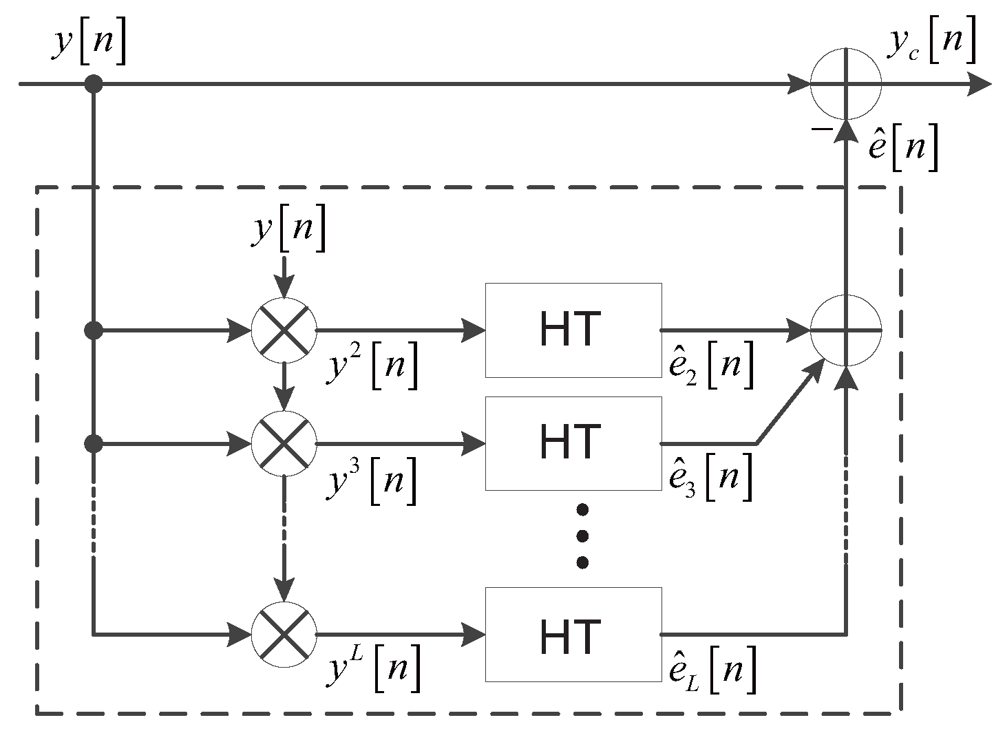
3. Adaptive Background Calibration Method

Based on the model presented in Figure 3, an adaptive blind calibration method for nonlinear mismatch error in M-TIADCs is proposed in this section. Our method can track the small variation of the nonlinear parameters, and no prior information about the input signal is required. The only requirement is a slight oversampling, which is anyhow commonly adopted in most practical TIADC systems. Compared with the approach proposed in [25], our method consumes much less hardware resources by replacing the sinusoidal modulation sequences with the binary Hadamard sequences.

The basic principle of our calibration method is to reconstruct the error signal $e\left[n\right]$ exploiting the estimated nonlinear parameters ${\widehat{c}}_{k,l}\left[n\right]$ and then subtract it from the M-TIADC output $y\left[n\right]$. The nonlinearities’ induced error signal in the input-free band stemming from oversampling is filtered out to estimate the nonlinear parameters utilizing the filtered-X least mean square (FxLMS) algorithm.

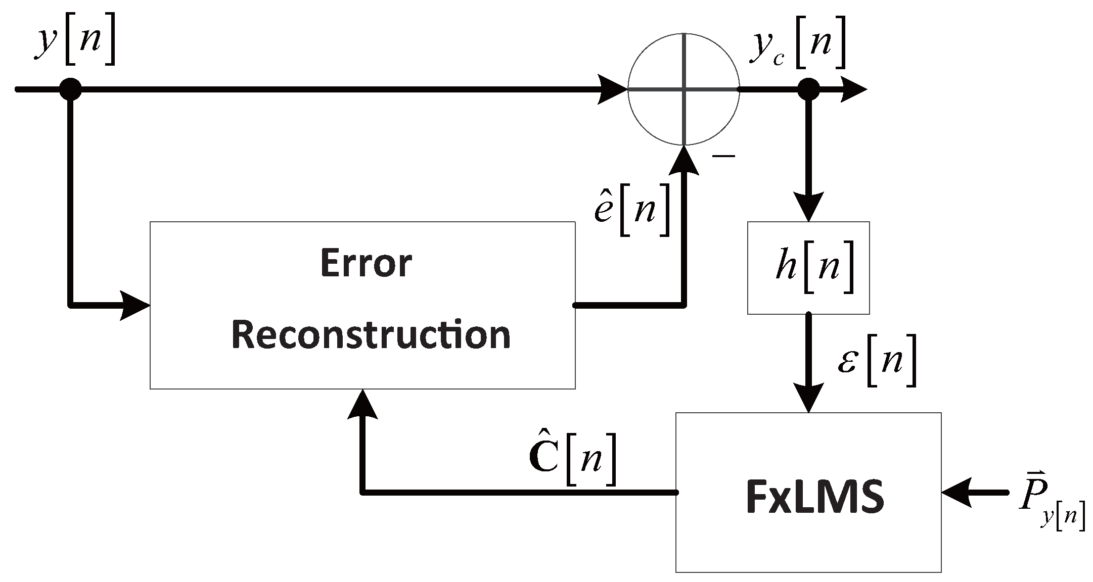
3.1. Calibration Structure

The error signal $e\left[n\right]$ can be ideally reconstructed exploiting the MHT structure if the input $x\left[n\right]$ is available and the nonlinear coefficients are precisely estimated. However, we cannot achieve perfect reconstruction even if the nonlinear parameters are known because only the M-TIADC output $y\left[n\right]$ is available. One solution is approximating $x\left[n\right]$ by $y\left[n\right]$. This is reasonable in a well-designed TIADC, which is a weakly nonlinear system, because the energy of error signal $e\left[n\right]$ is much smaller than the energy of the input signal. Thus, the reconstructed error signal is expressed as:

$$\widehat{e}\left[n\right]=\sum _{l=2}^L{y}^l\left[n\right]\sum _{k=0}^{M-1}{T}_k\left[n\right]{\widehat{c}}_{k,l}\left[n\right].$$

(16)

By subtracting the reconstructed error $\widehat{e}\left[n\right]$ from the M-TIADC output $y\left[n\right]$, the calibrated TIADC output signal is written as:

$$y_c\left[n\right]=x\left[n\right]+{\overrightarrow{T}}_n^T(\mathit{C}-\widehat{\mathit{C}}\left[n\right]){\overrightarrow{P}}_{y\left[n\right]}+{\overrightarrow{T}}_n^T\mathit{C}{\overrightarrow{R}}_{e\left[n\right]},$$

(17)

where ${\overrightarrow{T}}_n={[T_0\left[n\right]T_1\left[n\right]\cdots T_{M-1}\left[n\right]]}^T$, $\mathit{C}=[{\overrightarrow{c}}_2{\overrightarrow{c}}_3\cdots {\overrightarrow{c}}_L]$, ${\overrightarrow{R}}_{e\left[n\right]}={\overrightarrow{P}}_{x\left[n\right]}-{\overrightarrow{P}}_{y\left[n\right]}$ and $\widehat{\mathit{C}}\left[n\right]$ is the estimated version of $\mathit{C}$. As the power of ${\overrightarrow{R}}_{e\left[n\right]}$ is far less than the power of ${\overrightarrow{P}}_{x\left[n\right]}$ in a weakly nonlinear system, the power of the residual error signal $e_r\left[n\right]={\overrightarrow{T}}_n^T\mathit{C}\left[n\right]{\overrightarrow{R}}_{e\left[n\right]}$ is far less than the power of error $e\left[n\right]$ when the estimated coefficients $\widehat{\mathit{C}}\left[n\right]$ converge to the true nonlinear parameters $\mathit{C}$. More specifically, the magnitude of the error signal is suppressed from the order of $O\left(c_{k,l}\right)$ to the order of $O({(c_{k,l})}^2)$ exploiting the MHT calibration structure. Thus, the power of the error signal decreases from the order of $O({(c_{k,l})}^2)$ to the order of $O({(c_{k,l})}^4)$.

The calibration structure is shown in Figure 4. The reconstructed error signal $\widehat{e}\left[n\right]$ is generated utilizing the MHT schemes with input $y\left[n\right]$.

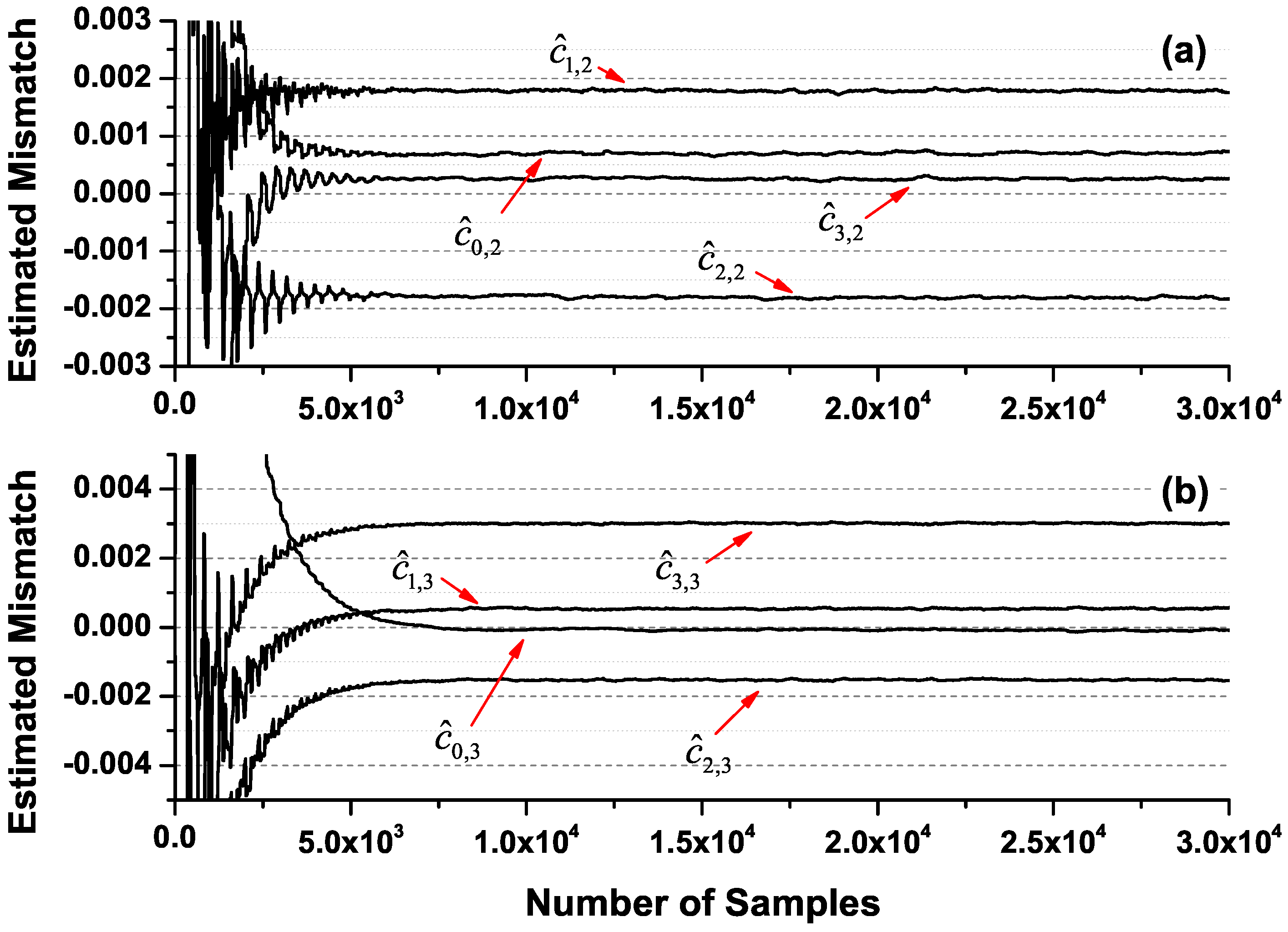
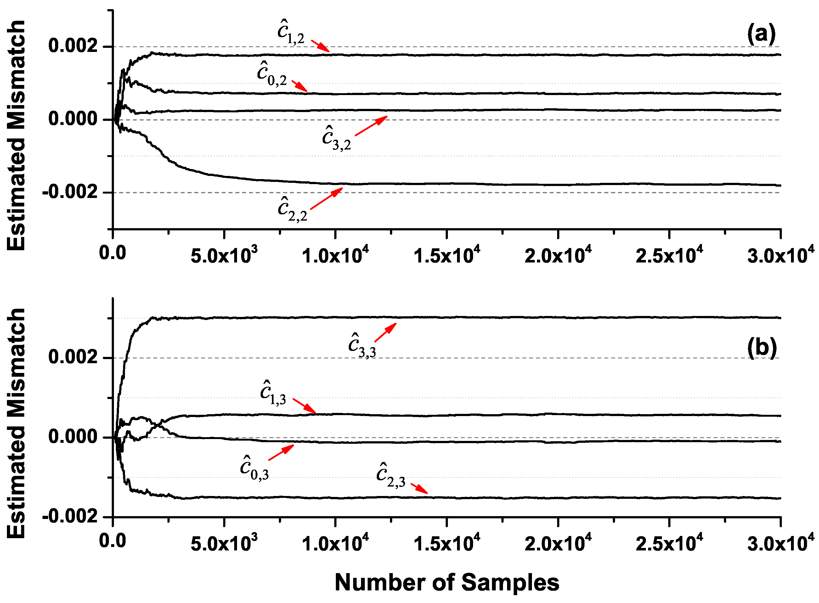
3.2. Mismatch Coefficients Estimation

In order to estimate the mismatch parameter $\mathit{C}$, the error signal in the input-free band is filtered out to drive the FxLMS algorithm. A high-pass finite impulse response (FIR) filter $h\left[n\right]$ is exploited in our design because the input-free band stemming from oversampling locates around the Nyquist frequency. However, the input-free band can be any where within the Nyquist band. The error signal filtered out by $h\left[n\right]$ is:

$$\epsilon \left[n\right]=y_c\left[n\right]\times h\left[n\right]={\overrightarrow{T}}_n^T\mathit{C}({\overrightarrow{P}}_{y\left[n\right]}^f+{\overrightarrow{R}}_{e\left[n\right]}^f)-{\overrightarrow{T}}_n^T\widehat{\mathit{C}}\left[n\right]{\overrightarrow{P}}_{y\left[n\right]}^f$$

(18)

where $x\left[n\right]$ is removed by the high pass filter $h\left[n\right]$ and:

$${\overrightarrow{R}}_{e\left[n\right]}^f={\overrightarrow{P}}_{x\left[n\right]}^f-{\overrightarrow{P}}_{y\left[n\right]}^f,$$

(19)

where:

$${\overrightarrow{P}}_{x\left[n\right]}^f=[x^2\left[n\right]\times h\left[n\right]x^3\left[n\right]\times h\left[n\right]\cdots x^L\left[n\right]\times h\left[n\right]]$$

(20)

and:

$${\overrightarrow{P}}_{y\left[n\right]}^f=[y^2\left[n\right]\times h\left[n\right]y^3\left[n\right]\times h\left[n\right]\cdots y^L\left[n\right]\times h\left[n\right]]$$

(21)

representing the high pass filtered version of the power terms ${\overrightarrow{P}}_{x\left[n\right]}$ and ${\overrightarrow{P}}_{y\left[n\right]}$, respectively.

The power of the cost function $\epsilon \left[n\right]$ is minimized when the estimated coefficient $\widehat{\mathit{C}}\left[n\right]=\mathit{C}$. Estimating the nonlinear parameter is an identification problem that can be solved by exploiting the FxLMS algorithm with the iteration function:

$$\widehat{\mathit{C}}[n+1]=\widehat{\mathit{C}}\left[n\right]+\mathsf{\mu }\mathsf{\epsilon }\left[n\right]({\overrightarrow{T}}_n{\overrightarrow{P}}_{y\left[n\right]}^{fT}).$$

(22)

The principle diagram of the nonlinear coefficients estimation is shown in Figure 5. The error reconstruction box in Figure 5 is the dashed box in Figure 4.

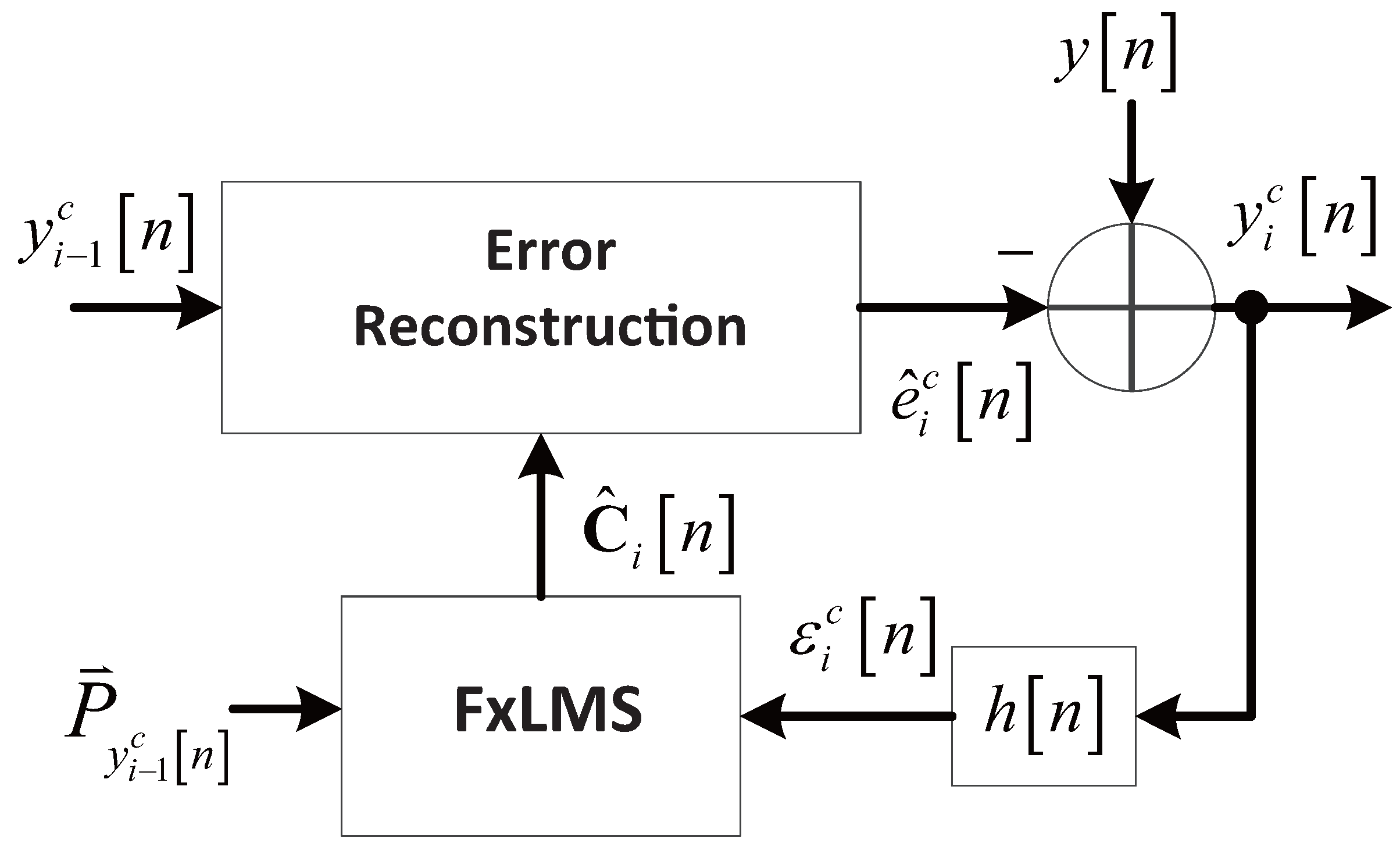
3.3. Cascade Calibration Structure

Exploiting the presented calibration structure and mismatch estimation method can suppress the error signal and improve the performance greatly in the weakly nonlinear systems. However, the calibration performance decreases with the increase of nonlinearity because the difference between $y\left[n\right]$ and $x\left[n\right]$ increases. A cascade calibration structure is employed to further improve the compensation performance.

Figure 6 shows the i-th stage calibration scheme of the cascade architecture. The calibrated output is denoted as $y_i^c\left[n\right](y_0^c\left[n\right]=y\left[n\right])$, which is expressed as:

$$y_i^c\left[n\right]=x\left[n\right]+{\overrightarrow{T}}_n^T(\mathit{C}-{\widehat{\mathit{C}}}_i\left[n\right]){\overrightarrow{P}}_{y_{i-1}^c\left[n\right]}+{\overrightarrow{T}}_n^T\mathit{C}({\overrightarrow{P}}_{x\left[n\right]}-{\overrightarrow{P}}_{y_{i-1}^c\left[n\right]}).$$

(23)

When the nonlinear parameter ${\widehat{\mathit{C}}}_i\left[n\right]$ converges to $\mathit{C}$, the residual error signal for the i-th stage output is:

$$e_i^r\left[n\right]={\overrightarrow{T}}_n^T\mathit{C}({\overrightarrow{P}}_{x\left[n\right]}-{\overrightarrow{P}}_{y_{i-1}\left[n\right]}).$$

(24)

Exploiting the fact that the power of error signal is much less than the power of input signal, the vector ${\overrightarrow{P}}_{y_{i-1}\left[n\right]}$ can be approximated by:

$${\overrightarrow{P}}_{y_{i-1}\left[n\right]}\approx {\overrightarrow{P}}_{x\left[n\right]}+{\overrightarrow{P}}_{x\left[n\right]}^{\prime }{e}_{i-1}^r\left[n\right]$$

(25)

where:

$${\overrightarrow{P}}_{x\left[n\right]}^{\prime }={[2x\left[n\right]3x^2\left[n\right]\cdots L{x}^{L-1}\left[n\right]]}^T.$$

(26)

Thus, the residual error of the i-th stage calibrated output is rewritten as:

$$e_i^r\left[n\right]\approx {\overrightarrow{T}}_n^T\mathit{C}{\overrightarrow{P}}_{x\left[n\right]}^{\prime }{e}_{i-1}^r\left[n\right].$$

(27)

In weakly nonlinear systems, $|{\overrightarrow{T}}_n^T\mathit{C}{\overrightarrow{P}}_{x\left[n\right]}^{\prime }|<1$ is guaranteed, i.e., $|e_i^r\left[n\right]|<|e_{i-1}^r\left[n\right]|$, which means the power of the residual error is decreasing using the cascade calibration structure. To be more specific, the magnitude of the residual error signal $e_{i-1}^r\left[n\right]$ and $e_i^r\left[n\right]$ is the order of $O({\left(c_{k,l}\right)}^i)$ and $O({\left(c_{k,l}\right)}^{i+1})$, respectively. If the nonlinearity-induced error is the only error source, the signal to noise and distortion ratio (SNDR) of the i-th stage calibrated output will decrease 20 dB per decade of the mismatch strength faster than the $(i-1)$-th stage output. This phenomenon is verified by the simulation result shown in Section 4.4.

4. Simulation Results

In this section, numerical simulation results are presented to demonstrate the efficacy and efficiency of the proposed method. The resolution of the simulated TIADCs is 12 bits unless otherwise stated, and the nonlinearities of the TIADCs are introduced utilizing polynomials. The high-pass filter is designed by the MATLAB function firpm, and the band edge of the filter is $0.8\mathsf{\pi }$.

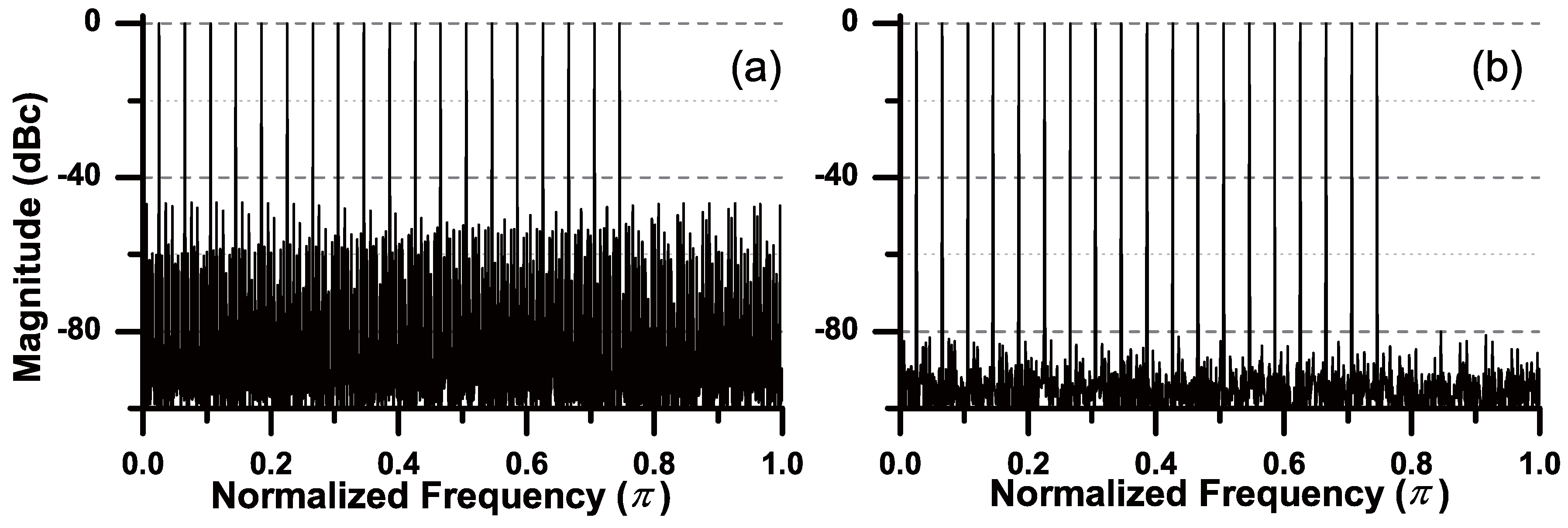
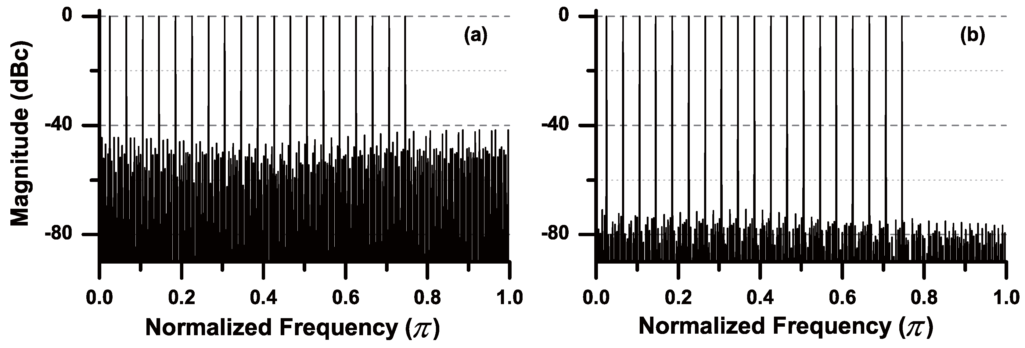
4.1. Calibration Performance with Different Numbers of Channels

Firstly, the calibration performance of the proposed method is verified in a 4-TIADC and an 8-TIADC to demonstrate that the proposed method works well in TIADCs with different numbers of channels. The polynomial coefficients for the 4-TIADC and the 8-TIADC are set as:

$$\begin{array}{c}{\overrightarrow{\mathsf{\alpha }}}_2={[0.001-0.0030.0040.001]}^T\hfill \\ {\overrightarrow{\mathsf{\alpha }}}_3={[0.002-0.005-0.0010.004]}^T\hfill \end{array}$$

(28)

and:

$$\begin{array}{c}{\overrightarrow{\mathsf{\alpha }}}_2={[0.001-0.0020.005-0.005-0.0020.0030.0040.002]}^T\hfill \\ {\overrightarrow{\mathsf{\alpha }}}_3={[0.001-0.003-0.0020.00.001-0.0040.0020.005]}^T\hfill \end{array}$$

(29)

respectively. A multi-tone signal composed of 19 sinusoids from DC to $0.745\mathsf{\pi }$ with a uniform amplitude is adopted as the input. The step size $\mathsf{\mu }$ is set to 0.1.

Example 1.

The spectra of 4-TIADC output without and with calibration are shown in Figure 7. As can be seen from the spectrum before calibration, the nonlinearity-induced error spurs spread over the entire Nyquist frequency band, although the input is band-limited to $0.745\mathsf{\pi }$. The SNDR and spurious-free dynamic range (SFDR) before calibration are 43.26 and 46.73 dB, while after calibration, the SNDR and SFDR increase to 75.48 and 80 dB, respectively.

The corresponding convergence curves are shown in Figure 8. The ideal nonlinear parameters calculated exploiting Equation (13) are ${\overrightarrow{c}}_2={[0.000750.00175-0.001750.00025]}^T$ and ${\overrightarrow{c}}_3={[00.0005-0.00150.003]}^T$. The estimated nonlinear parameters converge to the ideal parameters after about $1.0\times {10}^4$ samples as the figures show.

Example 2.

The input signal and simulation setting in this example are the same as in Example 1. The output spectra with and without calibration are shown in Figure 9. The error spurs are greatly suppressed after calibration as the figures show. The SNDR and SFDR before calibration are 38.51 and 40.82 dB, respectively, while after calibration, the SNDR and SFDR improve to 67.87 and 70.98 dB, respectively. The performance after calibration in this example is worse than the performance after calibration in Example 1. The reason is the SNDR before compensation is lower in this example, which means the difference between $y\left[n\right]$ and $x\left[n\right]$ is larger. Thus, the accuracy of error reconstruction decreases, and the calibration performance degrades.

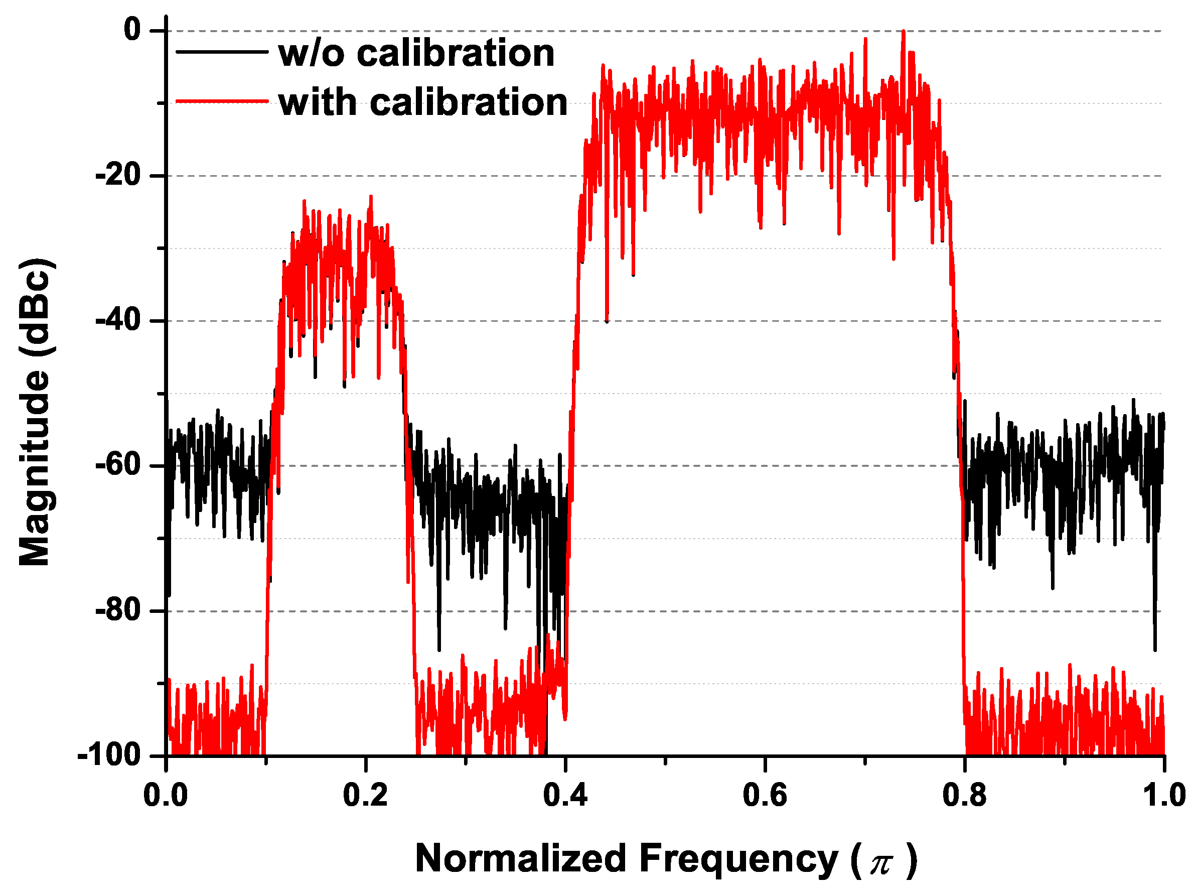
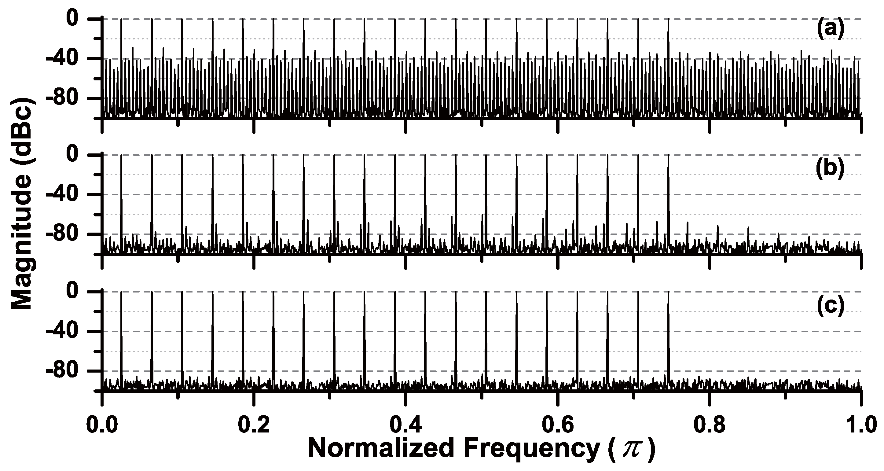
4.2. Calibration Performance with Different Input Signals

The compensation performance of the proposed algorithm with different input signals is presented in this subsection. The TIADC considered in this section is a 4-TIADC with the same nonlinear parameters as in Example 1.

Example 3.

In this example, a multi-band signal, which is generated by passing a zero-mean white noise through a dual pass-band filter, is fed into the 4-TIADC. Figure 10 shows the spectra of the multi-band signal with and without calibration. The noise level in the Nyquist band is improved from around −50 dB to less than −80 dB as the figure illustrates. From the figure, we can clearly see that the noise outside the passband of the high pass filter is also greatly suppressed. To quantify the performance improvement after calibration, we adopt the error vector magnitude (EVM) [25] as the figure of merit. The EVMs before and after calibration are −45.82 and −80.82 dB, respectively.

The convergence curves for 4-TIADC with multi-band noise input are shown in Figure 11. The estimated nonlinear parameters converge after about $1.0\times {10}^4$ samples, and they converge to the true nonlinear parameters as in Example 1.

Example 4.

In this example, we evaluate the calibration performance of our method in 4-TIADC with a band-pass multi-tone signal. A multi-tone signal with 11 sinusoids spanning from $0.305\mathsf{\pi }$ to $0.705\mathsf{\pi }$ is adopted. Figure 12 shows the spectra with and without calibration. The SNDR and SFDR before calibration are 39.6 and 43.87 dB, respectively, while the SNDR and SFDR after calibration are 74.79 and 81.33 dB, respectively.

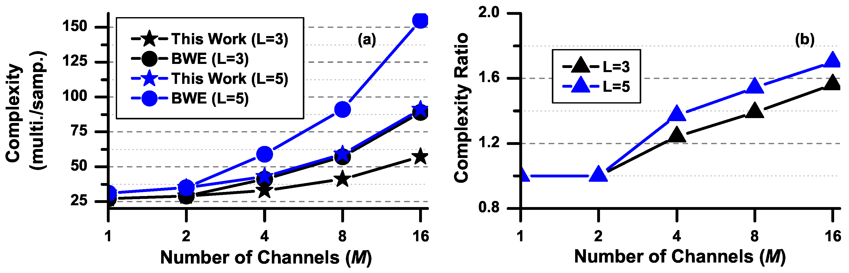
4.3. Computational Complexity

The complexity of the proposed method is analyzed in this section. The major advantage of our method over the approach proposed in [25] is that our method requires much less hardware resources and avoids the generation of sinusoidal modulation sequences $\frac{2}{M}cos(\frac{2\mathsf{\pi }}{M}nk)$ and $-\frac{2}{M}sin(\frac{2\mathsf{\pi }}{M}nk)$.

A brief comparison between this work and the BWE method proposed in [25] is shown in

Table 1. Comparison. BWE, bandwidth efficient.

Variable	This Work	BWE [25]
Number of channels	$M=1,2,4,8,\dots$	$M=1,2,3,\dots$
Bandwidth efficiency	$\mathsf{\eta }$	$\mathsf{\eta }$
Elements of modulation sequences	$\{1,-1\}$	$\{\frac{2}{M}cos(\frac{2\mathsf{\pi }}{M}nk),-\frac{2}{M}sin(\frac{2\mathsf{\pi }}{M}nk)\}$
Complexity (multipliers/sample)	$(M+1)(L-1)+\frac{N_{hp}}{2}+1$	$(2M+1)(L-1)+\frac{N_{hp}}{2}+1$

. One drawback of our method is that the number of channels is limited to the power of two, i.e., $M=1,2,4,8,\dots$, which is less general than the BWE method, as it can deal with the nonlinear mismatch problem in TIADCs with any integer number of channels. However, this drawback has little influence on the application of the proposed approach because the number of channels in a TIADC is usually the power of two in practice. The bandwidth efficiency property is maintained in the proposed method because the input-free band is utilized at the overall sampling frequency $F_s$.

The modulation sequences in our method only consist of 1 and −1, which are easy to process compared with the cumbersome modulation sequences $\frac{2}{M}cos(\frac{2\mathsf{\pi }}{M}nk)$ and $-\frac{2}{M}sin(\frac{2\mathsf{\pi }}{M}nk)$ adopted in [25]. Firstly, no specific circuit is required to generate modulation sequences composed of 1 and −1. By comparison, generating accurate sinusoidal signals requires a large amount of hardware resources. Secondly, no multiplier is required to implement the modulation by Hadamard sequences because it can be done by just changing the sign of the modulated signal. This means the multipliers used to multiply the modulation sequences are not required in our method. Apart from the resources to generate the modulation sequences, the number of multipliers consumed in the BWE method is $(2M+1)(L-1)+\frac{N_{hp}}{2}+1$, while our method only requires $(M+1)(L-1)+\frac{N_{hp}}{2}+1$ multipliers.

Figure 13 shows the number of multipliers consumed by the BWE method and our approach, as well as the ratio of the consumed multipliers. The order of the high-pass filter is 44; thus, 22 multipliers are needed exploiting the symmetric property of the FIR filter. As the figure shows, the difference between the multiplier consumed by the two methods increases with the increase of the number of channels and polynomial orders. The number of multipliers is the same for the two calibration methods in the case of single ADC and 2-TIADC, where 27 and 29 multipliers are consumed for $L=3$ and 31 and 35 multipliers for $L=5$. The difference of multiplier number and the complexity ratio is 32 and 1.56, respectively, for 16-TIADC with polynomial order $L=3$. The two numbers increase to 64 and 1.7 for 16-TIADC if the fifth order nonlinearities are considered.

Example 5.

Figure 14 reveals the performance improvement versus the order of the high-pass FIR filter. The simulation setup is the same as in Example 1. The SNDR and SFDR improvements increase rapidly with the increase of the high-pass filter orders when the order is less than 40. It can be inferred that a short FIR filter with about 40 taps is adequate for the application.

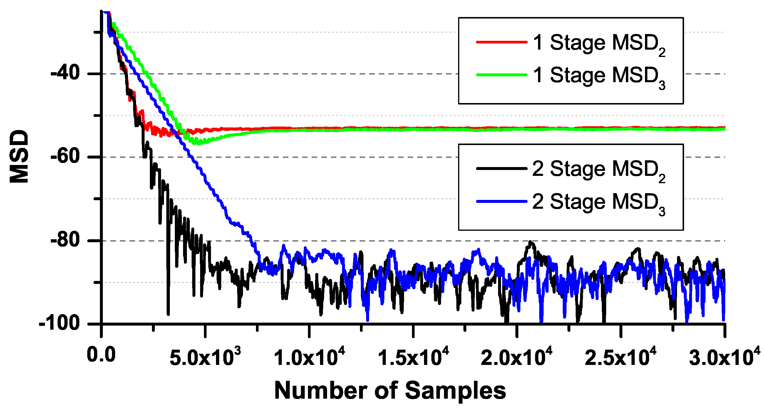
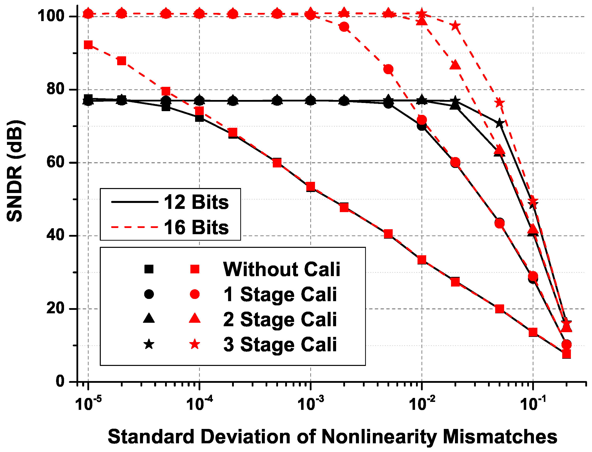
4.4. Performance of the Cascade Structure

Example 6.

The calibration performance of the cascade structure is illustrated in this section. Stronger nonlinearities are adopted in this example for better visualization. The nonlinear parameters in this example are:

$$\begin{array}{c}{\overrightarrow{\mathsf{\alpha }}}_2={[0.03-0.010.040.02]}^T\hfill \\ {\overrightarrow{\mathsf{\alpha }}}_3={[0.007-0.005-0.0050.004]}^T\hfill \end{array}$$

(30)

and the input signal is the same as in Example 1. TIADCs with 12-bit and 16-bit resolution are employed in this simulation to compare the calibration performance. Figure 15 shows the spectra of TIADC output without calibration, with one-stage calibration and with two-stage calibration. The SNDR and SFDR before calibration is 28.17 and 28.9 dB, respectively, while after one-stage and two-stage calibration, the two figures improve to 65.93, 60.65, 75.6 and 83.28 dB, respectively.

The mean square deviation (MSD) of the estimated parameters is adopted as the figure of merit for a clear view of the performance. The MSD is given by [25]:

$$MS{D}_l\left[n\right]=10\log 10(\sum _{k=0}^{M-1}{|c_{k,l}-{\widehat{c}}_{k,l}\left[n\right]|}^2).$$

(31)

Figure 16 shows the MSD curves for one-stage calibration and two-stage calibration. It is inferred from the figure that the accuracy of nonlinear parameters’ estimation is greatly improved exploiting the two-stage calibration structure.

Figure 17 shows the SNDR of the TIADC output with and without calibration versus the standard deviation of nonlinearity mismatches. The nonlinear parameters ${\overrightarrow{\mathsf{\alpha }}}_2$ and ${\overrightarrow{\mathsf{\alpha }}}_3$ are set as independent random variables with a Gaussian distribution. The results are obtained by performing 1000 Monte Carlo simulations. The input signal is the same as in Example 1. The SNDR decreases by about 20 dB per decade of the nonlinear strength for the uncalibrated signal. After the i stage calibration, the dropping rate increases to about $20\times i$ per decade of the nonlinear strength, which corresponds with the analysis in Section 3.3.

5. Conclusions

This paper introduces a blind adaptive method to compensate for the nonlinear mismatches in M-TIADCs. In our method, the nonlinearity-induced error signal is reconstructed by the proposed multiplier Hadamard transform (MHT) structure, and the nonlinear parameters are estimated by the FxLMS algorithm. The proposed MHT structure exploits the binary Hadamard sequences instead of the sinusoidal sequences to modulate the TIADC output. Compared with the method based on sinusoidal sequences, our method avoids the complicated circuits to generate sinusoidal sequences. Moreover, the number of multipliers is greatly reduced benefiting from the simple implementation of Hadamard sequence modulation.

References

1. Bonnetat, A.; Hode, J.M.; Ferre, G.; Dallet, D. An adaptive all-digital blind compensation of dual-TIADC frequency-response mismatch based on complex signal correlations. IEEE Trans. Circ. Syst. II Express Briefs 2015, 62, 821–825. [Google Scholar] [CrossRef]
2. Bonnetat, A.; Hode, J.M.; Ferre, G.; Dallet, D. Correlation-based frequency-response mismatch compensation of quad-TIADC using real samples. IEEE Trans. Circ. Syst. II Express Briefs 2015, 62, 746–750. [Google Scholar] [CrossRef]
3. Singh, S.; Anttila, L.; Epp, M.; Schlecker, W.; Valkama, M. Frequency response mismatches in 4-channel time-interleaved ADCs: Analysis, blind identification, and correction. IEEE Trans. Circ. Syst. I Regul. Pap. 2015, 62, 2268–2279. [Google Scholar] [CrossRef]
4. Singh, S.; Anttila, L.; Epp, M.; Schlecker, W.; Valkama, M. Analysis, blind identification, and correction of frequency response mismatch in two-channel time-interleaved ADCs. IEEE Trans. Microw. Theory Tech. 2015, 63, 1721–1734. [Google Scholar] [CrossRef]
5. Singh, S.; Valkama, M.; Epp, M.; Schlecker, W. Digitally enhanced wideband I/Q downconversion receiver with 2-channel time-interleaved ADCs. IEEE Trans. Circ. Syst. II Express Briefs 2016, 63, 29–33. [Google Scholar] [CrossRef]
6. Singh, S.; Valkama, M.; Epp, M.; Schlecker, W. Frequency response mismatch analysis in time-interleaved analog I/Q processing and ADCs. IEEE Trans. Circ. Syst. II Express Briefs 2015, 62, 608–612. [Google Scholar] [CrossRef]
7. Li, J.; Wu, S.; Liu, Y.; Ning, N.; Yu, Q. A digital timing mismatch calibration technique in time-interleaved ADCs. IEEE Trans. Circ. Syst. II Express Briefs 2014, 61, 486–490. [Google Scholar] [CrossRef]
8. Matsuno, J.; Yamaji, T.; Furuta, M.; Itakura, T. All-digital background calibration technique for time-interleaved ADC using pseudo aliasing signal. IEEE Trans. Circ. Syst. I Regul. Pap. 2013, 60, 1113–1121. [Google Scholar] [CrossRef]
9. Zou, Y.X.; Xu, X.J. Blind timing skew estimation using source spectrum sparsity in time-interleaved ADCs. IEEE Trans. Instrum. Meas. 2012, 61, 2401–2412. [Google Scholar] [CrossRef]
10. Saleem, S.; Vogel, C. Adaptive blind background calibration of polynomial-represented frequency response mismatches in a two-channel time-interleaved ADC. IEEE Trans. Circ. Syst. I Regul. Pap. 2011, 58, 1300–1310. [Google Scholar] [CrossRef]
11. Tsui, K.M.; Chan, S.C. New iterative framework for frequency response mismatch correction in time-interleaved ADCs: Design and performance analysis. IEEE Trans. Instrum. Meas. 2011, 60, 3792–3805. [Google Scholar] [CrossRef] [Green Version]
12. Divi, V.; Wornell, G.W. Blind calibration of timing skew in time-interleaved analog-to-digital converters. IEEE J. Sel. Top. Signal Process. 2009, 3, 509–522. [Google Scholar] [CrossRef]
13. Johansson, H. A polynomial-based time-varying filter structure for the compensation of frequency-response mismatch errors in time-interleaved ADCs. IEEE J. Sel. Top. Signal Process. 2009, 3, 384–396. [Google Scholar] [CrossRef]
14. Satarzadeh, P.; Levy, B.C.; Hurst, P.J. Adaptive semiblind calibration of bandwidth mismatch for two-channel time-interleaved ADCs. IEEE Trans. Circ. Syst. I Regul. Pap. 2009, 56, 2075–2088. [Google Scholar] [CrossRef]
15. Vogel, C.; Mendel, S. A flexible and scalable structure to compensate frequency response mismatches in time-interleaved ADCs. IEEE Trans. Circ. Syst. I Regul. Pap. 2009, 56, 2463–2475. [Google Scholar] [CrossRef]
16. Huang, S.; Levy, B.C. Blind calibration of timing offsets for four-channel time-interleaved ADCs. IEEE Trans. Circ. Syst. I Regul. Pap. 2007, 54, 863–876. [Google Scholar] [CrossRef]
17. Huang, S.; Levy, B.C. Adaptive blind calibration of timing offset and gain mismatch for two-channel time-interleaved ADCs. IEEE Trans. Circ. Syst. I Regul. Pap. 2006, 53, 1278–1288. [Google Scholar] [CrossRef]
18. Tsai, T.H.; Hurst, P.J.; Lewis, S.H. Bandwidth mismatch and its correction in time-interleaved analog-to-digital converters. IEEE Trans. Circ. Syst. II Express Briefs 2006, 53, 1133–1137. [Google Scholar] [CrossRef]
19. Wang, C.Y.; Wu, J.T. A background timing-skew calibration technique for time-interleaved analog-to-digital converters. IEEE Trans. Circ. Syst. II Express Briefs 2006, 53, 299–303. [Google Scholar] [CrossRef]
20. Jamal, S.M.; Fu, D.; Singh, M.P.; Hurst, P.J.; Lewis, S.H. Calibration of sample-time error in a two-channel time-interleaved analog-to-digital converter. IEEE Trans. Circ. Syst. I Regul. Pap. 2004, 51, 130–139. [Google Scholar] [CrossRef]
21. Kurosawa, N.; Kobayashi, H.; Kobayashi, K. Channel linearity mismatch effects in time-interleaved ADC systems. IEICE Trans. Fundam. Electron. Commun. Comput. Sci. 2002, 85, 749–756. [Google Scholar]
22. Simoes, J.B.; Landeck, J.; Correia, C.M.B.A. Nonlinearity of a data-acquisition system with interleaving/multiplexing. IEEE Trans. Instrum. Meas. 1997, 46, 1274–1279. [Google Scholar] [CrossRef]
23. Goodman, J.; Miller, B.; Herman, M.; Raz, G.; Jackson, J. Polyphase nonlinear equalization of time-interleaved analog-to-digital converters. IEEE J. Sel. Top. Signal Process. 2009, 3, 362–373. [Google Scholar] [CrossRef]
24. Centurelli, F.; Monsurro, P.; Trifiletti, A. Improved digital background calibration of time-interleaved pipeline A/D converters. IEEE Trans. Circ. Syst. II Express Briefs 2013, 60, 86–90. [Google Scholar] [CrossRef]
25. Wang, Y.; Johansson, H.; Xu, H.; Diao, J. Bandwidth-efficient calibration method for nonlinear errors in M-channel time-interleaved ADCs. Analog Integr. Circ. Signal Process. 2016, 86, 275–288. [Google Scholar] [CrossRef]
26. Wang, Y.; Hui, X.; Johansson, H.; Zhaolin, S.; Wikner, J. Digital estimation and compensation method for nonlinearity mismatches in time-interleaved analog-to-digital converters. Digit. Signal Process. 2015, 41, 130–141. [Google Scholar] [CrossRef]
27. Wang, Y.; Johansson, H.; Hui, X.; Zhaolin, S. Joint blind calibration for mixed mismatches in two-channel time-interleaved ADCs. IEEE Trans. Circ. Syst. I Regul. Pap. 2015, 62, 1508–1517. [Google Scholar] [CrossRef]
28. Wang, Y.; Johansson, H.; Xu, H. Adaptive background estimation for static nonlinearity mismatches in two-channel TIADCs. IEEE Trans. Circ. Syst. II Express Briefs 2015, 62, 226–230. [Google Scholar] [CrossRef]
29. Vogel, C.; Kubin, G. Modeling of time-interleaved ADCs with nonlinear hybrid filter banks. AEU Int. J. Electron. Commun. 2005, 59, 288–296. [Google Scholar] [CrossRef]
30. Asami, K.; Suzuki, T.; Miyajima, H.; Taura, T.; Kobayashi, H. Technique to improve the performance of time-interleaved AD converters with mismatches of non-linearity. IEICE Trans. Fundam. Electron. Commun. Comput. Sci. 2009, 92, 374–380. [Google Scholar] [CrossRef]
31. Vogel, C.; Kubin, G. Analysis and compensation of nonlinearity mismatches in time-interleaved ADC arrays. In Proceedings of the 2004 International Symposium on Circuits and Systems, Vancouver, BC, Canada, 23–26 May 2004; Volume 1, pp. I-593–I-596.
32. Liu, H.; Xu, H. A calibration method for frequency response mismatches in M-channel time-interleaved analog-to-digital converters. IEICE Electron. Express 2016. [Google Scholar] [CrossRef]
Figure 1. (a) A time-interleaved analog-to-digital converter (ADC) consists of M sub-ADCs; (b) timing diagram of the sampling clocks. MUX, Multiplexer; CLK, Clock.
Applsci 06 00362 g001
Figure 2. Nonlinear mismatches in the M-time-interleaved analog-to-digital converter (TIADC) are interpreted as the sum of a series of gain-mismatched M-TIADCs.
Applsci 06 00362 g002
Figure 3. (a) Model of M-TIADC with nonlinear mismatches; (b) the detail of the Hadamard transform (HT) block.
Applsci 06 00362 g003
Figure 4. Calibration structure for nonlinear mismatches in M-TIADCs. The HT block is the same as Figure 3b, where the parameters c k , l are replaced by the estimated parameters c ^ k , l [ n ] .
Applsci 06 00362 g004
Figure 5. Adaptive calibration structure exploiting the filtered-X least mean square (FxLMS) algorithm.
Applsci 06 00362 g005
Figure 6. The structure of the i-th stage calibration structure.
Applsci 06 00362 g006
Figure 7. The spectra of 4-TIADC output (a) before and (b) after calibration.
Applsci 06 00362 g007
Figure 8. The convergence behavior of the estimated parameters c ^ k , l [ n ] . (a) Second order nonlinear parameters; (b) third order nonlinear parameters.
Applsci 06 00362 g008
Figure 9. The spectra of 8-TIADC (a) before and (b) after calibration.
Applsci 06 00362 g009
Figure 10. The spectra of 4-TIADC output with and without calibration for dual band noise input.
Applsci 06 00362 g010
Figure 11. The convergence behavior of the estimated parameters c ^ k , l [ n ] for dual band noise input. (a) Second order nonlinear parameters; (b) third order nonlinear parameters.
Applsci 06 00362 g011
Figure 12. The spectra of 4-TIADC output (a) before and (b) after calibration for bandpass multi-tone sinusoidal signal input.
Applsci 06 00362 g012
Figure 13. (a) Complexity and (b) complexity ratio under different numbers of channels and orders of the nonlinearity. BWE, bandwidth efficient.
Applsci 06 00362 g013
Figure 14. Performance (signal to noise and distortion ratio (SNDR) and spurious-free dynamic range (SFDR)) improvement under different orders of the high pass filter.
Applsci 06 00362 g014
Figure 15. The spectra of 4-TIADC output. (a) Without calibration; (b) one-stage calibration; (c) two-stage calibration.
Applsci 06 00362 g015
Figure 16. The mean square deviation (MSD) of one-stage calibration and two-stage calibration.
Applsci 06 00362 g016
Figure 17. The SNDR of calibrated 4-TIADC output with different strengths of nonlinear mismatches.
Applsci 06 00362 g017