Benefits and Impact of Joint Metric of AOA/RSS/TOF on Indoor Localization Error

Abstract

The emerging techniques in the Fifth Generation (5G) communication system, like the millimeter-Wave (mmWave) and massive Multiple Input Multiple Output (MIMO), make it possible to measure the Angle-Of-arrival (AOA), Receive Signal Strength (RSS) and Time-Of-flight (TOF) by using various types of mobile devices. At the same time, there is always significant interest in the high-precision localization techniques based on the joint metric of AOA/RSS/TOF, which enable one to overcome the drawback of the single metric-based localization. Motivated by this concern, we rely on the Cramer–Rao Lower Bound (CRLB) to analyze the localization errors of RSS/AOA, RSS/TOF, AOA/TOF and the Joint Metric of AOA/RSS/TOF (JMART)-based localization. The error bounds derived in this paper can be selected as the benchmarking results to evaluate the indoor localization performance. Finally, extensive simulations are conducted to support our claim.

1. Introduction

Indoor localization has gained considerable attention over the past decade due to the significant development of ubiquitous Location-Based Services (LBSs). The popular Global Positioning System (GPS) [1] has been recognized as a success for outdoor localization under the Line-Of-Sight (LOS) propagation property, whereas extending the GPS to the indoor environment with the None-Line-Of-Sight (NLOS) propagation property faces a serious challenge due to the irregular signal fading and multi-path interference. An alternative approach to address this challenge is the site survey-based location fingerprinting approach, which is based on the construction of a database of location fingerprints collected at Reference Points (RPs). In this case, the target locations are estimated by mapping the newly-collected Received Signal Strengths (RSSs) against the pre-constructed database of location fingerprints [2,3,4,5]. However, the existence of the multi-path effect, wall sheltering and channel interference still results in the significant temporal and spatial variation of RSSs and consequently leads to the increase of localization error [6].

The emerging techniques in the Fifth Generation (5G) communication system enable us to measure the Angle-Of-Arrive (AOA), RSS and Time-Of-Flight (TOF) with various types of mobile devices [7]. Then, the indoor localization by using the Joint Metric of AOA/RSS/TOF (JMART) will be preferred compared to the conventional metric by using the AOA, RSS or TOF solely [8,9,10,11], which is more vulnerable to the environmental changes.

The motivation of this paper is to investigate the benefits and impact of the JMART on the indoor localization error. In concrete terms, we use the Fisher Information Matrix (FIM) [12,13,14] to measure the information of the JMART and then rely on the Cramer–Rao Lower Bound (CRLB) [15] to solve the corresponding unbiased localization problem [16].

The rest of this paper is structured as follows. We survey some related work in Section 2. In Section 3, we derive the error bound by selecting the conventional AOA, RSS or TOF solely as the metric, as well as investigate the impact of the metrics of RSS/AOA, RSS/TOF and AOA/TOF on indoor localization error, which helps to derive the error bound by the JMART. The extensive simulations are provided in Section 4 to verify the benefits of the JMART. Finally, we conclude the paper and give the future directions in Section 5.

2. Related Works

Depending on the ranging metric, the existing indoor localization solutions in wireless networks can be commonly classified into three categories, AOA-based, RSS-based and TOF-based indoor localization [17]. The performance of RSS-based indoor localization highly depends on the physical layout, propagation loss and channel interference, while the NLOS propagation property may seriously degrade the performance of AOA-based and TOF-based indoor localization due to the difficulty of detecting the direct signal path and measuring the time of flight of the signal, respectively [18]. Thus, the metric by using the AOA, RSS or TOF solely is vulnerable to environmental changes. To solve this problem, the authors in [19] proposed to use the metric of RSS/TOF to conduct the localization based on the determining likelihood function, which is used to depict the relations between the measurements and distances. The authors in [20] presented a scheme in which the metrics of RSS and AOA are integrated to restrain the NLOS fading. The authors in [21] developed an efficient approach to localize the mobile sensors using the metrics of TOF and AOA with the help of multiple seeds adopted to obtain adequate observations.

There are batches of studies analyzing the error bound of localization by using the FIM. The authors in [22] selected the CRLB to investigate the localization error by performing the unbiased Gaussian range estimation based on the metric of AOA. In [23], the authors proposed to use the information inequality-based Position Error Bound (PEB) to analyze the error performance of TOF-based cooperative localization. The authors in [24] investigated the impact of the bandwidth and sampling rate of the receiver on the accuracy of the radar localization systems based on the Cramer–Rao bounds of the TOF and TDOA. In [25], the authors derived the error bound of the RSS-based localization for the uncertain network topology by using the Fisher information and Cramer–Rao inequality. Similarly, the authors in [26] analyzed the CRLB of the localization by selecting the Signal Strength Difference (SSD) as the location fingerprint. In addition, the bound of localization error helps greatly in designing effective localization algorithms, as well as providing valuable suggestions for the construction of superior localization systems by revealing the error trends, which are associated with the network deployment. In [27], the authors quantifies via the Cramer–Rao bound on location estimators, which use measured TOF or RSS. The authors in [28] realized the highly-accurate positioning of the sensors by using the metrics of RSS and TOF. Different from the literature above, which analyzed the unbiased localization problem, the authors in [29] analyzed the impact of various parameters in system design, as well as the biased measurements on positioning performance and meanwhile derived an asymptotic expression for positioning mean-square error in the network-based multilateral localization system. The mathematical analysis in [29] is based on the CRLB and maximum likelihood theory. Furthermore, the authors in [30] studied the deterministic CRLBs for the estimation of the specular multipath parameters and target locations in an asynchronous direct sequence code division multiple access system, which operates over the specular multipath fading channel.

However, the existing literature mainly focused on the analysis of the localization error bound by selecting the AOA, RSS or TOF solely as the metric. Different from these, we investigate the error bound with respect to the JMART used for the indoor localization. The most important contribution of this paper is to derive the error bounds by using the AOA, RSS, TOF and JMART respectively for the unbiased localization problem. To achieve this goal, on the one hand, we use the deviation $\mathsf{\sigma }$ to approximately describe the multipath effect, which is also used in [22,23,24,25,26]. On the other hand, our work aims to be applied in the future 5G communication system, in which many emerging techniques, like the millimeter-wave and massive Multiple Input Multiple Output (MIMO), make it possible to estimate the signal parameters (such as the AOA or TOF) of multipath signals with high resolution. In addition, the analytical result of the error bound can be derived as a function of the number of Access Points (APs), RSS distributions and noise power.

3. Error Bound Analysis

In this section, we will derive the error bounds of localization by using the single measurement of RSS, TOF or AOA, double measurements of RSS/AOA, RSS/TOF or AOA/TOF and the JMART based on the FIM.

Let $\widehat{{\mathsf{\theta }}_i}=\left(\widehat{x_i}\right.,{\left.\widehat{y_i}\right)}^{\mathrm{T}}$ be the unbiased estimate of the i-th real location ${\mathsf{\theta }}_i=\left(x_i\right.,{\left.y_i\right)}^{\mathrm{T}}$. Then, the covariance matrix with respect to $\widehat{{\mathsf{\theta }}_i}$ is calculated by:

$$\mathrm{E}\left[\left(\widehat{{\mathsf{\theta }}_i}-{\mathsf{\theta }}_i\right){\left(\widehat{{\mathsf{\theta }}_i}-{\mathsf{\theta }}_i\right)}^{\mathrm{T}}\right]=\left[\begin{array}{c}{\mathsf{\sigma }}_{\widehat{x_i}}^2\hfill \\ {\mathsf{\sigma }}_{\widehat{y_i}\widehat{x_i}}^2\hfill \end{array}\right.\left.\begin{array}{c}{\mathsf{\sigma }}_{\widehat{x_i}\widehat{y_i}}^2\hfill \\ {\mathsf{\sigma }}_{\widehat{y_i}}^2\hfill \end{array}\right]$$

(1)

where ${\mathsf{\sigma }}_{\widehat{x_i}}^2$ and ${\mathsf{\sigma }}_{\widehat{y_i}}^2$ are the Mean Square Errors (MSEs) with respect to $\widehat{x_i}$ and $\widehat{y_i}$. ${\mathsf{\sigma }}_{\widehat{x_i}\widehat{y_i}}^2$ and ${\mathsf{\sigma }}_{\widehat{y_i}\widehat{x_i}}^2$ are the covariance between $\widehat{x_i}$ and $\widehat{y_i}$ and between $\widehat{y_i}$ and $\widehat{x_i}$, respectively. The notations “var”, “E” and “T” stand for the variance, Expectation and Transpose operations. If $\widehat{{\mathsf{\theta }}_i}$ is calculated from the unbiased estimate of the measurement (e.g., RSS, TOF or AOA) at the i-th real location ${\mathbf{m}}_i$, we can use the FIM to construct the relations below to present the lower bound of the variance of $\widehat{{\mathsf{\theta }}_i}$.

$$\mathrm{var}\left[\widehat{{\mathsf{\theta }}_i}\right]\ge \mathrm{E}{\left\{-\frac{{\partial }^2\ln f_{{\mathsf{\theta }}_i}\left({\mathbf{m}}_i\right)}{\partial {{\mathsf{\theta }}_i}^2}\right\}}^{-1}=J{\left({\mathsf{\theta }}_i\right)}^{-1}$$

(2)

where $f_{{\mathsf{\theta }}_i}\left({\mathbf{m}}_i\right)$ and $J\left({\mathsf{\theta }}_i\right)$ are the Probability Distribution Function (PDF) of ${\mathbf{m}}_i$ and FIM with respect to ${\mathsf{\theta }}_i$. Using the concept of the score function in [31], we obtain that:

$$U\left({\mathsf{\theta }}_i\right)=\frac{\partial }{\partial {\mathsf{\theta }}_i}\ln f_{{\mathsf{\theta }}_i}\left({\mathbf{m}}_i\right)$$

(3)

where $U\left({\mathsf{\theta }}_i\right)$ is the score function with respect to ${\mathsf{\theta }}_i$.

For any ${\mathsf{\theta }}_i$ under the regularity condition [31], if $f_{{\mathsf{\theta }}_i}\left({\mathbf{m}}_i\right)$ belongs to the exponential family, we have:

$$\mathrm{E}\left[U\left({\mathsf{\theta }}_i\right)\right]=\mathrm{E}\left[\frac{\partial }{\partial {\mathsf{\theta }}_i}\ln f_{{\mathsf{\theta }}_i}\left({\mathbf{m}}_i\right)\right]=\mathrm{E}\left[\frac{1}{f_{{\mathsf{\theta }}_i}\left({\mathbf{m}}_i\right)}·\frac{\partial }{\partial {\mathsf{\theta }}_i}{f}_{{\mathsf{\theta }}_i}\left({\mathbf{m}}_i\right)\right]=0,$$

(4)

Based on [26], we obtain that $J\left({\mathsf{\theta }}_i\right)=-\mathrm{E}\left\{\frac{U\left({\mathsf{\theta }}_i\right)}{\partial {\mathsf{\theta }}_i}\right\}=-\mathrm{E}{\left[\frac{\partial \ln f_{{\mathsf{\theta }}_i}\left({\mathbf{m}}_i\right)}{\partial {\mathsf{\theta }}_i}\right]}^2$. Let:

$$J\left({\mathsf{\theta }}_i\right)=\left[\begin{array}{c}{J}_{x_i{x}_i}\left({\mathbf{m}}_i\right)\hfill \\ J_{y_i{x}_i}\left({\mathbf{m}}_i\right)\hfill \end{array}\right.\left.\begin{array}{c}{J}_{x_i{y}_i}\left({\mathbf{m}}_i\right)\hfill \\ J_{y_i{y}_i}\left({\mathbf{m}}_i\right)\hfill \end{array}\right]$$

(5)

where $\left\{\begin{array}{c}{J}_{x_i{x}_i}\left({\mathbf{m}}_i\right)=-\mathrm{E}\left\{\frac{{\partial }^2}{\partial {x_i}^2}\ln f_{{\mathsf{\theta }}_i}\left({\mathbf{m}}_i\right)\right\}\hfill \\ J_{x_i{y}_i}\left({\mathbf{m}}_i\right)=-\mathrm{E}\left\{\frac{{\partial }^2}{\partial x_i\partial y_i}\ln f_{{\mathsf{\theta }}_i}\left({\mathbf{m}}_i\right)\right\}\hfill \\ J_{y_i{x}_i}\left({\mathbf{m}}_i\right)=-\mathrm{E}\left\{\frac{{\partial }^2}{\partial y_i\partial x_i}\ln f_{{\mathsf{\theta }}_i}\left({\mathbf{m}}_i\right)\right\}\hfill \\ J_{y_i{y}_i}\left({\mathbf{m}}_i\right)=-\mathrm{E}\left\{\frac{{\partial }^2}{\partial {y_i}^2}\ln f_{{\mathsf{\theta }}_i}\left({\mathbf{m}}_i\right)\right\}.\hfill \end{array}\right.$

Based on (2), since:

$$J{\left({\mathsf{\theta }}_i\right)}^{-1}=\frac{1}{\left|J\left({\mathsf{\theta }}_i\right)\right|}·\left[\begin{array}{c}{J}_{y_i{y}_i}\left({\mathbf{m}}_i\right)\hfill \\ -J_{x_i{y}_i}\left({\mathbf{m}}_i\right)\hfill \end{array}\right.\left.\begin{array}{c}-J_{y_i{x}_i}\left({\mathbf{m}}_i\right)\hfill \\ J_{x_i{x}_i}\left({\mathbf{m}}_i\right)\hfill \end{array}\right],$$

(6)

where $\left|J\left({\mathsf{\theta }}_i\right)\right|=J_{x_i{x}_i}\left({\mathbf{m}}_i\right)J_{y_i{y}_i}\left({\mathbf{m}}_i\right)-J_{x_i{y}_i}{\left({\mathbf{m}}_i\right)}^2$, we calculate that:

$$\left\{\begin{array}{c}{\mathsf{\sigma }}_{\widehat{x_i}}^2=\mathrm{E}{\left(\widehat{x_i}-x_i\right)}^2\ge \frac{J_{y_i{y}_i}\left({\mathbf{m}}_i\right)}{\left|J\left({\mathsf{\theta }}_i\right)\right|}\hfill \\ {\mathsf{\sigma }}_{\widehat{y_i}}^2=\mathrm{E}{\left(\widehat{y_i}-y_i\right)}^2\ge \frac{J_{x_i{x}_i}\left({\mathbf{m}}_i\right)}{\left|J\left({\mathsf{\theta }}_i\right)\right|}\hfill \end{array}\right.$$

(7)

Then, by selecting the RSS as the metric for the localization, the CRLB with respect to ${\mathsf{\theta }}_i$ under m APs condition equals:

$$V_m\left({\mathbf{m}}_i\right)=\frac{J_{x_i{x}_i}\left({\mathbf{m}}_i\right)+J_{y_i{y}_i}\left({\mathbf{m}}_i\right)}{\left|J\left({\mathsf{\theta }}_i\right)\right|}$$

(8)

Therefore, the average localization error bound for the target environment, $V_{\mathrm{ave}}\left({\mathbf{m}}_i\right)$, is:

$$V_{\mathrm{ave}}\left({\mathbf{m}}_i\right)=\frac{1}{n}\sum _{i=1}^n{V}_m\left({\mathbf{m}}_i\right)$$

(9)

where n is the number of real locations in the target environment.

3.1. Metric of Single Measurement

3.1.1. Metric of RSS

In this section, we select the metric of RSS to conduct the indoor localization. For simplicity, we select the COST231 model to depict the propagation property, which is also considered in [32,33] as a good compromise among practicability, precision and simplicity. The COST231 model is shown in (10).

$$\widehat{P_{ik}}=P\left(d_0\right)-10\mathsf{\beta }{\log }_{10}\left(\frac{d_{ik}}{d_0}\right)-P_w-{\chi }_1$$

(10)

where $\widehat{P_{ik}}$ and $P\left(d_0\right)$ are the RSSs received (in dBm) at the locations with $d_{ik}$ and $d_0$ meters, respectively, from the AP. $d_0$ and $d_{ik}$ are the reference distance and distance between the k-th AP, $\left(x_k\right.,\left.y_k\right)$ and ${\mathsf{\theta }}_i$. $\mathsf{\beta }$ is the path loss exponent. $P_w$ is the path loss caused by the walls. ${\chi }_1$ is a random variable following the Gaussian distribution with the mean zero and variance ${{\mathsf{\sigma }}_1}^2$, $N\left(0,{{\mathsf{\sigma }}_1}^2\right)$. The PDF of ${\mathit{P}}_{ik}$ with respect to ${\mathsf{\theta }}_i$ is:

$$f_{{\mathsf{\theta }}_i}\left({\mathit{P}}_{ik}\right)=\prod _{k=1}^m\frac{1}{\sqrt{2\mathsf{\pi }}{\mathsf{\sigma }}_1}\exp \left(-\frac{{{\mathsf{\xi }}_{i1}}^2}{2{{\mathsf{\sigma }}_1}^2}\right)$$

(11)

where ${\mathsf{\xi }}_{i1}=\widehat{P_{ik}}-P\left(d_0\right)+10\mathsf{\beta }{\log }_{10}\left(d_{ik}\right)+P_{wf}$. m is the AP number. Based on (5), we can calculate that:

$$\left\{\begin{array}{c}J\left({\mathsf{\theta }}_i\right)=\left[\begin{array}{c}{J}_{xx}\left(\mathrm{RSS}\right)\hfill \\ J_{yx}\left(\mathrm{RSS}\right)\hfill \end{array}\right.\left.\begin{array}{c}{J}_{xy}\left(\mathrm{RSS}\right)\hfill \\ J_{yy}\left(\mathrm{RSS}\right)\hfill \end{array}\right]\hfill \\ J_{xx}\left(\mathrm{RSS}\right)={\mathsf{\rho }}_1{\displaystyle \sum _{k=1}^m}{\left[\frac{\cos {\mathsf{\alpha }}_{ik}}{d_{ik}}\right]}^2\hfill \\ J_{xy}\left(\mathrm{RSS}\right)=J_{yx}\left(\mathrm{RSS}\right)={\mathsf{\rho }}_1{\displaystyle \sum _{k=1}^m}\frac{\sin {\mathsf{\alpha }}_{ik}\cos {\mathsf{\alpha }}_{ik}}{{d_{ik}}^2}\hfill \\ J_{yy}\left(\mathrm{RSS}\right)={\mathsf{\rho }}_1{\displaystyle \sum _{k=1}^m}{\left[\frac{\sin {\mathsf{\alpha }}_{ik}}{d_{ik}}\right]}^2\hfill \end{array}\right.$$

(12)

where ${\mathsf{\alpha }}_{ik}=\arctan \frac{\left|y_i-y_k\right|}{\left|x_i-x_k\right|}$. ${\mathsf{\rho }}_1={\left(\frac{10\mathsf{\beta }}{{\mathsf{\sigma }}_1\ln 10}\right)}^2$. The geometric relationship between the locations $\left(x_i,y_i\right)$ and $\left(x_k,y_k\right)$ is shown in Figure 1.

Therefore, based on (8), the localization error bound by using the metric of RSS with respect to ${\mathsf{\theta }}_i$ equals:

$$\begin{array}{cc}{V}_m\left(\mathrm{RSS}\right)\hfill & =\frac{J_{yy}\left(\mathrm{RSS}\right)+J_{xx}\left(\mathrm{RSS}\right)}{J_{xx}\left(\mathrm{RSS}\right)·J_{yy}\left(\mathrm{RSS}\right)-{J_{xy}}^2\left(\mathrm{RSS}\right)}\hfill \\ & =\frac{1}{{\mathsf{\rho }}_1}·\frac{{\displaystyle \sum _{k=1}^m}{\left[\frac{\cos {\mathsf{\alpha }}_{ik}}{d_{ik}}\right]}^2+{\displaystyle \sum _{k=1}^m}{\left[\frac{\sin {\mathsf{\alpha }}_{ik}}{d_{ik}}\right]}^2}{{\displaystyle \sum _{k=1}^m}{\left[\frac{\sin {\mathsf{\alpha }}_{ik}}{d_{ik}}\right]}^2\times {\displaystyle \sum _{k=1}^m}{\left[\frac{\cos {\mathsf{\alpha }}_{ik}}{d_{ik}}\right]}^2-{\left[{\displaystyle \sum _{k=1}^m}\frac{\sin {\mathsf{\alpha }}_{ik}\cos {\mathsf{\alpha }}_{ik}}{{d_{ik}}^2}\right]}^2}\hfill \end{array}$$

(13)

3.1.2. Metric of TOF

Here, by selecting the TOF as the measurement to conduct the indoor localization, the distance between the locations $\left(x_i,y_i\right)$ and $\left(x_k\right.,\left.y_k\right)$ can be calculated by:

$$\widehat{d_{ik}}=c·t_{ik}+{\chi }_2=\sqrt{{\left(x_i-x_k\right)}^2+{\left(y_i-y_k\right)}^2}+{\chi }_2$$

(14)

where $t_{ik}$ is the time of flight of the signal from the k-th AP to the receiver located at $\left(x_i,y_i\right)$. c is the flight speed. ${\chi }_2$ is a random variable that follows the Gaussian distribution with the mean zero and variance ${{\mathsf{\sigma }}_2}^2=c^2{{\mathsf{\sigma }}_{\tau }}^2$, $N\left(0,{{\mathsf{\sigma }}_2}^2\right)$. ${{\mathsf{\sigma }}_{\tau }}^2$ is the variance of time of flight of the signal. The PDF of ${\mathit{d}}_{ik}$ with respect to ${\mathsf{\theta }}_i$ is:

$$f_{{\mathsf{\theta }}_i}\left({\mathit{d}}_{ik}\right)=\prod _{k=1}^m\frac{1}{\sqrt{2\mathsf{\pi }}{\mathsf{\sigma }}_2}\exp \left(-\frac{{{\mathsf{\xi }}_{i2}}^2}{2{{\mathsf{\sigma }}_2}^2}\right)$$

(15)

where ${\mathsf{\xi }}_{i2}=\widehat{d_{ik}}-\sqrt{{\left(x_i-x_k\right)}^2+{\left(y_i-y_k\right)}^2}$. Based on (5), we can calculate that:

$$\left\{\begin{array}{c}J\left({\mathsf{\theta }}_i\right)=\left[\begin{array}{c}{J}_{xx}\left(\mathrm{TOF}\right)\hfill \\ J_{yx}\left(\mathrm{TOF}\right)\hfill \end{array}\right.\left.\begin{array}{c}{J}_{xy}\left(\mathrm{TOF}\right)\hfill \\ J_{yy}\left(\mathrm{TOF}\right)\hfill \end{array}\right]\hfill \\ J_{xx}\left(\mathrm{TOF}\right)={\mathsf{\rho }}_2{\displaystyle \sum _{k=1}^m}{\left(\cos {\mathsf{\alpha }}_{ik}\right)}^2\hfill \\ J_{xy}\left(\mathrm{TOF}\right)=J_{yx}\left(\mathrm{TOF}\right)={\mathsf{\rho }}_2{\displaystyle \sum _{k=1}^m}\sin {\mathsf{\alpha }}_{ik}·\cos {\mathsf{\alpha }}_{ik}\hfill \\ J_{yy}\left(\mathrm{TOF}\right)={\mathsf{\rho }}_2{\displaystyle \sum _{k=1}^m}{\left(\sin {\mathsf{\alpha }}_{ik}\right)}^2\hfill \end{array}\right.$$

(16)

where ${\mathsf{\rho }}_2={\left(\frac{1}{c·{\mathsf{\sigma }}_{\tau }}\right)}^2$. Based on (8), the localization error bound by using the metric of TOF with respect to ${\mathsf{\theta }}_i$ equals:

$$\begin{array}{cc}{V}_m\left(\mathrm{TOF}\right)\hfill & =\frac{J_{yy}\left(\mathrm{TOF}\right)+J_{xx}\left(\mathrm{TOF}\right)}{J_{xx}\left(\mathrm{TOF}\right)·J_{yy}\left(\mathrm{TOF}\right)-{J_{xy}}^2\left(\mathrm{TOF}\right)}\hfill \\ & =\frac{1}{{\mathsf{\rho }}_2}·\frac{{\displaystyle \sum _{k=1}^m}{\left(\cos {\mathsf{\alpha }}_{ik}\right)}^2+{\displaystyle \sum _{k=1}^m}{\left(\sin {\mathsf{\alpha }}_{ik}\right)}^2}{{\displaystyle \sum _{k=1}^m}{\left(\sin {\mathsf{\alpha }}_{ik}\right)}^2\times {\displaystyle \sum _{k=1}^m}{\left(\cos {\mathsf{\alpha }}_{ik}\right)}^2-{\left({\displaystyle \sum _{k=1}^m}\sin {\mathsf{\alpha }}_{ik}·\cos {\mathsf{\alpha }}_{ik}\right)}^2}\hfill \end{array}$$

(17)

3.1.3. Metric of AOA

When the AOA is selected as the measurement to conduct the indoor localization, the arrived angle from the k-th AP is estimated by:

$$\widehat{{\mathsf{\alpha }}_{ik}}={\mathsf{\alpha }}_{ik}+{\chi }_3=\arctan \frac{y_i-y_k}{x_i-x_k}+{\chi }_3$$

(18)

where ${\mathsf{\alpha }}_{ik}$ is the angle of direct signal path between the k-th AP and receiver located at $\left(x_i,y_i\right)$. ${\chi }_3$ is a random variable that follows the Gaussian distribution with the mean zero and variance ${{\mathsf{\sigma }}_3}^2={{\mathsf{\sigma }}_{\mathsf{\alpha }}}^2$, $N\left(0,{{\mathsf{\sigma }}_3}^2\right)$. ${{\mathsf{\sigma }}_{\mathsf{\alpha }}}^2$ is the variance of angle of the received signal. The PDF of ${\mathsf{\alpha }}_{ik}$ with respect to ${\mathsf{\theta }}_i$ is:

$$f_{{\mathsf{\theta }}_i}\left({\mathsf{\alpha }}_{ik}\right)=\prod _{k=1}^m\frac{1}{\sqrt{2\mathsf{\pi }}{\mathsf{\sigma }}_3}\exp \left(-\frac{{{\mathsf{\xi }}_{i3}}^2}{2{{\mathsf{\sigma }}_3}^2}\right)$$

(19)

where ${\mathsf{\xi }}_{i3}=\widehat{{\mathsf{\alpha }}_{ik}}-\arctan \frac{y_i-y_k}{x_i-x_k}$. Based on (5), we can calculate that:

$$\left\{\begin{array}{c}J\left({\mathsf{\theta }}_i\right)=\left[\begin{array}{c}{J}_{xx}\left(\mathrm{AOA}\right)\hfill \\ J_{yx}\left(\mathrm{AOA}\right)\hfill \end{array}\right.\left.\begin{array}{c}{J}_{xy}\left(\mathrm{AOA}\right)\hfill \\ J_{yy}\left(\mathrm{AOA}\right)\hfill \end{array}\right]\hfill \\ J_{xx}\left(\mathrm{AOA}\right)={\mathsf{\rho }}_3{\displaystyle \sum _{k=1}^m}{\left[\frac{\sin {\mathsf{\alpha }}_{ik}}{d_{ik}}\right]}^2\hfill \\ J_{xy}\left(\mathrm{AOA}\right)=J_{yx}\left(\mathrm{AOA}\right)=-{\mathsf{\rho }}_3{\displaystyle \sum _{k=1}^m}\frac{\sin {\mathsf{\alpha }}_{ik}\cos {\mathsf{\alpha }}_{ik}}{{d_{ik}}^2}\hfill \\ J_{yy}\left(\mathrm{AOA}\right)={\mathsf{\rho }}_3{\displaystyle \sum _{k=1}^m}{\left[\frac{\cos {\mathsf{\alpha }}_{ik}}{d_{ik}}\right]}^2\hfill \end{array}\right.$$

(20)

where ${\mathsf{\rho }}_3={\left(\frac{1}{{\mathsf{\sigma }}_{\mathsf{\alpha }}}\right)}^2$.

Therefore, based on (8), the localization error bound by using the metric of AOA with respect to ${\mathsf{\theta }}_i$ equals:

$$\begin{array}{cc}{V}_m\left(\mathrm{AOA}\right)\hfill & =\frac{J_{yy}\left(\mathrm{AOA}\right)+J_{xx}\left(\mathrm{AOA}\right)}{J_{xx}\left(\mathrm{AOA}\right)·J_{yy}\left(\mathrm{AOA}\right)-{J_{xy}}^2\left(\mathrm{AOA}\right)}\hfill \\ & =\frac{1}{{\mathsf{\rho }}_3}·\frac{{\displaystyle \sum _{k=1}^m}{\left[\frac{\sin {\mathsf{\alpha }}_{ik}}{d_{ik}}\right]}^2+{\displaystyle \sum _{k=1}^m}{\left[\frac{\cos {\mathsf{\alpha }}_{ik}}{d_{ik}}\right]}^2}{{\displaystyle \sum _{k=1}^m}{\left[\frac{\sin {\mathsf{\alpha }}_{ik}}{d_{ik}}\right]}^2\times {\displaystyle \sum _{k=1}^m}{\left[\frac{\cos {\mathsf{\alpha }}_{ik}}{d_{ik}}\right]}^2-{\left[{\displaystyle \sum _{k=1}^m}\frac{\sin {\mathsf{\alpha }}_{ik}\cos {\mathsf{\alpha }}_{ik}}{{d_{ik}}^2}\right]}^2}\hfill \end{array}$$

(21)

3.2. Metric of Double Measurements

3.2.1. Metric of AOA/RSS

When the metrics of AOA and RSS are selected to conduct the indoor localization, the metric of AOA/RSS follows the bivariate normal distribution. The PDF of the metric of AOA/RSS with respect to ${\mathsf{\theta }}_i$ is:

$$f_{{\mathsf{\theta }}_i}\left(\mathrm{A}/\phantom{\mathrm{A}\mathrm{R}}\mathrm{R}\right)=\prod _{k=1}^m\frac{1}{2\mathsf{\pi }{\mathsf{\sigma }}_1{\mathsf{\sigma }}_3\sqrt{1-{{\mathsf{\rho }}_{13}}^2}}\exp \left(-\frac{{\varpi }_{13}}{2(1-{{\mathsf{\rho }}_{13}}^2)}\right)$$

(22)

where ${\mathsf{\rho }}_{13}$ is the correlation coefficient with respect to ${\mathit{P}}_{ik}$ and ${\mathsf{\alpha }}_{ik}$, ${\varpi }_{13}=\frac{{{\mathsf{\xi }}_{i1}}^2}{{{\mathsf{\sigma }}_1}^2}+\frac{{{\mathsf{\xi }}_{i3}}^2}{{{\mathsf{\sigma }}_3}^2}-2{\mathsf{\rho }}_{13}\frac{{\mathsf{\xi }}_{i1}}{{\mathsf{\sigma }}_1}\frac{{\mathsf{\xi }}_{i3}}{{\mathsf{\sigma }}_3}$. From (5), we can obtain:

$$\left\{\begin{array}{c}{J}_{xx}\left(\mathrm{A}/\phantom{\mathrm{A}\mathrm{R}}\mathrm{R}\right)=\frac{J_{xx}\left(\mathrm{RSS}\right)}{1-{{\mathsf{\rho }}_{13}}^2}+\frac{J_{xx}\left(AOA\right)}{1-{{\mathsf{\rho }}_{13}}^2}-\frac{2{\mathsf{\rho }}_{13}\sqrt{{\mathsf{\rho }}_1{\mathsf{\rho }}_3}}{1-{{\mathsf{\rho }}_{13}}^2}{\displaystyle \sum _{k=1}^m}\frac{\sin {\mathsf{\alpha }}_{ik}\cos {\mathsf{\alpha }}_{ik}}{{d_{ik}}^2}\hfill \\ J_{xy}\left(\mathrm{A}/\phantom{\mathrm{A}\mathrm{R}}\mathrm{R}\right)=\frac{J_{xy}\left(\mathrm{RSS}\right)}{1-{{\mathsf{\rho }}_{13}}^2}+\frac{J_{xy}\left(AOA\right)}{1-{{\mathsf{\rho }}_{13}}^2}-\frac{{\mathsf{\rho }}_{13}\sqrt{{\mathsf{\rho }}_1{\mathsf{\rho }}_3}}{1-{{\mathsf{\rho }}_{13}}^2}{\displaystyle \sum _{k=1}^m}\frac{{\sin }^2{\mathsf{\alpha }}_{ik}-{\cos }^2{\mathsf{\alpha }}_{ik}}{{d_{ik}}^2}\hfill \\ J_{yx}\left(\mathrm{A}/\phantom{\mathrm{A}\mathrm{R}}\mathrm{R}\right)=\frac{J_{yx}\left(\mathrm{RSS}\right)}{1-{{\mathsf{\rho }}_{13}}^2}+\frac{J_{yx}\left(AOA\right)}{1-{{\mathsf{\rho }}_{13}}^2}+\frac{{\mathsf{\rho }}_{13}\sqrt{{\mathsf{\rho }}_1{\mathsf{\rho }}_3}}{1-{{\mathsf{\rho }}_{13}}^2}{\displaystyle \sum _{k=1}^m}\frac{{\sin }^2{\mathsf{\alpha }}_{ik}-{\cos }^2{\mathsf{\alpha }}_{ik}}{{d_{ik}}^2}\hfill \\ J_{yy}\left(\mathrm{A}/\phantom{\mathrm{A}\mathrm{R}}\mathrm{R}\right)=\frac{J_{yy}\left(\mathrm{RSS}\right)}{1-{{\mathsf{\rho }}_{13}}^2}+\frac{J_{yy}\left(AOA\right)}{1-{{\mathsf{\rho }}_{13}}^2}+\frac{2{\mathsf{\rho }}_{13}\sqrt{{\mathsf{\rho }}_1{\mathsf{\rho }}_3}}{1-{{\mathsf{\rho }}_{13}}^2}{\displaystyle \sum _{k=1}^m}\frac{\sin {\mathsf{\alpha }}_{ik}\cos {\mathsf{\alpha }}_{ik}}{{d_{ik}}^2}\hfill \end{array}\right.$$

(23)

Therefore, based on (8), the error bound by using the metric of AOA/RSS with respect to ${\mathsf{\theta }}_i$ is:

$$V_m\left(\mathrm{A}/\phantom{\mathrm{A}\mathrm{R}}\mathrm{R}\right)=\frac{J_{xx}\left(\mathrm{A}/\phantom{\mathrm{A}\mathrm{R}}\mathrm{R}\right)+J_{yy}\left(\mathrm{A}/\phantom{\mathrm{A}\mathrm{R}}\mathrm{R}\right)}{J_{xx}\left(\mathrm{A}/\phantom{\mathrm{A}\mathrm{R}}\mathrm{R}\right)·J_{yy}\left(\mathrm{A}/\phantom{\mathrm{A}\mathrm{R}}\mathrm{R}\right)-J_{xy}{\left(\mathrm{A}/\phantom{\mathrm{A}\mathrm{R}}\mathrm{R}\right)}^2}$$

(24)

3.2.2. Metric of RSS/TOF

When the metrics of RSS and TOF are selected to conduct the indoor localization, the metric of RSS/TOF follows the bivariate normal distribution. The PDF of the metric of RSS/TOF with respect to ${\mathsf{\theta }}_i$ is:

$$f_{{\mathsf{\theta }}_i}\left(\mathrm{R}/\phantom{\mathrm{R}\mathrm{T}}\mathrm{T}\right)=\prod _{k=1}^m\frac{1}{2\mathsf{\pi }{\mathsf{\sigma }}_1{\mathsf{\sigma }}_2\sqrt{1-{{\mathsf{\rho }}_{12}}^2}}\exp \left(-\frac{{\varpi }_{12}}{2(1-{{\mathsf{\rho }}_{12}}^2)}\right)$$

(25)

where ${\mathsf{\rho }}_{12}$ is the correlation coefficient with respect to ${\mathit{P}}_{ik}$ and ${\mathit{d}}_{ik}$, ${\varpi }_{12}=\frac{{{\mathsf{\xi }}_{i1}}^2}{{{\mathsf{\sigma }}_1}^2}+\frac{{{\mathsf{\xi }}_{i2}}^2}{{{\mathsf{\sigma }}_2}^2}-2{\mathsf{\rho }}_{12}\frac{{\mathsf{\xi }}_{i1}}{{\mathsf{\sigma }}_1}\frac{{\mathsf{\xi }}_{i2}}{{\mathsf{\sigma }}_2}$. From (5), we can obtain:

$$\left\{\begin{array}{c}{J}_{xx}\left(\mathrm{T}/\phantom{\mathrm{T}\mathrm{A}}\mathrm{A}\right)=\frac{J_{xx}\left(\mathrm{TOF}\right)}{1-{{\mathsf{\rho }}_{23}}^2}+\frac{J_{xx}\left(\mathrm{AOA}\right)}{1-{{\mathsf{\rho }}_{23}}^2}-\frac{2{\mathsf{\rho }}_{23}\sqrt{{\mathsf{\rho }}_2{\mathsf{\rho }}_3}}{1-{{\mathsf{\rho }}_{23}}^2}{\displaystyle \sum _{k=1}^m}\frac{\sin {\mathsf{\alpha }}_{ik}\cos {\mathsf{\alpha }}_{ik}}{d_{ik}}\hfill \\ J_{xy}\left(\mathrm{T}/\phantom{\mathrm{T}\mathrm{A}}\mathrm{A}\right)=\frac{J_{xy}\left(\mathrm{TOF}\right)}{1-{{\mathsf{\rho }}_{23}}^2}+\frac{J_{xy}\left(\mathrm{AOA}\right)}{1-{{\mathsf{\rho }}_{23}}^2}-\frac{{\mathsf{\rho }}_{23}\sqrt{{\mathsf{\rho }}_2{\mathsf{\rho }}_3}}{1-{{\mathsf{\rho }}_{23}}^2}{\displaystyle \sum _{k=1}^m}\frac{{\sin }^2{\mathsf{\alpha }}_{ik}-{\cos }^2{\mathsf{\alpha }}_{ik}}{d_{ik}}\hfill \\ J_{yx}\left(\mathrm{T}/\phantom{\mathrm{T}\mathrm{A}}\mathrm{A}\right)=\frac{J_{yx}\left(\mathrm{TOF}\right)}{1-{{\mathsf{\rho }}_{23}}^2}+\frac{J_{yx}\left(\mathrm{AOA}\right)}{1-{{\mathsf{\rho }}_{23}}^2}+\frac{{\mathsf{\rho }}_{23}\sqrt{{\mathsf{\rho }}_2{\mathsf{\rho }}_3}}{1-{{\mathsf{\rho }}_{23}}^2}{\displaystyle \sum _{k=1}^m}\frac{{\sin }^2{\mathsf{\alpha }}_{ik}-{\cos }^2{\mathsf{\alpha }}_{ik}}{d_{ik}}\hfill \\ J_{yy}\left(\mathrm{T}/\phantom{\mathrm{T}\mathrm{A}}\mathrm{A}\right)=\frac{J_{yy}\left(\mathrm{TOF}\right)}{1-{{\mathsf{\rho }}_{23}}^2}+\frac{J_{yy}\left(\mathrm{AOA}\right)}{1-{{\mathsf{\rho }}_{23}}^2}+\frac{2{\mathsf{\rho }}_{23}\sqrt{{\mathsf{\rho }}_2{\mathsf{\rho }}_3}}{1-{{\mathsf{\rho }}_{23}}^2}{\displaystyle \sum _{k=1}^m}\frac{\sin {\mathsf{\alpha }}_{ik}\cos {\mathsf{\alpha }}_{ik}}{d_{ik}}\hfill \end{array}\right.$$

(26)

Therefore, based on (8), the error bound by using the metric of RSS/TOF with respect to ${\mathsf{\theta }}_i$ is:

$$V_m{\left(\mathrm{R}/\phantom{\mathrm{R}\mathrm{T}}\mathrm{T}\right)}_i=\frac{J_{xx}\left(\mathrm{R}/\phantom{\mathrm{R}\mathrm{T}}\mathrm{T}\right)+J_{yy}\left(\mathrm{R}/\phantom{\mathrm{R}\mathrm{T}}\mathrm{T}\right)}{J_{xx}\left(\mathrm{R}/\phantom{\mathrm{R}\mathrm{T}}\mathrm{T}\right)·J_{yy}\left(\mathrm{R}/\phantom{\mathrm{R}\mathrm{T}}\mathrm{T}\right)-J_{xy}{\left(\mathrm{R}/\phantom{\mathrm{R}\mathrm{T}}\mathrm{T}\right)}^2}$$

(27)

3.2.3. Metric of TOF/AOA

When the metrics of TOF and AOA are selected to conduct the indoor localization, the metric of TOF/AOA follows the bivariate normal distribution. The PDF of the metric of TOF/AOA with respect to ${\mathsf{\theta }}_i$ is:

$$f_{{\mathsf{\theta }}_i}\left(\mathrm{T}/\phantom{\mathrm{T}\mathrm{A}}\mathrm{A}\right)=\prod _{k=1}^m\frac{1}{2\mathsf{\pi }{\mathsf{\sigma }}_2{\mathsf{\sigma }}_3\sqrt{1-{{\mathsf{\rho }}_{23}}^2}}\exp \left(-\frac{{\varpi }_{23}}{2(1-{{\mathsf{\rho }}_{23}}^2)}\right)$$

(28)

where ${\mathsf{\rho }}_{23}$ is the correlation coefficient with respect to ${\mathit{d}}_{ik}$ and ${\mathsf{\alpha }}_{ik}$, ${\varpi }_{23}=\frac{{{\mathsf{\xi }}_{i2}}^2}{{{\mathsf{\sigma }}_2}^2}+\frac{{{\mathsf{\xi }}_{i3}}^2}{{{\mathsf{\sigma }}_3}^2}-2{\mathsf{\rho }}_{23}\frac{{\mathsf{\xi }}_{i2}}{{\mathsf{\sigma }}_2}\frac{{\mathsf{\xi }}_{i3}}{{\mathsf{\sigma }}_3}$. From (5), we can obtain:

$$\left\{\begin{array}{c}{J}_{xx}\left(\mathrm{R}/\phantom{\mathrm{R}\mathrm{T}}\mathrm{T}\right)=\frac{J_{xx}\left(RSS\right)}{1-{{\mathsf{\rho }}_{12}}^2}+\frac{J_{xx}\left(\mathrm{TOF}\right)}{1-{{\mathsf{\rho }}_{12}}^2}-\frac{2{\mathsf{\rho }}_{12}\sqrt{{\mathsf{\rho }}_1{\mathsf{\rho }}_2}}{1-{{\mathsf{\rho }}_{12}}^2}{\displaystyle \sum _{k=1}^m}\frac{{\cos }^2{\mathsf{\alpha }}_{ik}}{d_{ik}}\hfill \\ J_{xy}\left(\mathrm{R}/\phantom{\mathrm{R}\mathrm{T}}\mathrm{T}\right)=\frac{J_{xy}\left(\mathrm{RSS}\right)}{1-{{\mathsf{\rho }}_{12}}^2}+\frac{J_{xy}\left(\mathrm{TOF}\right)}{1-{{\mathsf{\rho }}_{12}}^2}-\frac{{\mathsf{\rho }}_{12}\sqrt{{\mathsf{\rho }}_1{\mathsf{\rho }}_2}}{1-{{\mathsf{\rho }}_{12}}^2}{\displaystyle \sum _{k=1}^m}\frac{\sin {\mathsf{\alpha }}_{ik}\cos {\mathsf{\alpha }}_{ik}}{d_{ik}}\hfill \\ J_{yx}\left(\mathrm{R}/\phantom{\mathrm{R}\mathrm{T}}\mathrm{T}\right)=\frac{J_{yx}\left(\mathrm{RSS}\right)}{1-{{\mathsf{\rho }}_{12}}^2}+\frac{J_{yx}\left(\mathrm{TOF}\right)}{1-{{\mathsf{\rho }}_{12}}^2}-\frac{{\mathsf{\rho }}_{12}\sqrt{{\mathsf{\rho }}_1{\mathsf{\rho }}_2}}{1-{{\mathsf{\rho }}_{12}}^2}{\displaystyle \sum _{k=1}^m}\frac{\sin {\mathsf{\alpha }}_{ik}\cos {\mathsf{\alpha }}_{ik}}{d_{ik}}\hfill \\ J_{yy}\left(\mathrm{R}/\phantom{\mathrm{R}\mathrm{T}}\mathrm{T}\right)=\frac{J_{yy}\left(RSS\right)}{1-{{\mathsf{\rho }}_{12}}^2}+\frac{J_{yy}\left(\mathrm{TOF}\right)}{1-{{\mathsf{\rho }}_{12}}^2}-\frac{2{\mathsf{\rho }}_{12}\sqrt{{\mathsf{\rho }}_1{\mathsf{\rho }}_2}}{1-{{\mathsf{\rho }}_{12}}^2}{\displaystyle \sum _{k=1}^m}\frac{{\sin }^2{\mathsf{\alpha }}_{ik}}{d_{ik}}\hfill \end{array}\right.$$

(29)

Therefore, based on (8), the error bound by using the metric of TOF/AOA with respect to ${\mathsf{\theta }}_i$ is:

$$V_m\left(\mathrm{T}/\phantom{\mathrm{T}\mathrm{A}}\mathrm{A}\right)=\frac{J_{xx}\left(\mathrm{T}/\phantom{\mathrm{T}\mathrm{A}}\mathrm{A}\right)+J_{yy}\left(\mathrm{T}/\phantom{\mathrm{T}\mathrm{A}}\mathrm{A}\right)}{J_{xx}\left(\mathrm{T}/\phantom{\mathrm{T}\mathrm{A}}\mathrm{A}\right)·J_{yy}\left(\mathrm{T}/\phantom{\mathrm{T}\mathrm{A}}\mathrm{A}\right)-J_{xy}{\left(\mathrm{T}/\phantom{\mathrm{T}\mathrm{A}}\mathrm{A}\right)}^2}$$

(30)

3.3. JMART

In this section, we will continue to investigate the benefits and impact of the JMART on indoor localization error. Based on the previous discussion, the PDF of the JMART with respect to ${\mathsf{\theta }}_i$ can be calculated by:

$$\left\{\begin{array}{c}{f}_{{\mathsf{\theta }}_i}\left(\mathrm{JMART}\right)=\frac{1}{\sqrt{{\left(2\mathsf{\pi }\right)}^3}{|\mathbf{\sum }|}^{1/2}}\exp \left\{-\frac{1}{2}{\mathit{x}}^{\mathrm{T}}{\mathbf{\sum }}^{-1}\mathit{x}\right\}\hfill \\ \mathbf{\sum }=\mathrm{var}\left(\mathit{x}\right)=\left[\begin{array}{ccc}{{\mathsf{\sigma }}_1}^2& {\mathsf{\rho }}_{12}{\mathsf{\sigma }}_1{\mathsf{\sigma }}_2& {\mathsf{\rho }}_{13}{\mathsf{\sigma }}_1{\mathsf{\sigma }}_3\\ {\mathsf{\rho }}_{12}{\mathsf{\sigma }}_1{\mathsf{\sigma }}_2& {{\mathsf{\sigma }}_2}^2& {\mathsf{\rho }}_{23}{\mathsf{\sigma }}_2{\mathsf{\sigma }}_3\\ {\mathsf{\rho }}_{13}{\mathsf{\sigma }}_1{\mathsf{\sigma }}_3& {\mathsf{\rho }}_{23}{\mathsf{\sigma }}_2{\mathsf{\sigma }}_3& {{\mathsf{\sigma }}_3}^2\end{array}\right]\hfill \end{array}\right.$$

(31)

where $\mathit{x}=({\mathsf{\xi }}_{i1},{\mathsf{\xi }}_{i2},{\mathsf{\xi }}_{i3})$. Then, we have:

$$J\left({\mathsf{\theta }}_i\right)=\frac{\partial {\mathit{x}}^{\mathrm{T}}}{\partial {\mathsf{\theta }}_i}{\mathbf{\sum }}^{-1}\frac{\partial \mathit{x}}{\partial {\mathsf{\theta }}_i}+\frac{1}{2}\mathrm{tr}({\mathbf{\sum }}^{-1}\frac{\partial \mathbf{\sum }}{\partial {\mathsf{\theta }}_i}{\mathbf{\sum }}^{-1}\frac{\partial \mathbf{\sum }}{\partial {\mathsf{\theta }}_i})$$

(32)

Since the variances of $\widehat{P_{ik}}$, $\widehat{d_{ik}}$, and $\widehat{{\mathsf{\alpha }}_{ik}}$ are constant, we convert (32) into:

$$\left\{\begin{array}{c}J\left({\mathsf{\theta }}_i\right)=\frac{\partial {\mathit{x}}^{\mathrm{T}}}{\partial {\mathsf{\theta }}_i}{\mathbf{\sum }}^{-1}\frac{\partial {\mathit{x}}^{\mathrm{T}}}{\partial {\mathsf{\theta }}_i}\hfill \\ {\mathbf{\sum }}^{-1}=\frac{1}{r}\left[\begin{array}{ccc}\frac{1-{{\mathsf{\rho }}_{23}}^2}{{{\mathsf{\sigma }}_1}^2}& \frac{{\mathsf{\rho }}_{13}{\mathsf{\rho }}_{23}-{\mathsf{\rho }}_{12}}{{\mathsf{\sigma }}_1{\mathsf{\sigma }}_2}& \frac{{\mathsf{\rho }}_{12}{\mathsf{\rho }}_{23}-{\mathsf{\rho }}_{13}}{{\mathsf{\sigma }}_1{\mathsf{\sigma }}_3}\\ \frac{{\mathsf{\rho }}_{13}{\mathsf{\rho }}_{23}-{\mathsf{\rho }}_{12}}{{\mathsf{\sigma }}_1{\mathsf{\sigma }}_2}& \frac{1-{{\mathsf{\rho }}_{13}}^2}{{{\mathsf{\sigma }}_2}^2}& \frac{{\mathsf{\rho }}_{12}{\mathsf{\rho }}_{13}-{\mathsf{\rho }}_{23}}{{\mathsf{\sigma }}_2{\mathsf{\sigma }}_3}\\ \frac{{\mathsf{\rho }}_{12}{\mathsf{\rho }}_{23}-{\mathsf{\rho }}_{13}}{{\mathsf{\sigma }}_1{\mathsf{\sigma }}_3}& \frac{{\mathsf{\rho }}_{12}{\mathsf{\rho }}_{13}-{\mathsf{\rho }}_{23}}{{\mathsf{\sigma }}_2{\mathsf{\sigma }}_3}& \frac{1-{{\mathsf{\rho }}_{12}}^2}{{{\mathsf{\sigma }}_3}^2}\end{array}\right]\hfill \end{array}\right.$$

(33)

where $r=1+2{\mathsf{\rho }}_{12}{\mathsf{\rho }}_{13}{\mathsf{\rho }}_{23}-{{\mathsf{\rho }}_{12}}^2-{{\mathsf{\rho }}_{13}}^2-{{\mathsf{\rho }}_{23}}^2$. Then, we can obtain:

$$J\left({\mathsf{\theta }}_i\right)=\left[\begin{array}{ccc}\frac{\partial {\mathsf{\xi }}_{i1}}{\partial x_i}& \frac{\partial {\mathsf{\xi }}_{i2}}{\partial x_i}& \frac{\partial {\mathsf{\xi }}_{i3}}{\partial x_i}\\ \frac{\partial {\mathsf{\xi }}_{i1}}{\partial y_i}& \frac{\partial {\mathsf{\xi }}_{i2}}{\partial y_i}& \frac{\partial {\mathsf{\xi }}_{i3}}{\partial y_i}\end{array}\right]·{\sum }^{-1}·\left[\begin{array}{cc}\frac{\partial {\mathsf{\xi }}_{i1}}{\partial x_i}& \frac{\partial {\mathsf{\xi }}_{i1}}{\partial y_i}\\ \frac{\partial {\mathsf{\xi }}_{i2}}{\partial x_i}& \frac{\partial {\mathsf{\xi }}_{i2}}{\partial y_i}\\ \frac{\partial {\mathsf{\xi }}_{i3}}{\partial x_i}& \frac{\partial {\mathsf{\xi }}_{i3}}{\partial y_i}\end{array}\right]=\frac{1}{r}\left[\begin{array}{cc}{M}_{11}& M_{12}\\ M_{21}& M_{22}\end{array}\right]$$

(34)

where:

$$\left\{\begin{array}{c}{M}_{11}=\left(1-{{\mathsf{\rho }}_{23}}^2\right)J_{xx}\left(RSS\right)+\left(1-{{\mathsf{\rho }}_{13}}^2\right)J_{xx}\left(\mathrm{AOA}\right)+\left(1-{{\mathsf{\rho }}_{12}}^2\right)J_{xx}\left(\mathrm{TOF}\right)-2A\hfill \\ M_{12}=\left(1-{{\mathsf{\rho }}_{23}}^2\right)J_{xy}\left(RSS\right)+\left(1-{{\mathsf{\rho }}_{13}}^2\right)J_{xy}\left(\mathrm{AOA}\right)+\left(1-{{\mathsf{\rho }}_{12}}^2\right)J_{xy}\left(\mathrm{TOF}\right)-B_1-B_2\hfill \\ M_{21}=\left(1-{{\mathsf{\rho }}_{23}}^2\right)J_{yx}\left(RSS\right)+\left(1-{{\mathsf{\rho }}_{13}}^2\right)J_{yx}\left(\mathrm{AOA}\right)+\left(1-{{\mathsf{\rho }}_{12}}^2\right)J_{yx}\left(\mathrm{TOF}\right)-C_1-C_2\hfill \\ M_{22}=\left(1-{{\mathsf{\rho }}_{23}}^2\right)J_{yy}\left(RSS\right)+\left(1-{{\mathsf{\rho }}_{13}}^2\right)J_{yy}\left(\mathrm{AOA}\right)+\left(1-{{\mathsf{\rho }}_{12}}^2\right)J_{yy}\left(\mathrm{TOF}\right)-2D\hfill \end{array}\right.$$

(35)

$$\left\{\begin{array}{c}A=\frac{{\mathsf{\rho }}_{13}{\mathsf{\rho }}_{23}-{\mathsf{\rho }}_{12}}{{\mathsf{\sigma }}_1{\mathsf{\sigma }}_2}\frac{\partial {\mathsf{\xi }}_{i1}}{\partial x_i}\frac{\partial {\mathsf{\xi }}_{i2}}{\partial x_i}+\frac{{\mathsf{\rho }}_{12}{\mathsf{\rho }}_{23}-{\mathsf{\rho }}_{13}}{{\mathsf{\sigma }}_1{\mathsf{\sigma }}_3}\frac{\partial {\mathsf{\xi }}_{i1}}{\partial x_i}\frac{\partial {\mathsf{\xi }}_{i3}}{\partial x_i}+\frac{{\mathsf{\rho }}_{12}{\mathsf{\rho }}_{13}-{\mathsf{\rho }}_{23}}{{\mathsf{\sigma }}_2{\mathsf{\sigma }}_3}\frac{\partial {\mathsf{\xi }}_{i2}}{\partial x_i}\frac{\partial {\mathsf{\xi }}_{i3}}{\partial x_i}\hfill \\ B_1=\frac{{\mathsf{\rho }}_{13}{\mathsf{\rho }}_{23}-{\mathsf{\rho }}_{12}}{{\mathsf{\sigma }}_1{\mathsf{\sigma }}_2}\frac{\partial {\mathsf{\xi }}_{i1}}{\partial x_i}\frac{\partial {\mathsf{\xi }}_{i2}}{\partial y_i}+\frac{{\mathsf{\rho }}_{12}{\mathsf{\rho }}_{23}-{\mathsf{\rho }}_{13}}{{\mathsf{\sigma }}_1{\mathsf{\sigma }}_3}\frac{\partial {\mathsf{\xi }}_{i1}}{\partial x_i}\frac{\partial {\mathsf{\xi }}_{i3}}{\partial y_i}+\frac{{\mathsf{\rho }}_{12}{\mathsf{\rho }}_{13}-{\mathsf{\rho }}_{23}}{{\mathsf{\sigma }}_2{\mathsf{\sigma }}_3}\frac{\partial {\mathsf{\xi }}_{i2}}{\partial x_i}\frac{\partial {\mathsf{\xi }}_{i3}}{\partial y_i}\hfill \\ B_2=\frac{{\mathsf{\rho }}_{13}{\mathsf{\rho }}_{23}-{\mathsf{\rho }}_{12}}{{\mathsf{\sigma }}_1{\mathsf{\sigma }}_2}\frac{\partial {\mathsf{\xi }}_{i1}}{\partial y_i}\frac{\partial {\mathsf{\xi }}_{i2}}{\partial x_i}+\frac{{\mathsf{\rho }}_{12}{\mathsf{\rho }}_{23}-{\mathsf{\rho }}_{13}}{{\mathsf{\sigma }}_1{\mathsf{\sigma }}_3}\frac{\partial {\mathsf{\xi }}_{i1}}{\partial y_i}\frac{\partial {\mathsf{\xi }}_{i3}}{\partial x_i}+\frac{{\mathsf{\rho }}_{12}{\mathsf{\rho }}_{13}-{\mathsf{\rho }}_{23}}{{\mathsf{\sigma }}_2{\mathsf{\sigma }}_3}\frac{\partial {\mathsf{\xi }}_{i2}}{\partial y_i}\frac{\partial {\mathsf{\xi }}_{i3}}{\partial x_i}\hfill \\ C_1=\frac{{\mathsf{\rho }}_{13}{\mathsf{\rho }}_{23}-{\mathsf{\rho }}_{12}}{{\mathsf{\sigma }}_1{\mathsf{\sigma }}_2}\frac{\partial {\mathsf{\xi }}_{i1}}{\partial y_i}\frac{\partial {\mathsf{\xi }}_{i2}}{\partial x_i}+\frac{{\mathsf{\rho }}_{12}{\mathsf{\rho }}_{23}-{\mathsf{\rho }}_{13}}{{\mathsf{\sigma }}_1{\mathsf{\sigma }}_3}\frac{\partial {\mathsf{\xi }}_{i1}}{\partial y_i}\frac{\partial {\mathsf{\xi }}_{i3}}{\partial x_i}+\frac{{\mathsf{\rho }}_{12}{\mathsf{\rho }}_{13}-{\mathsf{\rho }}_{23}}{{\mathsf{\sigma }}_2{\mathsf{\sigma }}_3}\frac{\partial {\mathsf{\xi }}_{i2}}{\partial y_i}\frac{\partial {\mathsf{\xi }}_{i3}}{\partial x_i}\hfill \\ C_2=\frac{{\mathsf{\rho }}_{13}{\mathsf{\rho }}_{23}-{\mathsf{\rho }}_{12}}{{\mathsf{\sigma }}_1{\mathsf{\sigma }}_2}\frac{\partial {\mathsf{\xi }}_{i1}}{\partial x_i}\frac{\partial {\mathsf{\xi }}_{i2}}{\partial y_i}+\frac{{\mathsf{\rho }}_{12}{\mathsf{\rho }}_{23}-{\mathsf{\rho }}_{13}}{{\mathsf{\sigma }}_1{\mathsf{\sigma }}_3}\frac{\partial {\mathsf{\xi }}_{i1}}{\partial x_i}\frac{\partial {\mathsf{\xi }}_{i3}}{\partial y_i}+\frac{{\mathsf{\rho }}_{12}{\mathsf{\rho }}_{13}-{\mathsf{\rho }}_{23}}{{\mathsf{\sigma }}_2{\mathsf{\sigma }}_3}\frac{\partial {\mathsf{\xi }}_{i2}}{\partial x_i}\frac{\partial {\mathsf{\xi }}_{i3}}{\partial y_i}\hfill \\ D=\frac{{\mathsf{\rho }}_{13}{\mathsf{\rho }}_{23}-{\mathsf{\rho }}_{12}}{{\mathsf{\sigma }}_1{\mathsf{\sigma }}_2}\frac{\partial {\mathsf{\xi }}_{i1}}{\partial y_i}\frac{\partial {\mathsf{\xi }}_{i2}}{\partial y_i}+\frac{{\mathsf{\rho }}_{12}{\mathsf{\rho }}_{23}-{\mathsf{\rho }}_{13}}{{\mathsf{\sigma }}_1{\mathsf{\sigma }}_3}\frac{\partial {\mathsf{\xi }}_{i1}}{\partial y_i}\frac{\partial {\mathsf{\xi }}_{i3}}{\partial y_i}+\frac{{\mathsf{\rho }}_{12}{\mathsf{\rho }}_{13}-{\mathsf{\rho }}_{23}}{{\mathsf{\sigma }}_2{\mathsf{\sigma }}_3}\frac{\partial {\mathsf{\xi }}_{i2}}{\partial y_i}\frac{\partial {\mathsf{\xi }}_{i3}}{\partial y_i}\hfill \end{array}\right.$$

(36)

Therefore, the error bound by using the JMART with respect to ${\mathsf{\theta }}_i$ is:

$$V_m\left(\mathrm{JMART}\right)=r\frac{M_{11}+M_{22}}{M_{11}{M}_{22}+M_{12}{M}_{21}}$$

(37)

Finally, based on (9), we can easily obtain the average error bounds for the target environment by using different metrics for indoor localization.

4. Simulation Results

We conduct the simulations in a Line-Of-Sight (LOS) environment with the dimensions of 10 m by 10 m. The 100 and 15 candidate mobile (with a 1-m interval) and AP locations are uniformly calibrated in the target area, as shown in Figure 2. In the simulations, we set ${\mathsf{\sigma }}_1\in \left[\begin{array}{cc}0.5\mathrm{dB}& 6.5\mathrm{dB}\end{array}\right]$, ${\mathsf{\sigma }}_{\mathsf{\alpha }}\in \left[\begin{array}{cc}0.5\mathrm{deg}& 5\end{array}\mathrm{deg}\right]$, ${\mathsf{\sigma }}_{\tau }\in \left[\begin{array}{cc}0.3\mathrm{ns}& 6\end{array}\mathrm{ns}\right]$ and $\mathsf{\beta }=2$, which are also used in [34]. For the sake of investigating the impact of AP number and noise power on the error bound and Fisher information, we calculate the error bound, $\overline{V}$, for the target area by:

$$\overline{V}=\frac{1}{s}{\displaystyle \sum _{k=1}^s}\left[\frac{1}{n}·{\displaystyle \sum _{k=1}^n}{V}_{{\mathsf{\theta }}_i}^{\left\{L_1^k,L_2^k\cdots ,L_m^k\right\}}\right]$$

(38)

where $s=C_{15}^m$ is the number of sets of candidate AP locations. $\left\{L_1^k,L_2^k\cdots ,L_m^k\right\}$ is the k-th set of candidate AP locations, namely the k-th AP deployment scheme. $n=100$ is the number of candidate mobile locations. $V_{{\mathsf{\theta }}_i}^{\left\{L_1^k{L}_2^k\cdots ,L_m^k\right\}}$ is the error bound with respect to i-th mobile location, ${\mathsf{\theta }}_i$, under the k-th AP deployment scheme.

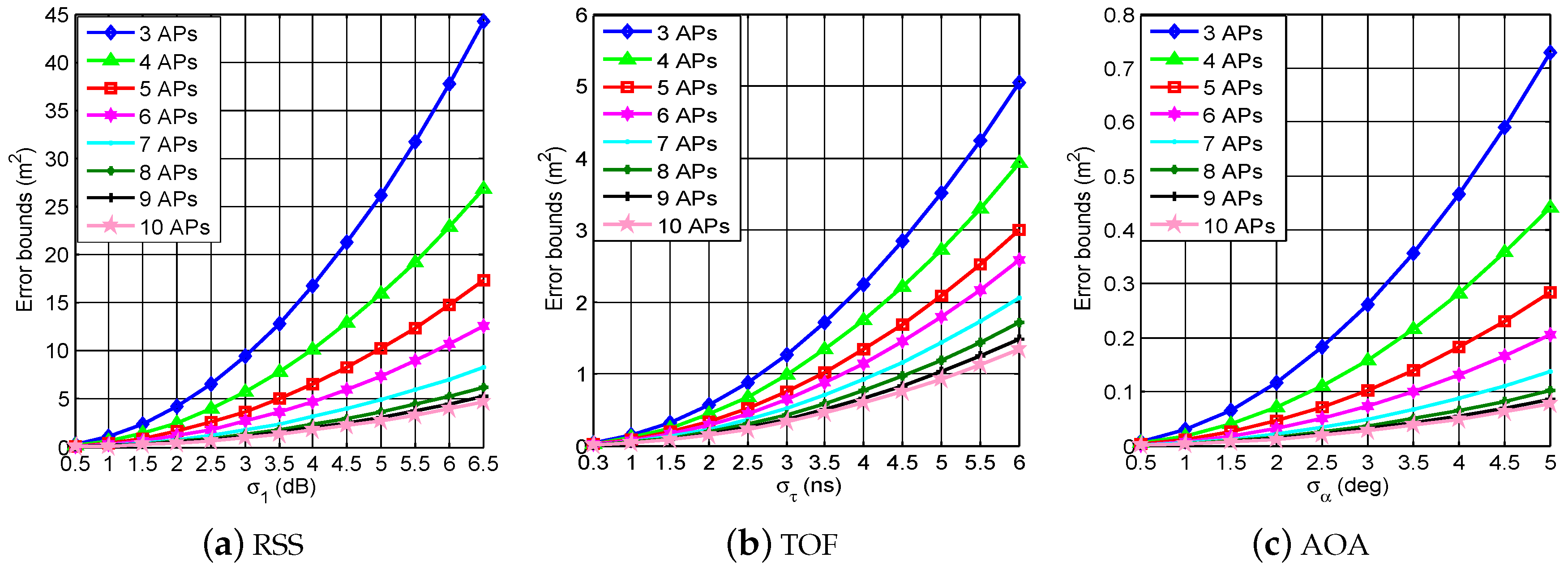
4.1. Impact of AP Number

Based on the previous discussion, we can calculate that:

$$V_m\left(\mathrm{RSS}\right)-V_{m+1}\left(\mathrm{RSS}\right)\ge \frac{{\left(\begin{array}{c}\frac{\sin {\mathsf{\alpha }}_{i(m+1)}}{d_{i(m+1)}}\sqrt{{{\eta }_{im}}_{\left(RSS\right)}{\displaystyle \sum _{k=1}^m}{\left[\frac{\cos {\mathsf{\alpha }}_{ik}}{d_{ik}}\right]}^2-{{\omega }_{im}}_{\left(RSS\right)}}\hfill \\ -\frac{\cos {\mathsf{\alpha }}_{i(m+1)}}{d_{i(m+1)}}\sqrt{{{\eta }_{im}}_{\left(RSS\right)}{\displaystyle \sum _{k=1}^m}{\left[\frac{\sin {\mathsf{\alpha }}_{ik}}{d_{ik}}\right]}^2-{{\omega }_{im}}_{\left(RSS\right)}}\hfill \end{array}\right)}^2}{{{\mathsf{\rho }}_1}^2{{\omega }_{im}}_{\left(RSS\right)}·{{\omega }_{i(m+1)}}_{\left(RSS\right)}}$$

(39)

where $\left\{\begin{array}{c}{{\eta }_{im}}_{\left(RSS\right)}={\displaystyle \sum _{k=1}^m}{\left[\frac{\cos {\mathsf{\alpha }}_{ik}}{d_{ik}}\right]}^2+{\displaystyle \sum _{k=1}^m}{\left[\frac{\sin {\mathsf{\alpha }}_{ik}}{d_{ik}}\right]}^2\hfill \\ {{\omega }_{im}}_{\left(RSS\right)}={\displaystyle \sum _{k=1}^m}{\left[\frac{\sin {\mathsf{\alpha }}_{ik}}{d_{ik}}\right]}^2\times {\displaystyle \sum _{k=1}^m}{\left[\frac{\cos {\mathsf{\alpha }}_{ik}}{d_{ik}}\right]}^2-{\left[{\displaystyle \sum _{k=1}^m}\frac{\sin {\mathsf{\alpha }}_{ik}\cos {\mathsf{\alpha }}_{ik}}{{d_{ik}}^2}\right]}^2\hfill \end{array}\right.$.

$$V_m\left(\mathrm{TOF}\right)-V_{m+1}\left(\mathrm{TOF}\right)\ge \frac{{\left(\begin{array}{c}\sin {\mathsf{\alpha }}_{i(m+1)}\sqrt{{{\eta }_{im}}_{\left(\mathrm{TOF}\right)}{\displaystyle \sum _{k=1}^m}{\left[\cos {\mathsf{\alpha }}_{ik}\right]}^2-{{\omega }_{im}}_{\left(\mathrm{TOF}\right)}}\hfill \\ -\cos {\mathsf{\alpha }}_{i(m+1)}\sqrt{{{\eta }_{im}}_{\left(\mathrm{TOF}\right)}{\displaystyle \sum _{k=1}^m}{\left[\sin {\mathsf{\alpha }}_{ik}\right]}^2-{{\omega }_{im}}_{\left(\mathrm{TOF}\right)}}\hfill \end{array}\right)}^2}{{{\mathsf{\rho }}_2}^2{{\omega }_{im}}_{\left(\mathrm{TOF}\right)}·{{\omega }_{i(m+1)}}_{\left(\mathrm{TOF}\right)}}$$

(40)

where $\left\{\begin{array}{c}{{\eta }_{im}}_{\left(\mathrm{TOF}\right)}={\displaystyle \sum _{k=1}^m}{\left[\cos {\mathsf{\alpha }}_{ik}\right]}^2+{\displaystyle \sum _{k=1}^m}{\left[\sin {\mathsf{\alpha }}_{ik}\right]}^2\hfill \\ {{\omega }_{im}}_{\left(\mathrm{TOF}\right)}={\displaystyle \sum _{k=1}^m}{\left[\sin {\mathsf{\alpha }}_{ik}\right]}^2\times {\displaystyle \sum _{k=1}^m}{\left[\cos {\mathsf{\alpha }}_{ik}\right]}^2-{\left[{\displaystyle {\displaystyle \sum _{k=1}^m}}\sin {\mathsf{\alpha }}_{ik}\cos {\mathsf{\alpha }}_{ik}\right]}^2\hfill \end{array}\right.$. ${{\eta }_{im}}_{\left(\mathrm{AOA}\right)}={{\eta }_{im}}_{\left(RSS\right)}$ and ${{\omega }_{im}}_{\left(\mathrm{AOA}\right)}={{\omega }_{im}}_{\left(\mathrm{RSS}\right)}$.

$$V_m\left(\mathrm{AOA}\right)-V_{m+1}\left(\mathrm{AOA}\right)\ge \frac{{\left(\begin{array}{c}\frac{\cos {\mathsf{\alpha }}_{i(m+1)}}{d_{i(m+1)}}\sqrt{{{\eta }_{im}}_{\left(\mathrm{AOA}\right)}{\displaystyle \sum _{k=1}^m}{\left[\frac{\sin {\mathsf{\alpha }}_{ik}}{d_{ik}}\right]}^2-{{\omega }_{im}}_{\left(\mathrm{AOA}\right)}}\hfill \\ -\frac{\sin {\mathsf{\alpha }}_{i(m+1)}}{d_{i(m+1)}}\sqrt{{{\eta }_{im}}_{\left(\mathrm{AOA}\right)}{\displaystyle \sum _{k=1}^m}{\left[\frac{\cos {\mathsf{\alpha }}_{ik}}{d_{ik}}\right]}^2-{{\omega }_{im}}_{\left(\mathrm{AOA}\right)}}\hfill \end{array}\right)}^2}{{{\mathsf{\rho }}_3}^2{{\omega }_{im}}_{\left(\mathrm{AOA}\right)}·{{\omega }_{i(m+1)}}_{\left(\mathrm{AOA}\right)}}$$

(41)

where ${{\eta }_{im}}_{\left(\mathrm{AOA}\right)}={{\eta }_{im}}_{\left(RSS\right)}$ and ${{\omega }_{im}}_{\left(\mathrm{AOA}\right)}={{\omega }_{im}}_{\left(\mathrm{RSS}\right)}$.

As can be seen from (39)–(41), the increase of AP number decreases the error bound or keeps the error bound unchanged [26]. The relation $V_m\left(m_j\right)=V_{m+1}\left(m_j\right)$ holds under the condition of ${\mathsf{\alpha }}_{i1}={\mathsf{\alpha }}_{i2}=\cdots ={\mathsf{\alpha }}_{i(m+1)}$, which indicates that the APs are collinearly distributed. Similarly, we can also find that the increase of AP number decreases the error bound or keeps the error bound unchanged by using the metric of double measurements or JMART.

4.1.1. Performance of Metric of Single Measurement

Figure 3 and Figure 4 illustrate the sum of diagonal elements in the FIM, which represents the Fisher information with respect to the metrics of RSS, TOF and AOA and the corresponding error bounds. In Figure 3, the metric of AOA is verified to be able to provide much more Fisher information compared with the metric of RSS or TOF. In addition, the larger number of APs results in the higher Fisher information as expected. Figure 4 shows that the error bound increases consistently as the variance of the metric of RSS, AOA or TOF increases. Furthermore, we also find that the smaller variance of the metric of RSS, AOA or TOF corresponds to the higher Fisher information and lower error bound in indoor localization.

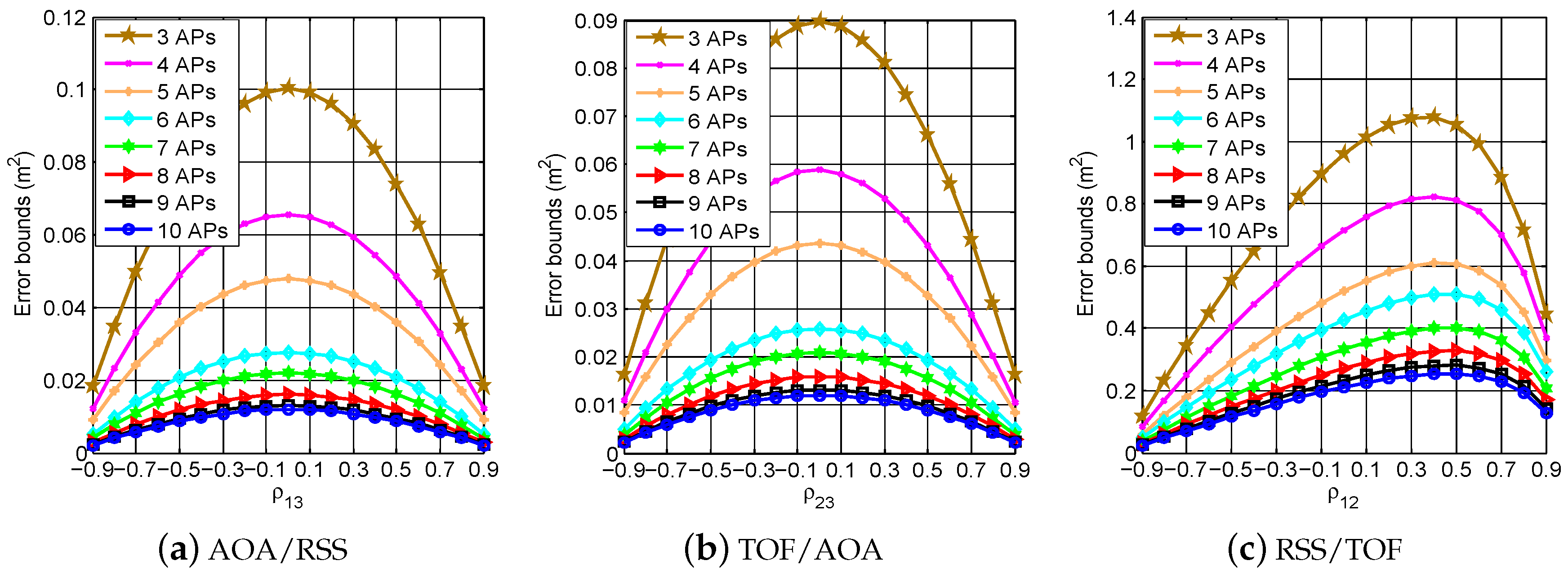
4.1.2. Performance of the Metric of Double Measurements

Figure 5 and Figure 6 illustrate the Fisher information provided by different metrics of double measurements and the corresponding error bounds. In the simulation, we set ${\mathsf{\sigma }}_1=3\mathrm{dB}$, ${\mathsf{\sigma }}_{\mathsf{\alpha }}=2.25\mathrm{deg}$ and ${\mathsf{\sigma }}_{\tau }=3\mathrm{ns}$. From these figures, the metric of TOF/AOA can be verified to perform best in providing the most Fisher information. Similarly, the larger number of APs corresponds to the higher Fisher information and lower error bound. In addition, we can find that the increase of the absolute value of correlation coefficient generally increases the Fisher information, as well as decreases the error bound.

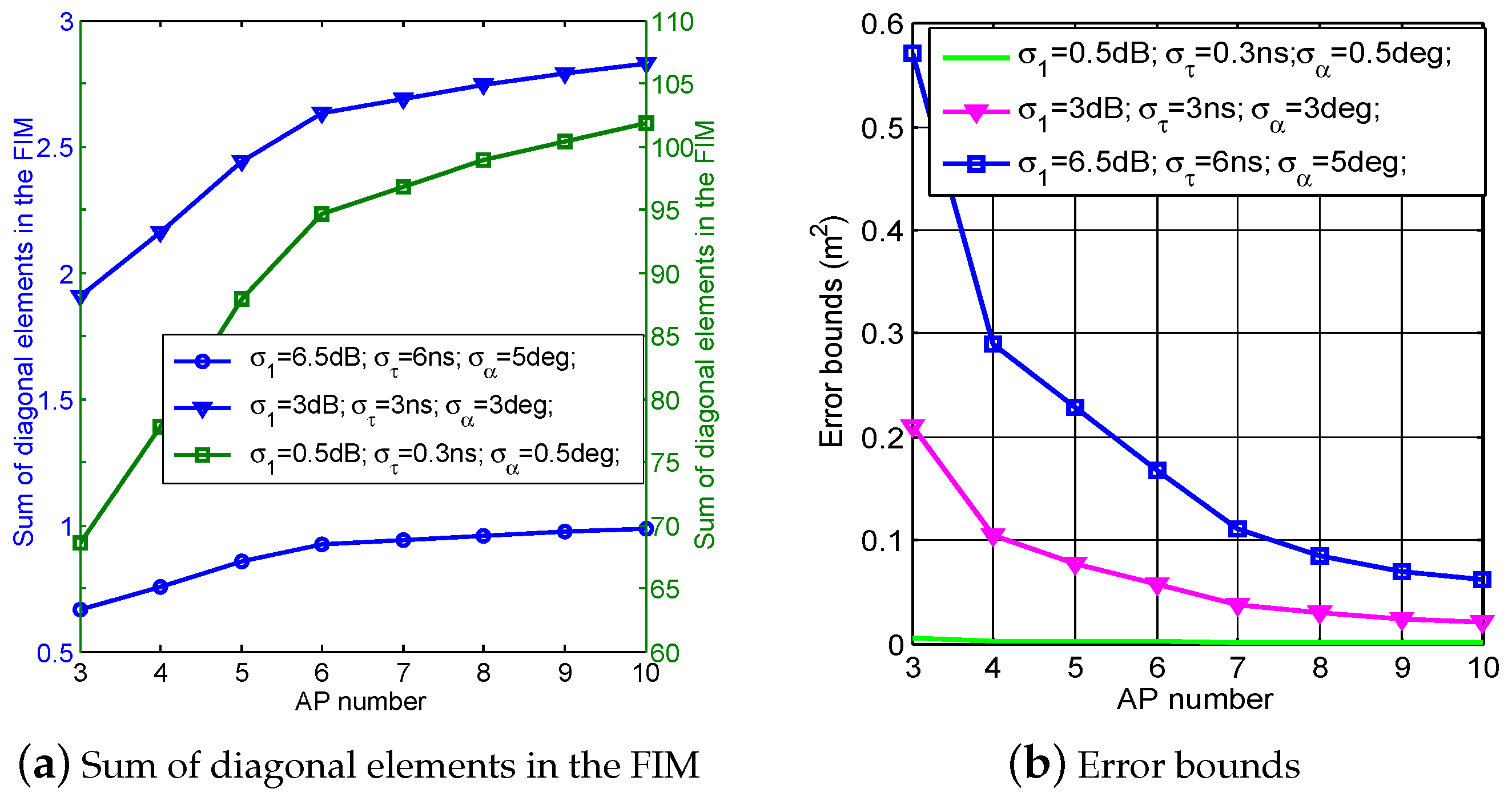
4.1.3. Performance of JMART

Figure 7 shows the Fisher information and the corresponding error bounds by the JMART. From this figure, we can find that the larger number of APs results in the higher Fisher information and lower error bounds’ indoor localization, which are in accordance with the results under the metrics of single and double measurement given above.

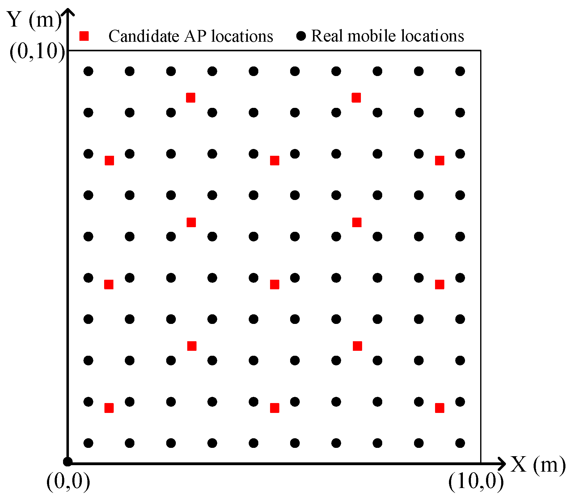
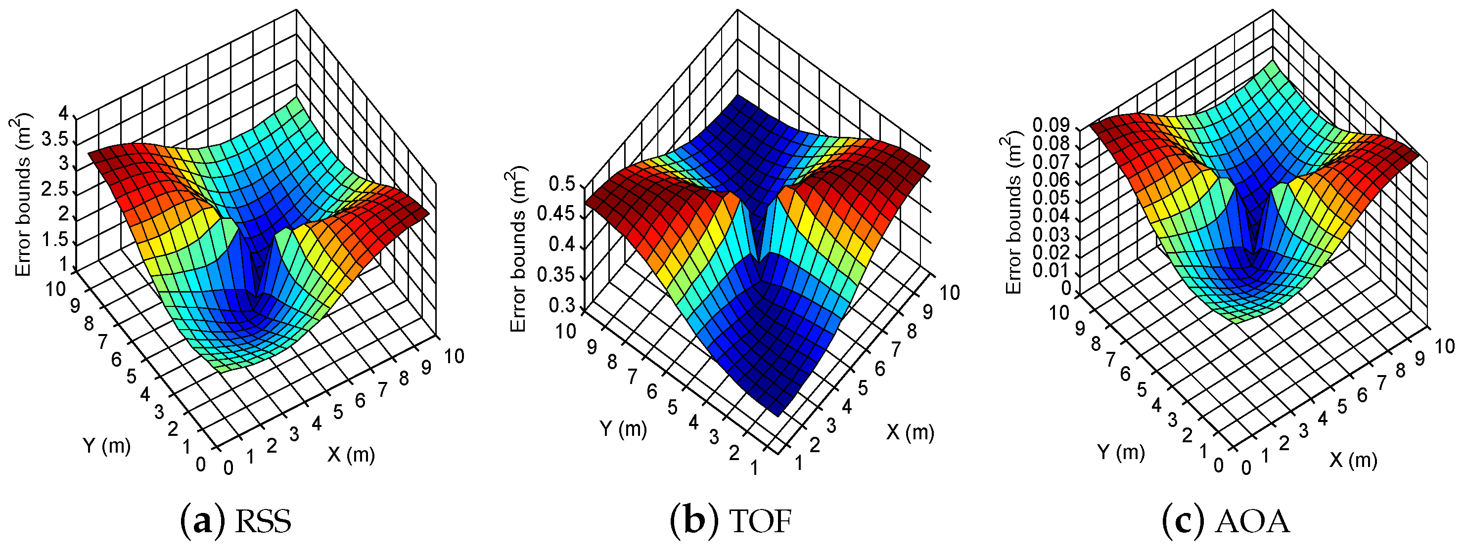
4.2. Impact of AP Locations

In this section, we will continue to investigate the relations between the error bounds and AP locations. As the distance between the i-th real location and m-th AP, $d_{im}$, decreases to ${d_{im}}^{\prime }=\ell d_{im}(0<\ell \le 1)$, we have:

$$V_m\left(\mathrm{RSS}\right)-{V_m}^{\prime }\left(\mathrm{RSS}\right)\ge \frac{{\left(\begin{array}{c}{W}_1\left(\mathrm{RSS}\right)\sqrt{{{\eta }_{i(m-1)}}_{\left(\mathrm{RSS}\right)}{\displaystyle \sum _{k=1}^{m-1}}{\left[\frac{\cos {\mathsf{\alpha }}_{ik}}{d_{ik}}\right]}^2-{\omega }_{i(m-1)\left(\mathrm{RSS}\right)}}\hfill \\ -W_2\left(\mathrm{RSS}\right)\sqrt{{{\eta }_{i(m-1)}}_{\left(\mathrm{RSS}\right)}{\displaystyle \sum _{k=1}^{m-1}}{\left[\frac{\sin {\mathsf{\alpha }}_{ik}}{d_{ik}}\right]}^2-{\omega }_{i(m-1)\left(\mathrm{RSS}\right)}}\hfill \end{array}\right)}^2}{{{\mathsf{\rho }}_1}^2·{{\omega }_{im}}_{\left(\mathrm{RSS}\right)}·{{{\omega }^{\prime }}_{im}}_{\left(\mathrm{RSS}\right)}}$$

(42)

where $\left\{\begin{array}{c}{\cos }^{\prime }{\mathsf{\alpha }}_{im}=\frac{x_i-{x_m}^{\prime }}{\ell d_{im}};{\sin }^{\prime }{\mathsf{\alpha }}_{im}=\frac{y_i-{y_m}^{\prime }}{\ell d_{im}}\hfill \\ W_1\left(\mathrm{RSS}\right)=\frac{{\left({\sin }^{\prime }{\mathsf{\alpha }}_{\mathrm{im}}\right)}^2}{{\ell }^2{{\mathrm{d}}_{\mathrm{im}}}^2}-\frac{{\sin }^2{\mathsf{\alpha }}_{\mathrm{im}}}{{{\mathrm{d}}_{\mathrm{im}}}^2}\hfill \\ W_2\left(\mathrm{RSS}\right)=\frac{{\left({\cos }^{\prime }{\mathsf{\alpha }}_{\mathrm{im}}\right)}^2}{{\ell }^2{{\mathrm{d}}_{\mathrm{im}}}^2}-\frac{{\cos }^2{\mathsf{\alpha }}_{\mathrm{im}}}{{{\mathrm{d}}_{\mathrm{im}}}^2}\hfill \end{array}\right.$ and ${{\omega }^{\prime }}_{im\left(\mathrm{RSS}\right)}={\displaystyle \sum _{k=1}^{m-1}}\left(\frac{{\sin }^2{\mathsf{\alpha }}_{ik}}{{d_{ik}}^2}+\frac{{{\sin }^{\prime }}^2{\mathsf{\alpha }}_{im}}{{\ell }^2{d_{im}}^2}\right){\displaystyle \sum _{k=1}^{m-1}}\left(\frac{{\cos }^2{\mathsf{\alpha }}_{ik}}{{d_{ik}}^2}+\frac{{{\cos }^{\prime }}^2{\mathsf{\alpha }}_{im}}{{\ell }^2{d_{im}}^2}\right)$ $-{\left[{\displaystyle \sum _{k=1}^{m-1}}\frac{\sin {\mathsf{\alpha }}_{ik}\cos {\mathsf{\alpha }}_{ik}}{{d_{ik}}^2}+\frac{{\sin }^{\prime }{\mathsf{\alpha }}_{im}{\sin }^{\prime }{\mathsf{\alpha }}_{im}}{{\ell }^2{d_{im}}^2}\right]}^2$.

$$V_m\left(\mathrm{TOF}\right)-{V_m}^{\prime }\left(\mathrm{TOF}\right)\ge \frac{{\left(\begin{array}{c}{W}_1\left(\mathrm{TOF}\right)\sqrt{{{\eta }_{i(m-1)}}_{\left(\mathrm{TOF}\right)}{\displaystyle \sum _{k=1}^{m-1}}{\left[\cos {\mathsf{\alpha }}_{ik}\right]}^2-{\omega }_{i(m-1)\left(\mathrm{TOF}\right)}}\hfill \\ -W_2\left(\mathrm{TOF}\right)\sqrt{{{\eta }_{i(m-1)}}_{\left(\mathrm{TOF}\right)}{\displaystyle \sum _{k=1}^{m-1}}{\left[\sin {\mathsf{\alpha }}_{ik}\right]}^2-{\omega }_{i(m-1)\left(\mathrm{TOF}\right)}}\hfill \end{array}\right)}^2}{{{\mathsf{\rho }}_2}^2·{{\omega }_{im}}_{\left(\mathrm{TOF}\right)}·{{{\omega }^{\prime }}_{im}}_{\left(\mathrm{TOF}\right)}}$$

(43)

where $\left\{\begin{array}{c}{W}_1\left(\mathrm{TOF}\right)={\left({\sin }^{\prime }{\mathsf{\alpha }}_{im}\right)}^2-{\left(\sin {\mathsf{\alpha }}_{im}\right)}^2\hfill \\ W_2\left(\mathrm{TOF}\right)={\left({\cos }^{\prime }{\mathsf{\alpha }}_{im}\right)}^2-{\left(\cos {\mathsf{\alpha }}_{im}\right)}^2\hfill \end{array}\right.$, ${{\omega }^{\prime }}_{im\left(\mathrm{TOF}\right)}={\displaystyle \sum _{k=1}^{m-1}}\left({\sin }^2{\mathsf{\alpha }}_{ik}+{{\sin }^{\prime }}^2{\mathsf{\alpha }}_{im}\right){\displaystyle \sum _{k=1}^{m-1}}\left({\cos }^2{\mathsf{\alpha }}_{ik}+{{\cos }^{\prime }}^2{\mathsf{\alpha }}_{im}\right)$$-{\left[{\displaystyle \sum _{k=1}^{m-1}}\sin {\mathsf{\alpha }}_{ik}\cos {\mathsf{\alpha }}_{ik}+{\sin }^{\prime }{\mathsf{\alpha }}_{im}{\sin }^{\prime }{\mathsf{\alpha }}_{im}\right]}^2$ .

$$V_m\left(\mathrm{AOA}\right)-{V_m}^{\prime }\left(\mathrm{AOA}\right)\ge \frac{{\left(\begin{array}{c}{W}_2\left(\mathrm{AOA}\right)\sqrt{{{\eta }_{i(m-1)}}_{\left(\mathrm{AOA}\right)}{\displaystyle \sum _{k=1}^{m-1}}\frac{{\sin }^2{\mathsf{\alpha }}_{ik}}{{d_{ik}}^2}-{\omega }_{i(m-1)\left(\mathrm{AOA}\right)}}\hfill \\ -W_1\left(\mathrm{AOA}\right)\sqrt{{{\eta }_{i(m-1)}}_{\left(\mathrm{AOA}\right)}{\displaystyle \sum _{k=1}^{m-1}}\frac{{\cos }^2{\mathsf{\alpha }}_{ik}}{{d_{ik}}^2}-{\omega }_{i(m-1)\left(\mathrm{AOA}\right)}}\hfill \end{array}\right)}^2}{{{\mathsf{\rho }}_3}^2·{{\omega }_{im}}_{\left(\mathrm{AOA}\right)}·{{{\omega }^{\prime }}_{im}}_{\left(\mathrm{AOA}\right)}}$$

(44)

where ${{\omega }^{\prime }}_{im\left(\mathrm{AOA}\right)}={{\omega }^{\prime }}_{im\left(\mathrm{RSS}\right)}$. Similarly, we can also find that the decrease of the distance between the i-th real location and k-th AP decreases the error bound or keeps the error bound unchanged by using the metric of double measurements or JMART. To show this result more clearly, we conduct the simulations in a square area with the dimensions of 10 m by 10 m, as shown in Figure 2. By fixing three APs at the locations (10 m, 10 m), (10 m, 0 m) and (0 m, 10 m), we calculate the error bounds with respect to the mobile location (5 m, 5 m) as a function of the fourth AP $\in \left[0,10\mathrm{m}\right]\times \left[0,10\mathrm{m}\right]$ in Figure 8, Figure 9 and Figure 10.

4.2.1. Performance of the Metric of Single Measurement

From Figure 8, we can find that the smaller distance between the i-th real location and fourth AP generally results in the lower error bound. Based on this, we can optimize the AP locations towards the lowest error bounds.

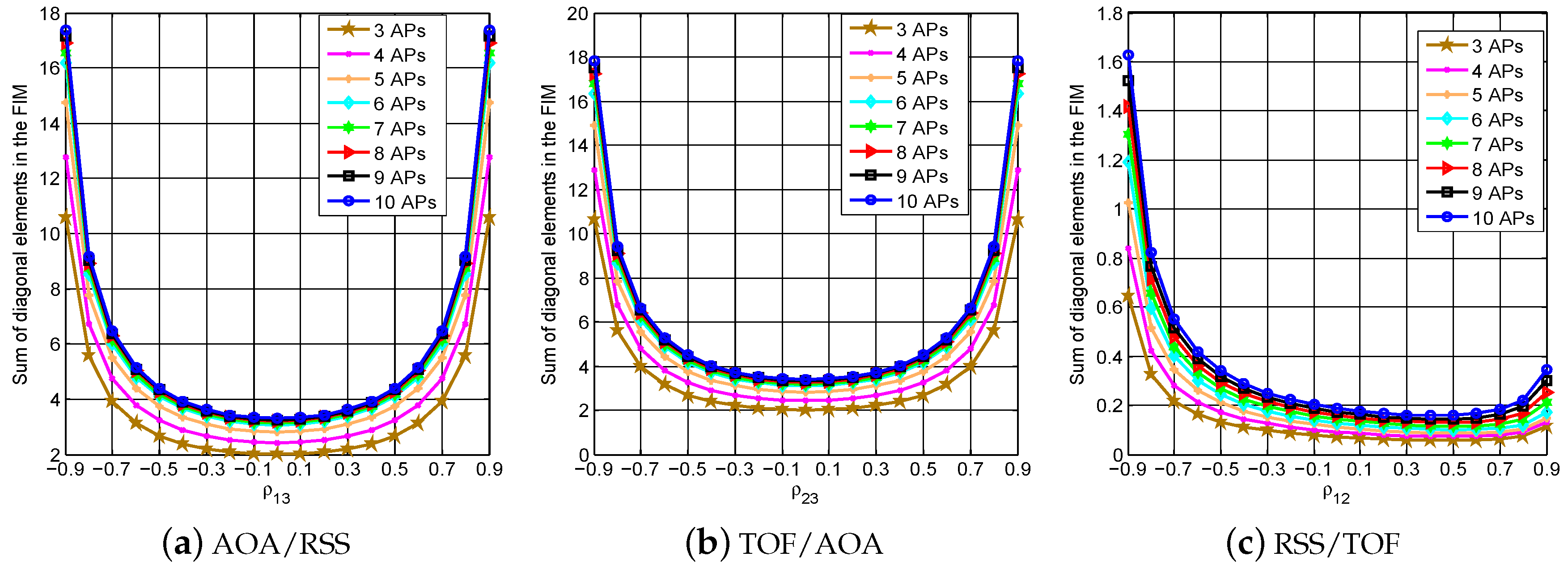
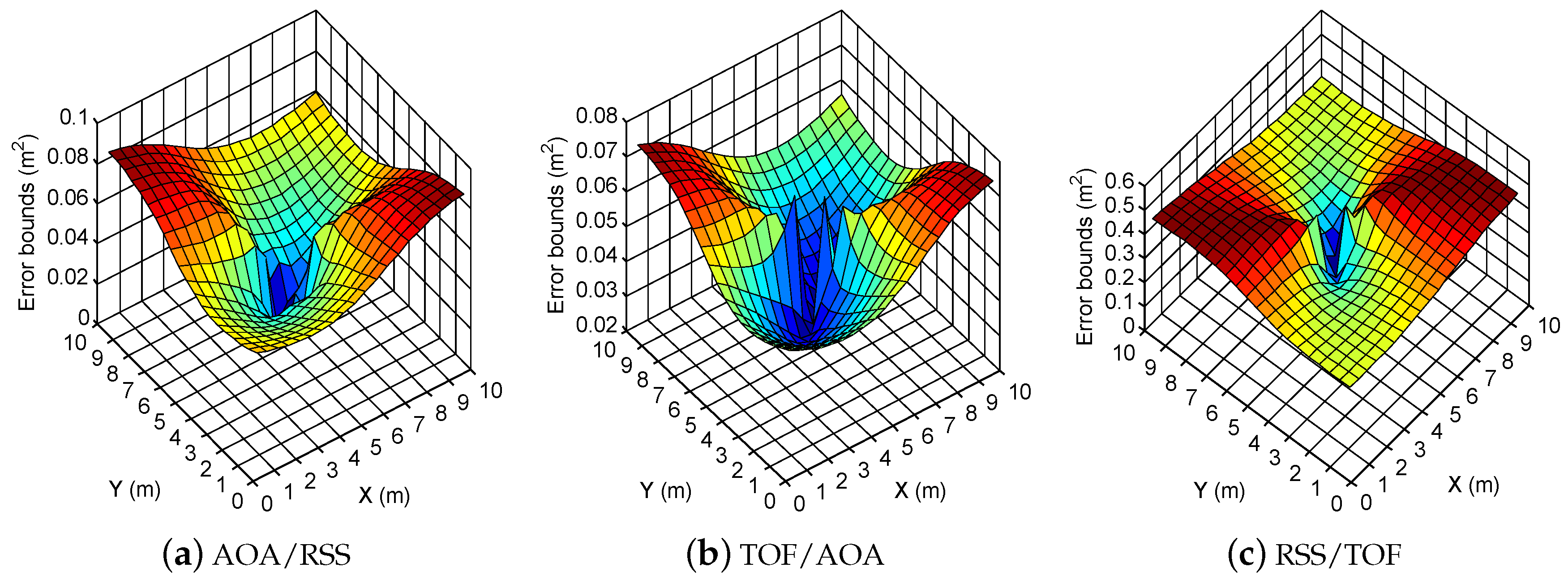
4.2.2. Performance of Metric of Double Measurements

Figure 9 shows the error bounds by using different metrics of double measurements. The relations between the error bounds and AP locations exhibited in Figure 9 are in accordance with the ones by using the metric of a single measurement. In addition, based on the results in Figure 9 and Figure 10, the error bounds achieved by the metric of double measurements are lower than the ones by the metric of single measurement.

4.2.3. Performance of JMART

Figure 10 shows the error bounds under different locations of the fourth AP by using the JMART for localization. Obviously, the error bounds achieved by the JMART are the lowest compared with the ones by the metrics of single and double measurements.

4.3. Impact of Noise Power

Based on the previous discussion in Section 3, the deviation of the metrics of RSS, AOA and TOF (or called noise power) determines the values of ${\mathsf{\rho }}_1$, ${\mathsf{\rho }}_2$ and ${\mathsf{\rho }}_3$ and thereby affects the error bound. Then, in this section, we will focus on the impact of the deviation of the metrics of RSS, AOA and TOF on error bounds.

4.3.1. Performance of Metric of Single Measurement

In Figure 3 and Figure 4, we have illustrated the relations between the error bounds and the deviation of the metrics of RSS, AOA and TOF [27]. The increase of the deviation of the metrics of RSS, AOA and TOF consistently decreases the Fisher information and meanwhile increases the error bounds.

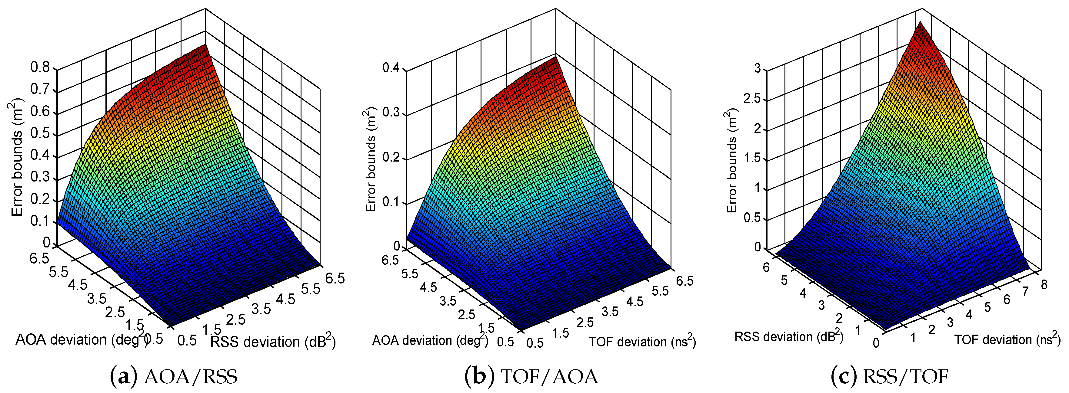
4.3.2. Performance of Metric of Double Measurements

Figure 11 and Figure 12 show the Fisher information provided by using the metrics of AOA/RSS, TOF/AOA and RSS/TOF and the corresponding error bounds under different deviations of the metrics of RSS, AOA and TOF. From these figures, we can find that the Fisher information and error bounds are highly affected by AOA deviation, while the impact of RSS and TOF deviation on the Fisher information and error bounds is slight.

4.3.3. Performance of JMART

Finally, Figure 13 shows the variation of the Fisher information and the corresponding error bounds by the JMART under different deviations of the metrics of RSS, AOA and TOF. From this figure, we can find that both the Fisher information and error bounds are significantly determined by AOA deviation, which are in accordance with the results under the metrics of single and double measurement given above.

5. Conclusions

In this paper, we present the theoretical analysis of the error bounds by selecting the single, double and JMART measurements as the metric for indoor localization. The purpose of the analysis is to better design an indoor localization system, either through the judicious selection of the metrics for localization or though the optimal AP deployment. Based on the extensive simulations, we find that the JMART is able to provide higher Fisher information, as well as achieve lower error bounds compared with the ones by using the metrics of single and double measurements. Furthermore, we find that the increase of AP number decreases the error bounds or keeps the error bounds unchanged, while as the noise power increases, the error bounds with respect to the single, double and JMART measurements will also increase. In general, since the smaller distance between the AP and testing locations results in the lower error bound, we are able to optimize the AP locations towards the lowest error bound. Our future work is to rely on the analytical relations of the Fisher information, error bounds, metrics used for localization and AP deployment to design a more effective indoor localization system, and meanwhile, we will continue to study the error bounds for the biased localization problem by using different metrics for the indoor localization.

References

1. Barrios, C.; Motai, Y. Improving Estimation of Vehicle’s Trajectory Using the Latest Global Positioning System With Kalman Filtering. IEEE Trans. Instrum. Meas. 2011, 60, 3747–3755. [Google Scholar] [CrossRef]
2. Zhou, M.; Wong, A.K.; Tian, Z.; Luo, X.; Xu, K.; Shi, R. Personal mobility map construction for crowd-sourced Wi-Fi based indoor mapping. IEEE Commun. Lett. 2014, 18, 1427–1430. [Google Scholar] [CrossRef]
3. Kim, Y.; Shin, H.; Chon, Y.; Cha, H.; Campos, M. Crowdsensing-based Wi-Fi radio map management using a lightweight site survey. Comput. Commun. 2015, 60, 86–96. [Google Scholar] [CrossRef]
4. Zhou, M.; Zhang, Q.; Xu, K.; Tian, Z.; Meng, Y.; He, W. PRIMAL: Page rank based indoor mapping and localization using gene sequenced unlabeled WLAN received signal strength. Sensors 2015, 15, 24791–24817. [Google Scholar] [CrossRef] [PubMed]
5. Hossain, A.K.M.M.; Soh, W.S. A survey of calibration-free indoor positioning systems. Comput. Commun. 2015, 66, 1–13. [Google Scholar] [CrossRef]
6. Kaemarungsi, K.; Krishnamurthy, P. Properties of indoor received signal strength for WLAN location fingerprinting. In Proceedings of the 1st Annual International Conference on Mobile and Ubiquitous Systems: Networking and Services, Boston, MA, USA, 26 August 2004; pp. 14–23.
7. Gustafsson, F.; Gunnarsson, F. Mobile positioning using wireless networks: Possibilities and fundamental limitations based on available wireless network measurements. IEEE Signal Process. Mag. 2005, 22, 41–53. [Google Scholar] [CrossRef]
8. Prince, G.B.; Little, T.D.C. A two phase hybrid RSS/AoA algorithm for indoor device localization using visible light. In Proceedings of the IEEE GLOBECOM, Anaheim, CA, USA, 3–7 December 2012; pp. 3347–3352.
9. Kim, R.; Lim, H.; Hwang, S.N.; Obele, B.O. Robust indoor localization based on hybrid Bayesian graphical models. In Proceedings of the IEEE GLOBECOM, Austin, TX, USA, 8–12 December 2014; pp. 423–429.
10. Yu, K.; Guo, Y.J. Statistical NLOS Identification Based on AOA, TOA, and Signal Strength. IEEE Trans. Veh. Technol. 2009, 58, 274–286. [Google Scholar] [CrossRef]
11. Tomic, S.; Beko, M.; Dinis, R. Distributed RSS-AoA Based Localization With Unknown Transmit Powers. IEEE Wirel. Commun. Lett. 2016, 5, 392–395. [Google Scholar] [CrossRef]
12. Wang, H.; Yip, L.; Yao, K.; Estrin, D. Lower bounds of localization uncertainty in sensor networks. In Proceedings of the IEEE International Conference on Acoustics, Speech, and Signal Processing, Montreal, QC, Canada, 17–21 May 2004; pp. 16–18.
13. Zheng, X.; liu, H.; Yang, J.; Chen, Y. A Study of Localization Accuracy Using Multiple Frequencies and Powers. IEEE Trans. Parallel Distrib. Syst. 2014, 25, 1955–1965. [Google Scholar] [CrossRef]
14. Yan, K.; Wu, H.C.; Lyengar, S.S. Robustness analysis and new hybrid algorithm of wideband source localization for acoustic sensor networks. IEEE Trans. Wirel. Commun. 2010, 9, 2033–2043. [Google Scholar] [CrossRef]
15. Nguyen, T.V.; Jeong, Y.; Shin, H.; Win, M.Z. Least Square Cooperative Localization. IEEE Trans. Veh. Technol. 2015, 64, 1318–1330. [Google Scholar] [CrossRef]
16. Wei, Q.; Zhang, D.; Han, J. Improved localisation method based on multi-hop distance unbiased estimation. IET Commun. 2014, 8, 2797–2804. [Google Scholar] [CrossRef]
17. Angjelichinoski, M.; Denkovski, D.; Atanasovski, V.; Gavrilovska, L. Cramer-Rao lower bounds of RSS-based localization with anchor position uncertainty. IEEE Trans. Inf. Theory 2015, 61, 2807–2834. [Google Scholar] [CrossRef]
18. Gazzah, L.; Najjar, L.; Besbes, H. Improved selective hybrid RSS/AOA weighting schemes for NLOS localization. In Proceedings of the 2014 International Conference on Multimedia Computing and Systems, Marrakech, Morocco, 14–16 April 2014; pp. 746–751.
19. Prieto, J.; Mazuelas, S.; Bahillo, A.; Fernandez, P. Adaptive data fusion for wireless localization in harsh environments. IEEE Trans. Signal Process. 2012, 60, 1585–1596. [Google Scholar] [CrossRef]
20. Wang, S.C.; Jackson, B.R.; Inkol, R. Hybrid RSS/AOA emitter location estimation based on least squares and maximum likelihood criteria. In Proceedings of the IEEE Biennial Symposium on Communications, Kingston, ON, Canada, 28–29 May 2012; pp. 24–29.
21. Chan, F.; Wen, C. Adaptive AOA/TOA Localization Using Fuzzy Particle Filter for Mobile WSNs. In Proceedings of the IEEE VTC, Budapest, Hungary, 15–18 May 2011; pp. 1–5.
22. Venkatesh, S.; Buehrer, M. Multiple-access insights from bounds on sensor localization. In Proceedings of the World of Wireless, Mobile and Multimedia Networks, Buffalo, NY, USA, 26–29 June 2006; pp. 2–12.
23. Shen, Y.; Wymeersch, H.; Win, M.Z. Fundamental limits of wideband cooperative localization via fisher information. In Proceedings of the Wireless Communications and Networking Conference, Hong Kong, China, 11–15 March 2007; pp. 3954–3958.
24. Dersan, A.; Tanik, Y. Passive radar localization by time difference of arrival. In Proceedings of the IEEE MILCOM, Anaheim, CA, USA, 7–10 October 2002; pp. 1251–1257.
25. Chang, C.; Sahai, A. Estimation bounds for localization. In Proceedings of the IEEE Sensor and Ad Hoc Communications and Networks, Santa Clara, CA, USA, 4–7 October 2004; pp. 415–424.
26. Hossain, A.K.M.M.; Soh, W.S. Cramer-Rao Bound Analysis of Localization Using Signal Strength Difference as Location Fingerprint. In Proceedings of the IEEE INFOCOM, San Diego, CA, USA, 14–19 March 2010; pp. 1–9.
27. Patwari, N.; Hero, A.O. Location estimation accuracy in wireless sensor networks. In Proceedings of the IEEE Asilomar Conference on Signals, Systems and Computers, Pacific Grove, CA, USA, 3–6 November 2002; pp. 1523–1527.
28. Qi, Y.; Suda, H.; Kobayashi, H. On time-of-arrival positioning in a multipath environment. In Proceedings of the IEEE VTC, Milan, Italy, 17–19 May 2004; pp. 3540–3544.
29. Botteron, C.; Host-Madsen, A.; Fattouche, M. Effects of system and environment parameters on the performance of network-based mobile station position estimators. IEEE Trans. Veh. Technol. 2004, 53, 163–180. [Google Scholar] [CrossRef]
30. Botteron, C.; Host-Madsen, A.; Fattouche, M. Cramer-Rao bounds for the estimation of multipath parameters and mobiles’ positions in asynchronous DS-CDMA systems. IEEE Trans. Signal Process. 2004, 52, 862–875. [Google Scholar] [CrossRef]
31. Trees, H.L.V. Optimum Array Processing: Part IV of Detection, Estimation and Modulation Theory; John Wiley & Sons, Inc.: Hoboken, NJ, USA, 2002. [Google Scholar]
32. Alasti, H.; Xu, K.; Dang, Z. Efficient experimental path loss exponent measurement for uniformly attenuated indoor radio channels. In Proceedings of the IEEE Southeastcon, Atlanta, GA, USA, 5–8 March 2009; pp. 255–260.
33. Herring, T.; Holloway, W.; Staelin, H. Path-Loss Characteristics of Urban Wireless Channels. IEEE Trans. Antennas Propag. 2010, 58, 171–177. [Google Scholar] [CrossRef]
34. Eisayed, H.; Athanasious, G.; Fischione, C. Evaluation of localization methods in millimeter-wave wireless systems. In Proceedings of the IEEE Computer Aided Modeling and Design of Communication Links and Networks, Athens, Greece, 1–3 December 2014; pp. 345–349.
Figure 1. Geometric relations between the i-th real location and k-th Access Point (AP).
Applsci 06 00296 g001
Figure 2. Layout of candidate mobile and AP locations.
Applsci 06 00296 g002
Figure 3. Sum of diagonal elements in the Fisher Information Matrix (FIM) with respect to the metrics of (a) Signal Strength (RSS), (b) Time-of-flight (TOF) and (c) Angle-of-arrival (AOA).
Applsci 06 00296 g003
Figure 4. Error bounds achieved by the metrics of Receive (a) RSS, (b) TOF and (c) AOA.
Applsci 06 00296 g004
Figure 5. Sum of diagonal elements in the FIM with respect to the metrics of (a) AOA/RSS, (b) TOF/AOA and (c) RSS/TOF.
Applsci 06 00296 g005
Figure 6. Error bounds achieved by the metrics of (a) AOA/RSS, (b) TOF/AOA and (c) RSS/TOF.
Applsci 06 00296 g006
Figure 7. Sum of diagonal elements in the (a) FIM and (b) error bounds by the Joint Metric of AOA/RSS/TOF (JMART).
Applsci 06 00296 g007
Figure 8. Error bounds under different locations of the fourth AP by the metrics of (a) RSS, (b) TOF and (c) AOA.
Applsci 06 00296 g008
Figure 9. Error bounds under different locations of the fourth AP by the metrics of (a) AOA/RSS, (b) TOF/AOA and (c) RSS/TOF.
Applsci 06 00296 g009
Figure 10. Error bounds under different locations of the fourth AP by the JMART.
Applsci 06 00296 g010
Figure 11. Sum of the diagonal elements in the FIM by using the hybrid (a) AOA/RSS, (b) TOF/AOA and (c) RSS/TOF.
Applsci 06 00296 g011
Figure 12. Error bounds by using the hybrid (a) AOA/RSS, (b) TOF/AOA and (c) RSS/TOF.
Applsci 06 00296 g012
Figure 13. Sum of diagonal elements in the FIM (a) and error bounds (b) by the JMART.
Applsci 06 00296 g013