
Passive Guaranteed Simulation of Analog Audio Circuits: A Port-Hamiltonian Approach


Abstract
:1. Introduction
- Analog circuits combine energy-storing components, dissipative components, and sources.
- Storage components do not produce energy, and dissipative components decrease it.
2. Port-Hamiltonian Systems
2.1. Formalism and Property
2.1.1. Components
- internal components that store energy (capacitors or inductors),
- internal components that dissipate power (resistors, diodes, transistors, etc.),
- external ports that convey power from sources (voltage or current generators) or any external system (active, dissipative, or mixed).
2.1.2. Conservative Interconnection
- expresses the conservative power exchanges between storage components (this corresponds to the so-called matrix in classical Hamiltonian systems);
- expresses the conservative power exchanges between dissipative components;
- expresses the conservative power exchanges between ports (direct connections of inputs to outputs);
- expresses the conservative power exchanges between the storage components and the dissipative components;
- expresses the conservative power exchanges between ports and storage components (input gain matrix);
- expresses the conservative power exchanges between ports and dissipative components (input gain matrix).
2.2. Example
3. Generation of Equations
- Step 1:
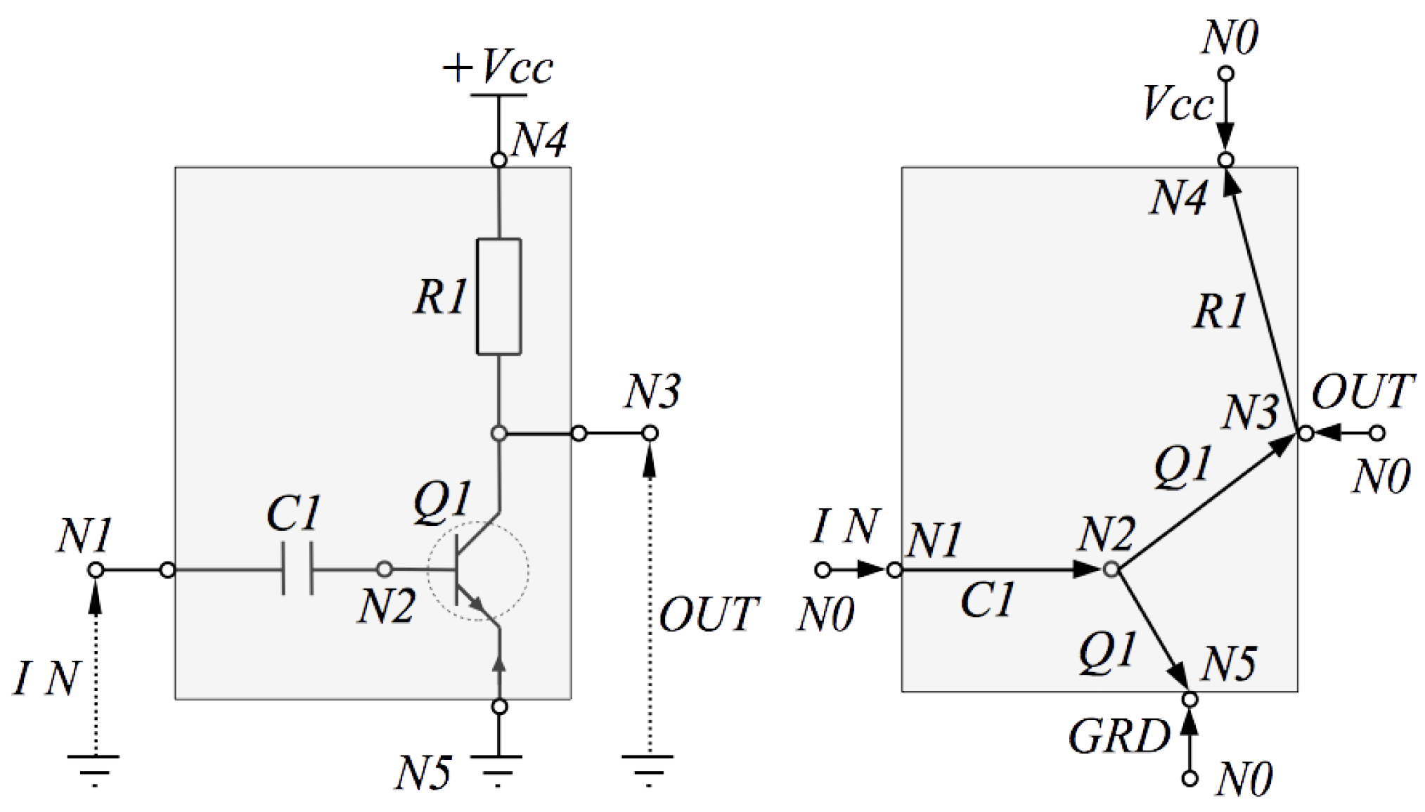
- from a netlist () to a graph () that represents the Kirchhoff’s laws for a chosen orientation (convention);
- Step 2:
- from () to the skew-symmetric matrix in (5).
3.1. Graph Encoding
3.1.1. Netlists
3.1.2. Graph
- Dipoles are made of two nodes and a single branch, defining a single couple of state x and storage function (storage component), or dissipative variable w and scalar relation (dissipative components).
- More generally, n-ports multipole are made of n nodes and at least branches, defining couples of variables and functions. Typically, the graph for the bipolar junction is made of two branches (base-emitter and base-collector).
- build the internal graph by connecting the elementary graph of the components from the first block of the netlist,
- introduce a reference node (or datum, see [27] §10) to define the external branches from the second block.
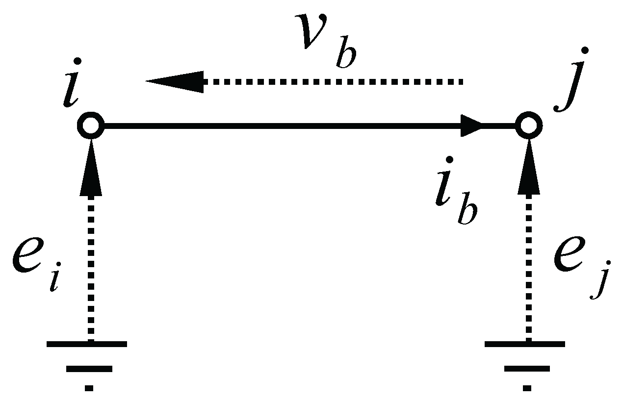
3.1.3. Kirchhoff’s Laws on Graphs

3.2. Realizability Analysis
3.2.1. A Criterion for Realizability
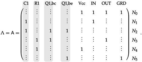
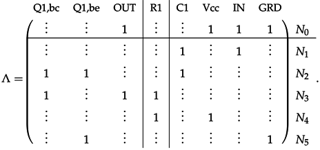
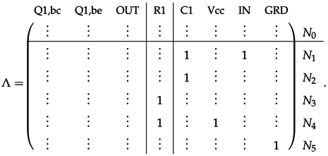
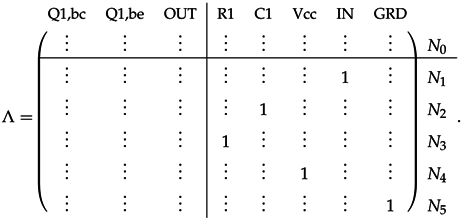
3.2.2. Algorithm
- (C1)
- The potential on each node is uniquely defined so that .
- (C2)
- Each Current-controlled edge propagates the knowledge of the potential on one node to the other, so that .
- (C3)
- No edge imposes the reference potential so that .
- (C4)
- No voltage-controlled edge imposes any potential so that .
| Algorithm 1: Analysis of realizability. If successfully complete, the resulting PHS structure is given by the procedure in the proof of Proposition 1 |
 |
3.2.3. Example
4. Guaranteed-Passive Simulation
4.1. Numerical Scheme
4.2. Solving the Implicit Equations
| Algorithm 2: Simulation, with the number of time-steps and the (fixed) number of Newton–Raphson iterations. |
 |
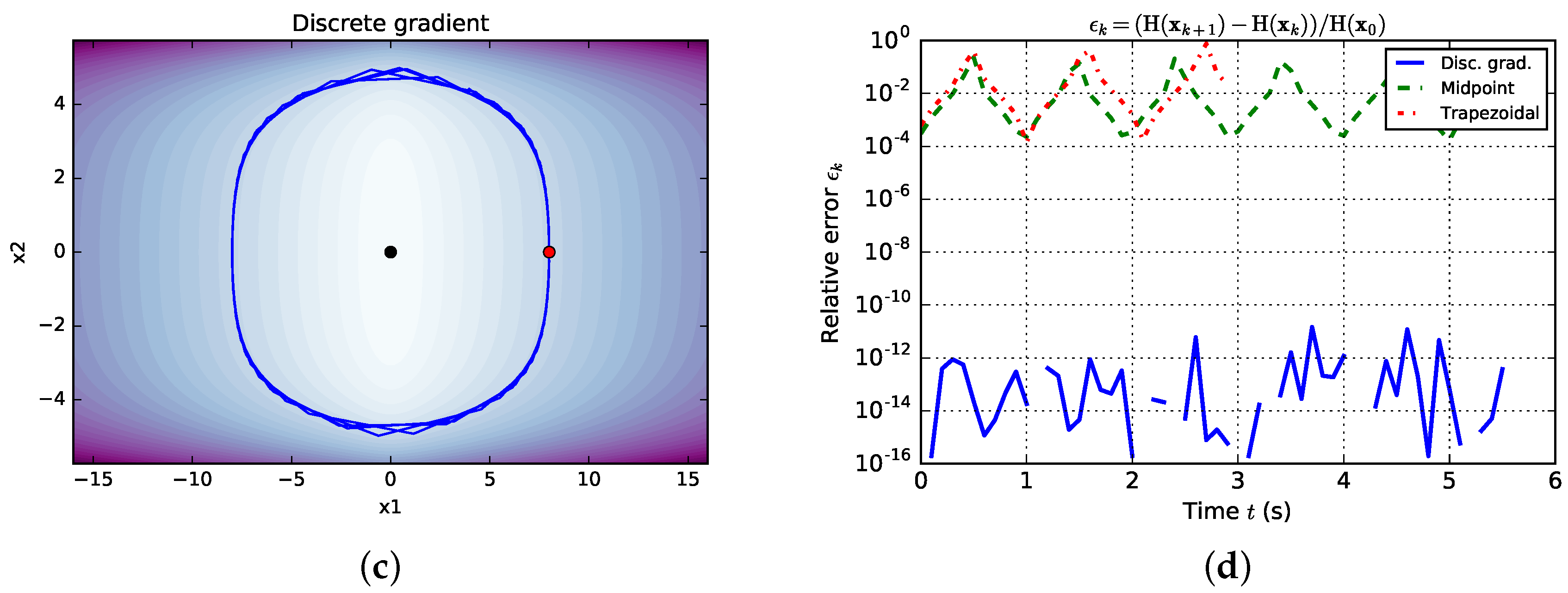
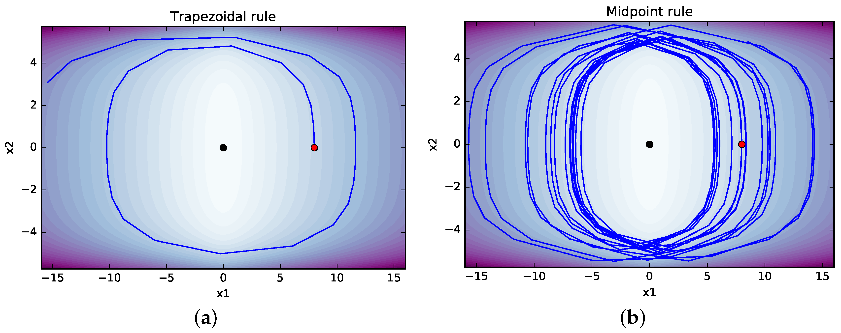
4.3. Comparison with Standard Methods
5. Applications
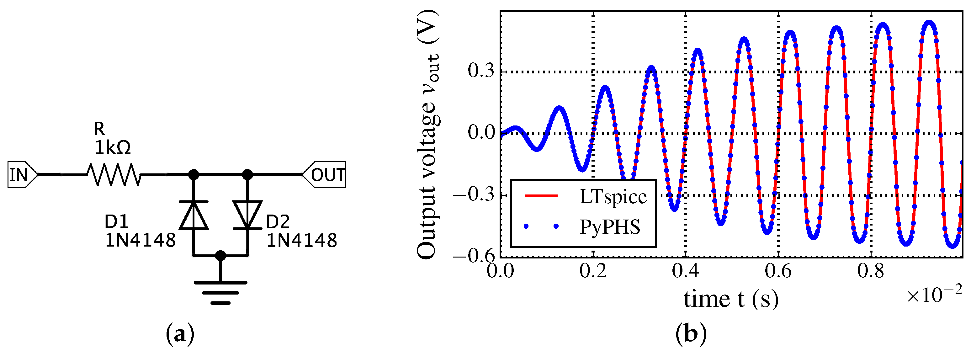
5.1. Diode Clipper
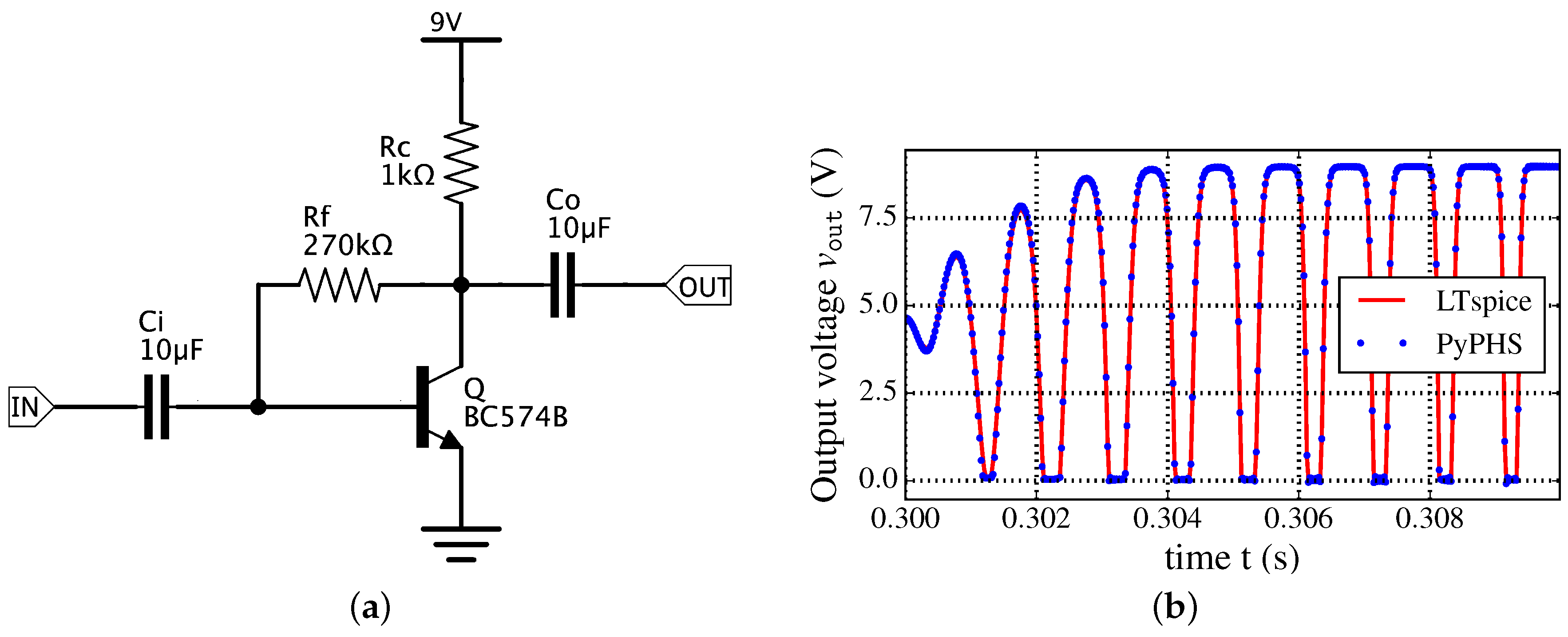
5.2. Common-Emitter BJT Audio Amplifier
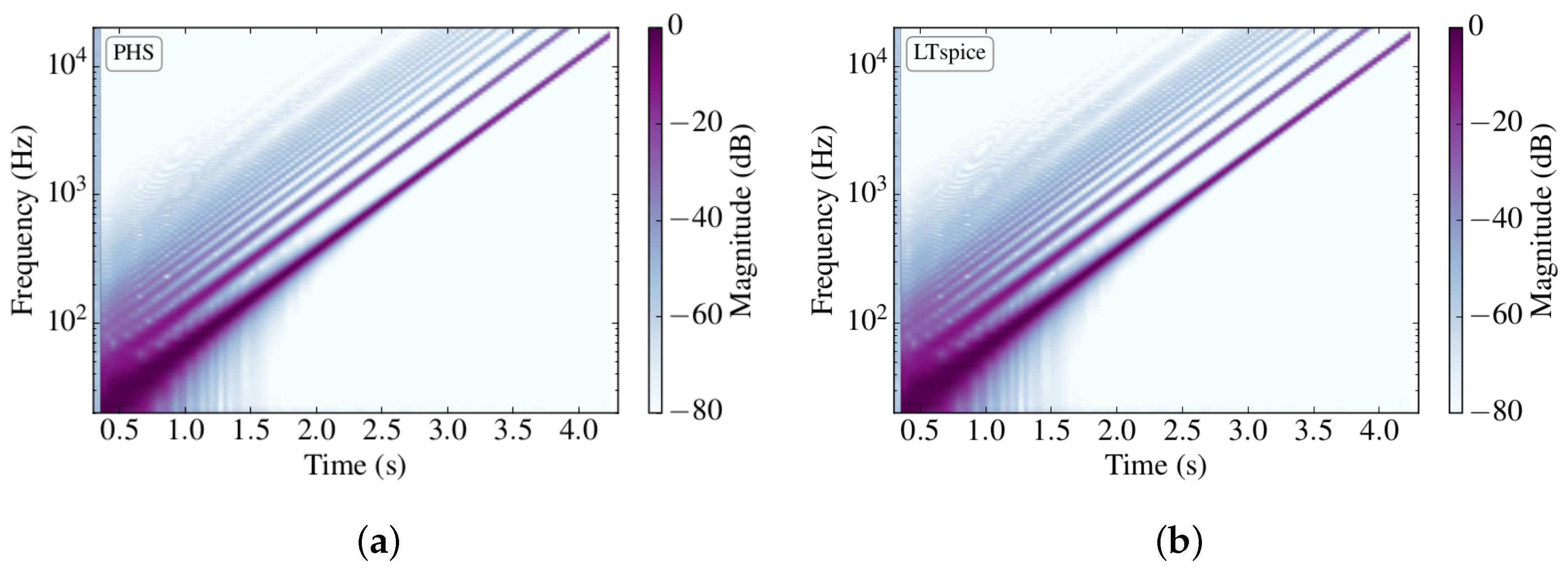
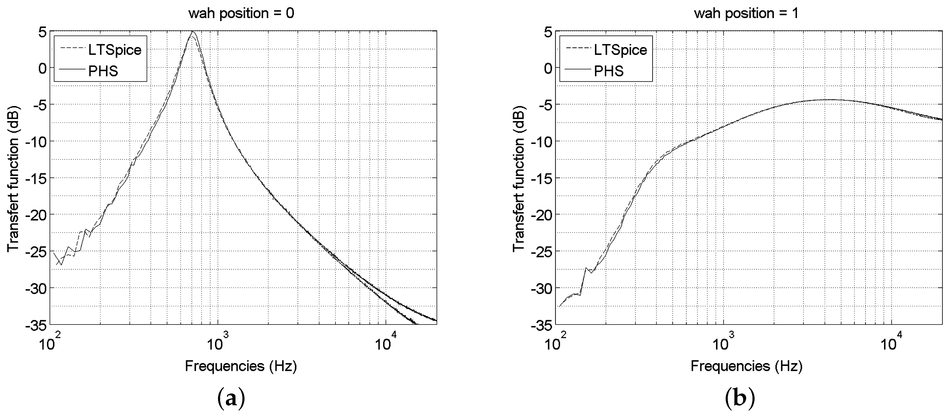
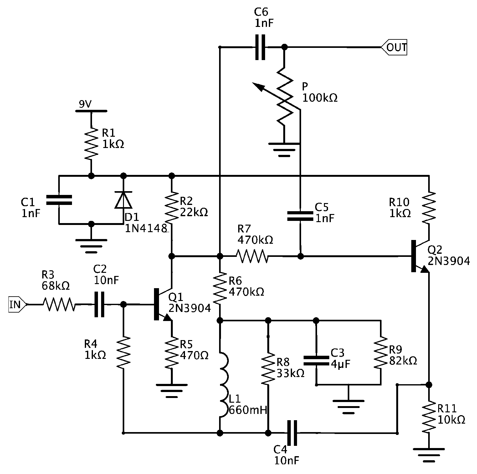
5.3. Wah Pedal
6. Conclusions
- the graph theory to describe the interconnection network of a given circuit’s schematic,
- a dictionary of elementary components which are conformable with PHS formalism.
Acknowledgments
Author Contributions
Conflicts of Interest
Appendix A. Reduction
Appendix B. Dictionary of Elementary Components

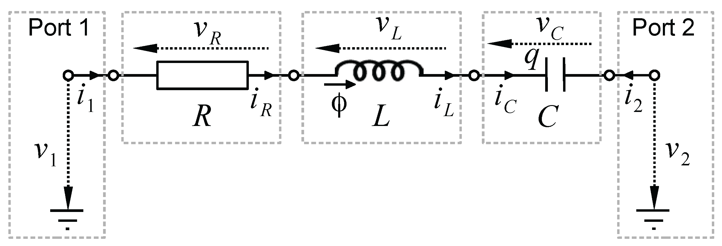
| 2-Ports | |||||
| Storage | Diagram | Stored Energy | Voltage | Current | |
| Inductance |  | ϕ | |||
| Capacitance |  | q | |||
| Dissipative | Diagram | Dissipated Power | Voltage | Current | |
| Resistance |  | i | w | ||
| Conductance |  | v | w | ||
| PN Diode |  | v | w | ||
| 3-Ports | |||||
| Dissipative | Diagram | ||||
| NPN Transistor |  | ||||
| Potentiometer |  | ||||
Appendix B.1. Storage Components
Appendix B.2. Linear Dissipative Components
Appendix B.3. Nonlinear Dissipative Components
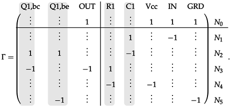
Appendix B.4. Incidence Matrices Γ
Appendix C. Discrete Gradient for Multi-Variate Hamiltonian
References
- Bilbao, S. Sound Synthesis and Physical Modeling. In Numerical Sound Synthesis: Finite Difference Schemes and Simulation in Musical Acoustics; John Wiley & Sons Ltd.: Chichester, UK, 2009. [Google Scholar]
- Bilbao, S. Conservative numerical methods for nonlinear strings. J. Acoust. Soc. Am. 2005, 118, 3316–3327. [Google Scholar] [CrossRef]
- Chabassier, J.; Joly, P. Energy preserving schemes for nonlinear Hamiltonian systems of wave equations: Application to the vibrating piano string. Comput. Methods Appl. Mech. Eng. 2010, 199, 2779–2795. [Google Scholar] [CrossRef]
- Välimäki, V.; Pakarinen, J.; Erkut, C.; Karjalainen, M. Discrete-time modelling of musical instruments. Rep. Prog. Phys. 2006, 69, 1–78. [Google Scholar] [CrossRef]
- Petrausch, S.; Rabenstein, R. Interconnection of state space structures and wave digital filters. IEEE Trans. Circuits Syst. II Express Br. 2005, 52, 90–93. [Google Scholar] [CrossRef]
- Yeh, D.T.; Smith, J.O. Simulating guitar distortion circuits using wave digital and nonlinear state-space formulations. In Proceedings of the 1st International Conference on Digital Audio Effects (DAFx’08), Espoo, Finland, 1–4 September 2008; pp. 19–26.
- Fettweis, A. Wave digital filters: Theory and practice. Proc. IEEE 1986, 74, 270–327. [Google Scholar] [CrossRef]
- Sarti, A.; De Poli, G. Toward nonlinear wave digital filters. IEEE Trans. Signal Process. 1999, 47, 1654–1668. [Google Scholar] [CrossRef]
- Pedersini, F.; Sarti, A.; Tubaro, S. Block-wise physical model synthesis for musical acoustics. Electron. Lett. 1999, 35, 1418–1419. [Google Scholar] [CrossRef]
- Pakarinen, J.; Tikander, M.; Karjalainen, M. Wave digital modeling of the output chain of a vacuum-tube amplifier. In Proceedings of the 12th International Conference on Digital Audio Effects (DAFx’09), Como, Italy, 1–4 September 2009; pp. 1–4.
- De Paiva, R.C.D.; Pakarinen, J.; Välimäki, V.; Tikander, M. Real-time audio transformer emulation for virtual tube amplifiers. EURASIP J. Adv. Signal Process. 2011, 2011, 1–15. [Google Scholar] [CrossRef]
- Fettweis, A. Pseudo-passivity, sensitivity, and stability of wave digital filters. IEEE Trans. Circuit Theory 1972, 19, 668–673. [Google Scholar] [CrossRef]
- Bilbao, S.; Bensa, J.; Kronland-Martinet, R. The wave digital reed: A passive formulation. In Proceedings of the 6th International Conference on Digital Audio Effects (DAFx-03), London, UK, 8–11 September 2003; pp. 225–230.
- Schwerdtfeger, T.; Kummert, A. A multidimensional approach to wave digital filters with multiple nonlinearities. In Proceedings of the 22nd European Signal Processing Conference (EUSIPCO), Lisbon, Portugal, 1–5 September 2014; pp. 2405–2409.
- Werner, K.J.; Nangia, V.; Bernardini, A.; Smith, J.O., III; Sarti, A. An Improved and Generalized Diode Clipper Model for Wave Digital Filters. In Proceedings of the 139th Convention of the Audio Engineering Society (AES), New York, NY, USA, 29 October–1 November 2015.
- Khalil, H.K. Nonlinear Systems; Prentice Hall: Upper Saddle River, NJ, USA, 2002; Volume 3. [Google Scholar]
- Cohen, I.; Helie, T. Real-time simulation of a guitar power amplifier. In Proceedings of the 13th International Conference on Digital Audio Effects (DAFx-10), Graz, Austria, 6–10 September 2010.
- Yeh, D.T.; Abel, J.S.; Smith, J.O. Automated physical modeling of nonlinear audio circuits for real-time audio effects—Part I: Theoretical development. IEEE Trans. Audio Speech Lang. Process. 2010, 18, 728–737. [Google Scholar] [CrossRef]
- Borin, G.; De Poli, G.; Rocchesso, D. Elimination of delay-free loops in discrete-time models of nonlinear acoustic systems. IEEE Trans. Audio Speech Lang. Process. 2000, 8, 597–605. [Google Scholar] [CrossRef]
- Hélie, T. Lyapunov stability analysis of the Moog ladder filter and dissipativity aspects in numerical solutions. In Proceedings of the 14th International Conference on Digital Audio Effects DAFx-11, Paris, France, 19–23 September 2011; pp. 45–52.
- Maschke, B.M.; Van der Schaft, A.J.; Breedveld, P.C. An intrinsic Hamiltonian formulation of network dynamics: Non-standard Poisson structures and gyrators. J. Frankl. Inst. 1992, 329, 923–966. [Google Scholar] [CrossRef]
- Van der Schaft, A.J. Port-Hamiltonian systems: An introductory survey. In Proceedings of the International Congress of Mathematicians, Madrid, Spain, 22–30 August 2006; pp. 1339–1365.
- Stramigioli, S.; Duindam, V.; Macchelli, A. Modeling and Control of Complex Physical Systems: The Port-Hamiltonian Approach; Springer: Berlin, Germany, 2009. [Google Scholar]
- Marsden, J.E.; Ratiu, T.S. Introduction to Mechanics and Symmetry: A Basic Exposition of Classical Mechanical Systems; Springer: New Yor, NY, USA, 1999; Volume 17. [Google Scholar]
- Itoh, T.; Abe, K. Hamiltonian-conserving discrete canonical equations based on variational difference quotients. J. Comput. Phys. 1988, 76, 85–102. [Google Scholar] [CrossRef]
- Tellegen, B.D.H. A general network theorem, with applications. Philips Res. Rep. 1952, 7, 259–269. [Google Scholar]
- Desoer, C.A.; Kuh, E.S. Basic Circuit Theory; Tata McGraw-Hill Education: Noida, India, 2009. [Google Scholar]
- Karnopp, D. Power-conserving transformations: Physical interpretations and applications using bond graphs. J. Frankl. Inst. 1969, 288, 175–201. [Google Scholar] [CrossRef]
- Breedveld, P.C. Multibond graph elements in physical systems theory. J. Frankl. Inst. 1985, 319, 1–36. [Google Scholar] [CrossRef]
- Falaize, A.; Hélie, T. Guaranteed-passive simulation of an electro-mechanical piano: A port-Hamiltonian approach. In Proceedings of the 18th International Conference on Digital Audio Effects (DAFx), Trondheim, Norway, 30 November–3 December 2015.
- Falaize, A.; Lopes, N.; Hélie, T.; Matignon, D.; Maschke, B. Energy-balanced models for acoustic and audio systems: A port-Hamiltonian approach. In Proceedings of the Unfold Mechanics for Sounds and Music, Paris, France, 11–12 September 2014.
- Vladimirescu, A. The SPICE Book; John Wiley & Sons, Inc.: New Yor, NY, USA, 1994. [Google Scholar]
- Diestel, R. Graph Theory, 4th ed.; Springer: New Yor, NY, USA, 2010. [Google Scholar]
- Do Carmo, M.P. Differential Geometry of Curves and Surfaces; Prentice-Hall: Englewood Cliffs, NJ, USA, 1976; Volume 2, p. 131. [Google Scholar]
- Hairer, E.; Lubich, C.; Wanner, G. Geometric Numerical Integration: Structure-Preserving Algorithms for Ordinary Differential Equations; Springer Science & Business Media: New York, NY, USA, 2006; Volume 31. [Google Scholar]
- Oppenheim, A.V.; Schafer, R.W. Discrete-Time Signal Processing, 3rd ed.; Pearson Higher Education: San Francisco, CA, USA, 2010. [Google Scholar]
- Jones, E.; Oliphant, E.; Peterson, P. SciPy: Open Source Scientific Tools for Python, function scipy.optimize.root. Available online: http://docs.scipy.org/doc/scipy/reference/generated/scipy.optimize.root.html#scipy.optimize.root (accessed on 22 September 2016).
- Falaize, A. A comparison of numerical methods. Available online: http://recherche.ircam.fr/anasyn/falaize/applis/comparisonnumschemes/ (accessed on 22 September 2016).
- Yeh, D.T. Automated physical modeling of nonlinear audio circuits for real-time audio effects—Part II: BJT and vacuum tube examples. IEEE Trans. Audio Speech Lang. Process. 2012, 20, 1207–1216. [Google Scholar] [CrossRef]
- Butcher, J.C. Numerical Methods for Ordinary Differential Equations; John Wiley & Sons, Ltd.: London, UK, 2008; p. 26. [Google Scholar]
- Holters, M.; Zölzer, U. Physical Modelling of a Wah–Wah Effect Pedal as a case study for Application of the nodal DK Method to circuits with variable parts. In Proceedings of the 14th International Conference on Digital Audio Effects (DAFx-11), Paris, France, 19–23 September 2011.
- Falaize-Skrzek, A.; Hélie, T. Simulation of an analog circuit of a wah pedal: A port-Hamiltonian approach. In Proceedings of the 135th Convention of the Audio Engineering Society, New York, NY, USA, 17–20 October 2013.
- Steinberg Media Technologies GmbH. Virtual Studio Technology. Available online: http://www.steinberg.net/en/company/technologies/vst3.html (accessed on 22 September 2016).
- ROLI Ltd. The JUCE framework. Available online: http://www.juce.com (accessed on 22 September 2016).
- Falaize, A. Companion web-site to the present article entitled "Passive Guaranteed Simulation of Analog Audio Circuits: A port-Hamiltonian Approach". Available online: http://recherche.ircam.fr/anasyn/falaize/applis/analogcircuits/ (accessed on 22 September 2016).
- Aoues, S. Schémas d’intégration dédiés à l’étude, l’analyse et la synthèse dans le formalisme Hamiltonien à ports. Ph.D. Thesis, INSA, Lyon, France, December 2014; pp. 32–35. [Google Scholar]


| Line | Label | Node List | Type | Parameters |
|---|---|---|---|---|
| CapaLin | ||||
| Resistor | ||||
| NPN_ Type1 | List of parameters | |||
| Vcc | Voltage | 9 | ||
| IN | Voltage | ∼ | ||
| OUT | Current | 0 | ||
| GRD | Voltage | 0 |
| Component type | Current-Controlled | Voltage-Controlled |
|---|---|---|
| storages | capacitor | inductor |
| resistors | resistance | conductance |
| nonlinear | diodes, transistors | |
| sources | voltage source | current source |
| Method | Update |
|---|---|
| Trapezoidal rule | |
| Midpoint rule | |
| PHS with discrete gradient |
© 2016 by the authors; licensee MDPI, Basel, Switzerland. This article is an open access article distributed under the terms and conditions of the Creative Commons Attribution (CC-BY) license (http://creativecommons.org/licenses/by/4.0/).
Share and Cite
Falaize, A.; Hélie, T. Passive Guaranteed Simulation of Analog Audio Circuits: A Port-Hamiltonian Approach. Appl. Sci. 2016, 6, 273. https://doi.org/10.3390/app6100273
Falaize A, Hélie T. Passive Guaranteed Simulation of Analog Audio Circuits: A Port-Hamiltonian Approach. Applied Sciences. 2016; 6(10):273. https://doi.org/10.3390/app6100273
Chicago/Turabian StyleFalaize, Antoine, and Thomas Hélie. 2016. "Passive Guaranteed Simulation of Analog Audio Circuits: A Port-Hamiltonian Approach" Applied Sciences 6, no. 10: 273. https://doi.org/10.3390/app6100273