Magnetohydrodynamic Flow and Heat Transfer of Nanofluids in Stretchable Convergent/Divergent Channels

Abstract

This article is dedicated to analyzing the heat transfer in the flow of water-based nanofluids in a channel with non-parallel stretchable walls. The magnetohydrodynamic (MHD) nature of the flow is considered. Equations governing the flow are transformed into a system of nonlinear ordinary differential equations. The said system is solved by employing two different techniques, the variational iteration method (VIM) and the Runge-Kutta-Fehlberg method (RKF). The influence of the emerging parameters on the velocity and temperature profiles is highlighted with the help of graphs coupled with comprehensive discussions. A comparison with the already existing solutions is also made, which are the special cases of the current problem. It is observed that the temperature profile decreases with an increase in the nanoparticle volume fraction. Furthermore, a magnetic field can be used to control the possible separation caused by the backflows in the case of diverging channels. The effects of parameters on the skin friction coefficient and Nusselt number are also presented using graphical aid. The nanoparticle volume fraction helps to reduce the temperature of the channel and to enhance the rate of heat transfer at the wall.

1. Introduction

Flow through non-parallel walls is an important area of research due to its many practical, industrial, physical and biological applications, such as flows through rivers and canals. Blood also exhibits such a flow, where the arteries and capillaries are linked with each other. Pioneering work in this area was done by Jeffery and Hamel [1,2]. Plenty of studies are available in this area inspecting the various properties of flow by considering various external forces, such as external magnetic fields and the other forces. One can easily find enough literature on this topic in [3,4] and the references therein.

The study of stretching or shrinking sheets has been an area of modern research due to the practical applications in the real world. These applications include glass fiber production, engineering melt spinning, the manufacturing of rubber sheets, etc. The work presented by Crane [5] was the first study on stretching flows. Since then, several researchers from all over the world have used the said problem to formulate and present the various properties of flows over the stretching/shrinking surfaces that can be seen in [6,7,8] and some of the references therein. They used heat and mass transfer effects and analyzed the various properties of flows over stretching/shrinking surfaces.

Traditional fluids, like water, kerosene, ethylene glycol, etc., in general, are not good conductors. To cope with this problem and to enhance the thermal properties of various fluids, Choi [9,10] presented a model that used the term nanofluids. The idea is to add an appropriate amount of nanoparticles to the traditional fluids. The experimental results have proven that the thermal properties of traditional fluids can be enhanced appreciably by using the said technique. After this groundbreaking idea, many models were presented by various researchers that had also incorporated the Brownian motion and thermophoresis effects. Buongiorno [11], Xue [12], Hamilton and Crosser [13] and Maxwell [14] are the major contributors who have presented some useful and efficient models for nanofluids. In recent times, many authors have been inclined to work in the field of nanofluids. Using Buongiorno’s model, Khan et al. [15] extended the work on nanofluids to a stretching surface. Since then, many studies have been presented using the models discussed earlier for different geometries and various types of nanoparticles. One can find enough literature on these topics [16,17,18,19,20,21,22,23,24,25,26,27,28,29,30,31,32,33,34,35].

The complex nature of the equations in daily life problems makes exact solutions least likely. Therefore, many analytical, as well as numerical techniques are developed to solve the problems representing the physical nature. Some of the analytical techniques are Adomian’s decomposition method (ADM), the homotopy perturbation method (HPM), the variational iteration method (VIM), the variation of parameters method (VPM), the homotopy analysis method (HAM), etc. In this article, VIM is successfully applied to the problem, and the efficiency and accuracy of VIM can be seen in [36,37] and the references therein.

In a recent study, Turkyilmazoglu [38] extended the traditional Jeffery-Hamel flow problem to a case incorporating stretching/shrinking walls. He also studied the heat transfer effects on the flow. In the study under consideration, we examined a further extended form of the same problem dealing with the nanofluid flow under the influence of magnetohydrodynamic forces. Due to the very abstract nature of the governing equations and the expected non-availability of the exact solutions, an analytical approximation technique called the variational iteration method (VIM) has been used to approximate the solution. A comparison of analytical results is made with the numerical ones obtained by employing theRunge-Kutta-Fehlberg technique and is presented in the form of tables. Existing solutions (of the limited cases) and the ones obtained in this article are also compared to verify the solutions obtained. A comprehensive graphical description of the effects of the various parameters on the velocity and temperature profiles is presented coupled with some detailed discussions.

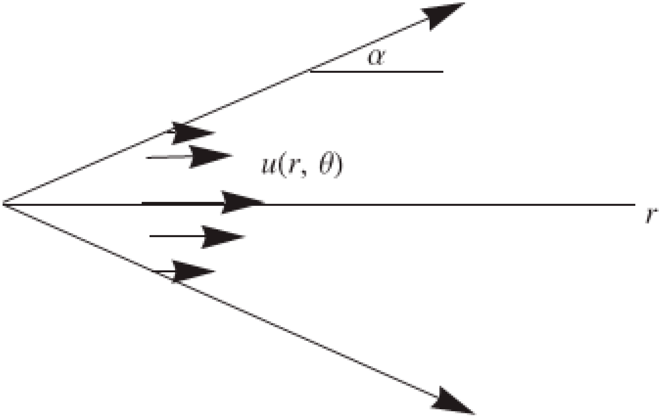
2. Governing Equations

Consider the flow from the source or sink at the intersection of two plane walls. 2α is taken as the angle between the walls, as depicted in Figure 1. The walls are assumed to be stretching/shrinking at a rate $s$in such a way that the velocity at the wall can be written as $\stackrel{\wedge }{u_r}=U_w=\frac{s}{r}$. Furthermore, $\mathsf{\alpha }>0$ represents the case of a divergent channel, while for $\mathsf{\alpha }<0,$ the same channel is convergent. The channel is assumed to be saturated by the nanofluid consisting of water (the base fluid) and the copper (Cu) or silver (Ag) nanoparticles. A thermal equilibrium between the base fluid and the nanoparticles is assumed. A uniform transverse magnetic field of strength $B_0$ is applied across the channel to analyze the flow under the influence of an external body force.

Figure 1. Schematic diagram of the flow problem.

Figure 1. Schematic diagram of the flow problem.

For the said flow, a polar coordinates system $\left(r,\mathsf{\theta }\right)$ is used to formulate the problem. Under the said conventions, the velocity field takes the form V = ($u_r$, 0, 0), where $u_r$ is a function of both $r$ and $\mathsf{\text{θ}}$.

The equations of continuity, momentum and energy in polar coordinates under the imposed assumptions become [38]:

$$\frac{1}{r}\frac{\partial }{\partial r}(r\stackrel{\wedge }{u_r})=0$$

(1)

$${\mathsf{\rho }}_{nf}\left(\stackrel{\wedge }{u_r}\frac{\partial \stackrel{\wedge }{u_r}}{\partial r}\right)=-\frac{\partial p}{\partial r}+{\mathsf{\mu }}_{nf}\left[\frac{{\partial }^2\stackrel{\wedge }{u_r}}{\partial r^2}+\frac{1}{r}\frac{\partial \stackrel{\wedge }{u_r}}{\partial r}+\frac{1}{r^2}\frac{{\partial }^2\stackrel{\wedge }{u_r}}{\partial {\mathsf{\theta }}^2}-\frac{\stackrel{\wedge }{u_r}}{r^2}\right]-\frac{{\mathsf{\sigma }}_{nf}{B}_0^2}{{\mathsf{\rho }}_{nf}{r}^2}\stackrel{\wedge }{u_r}$$

(2)

$$-\frac{1}{{\mathsf{\rho }}_{nf}r}\frac{\partial p}{\partial r}+\frac{2}{r^2}\frac{{\mathsf{\mu }}_{nf}}{{\mathsf{\rho }}_{nf}}\frac{\partial \stackrel{\wedge }{u_r}}{\partial \mathsf{\theta }}=0$$

(3)

$$\stackrel{\wedge }{u_r}\frac{\partial \stackrel{\wedge }{T}}{\partial r}=\frac{k_{nf}}{{\left(\mathsf{\rho }{C}_p\right)}_{nf}}\left[\frac{{\partial }^2\stackrel{\wedge }{T}}{\partial r^2}+\frac{1}{r}\frac{\partial \stackrel{\wedge }{T}}{\partial r}+\frac{1}{r^2}\frac{{\partial }^2\stackrel{\wedge }{T}}{\partial {\mathsf{\theta }}^2}\right]+\frac{{\mathsf{\mu }}_{nf}}{{\left(\mathsf{\rho }{C}_p\right)}_{nf}}\left[4{\left(\frac{\partial \stackrel{\wedge }{u_r}}{\partial r}\right)}^2+\frac{1}{r^2}{\left(\frac{\partial \stackrel{\wedge }{u_r}}{\partial \mathsf{\theta }}\right)}^2\right]$$

(4)

Boundary conditions for the problem are:

$$\begin{array}{c}\stackrel{\wedge }{u_r}=\frac{U_c}{r},\hspace{1em}\frac{\partial \stackrel{\wedge }{u_r}}{\partial \mathsf{\theta }}=0,\hspace{1em}\frac{\partial \stackrel{\wedge }{T}}{\partial \mathsf{\theta }}=0 \mathrm{at}\mathsf{\theta }=0\\ \stackrel{\wedge }{u_r}=U_w=\frac{s}{r},\hspace{1em}\hspace{1em}\stackrel{\wedge }{T}=\frac{\stackrel{\wedge }{T_w}}{r^2} \mathrm{at}\mathsf{\theta }=\pm \mathsf{\alpha }\end{array}$$

(5)

where $U_c$ is the velocity at the centerline of the channel and $U_w$, ${\stackrel{\wedge }{T}}_w$, respectively, represent the velocity and temperature at the wall of the channel.

Further, ${\mathsf{\rho }}_{nf}$, ${\mathsf{\mu }}_{nf}$, ${\mathsf{\sigma }}_{nf}$, ${\left(\mathsf{\rho }{C}_p\right)}_{nf}$ and $k_{nf}$ denote the density, dynamic viscosity, electric conductivity, heat capacity and the thermal conductivity of the fluid, respectively [27,28,29]; where,

$${\mathsf{\upsilon }}_{nf}=\frac{{\mathsf{\mu }}_{nf}}{{\mathsf{\rho }}_{nf}},{\mathsf{\mu }}_{nf}=\frac{{\mathsf{\mu }}_f}{{\left(1-\mathsf{\phi }\right)}^{2.5}},{\mathsf{\alpha }}_{nf}=\frac{k_{nf}}{{\left(\mathsf{\rho }{C}_p\right)}_{nf}},{\mathsf{\rho }}_{nf}=\left(1-\mathsf{\phi }\right)+\mathsf{\phi }\frac{{\mathsf{\rho }}_s}{{\mathsf{\rho }}_f},{\left(\mathsf{\rho }{C}_p\right)}_{nf}=\left(1-\mathsf{\phi }\right)+\mathsf{\phi }\frac{{\left(\mathsf{\rho }{C}_p\right)}_s}{{\left(\mathsf{\rho }{C}_p\right)}_f}$$

The Maxwell-Garnett model for the effective thermal conductivity of nanofluids is used in this problem as [14]:

$$\frac{k_{nf}}{k_f}=\frac{k_s+2k_f-2\mathsf{\phi }\left(k_f-k_s\right)}{k_s+2k_f+\mathsf{\phi }\left(k_f-k_s\right)}$$

(6)

As proposed by Maxwell [18], the effective electrical conductivity of the nanofluid can be written as:

$$\frac{{\mathsf{\sigma }}_{nf}}{{\mathsf{\sigma }}_f}=1+\frac{3\left(\frac{{\mathsf{\sigma }}_s}{{\mathsf{\sigma }}_f}-1\right)\mathsf{\phi }}{\left(\frac{{\mathsf{\sigma }}_s}{{\mathsf{\sigma }}_f}+2\right)-\left(\frac{{\mathsf{\sigma }}_s}{{\mathsf{\sigma }}_f}-1\right)\mathsf{\phi }}$$

(7)

Here, ${\mathsf{\mu }}_f$ is the viscosity of the base fluid and $\mathsf{\phi }$ is the volume fraction for the nanoparticles. $k_f$, $k_s$ are the thermal conductivities, and ${\mathsf{\rho }}_f$, ${\mathsf{\rho }}_s$ are the densities of the base fluid and nanoparticles, respectively. Furthermore, ${\mathsf{\sigma }}_f$ and ${\mathsf{\sigma }}_s$, in order, represent the electrical conductivity of the base fluid and nanoparticles.

The continuity equation (Equation (1)) gives a clear description of the radial velocity of the form,

$$f(\mathsf{\theta })=r\stackrel{\wedge }{u_r}\left(r,\mathsf{\theta }\right)$$

(8)

Using the following non-dimensional variables,

$$F(\mathsf{\eta })=\frac{f(\mathsf{\theta })}{U_c}, \mathsf{\eta }=\frac{\mathsf{\theta }}{\mathsf{\alpha }},\text{Θ}=r^2\frac{T}{T_w}$$

(9)

Elimination of the pressure terms from Equations (2) and (3) and the implementation of similarity transform Equation (9) gives us the coupled equations for the velocity and temperature profiles as:

$$F‴(\mathsf{\eta })+2\mathsf{\alpha }\mathrm{Re}{\left(1-\mathsf{\phi }\right)}^{2.5}{K}_{1}F(\mathsf{\eta })F\prime (\mathsf{\eta })+(4-Ha{\left(1-\mathsf{\phi }\right)}^{2.5}{A}_1){\mathsf{\alpha }}^{2}F\prime (\mathsf{\eta })=0$$

(10)

$${\text{Θ}}^{″}\left(\mathsf{\text{η}}\right)+4{\alpha }^2\text{Θ}\left(\mathsf{\text{η}}\right)+\frac{2K_{2}Pr}{K_3}{\mathsf{\text{α}}}^2\text{Θ}\left(\mathsf{\text{η}}\right)F\left(\mathsf{\text{η}}\right)+\frac{K_{2}EcPr}{K_{3}Re{\left(1-\mathsf{\varphi }\right)}^{2.5}}\left[4{\mathsf{\text{α}}}^2{F}^2\left(\mathsf{\text{η}}\right)+{\left(F^{\prime }\left(\mathsf{\text{η}}\right)\right)}^2\right]=0$$

(11)

Use of Equation (9) reduces the boundary conditions for the problem to a more compact form as:

$$F(0)=1,\hspace{1em}F\prime (0)=0,\hspace{1em}F(1)=S \text{Θ}\prime \left(0\right)=0,\text{Θ}\left(1\right)=1$$

(12)

In the above equations, $S$ denotes the stretching/shrinking parameter and $S>0$ stands for stretchable walls, while $S<0$ represents the case of shrinking walls. Re here is the Reynolds number given by:

$$\mathrm{Re}=\frac{U_c\mathsf{\alpha }}{{\mathsf{\upsilon }}_f}\left(\begin{array}{l}DivergentChannel: \mathsf{\alpha }>0,U>0\\ ConvergentChannel:\mathsf{\alpha }<0,U<0\end{array}\right)$$

Further, $Ha=\sqrt{\frac{{\mathsf{\sigma }}_f{\mathbf{B}}_0^2}{{\mathsf{\mu }}_f}}$, $Ec=\frac{{U_c}^2\mathsf{\alpha }}{{\left(C_p\right)}_f{T}_w}$, $\mathrm{Pr}=\frac{{\left(\mathsf{\rho }{C}_p\right)}_f{U}_c}{k_{\mathsf{\eta }f}}$ represent the Hartmann number, the Eckert number and the Prandtl number, respectively; also:

$$K_1=\left(\left(1-\mathsf{\phi }\right)+\mathsf{\phi }\frac{{\mathsf{\rho }}_s}{{\mathsf{\rho }}_f}\right),K_2=\left(1-\mathsf{\phi }\right)+\mathsf{\phi }\frac{{\left(\mathsf{\rho }{C}_p\right)}_s}{{\left(\mathsf{\rho }{C}_p\right)}_f},K_3=\frac{k_{nf}}{k_f}=\frac{k_s+2k_f-2\mathsf{\phi }\left(k_f-k_s\right)}{k_s+2k_f+\mathsf{\phi }\left(k_f-k_s\right)},A_1=\frac{{\mathsf{\sigma }}_{nf}}{{\mathsf{\sigma }}_f}=1+\frac{3\left(\frac{{\mathsf{\sigma }}_s}{{\mathsf{\sigma }}_f}-1\right)\mathsf{\phi }}{\left(\frac{{\mathsf{\sigma }}_s}{{\mathsf{\sigma }}_f}+2\right)-\left(\frac{{\mathsf{\sigma }}_s}{{\mathsf{\sigma }}_f}-1\right)\mathsf{\phi }}$$

Quantities of physical interest are the skin friction coefficient and the Nusselt number, defined as:

$$C_F=\frac{{\mathsf{\mu }}_{nf}{\left({\mathsf{\tau }}_{r\mathsf{\theta }}\right)}_{\mathsf{\eta }=1}}{{\mathsf{\rho }}_{nf}{U}^2},Nu=\frac{-l{k}_f{\left(q_w\right)}_{\mathsf{\eta }=1}}{k{T}_w}$$

In terms of Equations (8)–(11), we have:

$${\mathrm{Re}}_r{C}_f=\frac{1}{K_1{\left(1-\mathsf{\phi }\right)}^{2.5}}F\prime (1)$$

(13)

$$\mathsf{\text{α}}Nu=-K_3\text{Θ}\prime \left(1\right)$$

(14)

3. Solution Procedure

The solution of the system of equations governing the flow is obtained by using VIM. Implementing the traditional form of VIM, the velocity and temperature profiles in recursive form can be written in the form,

$$\begin{array}{ll}{F}_{n+1}\left(\mathsf{\eta }\right)& =F_n\left(\mathsf{\eta }\right)\\ & +{\displaystyle \underset{0}{\overset{\mathsf{\eta }}{\mathsf{\int }}}{\mathsf{\lambda }}_F\left(s\right)\left(F‴\left(s\right)+\left(4-{\left(1-\mathsf{\phi }\right)}^{2.5}{A}_{1}Ha\right){\mathsf{\alpha }}^2\tilde{F}\prime \left(s\right)+{\left(1-\mathsf{\phi }\right)}^{2.5}{A}_{1}2\mathsf{\alpha }\mathrm{Re}\tilde{F}\left(s\right)\tilde{F}\prime \left(s\right)\right)}ds\end{array}$$

(15)

$${\text{Θ}}_{n+1}\left(\mathsf{\text{η}}\right)={\text{Θ}}_n\left(\mathsf{\text{η}}\right){{\displaystyle \int }}_0^{\mathsf{\text{η}}}{\text{λ}}_{\text{Θ}}\left[\begin{array}{c}[\mathrm{\Theta }″\left(s\right)+4{\mathsf{\text{α}}}^2\mathrm{\Theta }\left(s\right)+\frac{2K_{2}Pr}{K_3}{\mathsf{\text{α}}}^2\mathrm{\Theta }\left(s\right)F\left(s\right)\\ \frac{K_{2}EcPr}{K_{3}Re{\left(1-\mathsf{\varphi }\right)}^{2.5}}\left[4{\mathsf{\text{α}}}^2{F}^2\left(s\right)+{\left(F^{\prime }\left(s\right)\right)}^2\right]\end{array}\right]ds$$

(16)

where the Lagrange multipliers for velocity and temperature profile are ${\mathsf{\lambda }}_F\left(s\right)$ and ${\lambda }_{\text{Θ}}\left(s\right)$, respectively. Approximate Lagrange multipliers for the above problem can be obtained using the variational approach as ${\mathsf{\lambda }}_F\left(s\right)=-\frac{{\left(s-\mathsf{\eta }\right)}^2}{2!}$ and ${\lambda }_{\text{Θ}}\left(s\right)=\left(s-\mathsf{\text{η}}\right)$, so that the above iterative scheme can be reformulated as:

$$\begin{array}{ll}{F}_{n+1}\left(\mathsf{\eta }\right)& =F_n\left(\mathsf{\eta }\right)\\ & -{\displaystyle \underset{0}{\overset{\mathsf{\eta }}{\int }}\frac{{\left(s-\mathsf{\eta }\right)}^2}{2!}\left(F‴\left(s\right)+\left(4-{\left(1-\mathsf{\phi }\right)}^{2.5}{A}_{1}Ha\right){\mathsf{\alpha }}^{2}F\prime \left(s\right)+{\left(1-\mathsf{\phi }\right)}^{2.5}{K}_{1}2\mathsf{\alpha }\mathrm{Re}F\left(s\right)F\prime \left(s\right)\right)}ds\end{array}$$

$$\begin{array}{c}{\mathrm{\Theta }}_{n+1}\left(\mathsf{\eta }\right)={\mathrm{\Theta }}_n\left(\mathsf{\eta }\right)\\ +{{\displaystyle \int }}_0^{\eta }\left(s-\mathsf{\eta }\right)\left[\begin{array}{c}[\mathrm{\Theta }″\left(\mathsf{\eta }\right)+4{\mathsf{\alpha }}^2\mathrm{\Theta }\left(\mathsf{\eta }\right)+\frac{2K_{2}Pr}{K_3}{\mathsf{\alpha }}^2\mathrm{\Theta }\left(\mathsf{\eta }\right)F\left(\mathsf{\eta }\right)\\ \frac{K_{2}EcPr}{K_{3}Re{\left(1-\mathsf{\varphi }\right)}^{2.5}}\left[4{\mathsf{\alpha }}^2{F}^2\left(\mathsf{\eta }\right)+{\left(F^{\prime }\left(\mathsf{\eta }\right)\right)}^2\right]\end{array}\right]ds\\ +{{\displaystyle \int }}_0^{\eta }\left(s-\mathsf{\eta }\right)\left[\begin{array}{c}[\mathrm{\Theta }″\left(\mathsf{\eta }\right)+4{\mathsf{\alpha }}^2\mathrm{\Theta }\left(\mathsf{\eta }\right)+\frac{2K_{2}Pr}{K_3}{\mathsf{\alpha }}^2\mathrm{\Theta }\left(\mathsf{\eta }\right)F\left(\eta \right)\\ \frac{K_{2}EcPr}{K_{3}Re{\left(1-\mathsf{\varphi }\right)}^{2.5}}\left[4{\mathsf{\alpha }}^2{F}^2\left(\mathsf{\eta }\right)+{\left(F^{\prime }\left(\mathsf{\eta }\right)\right)}^2\right]\end{array}\right]ds\end{array}$$

For the initial guess, using boundary conditions for velocity and temperature profiles, we get:

$$F_0\left(\mathsf{\eta }\right)=1+\mathsf{\beta }\frac{{\mathsf{\eta }}^2}{2},$$

$${\text{Θ}}_0\left(\mathsf{\text{η}}\right)=\mathsf{\text{γ}}$$

where $\mathsf{\beta }$ and $\mathsf{\gamma }$ are the constants that will be calculated by using the boundary conditions $F\left(1\right)=S$ and $\text{Θ}\left(1\right)=1$.

Next, a few terms of the solution are given as:

$$\begin{array}{ll}{F}_1\left(\mathsf{\eta }\right)=1+& \frac{\mathsf{\beta }{\mathsf{\eta }}^2}{2}-0.008333333333333318Re\mathsf{\alpha }{\mathsf{\beta }}^2{\mathsf{\eta }}^6{(1.-1.\mathsf{\varphi })}^{2.5}{K}_1\\ & +{\mathsf{\eta }}^4(-0.16666666666666674{\mathsf{\alpha }}^2\\ & +0.041666666666666685\mathrm{Ha}{\mathsf{\alpha }}^2\mathsf{\beta }{(1.-1.\mathsf{\varphi })}^{2.5}{A}_1\\ & -0.08333333333333337\mathit{Re}\mathsf{\alpha }\mathsf{\beta }{(1.-1.\mathsf{\varphi })}^{2.5}{K}_1)\end{array}$$

$$\begin{array}{ll}{\text{Θ}}_0(\mathsf{\text{η}})=\mathsf{\text{γ}}+{\mathsf{\text{η}}}^2& (-2.{\mathsf{\text{α}}}^2\mathsf{\text{γ}}-\frac{1.\mathrm{Pr}{\mathsf{\text{α}}}^2\mathsf{\text{γ}}{\text{K}}_2}{K_3}-\frac{2.\mathrm{EcPr}{\mathsf{\text{α}}}^2{K}_2}{{(1.-1.\mathsf{\varphi })}^{2.5}{K}_3})\\ & +{\mathsf{\text{η}}}^4(-\frac{0.08333333333333331\mathrm{Pr}{\mathsf{\text{α}}}^2\mathsf{\beta }\mathsf{\text{γ}}{K}_2}{K_3}\\ & -\frac{0.33333333333333326\mathrm{EcPr}{\mathsf{\text{α}}}^2\mathsf{\text{β}}{K}_2}{{(1.-1.\mathsf{\varphi })}^{2.5}{K}_3}\\ & -\frac{0.08333333333333331\mathrm{EcPr}{\mathsf{\text{β}}}^2{K}_2}{{(1.-1.\mathsf{\varphi })}^{2.5}{K}_3})\\ & -\frac{0.033333333333333354\mathrm{EcPr}{\mathsf{\text{α}}}^2{\mathsf{\text{β}}}^2{\mathsf{\text{η}}}^6{K}_2}{{(1.-1.\mathsf{\varphi })}^{2.5}{K}_3}\end{array}$$

(17)

For the sake of simplicity, other iterations of the solutions are omitted here. One can calculate the next iterations in a similar manner.

4. Results and Discussion

To study the flow behavior and the variations in velocity and temperature due to the varying values of the involved parameters, this section is divided into two subsections. One is for the velocity profile, and the other is for the temperature distribution. Both the stretching and shrinking cases combined with the convergence or the divergence of the channel are discussed in detail using the graphical aid. As water is taken to be the base fluid, the numerical values of the Prandtl number Pr shall be fixed at 6.2 throughout the study, unless stated otherwise. Copper (Cu) and silver (Ag) are the nanoparticles incorporated in the base fluid. The thermophysical properties of the base fluid and the nanoparticles are highlighted in Table 1. Furthermore, in all of the graphical descriptions, a solid line represents the graph for Cu, while the dashed line represents the same for Ag.

Table 1. Thermophysical properties of water, copper and silver nanoparticles [22].

	$\mathit{\rho }\mathbf{\left(}\mathit{k}\mathit{g}\mathbf{/}{\mathit{m}}^{\mathbf{3}} \mathbf{\right)}$	${\mathit{C}}_{\mathit{p}}\mathbf{\left(}\mathit{J}\mathbf{/}\mathit{K}\mathit{g}\mathit{K}\mathbf{\right)}$	$\mathit{k}\mathbf{\left(}\mathit{W}\mathbf{/}\mathit{m}\mathit{K}\mathbf{\right)}$	Electrical Conductivity $\mathsf{\sigma }{(\mathbf{\text{Ω}}\mathit{m})}^{\mathbf{-}\mathbf{1}}$
Pure Water	997.1	4179	0.613	0.05
Copper (Cu)	8933	385	401	5.96 × 107
Silver	10,500	235	429	6.3 × 107

Table 1. Thermophysical properties of water, copper and silver nanoparticles [22].

	$\mathit{\rho }\mathbf{\left(}\mathit{k}\mathit{g}\mathbf{/}{\mathit{m}}^{\mathbf{3}} \mathbf{\right)}$	${\mathit{C}}_{\mathit{p}}\mathbf{\left(}\mathit{J}\mathbf{/}\mathit{K}\mathit{g}\mathit{K}\mathbf{\right)}$	$\mathit{k}\mathbf{\left(}\mathit{W}\mathbf{/}\mathit{m}\mathit{K}\mathbf{\right)}$	Electrical Conductivity $\mathsf{\sigma }{(\mathbf{\text{Ω}}\mathit{m})}^{\mathbf{-}\mathbf{1}}$
Pure Water	997.1	4179	0.613	0.05
Copper (Cu)	8933	385	401	5.96 × 107
Silver	10,500	235	429	6.3 × 107

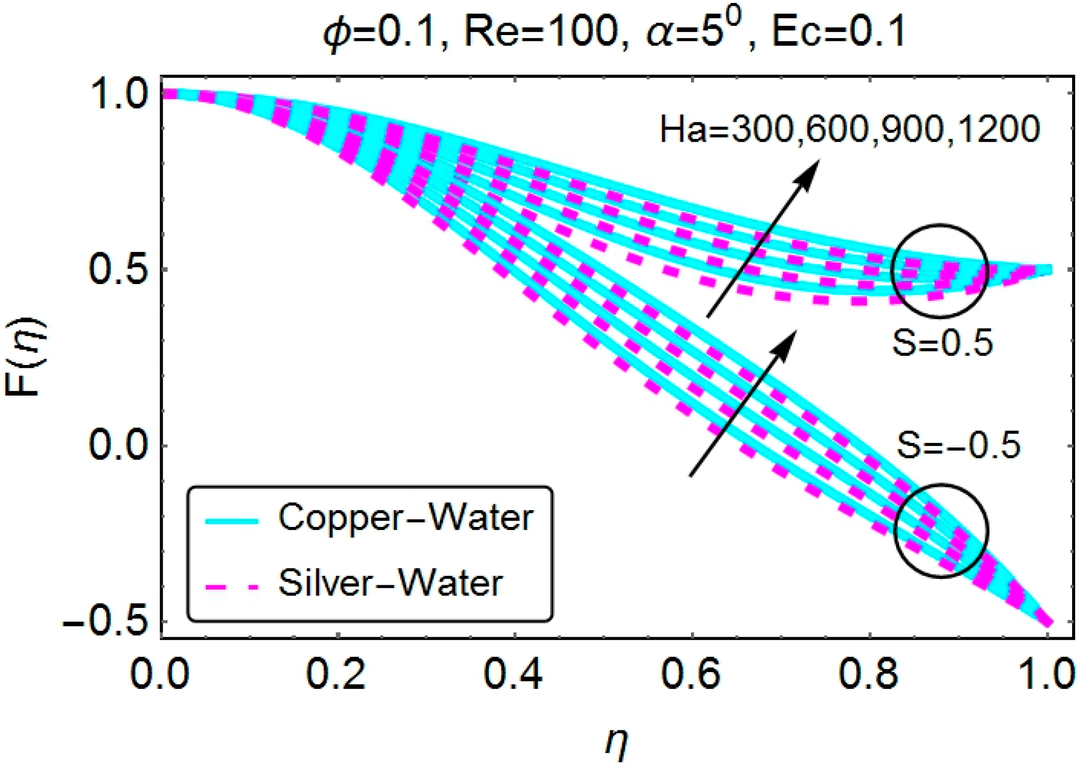
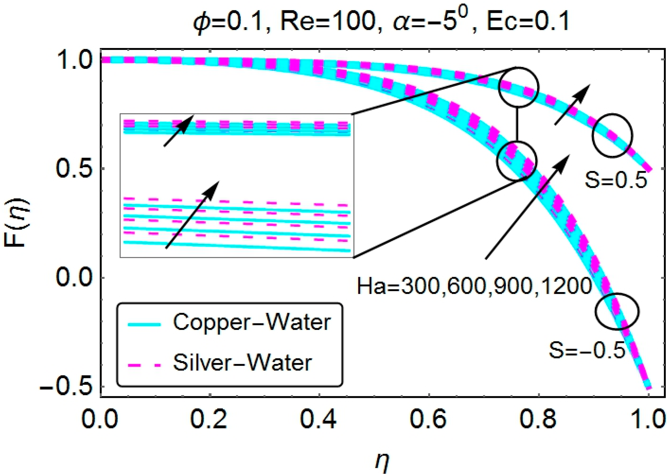
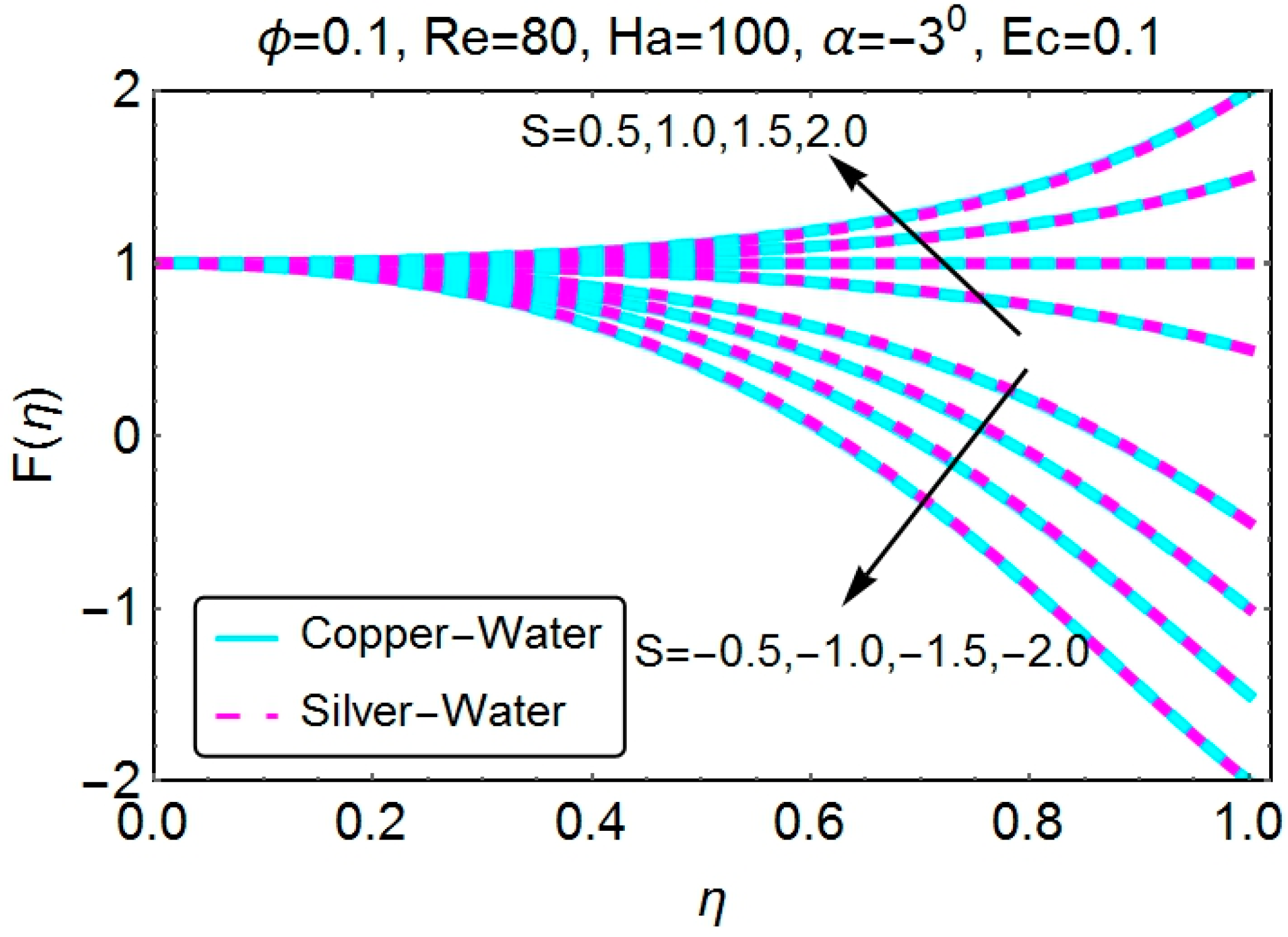
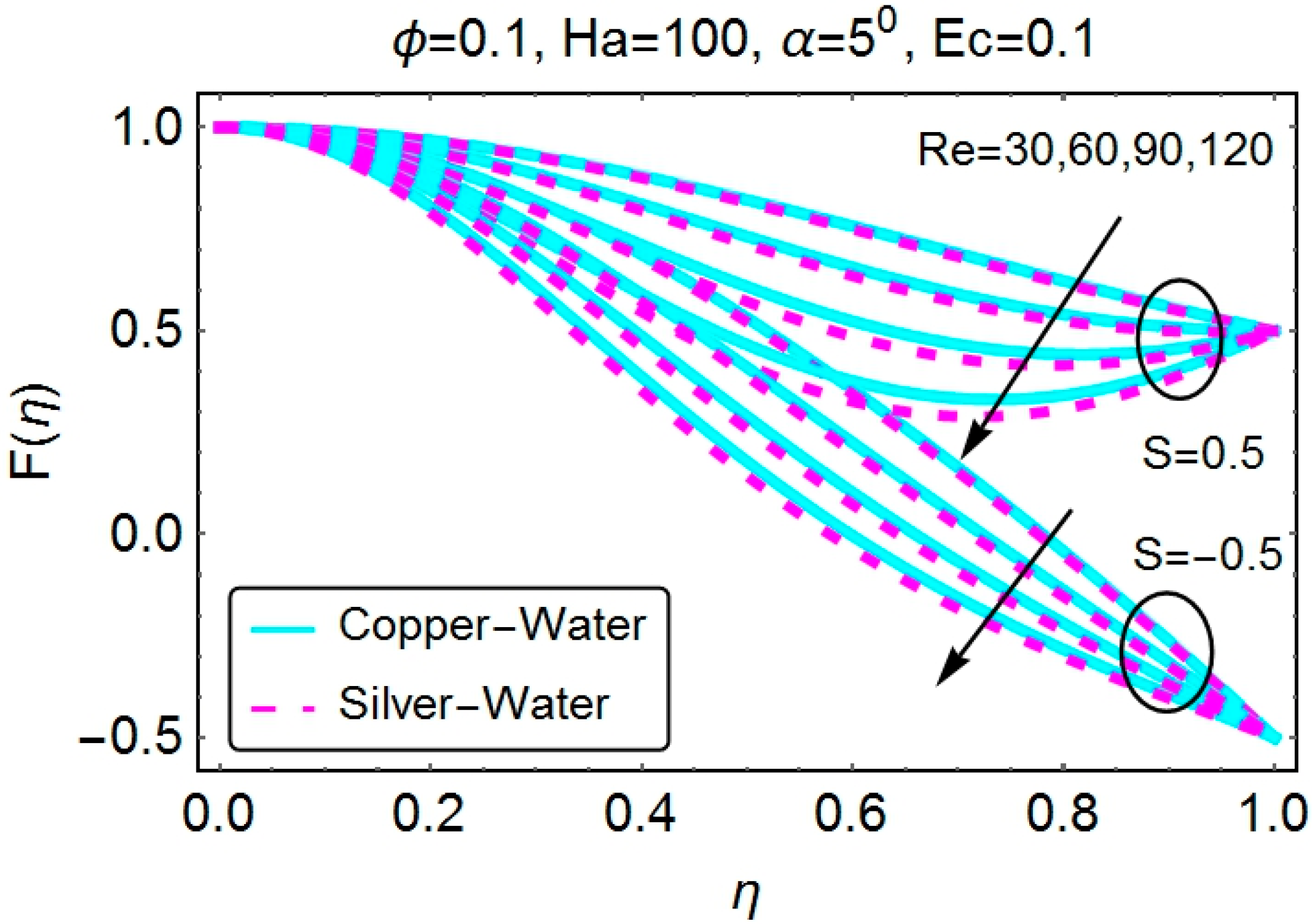
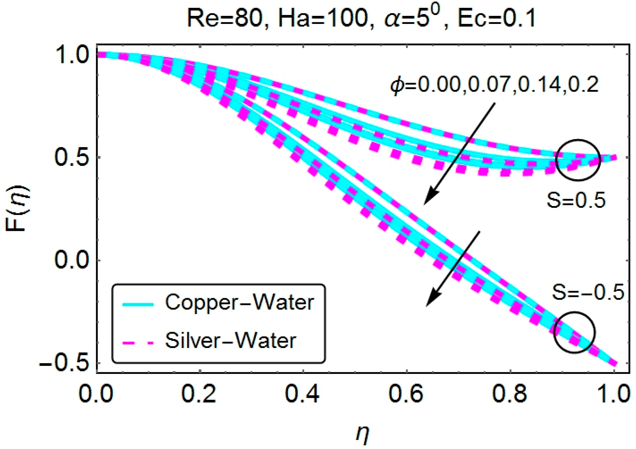
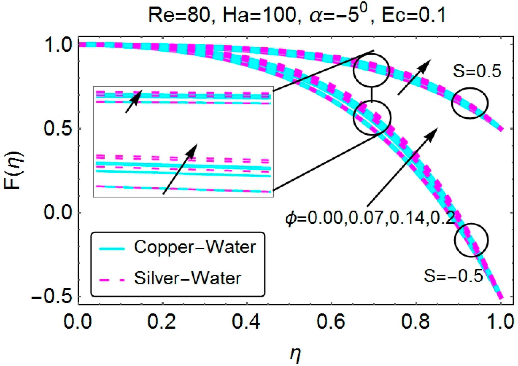
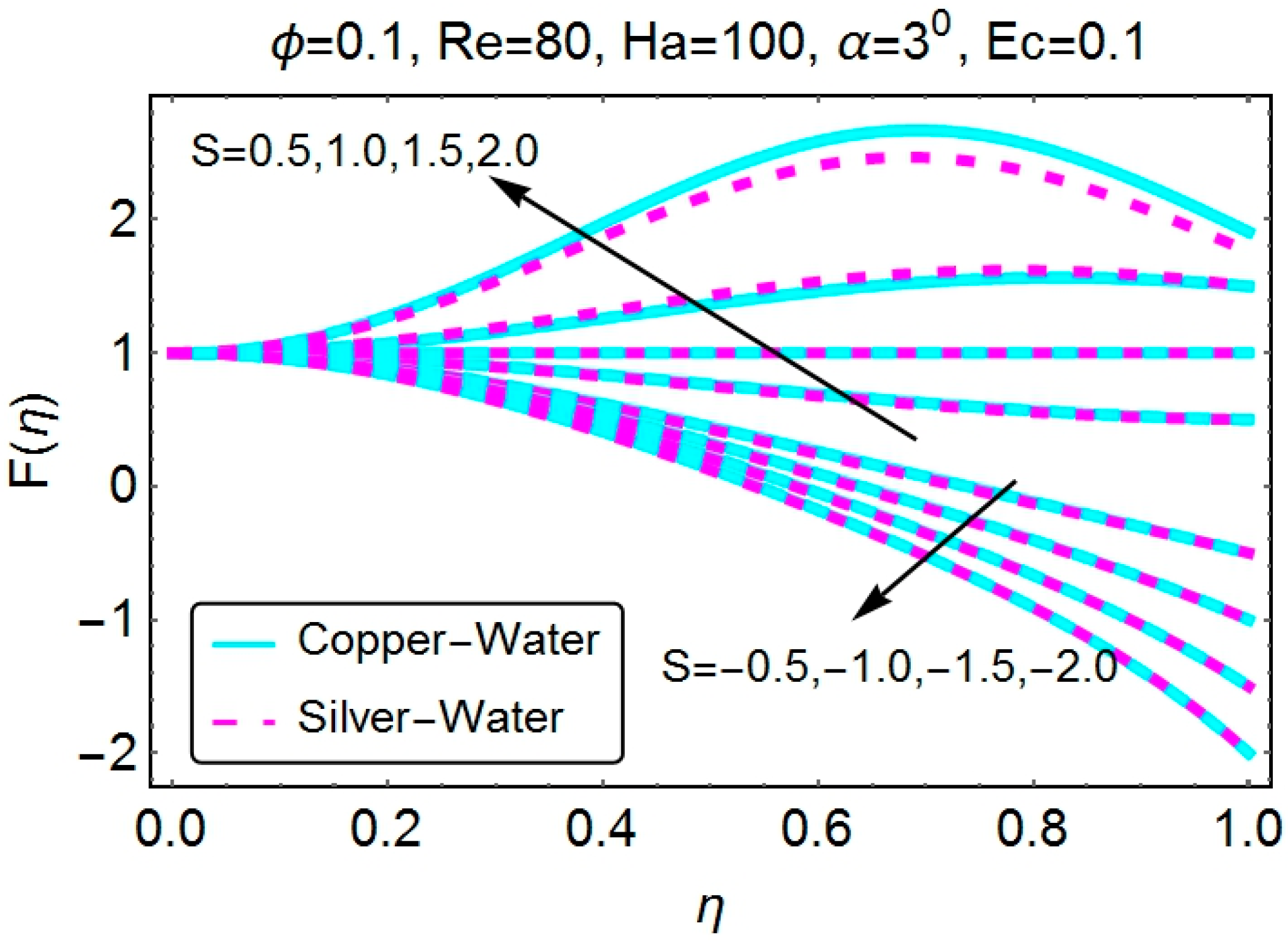
4.1. Velocity Profile

This section is dedicated to exploring the behavior of the velocity profile for both convergent and divergent channels under the variations in the parameters, like the channel opening$\mathsf{\text{α}}$, the Reynolds number$Re$, the volume fraction of nanoparticles ϕ, the Hartmann number$Ha$ and the stretching/shrinking parameter S. For the said purpose, Figure 2, Figure 3, Figure 4, Figure 5, Figure 6, Figure 7, Figure 8, Figure 9, Figure 10 and Figure 11 are plotted. Figure 2 gives a graphical description of the variations in the velocity profile for a divergent channel for different values of channel openin$\mathsf{\text{α}}$. Both the stretching and shrinking cases are discussed in the same figure. A clear drop in the velocity profile is evident for increasing values of α. Here, clearly, for the stretching walls, the change in velocity is seen to be quite rapid at the central portion; there comes a point at which the backflow phenomena are observed particularly for $\mathsf{\text{α}}=5^{°}$. This backflow behavior may result in separation at some point. In Figure 3, the same effects of α for the convergent channel are portrayed. A quite opposite behavior is observed for this case, and increasing values of velocity are observed. For the stretching walls, the change in velocity is on the lower side as compared to the shrinking walls. This means that for a shrinking, convergent channel, more fluid is moved towards the walls as compared to the same for a diverging channel. Copper nanoparticles are seen to have a slightly higher velocity for divergent channels as compared to the silver nanoparticles. The behavior is reversed for a convergent channel.

Figure 2. Change in velocity for varying $\mathsf{\alpha }$ (divergent channel).

Figure 2. Change in velocity for varying $\mathsf{\alpha }$ (divergent channel).

Figure 3. Change in velocity for varying $\mathsf{\alpha }$ (convergent channel).

Figure 3. Change in velocity for varying $\mathsf{\alpha }$ (convergent channel).

Figure 4. Change in velocity for varying $\mathrm{Re}$ (divergent channel).

Figure 4. Change in velocity for varying $\mathrm{Re}$ (divergent channel).

Figure 5. Change in velocity for varying $\mathrm{Re}$ (convergent channel).

Figure 5. Change in velocity for varying $\mathrm{Re}$ (convergent channel).

Figure 6. Change in velocity for varying $Ha$ (divergent channel).

Figure 6. Change in velocity for varying $Ha$ (divergent channel).

Figure 7. Change in velocity for varying $Ha$ (convergent channel).

Figure 7. Change in velocity for varying $Ha$ (convergent channel).

Figure 8. Change in velocity for varying $\mathsf{\phi }$ (divergent channel).

Figure 8. Change in velocity for varying $\mathsf{\phi }$ (divergent channel).

Figure 9. Change in velocity for varying $\mathsf{\phi }$ (convergent channel).

Figure 9. Change in velocity for varying $\mathsf{\phi }$ (convergent channel).

Figure 10. Change in velocity for varying $S$ (divergent channel).

Figure 10. Change in velocity for varying $S$ (divergent channel).

Figure 11. Change in velocity for varying $S$ (convergent channel).

Figure 11. Change in velocity for varying $S$ (convergent channel).

The velocity profile for the increasing values of the Reynolds number Re for the case of a divergent channel is plotted in Figure 4. The higher the values of Re, the lower the velocity becomes in the diverging channel. This results in a backflow near the walls of the channel for stretching walls. A steep decrease in velocity is seen for the stretching/diverging channel as compared to the shrinking one. A quite opposite scenario is seen for the convergent channel, and velocity is an increasing function of Re. This entire discussion shows that the upsurge in viscous forces results in lower values of the Reynolds number, and an increase in the mainstream velocity of the channel increases the values of Re that result in the increasing of the velocity for convergent channels and a decrease in velocity for the divergent channel. Again, for increasing Re, the copper nanoparticles have slightly higher values for the velocity of the divergent channel. This is due to the lower density of copper as compared to silver.

The Hartmann number that represents the strength of the magnetic field results in a growth in the velocity profile when the channel is divergent, as is clear from Figure 6. The behavior is similar for both the stretching and shrinking of walls. Furthermore, whenever there is a backflow in the divergent channel, the Hartmann number can be used to reduce the backflows. It controls the separation phenomena, resulting in a much smoother flow. The velocity behaves in a similar manner for a convergent channel and the increasing values of Ha. However, in this case, the change is slower as compared to the divergent channel. Furthermore, a stretching/converging channel has lower variations in velocity as compared to the shrinking channel (see Figure 7).

To discuss the strength of nanoparticles on the velocity, Figure 8 and Figure 9 are portrayed. A rise in the nanoparticle volume fraction reduces the velocity in a divergent channel. For the stretching of a divergent channel, again, a backflow is observed. However, when the channel is shrinking, there is no backflow. Again, a slightly higher value of the velocity can be observed for the copper nanoparticles than the silver nanoparticles. From all of this, one can easily say for a divergent channel that the higher volume fraction of the nanoparticles provides a low speed flow. On the other hand, a slow rise in the velocity for a convergent channel is evident: it keeps growing with the rising nanoparticle volume fraction.

The influence of stretching and shrinking parameter $S$ on the velocity profile is depicted in Figure 10 and Figure 11. For a divergent channel, an upsurge in the velocity is witnessed. The stretching of a divergent channel marks a higher velocity near the walls as compared to the center of the channel. On the contrary, when a divergent channel is shrinking, the velocity decreases quite sharply near the walls, as shown in Figure 10. In Figure 11, the effects of the same parameter on a convergent channel are portrayed. It gives a clear picture of an accelerated flow near the walls for a stretching channel. On the contrary, a significant decrease in velocity is seen in a convergent channel with shrinking walls. For both of these cases, the changes are quite prominent near the walls of the channel. As we move towards the center, the effects get weaker and less influential.

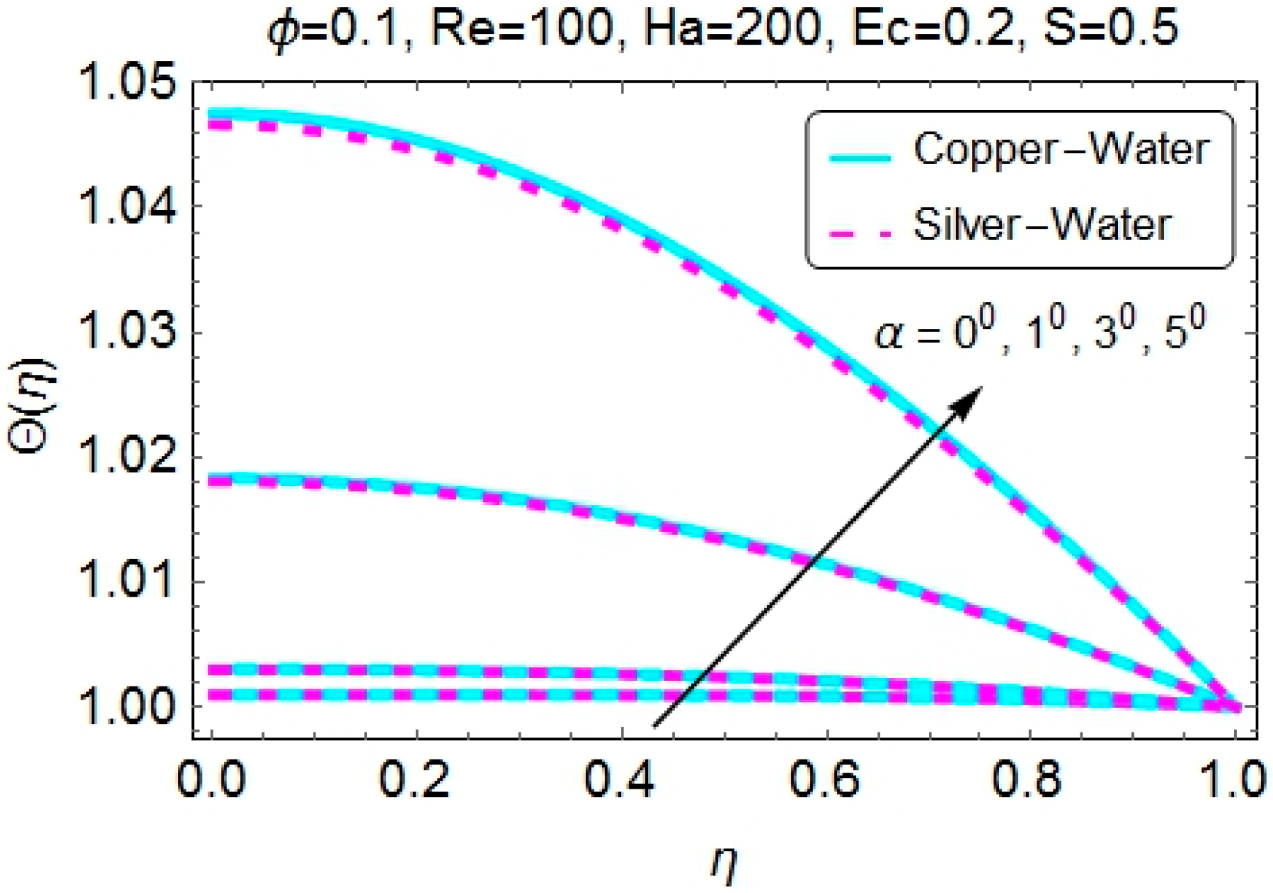
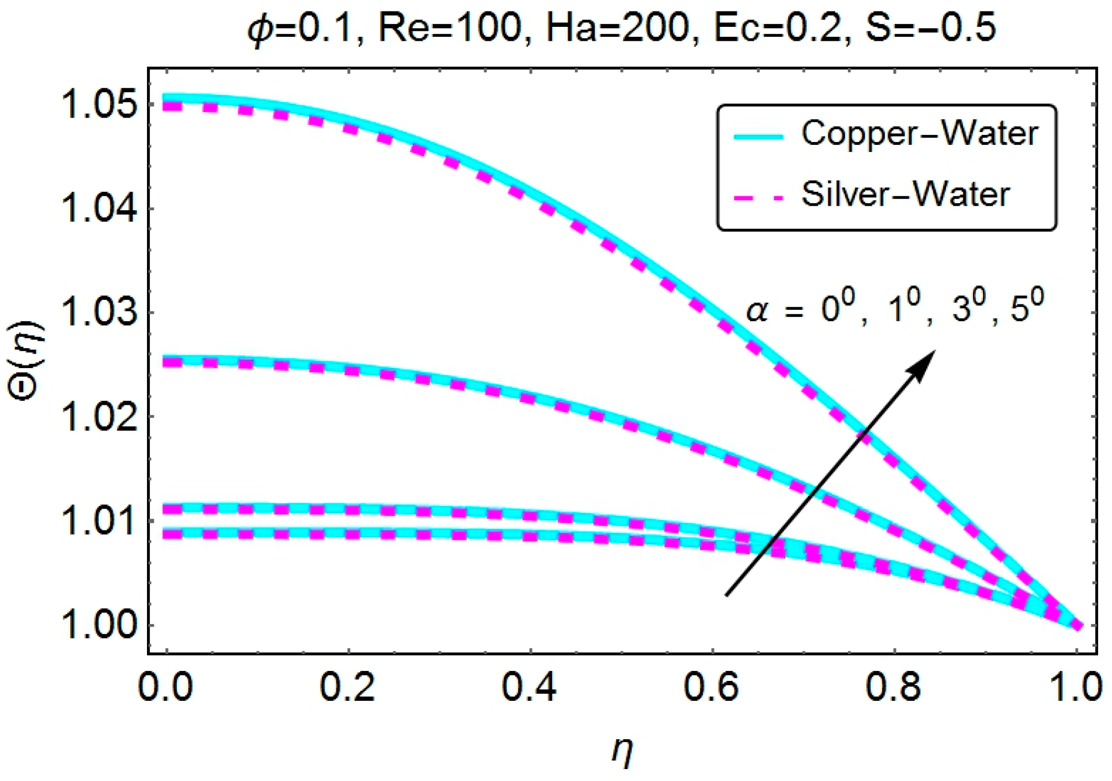
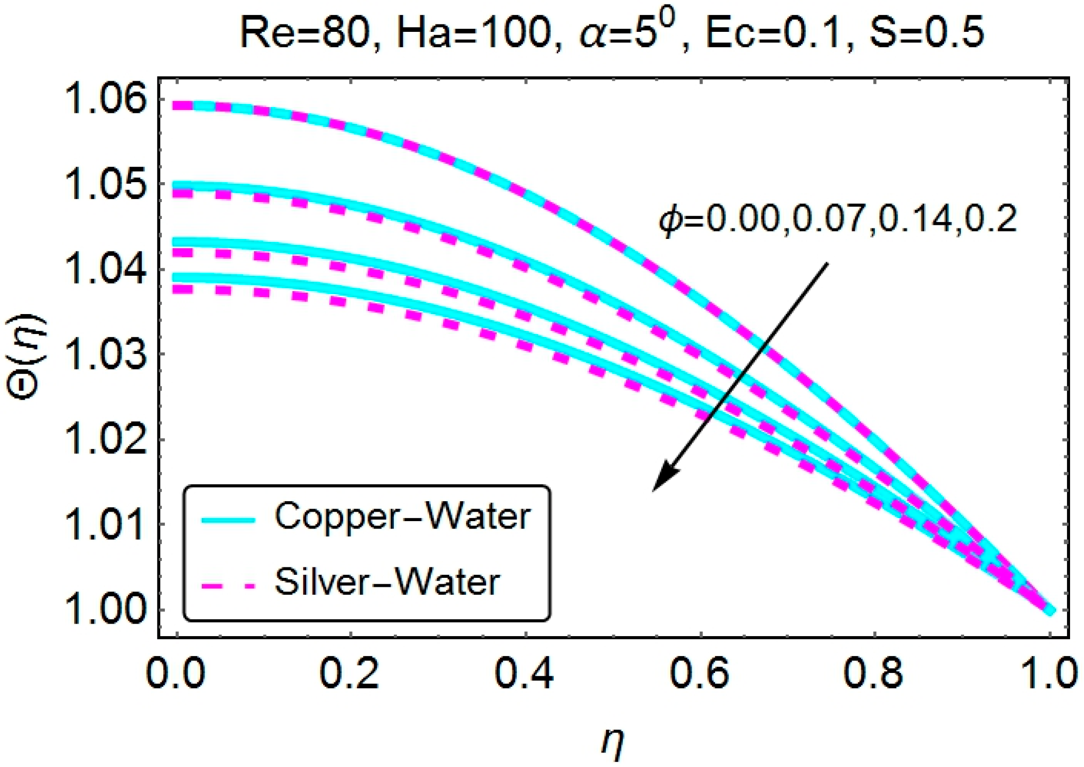
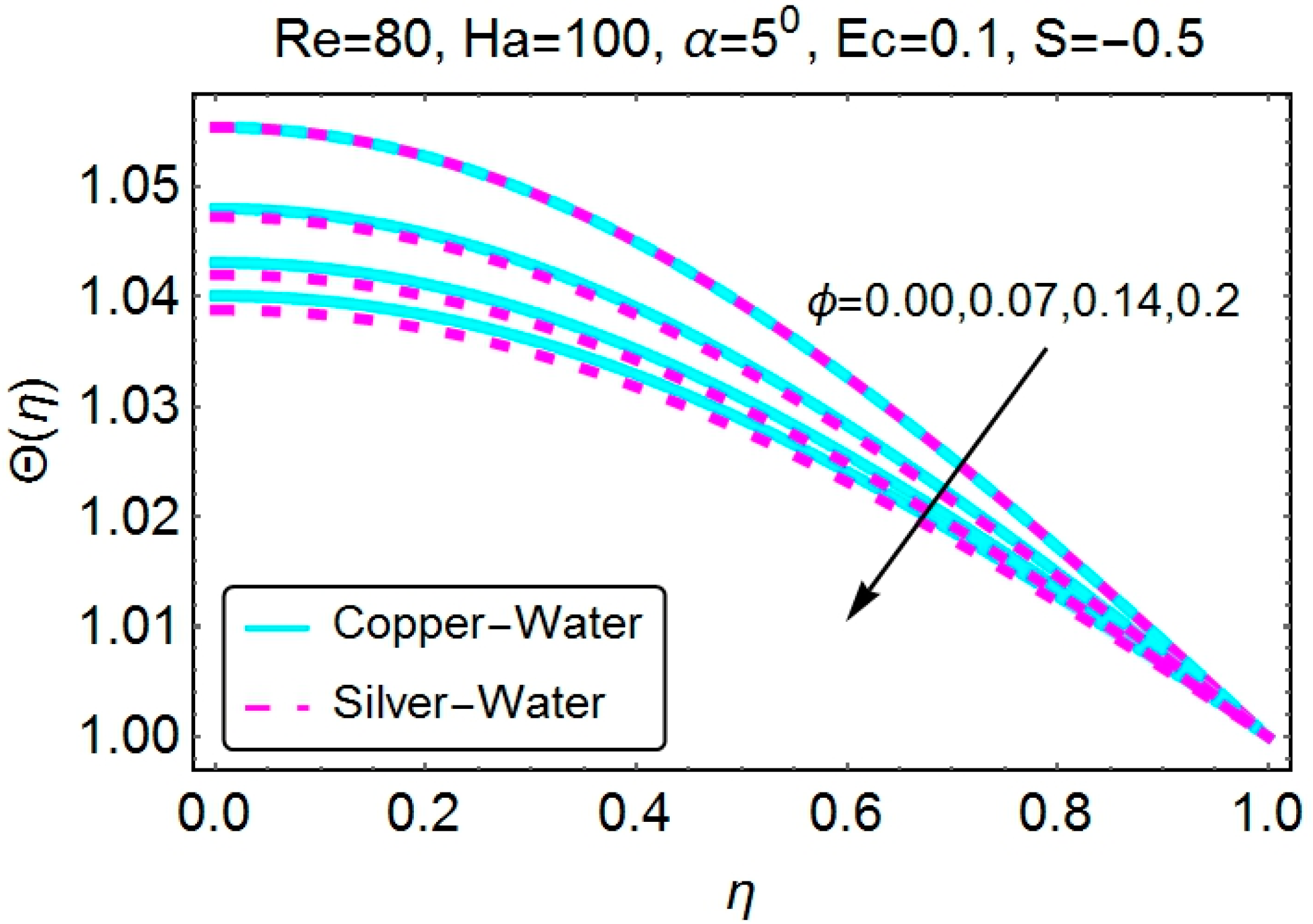
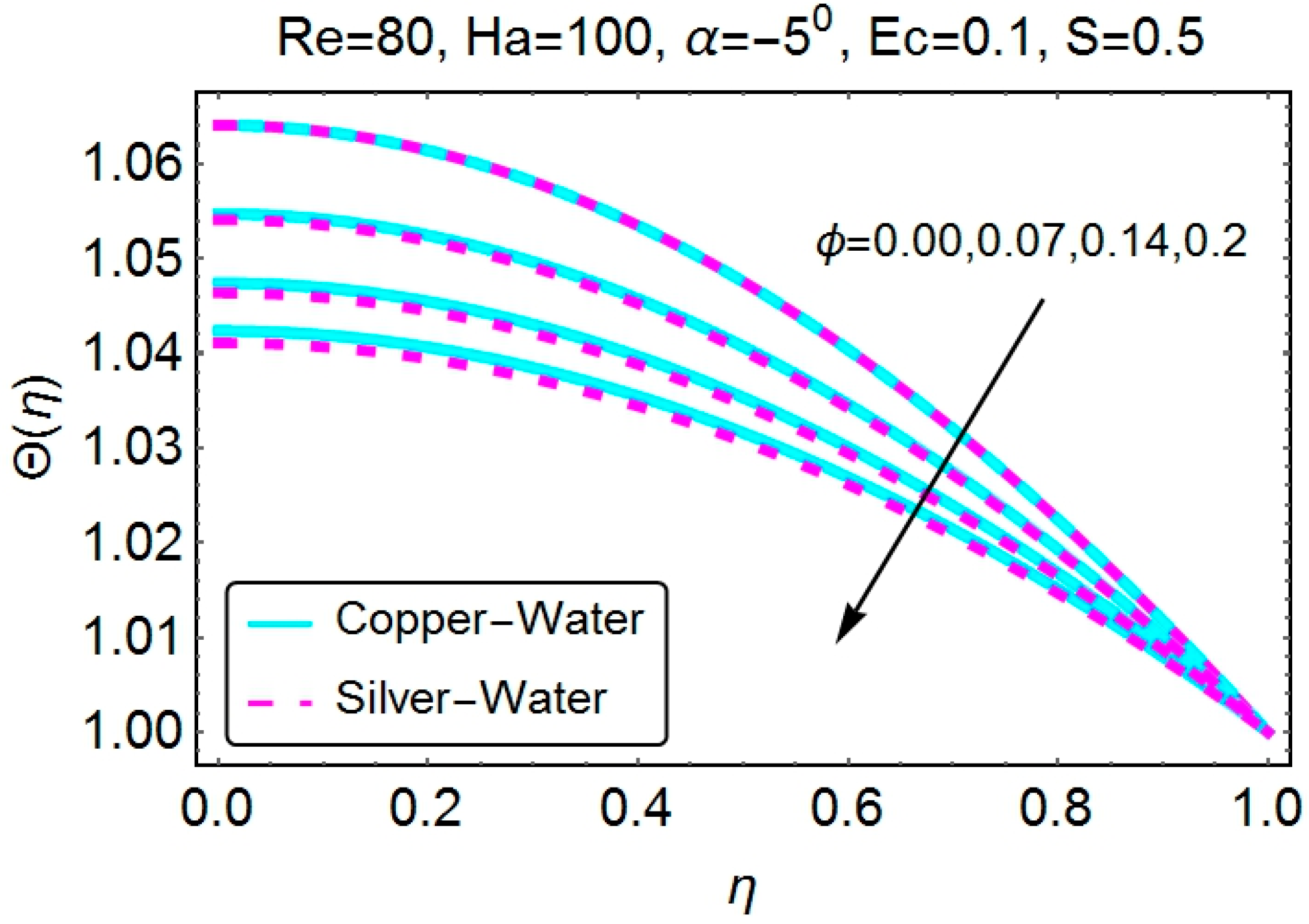
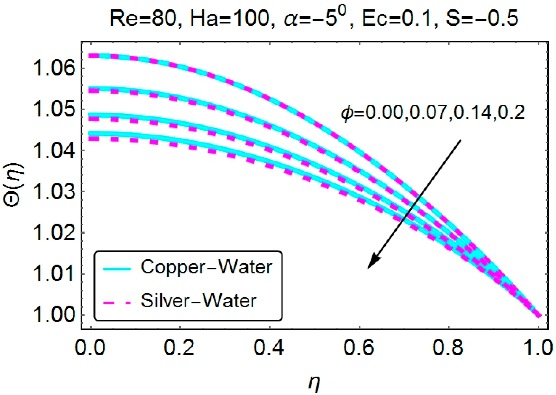
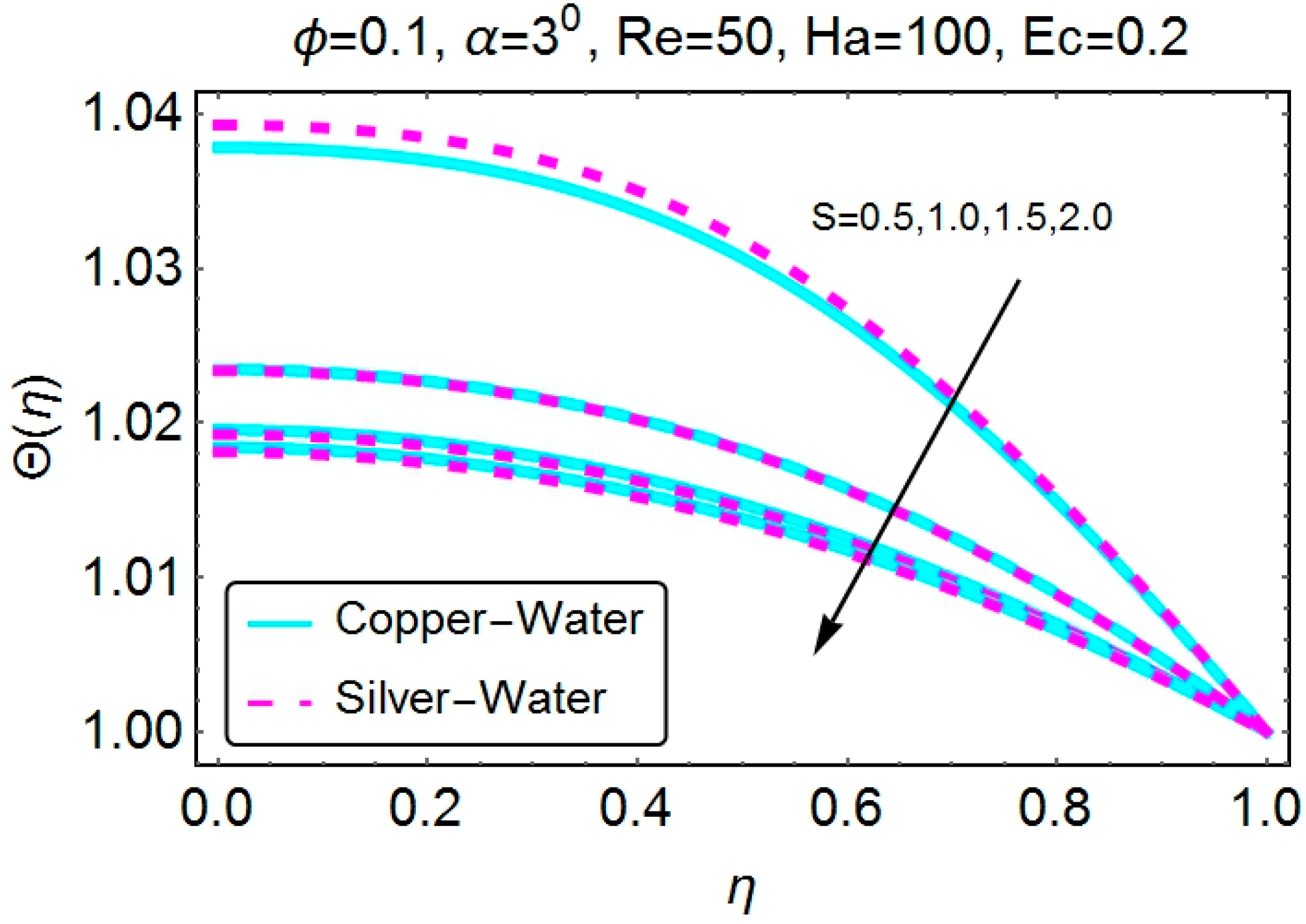
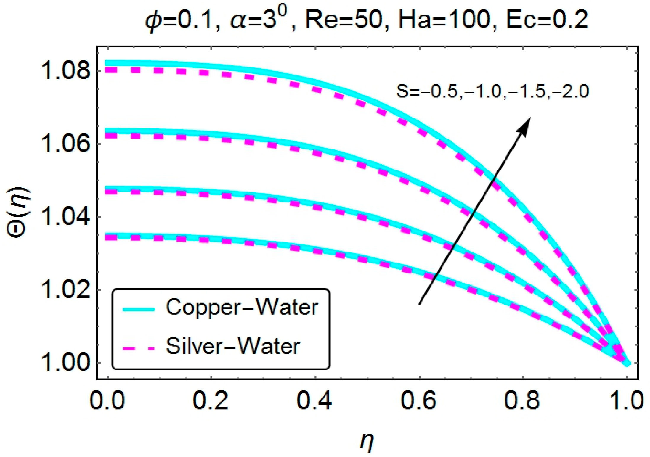
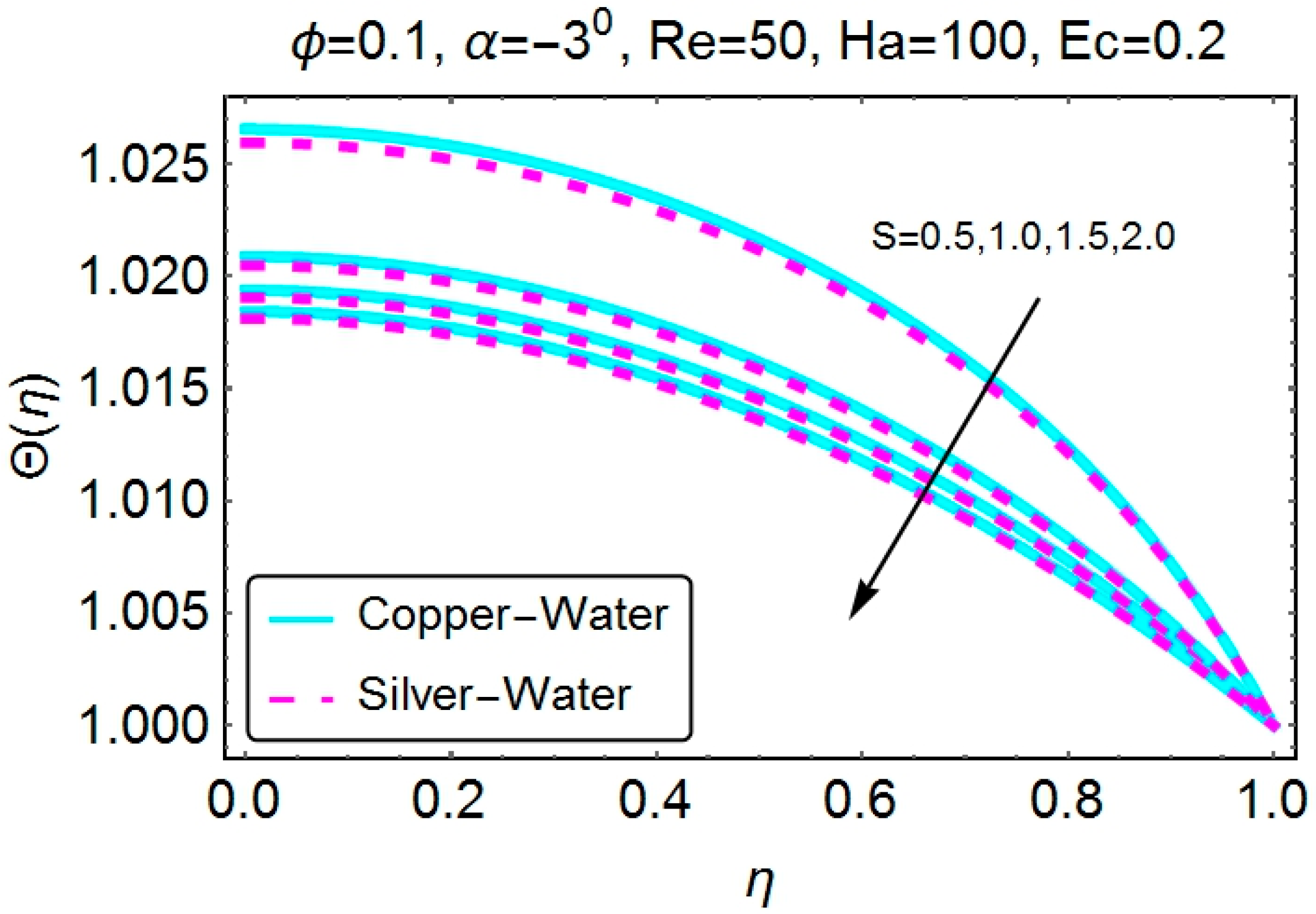
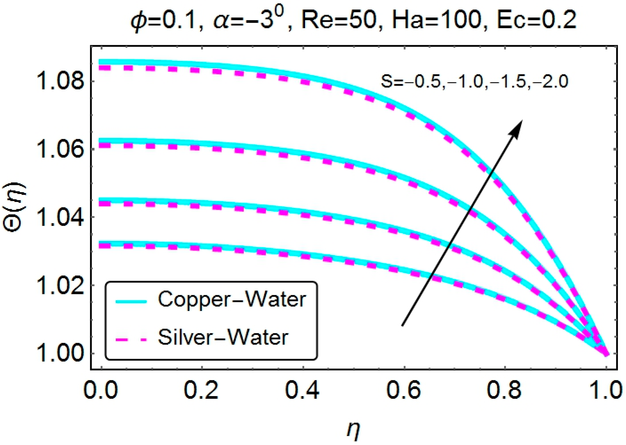
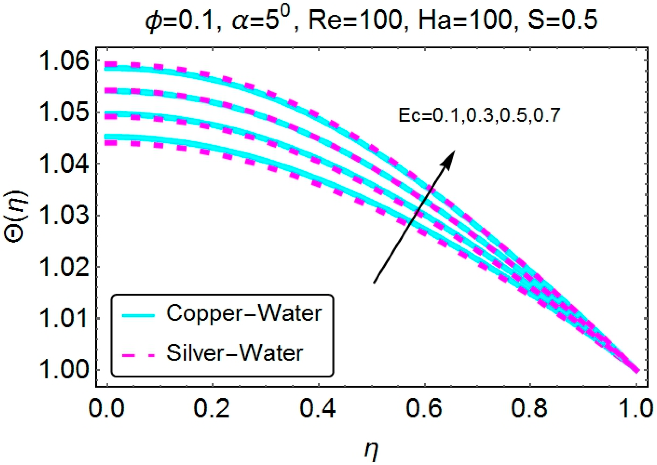
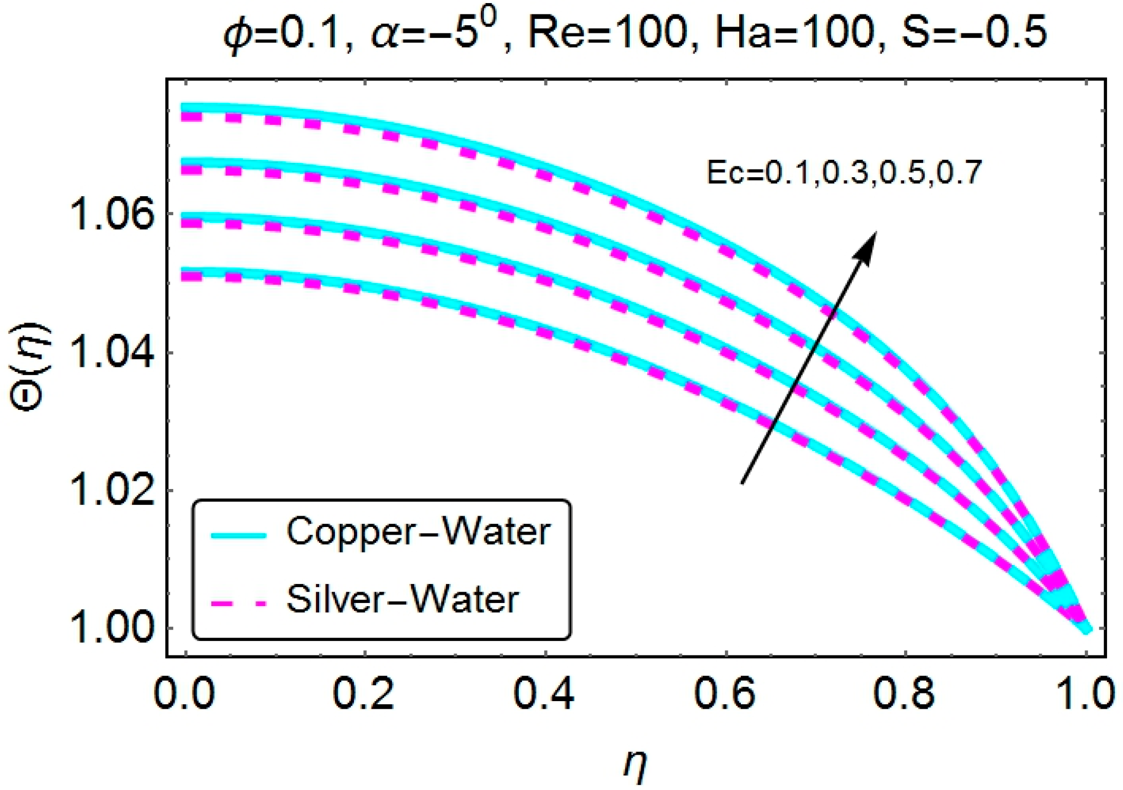
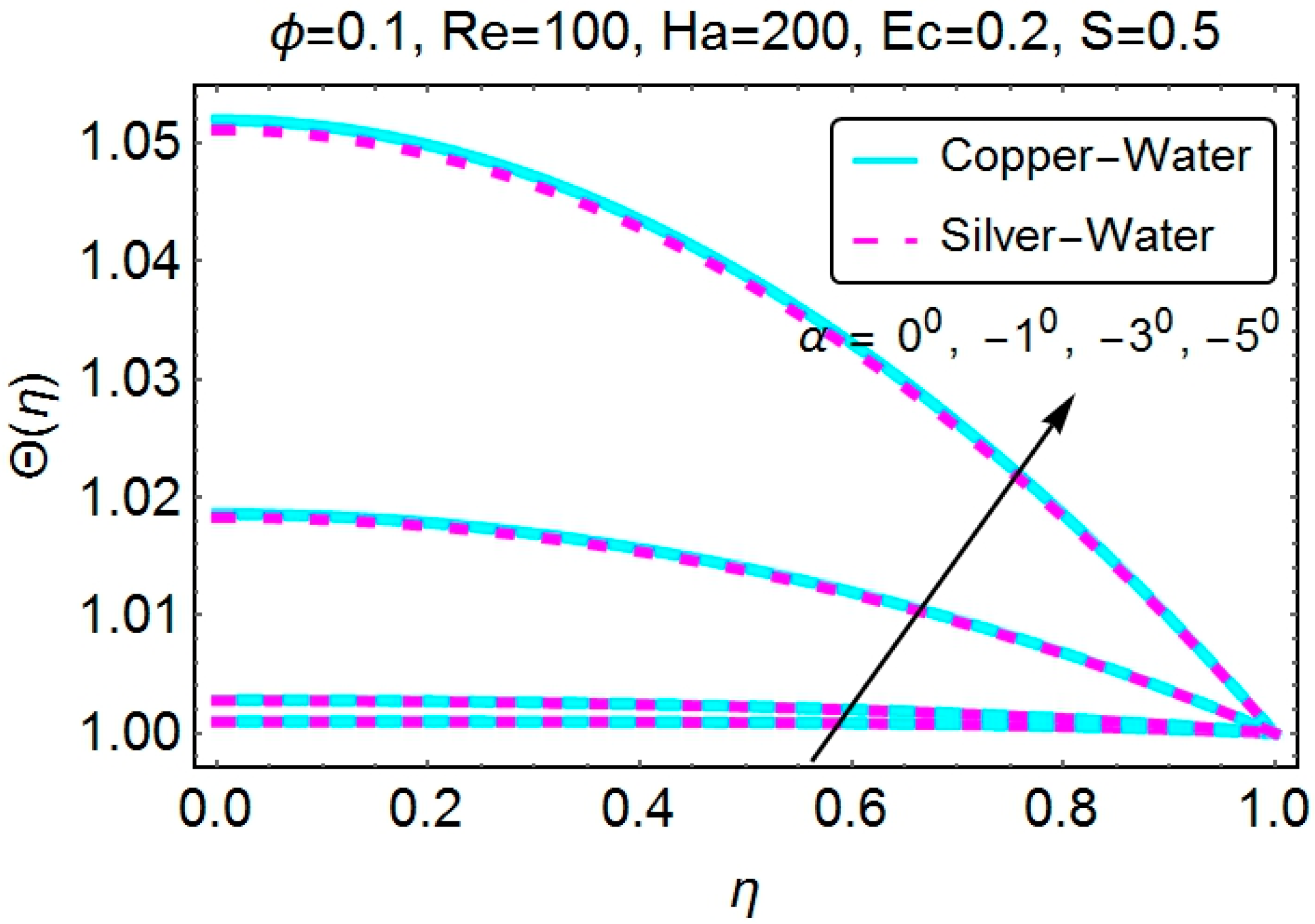
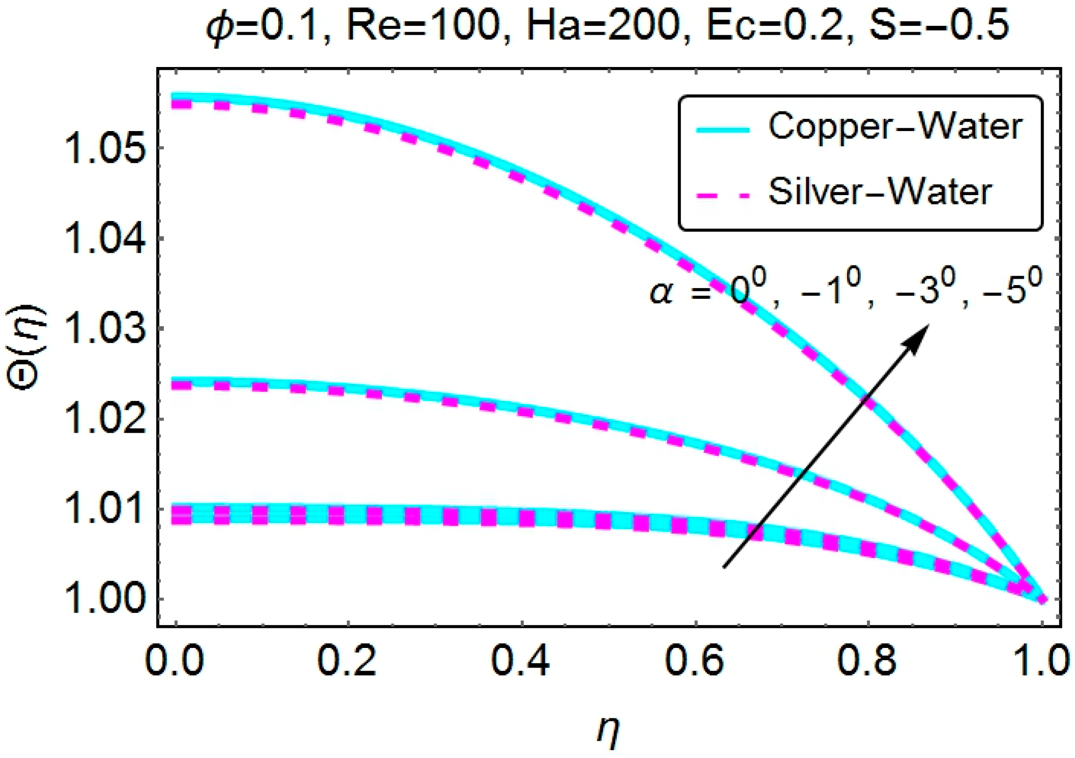
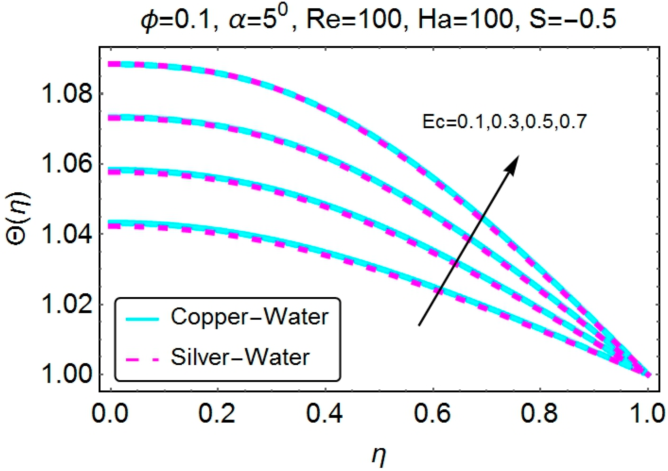
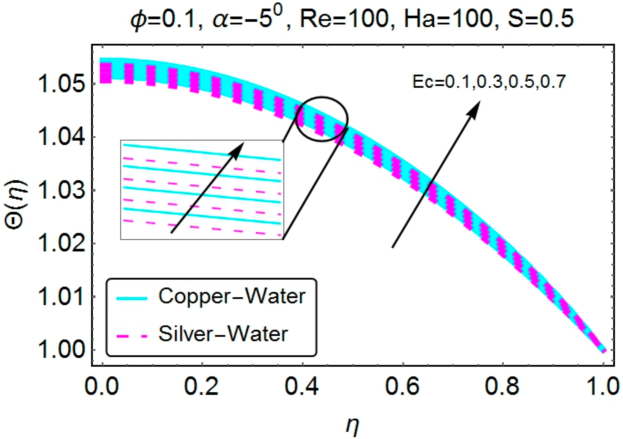
4.2. Temperature Profile

Variations in the temperature profile under the influence of various parameters, like the angle of opening$\mathsf{\text{α}}$, the volume fraction of nanoparticle$\mathsf{\varphi }$, the stretching/shrinking parameter$S$ and the Eckert numbe$Ec$, are plotted in Figure 12, Figure 13, Figure 14, Figure 15, Figure 16, Figure 17, Figure 18, Figure 19, Figure 20, Figure 21, Figure 22, Figure 23, Figure 24, Figure 25, Figure 26 and Figure 27. Here, the value of the Prandtl number$Pr$ is fixed at 6.2 because we are taking water as a base fluid. The temperature profile under the effect of angle opening $\mathsf{\alpha }$ is plotted in Figure 12, Figure 13, Figure 14 and Figure 15. Almost an identical behavior to the temperature profile is observed for both the divergent and convergent channels due to the increasing values of$\mathsf{\text{α}}$. When the walls are stretching, the temperature is seen to be on a slightly lower side for rising$\mathsf{\text{α}}$. On the other hand, for shrinking walls, some higher values of temperature are seen when there is no opening of the walls$\left(\mathsf{\text{α}}=0\right)$. This means whether the walls are stretching or shrinking, with the change in angle, the temperature of the system will rise. There is not much of a difference between the temperature of Cu and Ag.

Figure 12. Change in temperature for varying $\mathsf{\alpha }$ (divergent channel/stretching case).

Figure 12. Change in temperature for varying $\mathsf{\alpha }$ (divergent channel/stretching case).

Figure 13. Change in temperature for varying $\mathsf{\alpha }$ (divergent channel/shrining case).

Figure 13. Change in temperature for varying $\mathsf{\alpha }$ (divergent channel/shrining case).

Figure 14. Change in temperature for varying $\mathsf{\alpha }$ (convergent channel/stretching case).

Figure 14. Change in temperature for varying $\mathsf{\alpha }$ (convergent channel/stretching case).

Figure 15. Change in temperature for varying $\mathsf{\alpha }$ (convergent channel/shrinking case).

Figure 15. Change in temperature for varying $\mathsf{\alpha }$ (convergent channel/shrinking case).

Figure 16. Change in temperature for varying $\mathsf{\phi }$ (divergent channel/stretching case).

Figure 16. Change in temperature for varying $\mathsf{\phi }$ (divergent channel/stretching case).

Figure 17. Change in temperature for varying $\mathsf{\phi }$ (divergent channel/shrinking case).

Figure 17. Change in temperature for varying $\mathsf{\phi }$ (divergent channel/shrinking case).

Figure 18. Change in temperature for varying $\mathsf{\phi }$ (convergent channel/stretching case).

Figure 18. Change in temperature for varying $\mathsf{\phi }$ (convergent channel/stretching case).

Figure 19. Change in temperature for varying $\mathsf{\phi }$ (convergent channel/shrinking case).

Figure 19. Change in temperature for varying $\mathsf{\phi }$ (convergent channel/shrinking case).

Figure 20. Change in temperature for varying $S$ (divergent channel/stretching case).

Figure 20. Change in temperature for varying $S$ (divergent channel/stretching case).

Figure 21. Change in temperature for varying $S$ (divergent channel/shrinking case).

Figure 21. Change in temperature for varying $S$ (divergent channel/shrinking case).

Figure 22. Change in temperature for varying $S$ (convergent channel/stretching case).

Figure 22. Change in temperature for varying $S$ (convergent channel/stretching case).

Figure 23. Change in temperature for varying $S$ (convergent channel/shrinking case).

Figure 23. Change in temperature for varying $S$ (convergent channel/shrinking case).

Figure 24. Change in temperature for varying $Ec$ (divergent channel/stretching case).

Figure 24. Change in temperature for varying $Ec$ (divergent channel/stretching case).

Figure 25. Change in temperature for varying $Ec$ (divergent channel/shrinking case).

Figure 25. Change in temperature for varying $Ec$ (divergent channel/shrinking case).

Figure 26. Change in temperature for varying $Ec$ (convergent channel/stretching case).

Figure 26. Change in temperature for varying $Ec$ (convergent channel/stretching case).

Figure 27. Change in temperature for varying $Ec$ (convergent channel/shrinking case).

Figure 27. Change in temperature for varying $Ec$ (convergent channel/shrinking case).

The influence of the nanoparticle volume fraction on the temperature profile is plotted in Figure 16, Figure 17, Figure 18 and Figure 19. An addition of the nanoparticles in the base fluid decreases the temperature of the system quite considerably. This change is prominent at the centerline of the channel. For a divergent channel, the temperature profile is somewhat on the higher side when the walls are stretching as compared to the shrinking of the walls. For a convergent channel, this behavior is reversed. For all of these cases, silver (Ag) nanoparticles tend to have slightly lower temperature values than copper (Cu) nanoparticles. The differences in the specific heat and the thermal conductivity of Cu and Ag are the major factors for the change in temperature.

The next set of figures describes the behavior of temperature with the stretching/shrinking of the walls. Both the convergent and divergent channel cases are discussed. Figure 20 and Figure 21 depict that the stretching and shrinking of the walls have a quite opposite effect on the temperature profile for a divergent channel. When the walls are stretching, a steep drop in the temperature is observed at the center of the channel. The change becomes smaller as we move near the walls of the channel. On the other hand, the shrinking walls tend to increase the temperature quite substantially at the central portion of the channel. For a convergent channel, the temperature behaves almost in an identical manner as the one seen in a divergent channel; Figure 22 and Figure 23 are here to back our remarks. The only difference is the slightly higher values of the temperature for the stretching walls in a divergent channel. Interestingly, Cu nanoparticles have marginally lower values for the stretching of a divergent channel as compared to the stretching of a convergent channel. For a convergent channel, the temperature of Cu seems to be on the higher side. However, when the walls are shrinking, Cu nanoparticles show a marginal advantage in temperature.

Figure 24, Figure 25, Figure 26 and Figure 27 are plotted to study the changes occurring in the temperature profile due to the variations in$Ec$. Here, Ec represents the influence of dissipation on the temperature profile. As expected, the Eckert number increases the temperature quite expressively. This change in the temperature is slightly lower for the case when the walls are stretching. For the shrinking walls, the temperature rises quite efficiently with increasing values of the Eckert number. Furthermore, for a convergent channel and the stretching walls, the temperature curves deviate relatively less.

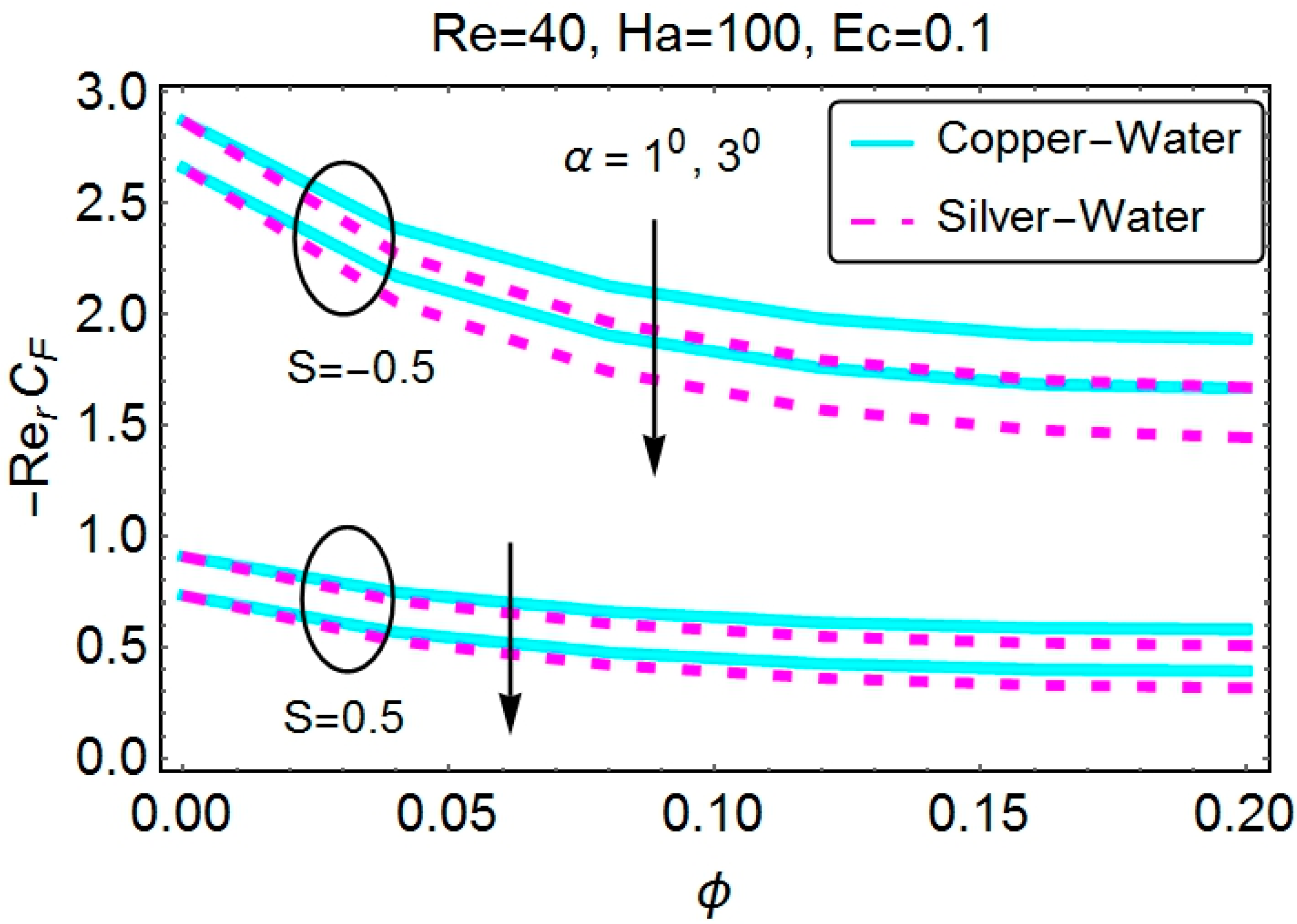
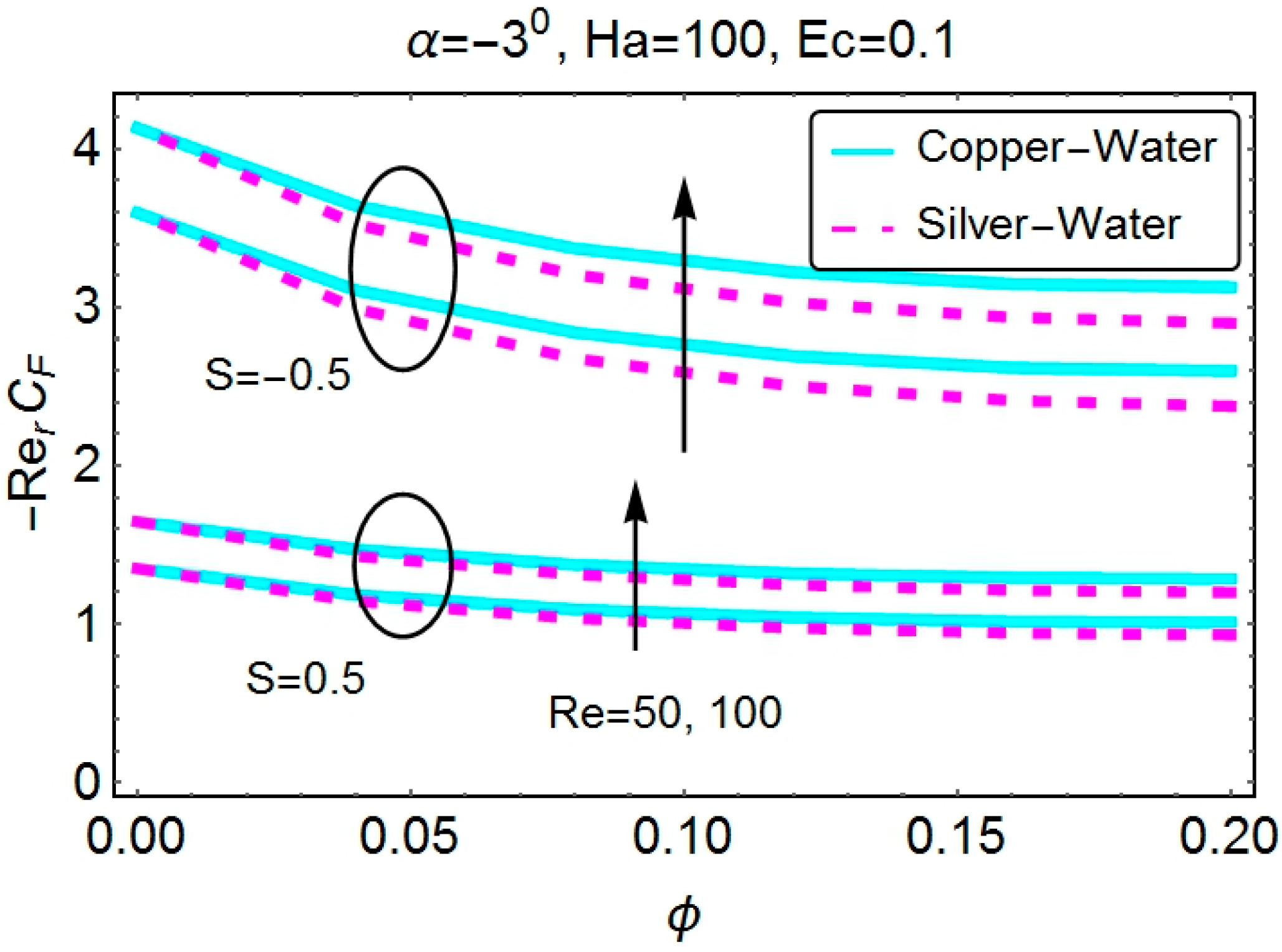
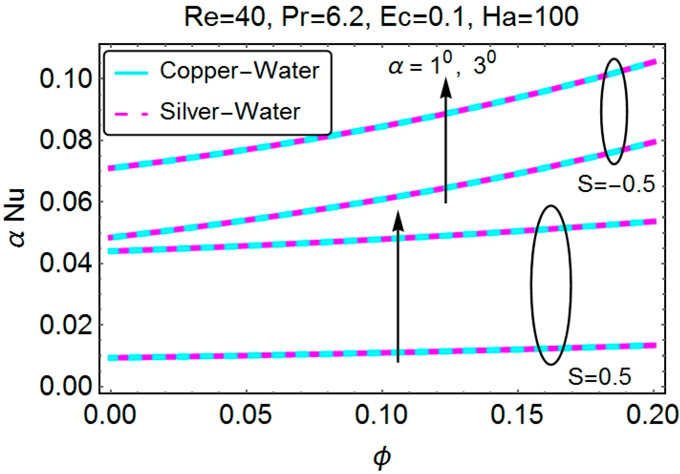
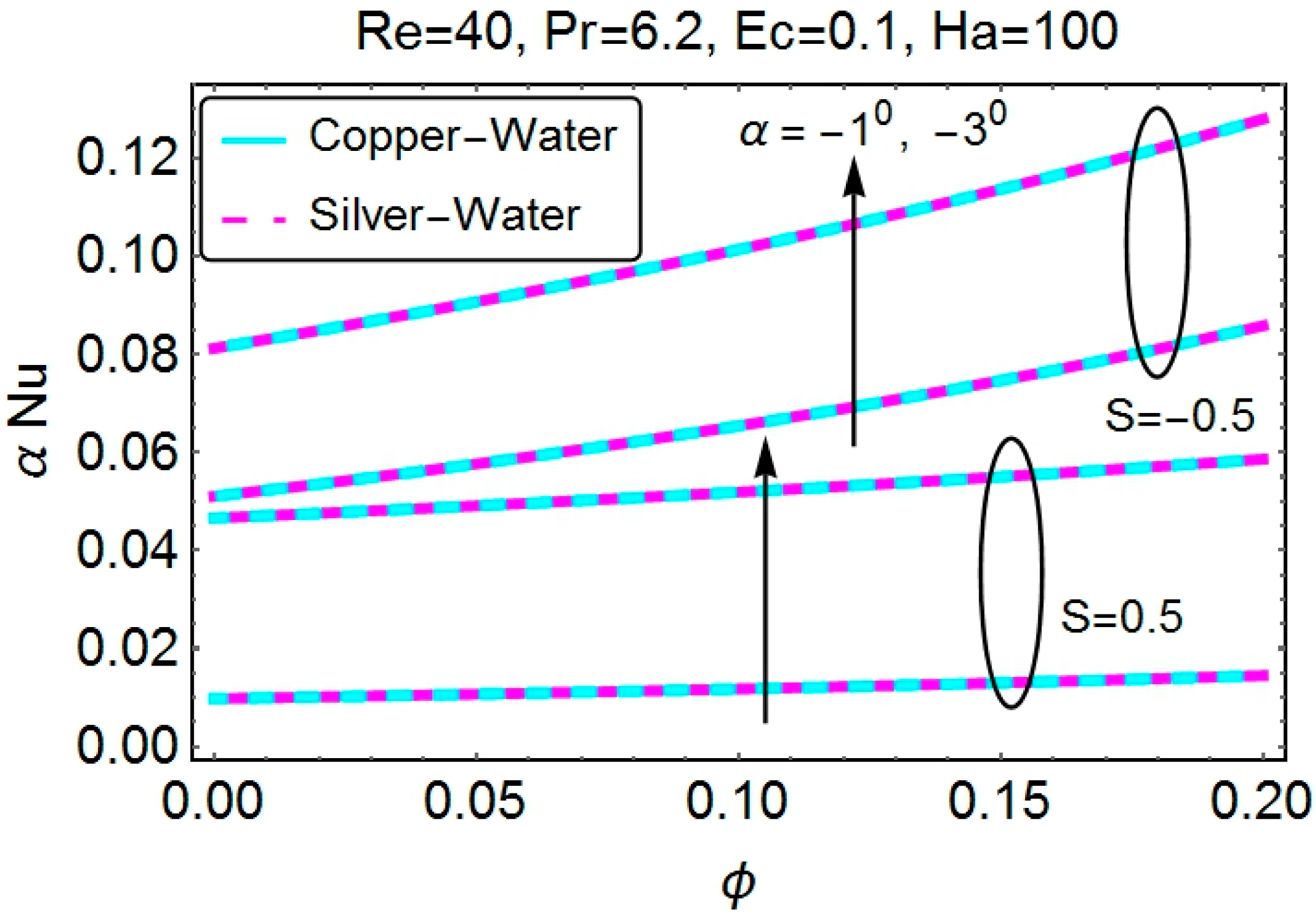
4.3. Skin Friction Coefficient and the Nusselt Number

The effects of various parameters on the skin friction coefficient and the Nusselt number are plotted in Figure 28, Figure 29, Figure 30, Figure 31, Figure 32, Figure 33, Figure 34 and Figure 35. Both stretching and shrinking cases are taken into account. For the case of a divergent channel, Figure 28 gives a description of the varying angle and the nanoparticle volume fraction on the skin friction coefficient. Clearly, with an increase in the nanoparticle volume fraction, the skin friction is seen to be declining for both stretching and shrinking divergent channels. Furthermore, the greater the channel opening for the divergent channel, the lower are the skin friction values. It can be observed that the stretching channel has lower values of the skin friction as compared to the shrinking case. Due to the higher density values, silver nanoparticles have lower values as compared to copper nanoparticles. For the case of the convergent channel, the behavior of the skin friction coefficient can be observed from Figure 29. The skin friction is seen to be increasing with the increase in the angle for the convergent channel. Here, the stretching convergent channel has lower values of the skin friction as compared to the shrinking convergent channel. The manners in which skin friction behaves for increasing values of Re are plotted in Figure 30 and Figure 31. For the divergent channel, the increase in Re results in declining values of the skin friction coefficient, as well as for the nanoparticle volume fraction. Stretching divergent channels have lower skin friction values than shrinking divergent channels. Almost the reverse behavior is observed for the convergent channel, i.e., higher Re values result in higher skin friction values for both stretching and shrinking convergent channels.

Figure 28. Variation in the skin friction coefficient with the angle and the nanoparticle volume fraction (divergent channel).

Figure 28. Variation in the skin friction coefficient with the angle and the nanoparticle volume fraction (divergent channel).

Figure 29. Variation in the skin friction coefficient with the angle and the nanoparticle volume fraction (convergent channel).

Figure 29. Variation in the skin friction coefficient with the angle and the nanoparticle volume fraction (convergent channel).

Figure 30. Variation in the skin friction coefficient with the Reynold number and the nanoparticle volume fraction (divergent channel).

Figure 30. Variation in the skin friction coefficient with the Reynold number and the nanoparticle volume fraction (divergent channel).

Figure 31. Variation in the skin friction coefficient with the Reynold number and the nanoparticle volume fraction (convergent channel).

Figure 31. Variation in the skin friction coefficient with the Reynold number and the nanoparticle volume fraction (convergent channel).

Figure 32. Variation in the Nusselt number with the angle and the nanoparticle volume fraction (divergent channel).

Figure 32. Variation in the Nusselt number with the angle and the nanoparticle volume fraction (divergent channel).

Figure 33. Variation in the Nusselt number with the angle and the nanoparticle volume fraction (convergent channel).

Figure 33. Variation in the Nusselt number with the angle and the nanoparticle volume fraction (convergent channel).

Figure 34. Variation in the Nusselt number with the Eckert number and the nanoparticle volume fraction (divergent channel).

Figure 34. Variation in the Nusselt number with the Eckert number and the nanoparticle volume fraction (divergent channel).

Figure 35. Variation in the Nusselt number with the Eckert number and the nanoparticle volume fraction (convergent channel).

Figure 35. Variation in the Nusselt number with the Eckert number and the nanoparticle volume fraction (convergent channel).

Changes in the Nusselt number with varying parameters are plotted in Figure 32, Figure 33, Figure 34 and Figure 35 both for divergent and convergent channels. Figure 32 gives a description of the change in the Nusselt number with the varying nanoparticle volume fraction and the angle for the divergent channel case. The heat transfer rate at the wall is seen to be an increasing function of both the angle and the nanoparticle volume fraction. This behavior is quite fast for a shrinking divergent channel. A similar pattern is seen for the convergent channel, the difference being only that, for the convergent channel case, the values are slightly on the higher side as compared to the same values for the divergent channel, as depicted in Figure 33. Apparently, there is no difference in the values for copper and silver nanoparticles. The increase in the Eckert number results in a higher heat transfer rate at the wall for both divergent and convergent channels. The stretching of walls has a dominant effect as compared to the shrinking of the walls. The nanoparticle volume fraction increases the heat transfer rate and, thus, can be useful in many industrial processes. The problem under consideration is solved using two methods: the variational iteration method and the Runge-Kutta-Fehlberg method. The results obtained are compared to existing solutions when there is no magnetic field and the fluid is taken as water only. An excellent agreement between the solutions is seen, as given in Table 2 and Table 3.

Table 2. Comparison of the numerical values for the skin friction coefficient with the already existing solutions in the literature for $\mathrm{Re}=50, Ha=0, \mathsf{\phi }=0.$ VIM, variational iteration method; RKF, Runge–Kutta–Fehlberg method.

S	$F\prime \left(1\right)(\mathsf{\alpha }=5^{°})$			S	$F\prime \left(1\right)(\mathsf{\alpha }=-5^{°})$
↓	VIM	RKF	Turkyilmazoglu [38]	↓	VIM	RKF	Turkyilmazoglu [38]
−1	−3.508103	−3.508103	−3.508103	−2	−5.130922	−5.130922	−5.130922
−1/2	−2.173044	−2.173044	−2.173044	−1	−4.652159	−4.652159	−4.652159
0	0.000000	0.000000	0.000000	0	−2.833951	−2.833951	−2.833951
1/2	−0.361846	−0.361846	−0.361846	1	0.000000	0.000000	0.000000
1	0.000000	0.000000	0.000000	2	3.669711	3.669711	3.669711

Table 2. Comparison of the numerical values for the skin friction coefficient with the already existing solutions in the literature for $\mathrm{Re}=50, Ha=0, \mathsf{\phi }=0.$ VIM, variational iteration method; RKF, Runge–Kutta–Fehlberg method.

S	$F\prime \left(1\right)(\mathsf{\alpha }=5^{°})$			S	$F\prime \left(1\right)(\mathsf{\alpha }=-5^{°})$
↓	VIM	RKF	Turkyilmazoglu [38]	↓	VIM	RKF	Turkyilmazoglu [38]
−1	−3.508103	−3.508103	−3.508103	−2	−5.130922	−5.130922	−5.130922
−1/2	−2.173044	−2.173044	−2.173044	−1	−4.652159	−4.652159	−4.652159
0	0.000000	0.000000	0.000000	0	−2.833951	−2.833951	−2.833951
1/2	−0.361846	−0.361846	−0.361846	1	0.000000	0.000000	0.000000
1	0.000000	0.000000	0.000000	2	3.669711	3.669711	3.669711

Table 3. Comparison of the numerical values for the Nusselt number with the already existing solutions in the literature for $\mathrm{Re}=50,Ha=0,\mathsf{\phi }=0.$

S	$\mathbf{-}\mathrm{\Theta }\prime \mathbf{\left(}\mathbf{1}\mathbf{\right)}(\mathsf{\alpha }=5^{°})$			S	$\mathbf{-}\mathrm{\Theta }\prime \mathbf{\left(}\mathbf{1}\mathbf{\right)}(\mathsf{\alpha }=-5^{°})$
↓	VIM	RKF	Turkyilmazoglu [38]	↓	VIM	RKF	Turkyilmazoglu [38]
−1	0.034775	0.034775	0.034775	−2	0.031576	0.031576	0.031576
−1/2	0.0372685	0.0372685	0.0372685	−1	0.037322	0.037322	0.037322
0	0.039982	0.039982	0.039982	0	0.042151	0.042151	0.042151
1/2	0.042986	0.042986	0.042986	1	0.046401	0.046401	0.046401
1	0.046401	0.046401	0.046401	2	0.050242	0.050242	0.050242

Table 3. Comparison of the numerical values for the Nusselt number with the already existing solutions in the literature for $\mathrm{Re}=50,Ha=0,\mathsf{\phi }=0.$

S	$\mathbf{-}\mathrm{\Theta }\prime \mathbf{\left(}\mathbf{1}\mathbf{\right)}(\mathsf{\alpha }=5^{°})$			S	$\mathbf{-}\mathrm{\Theta }\prime \mathbf{\left(}\mathbf{1}\mathbf{\right)}(\mathsf{\alpha }=-5^{°})$
↓	VIM	RKF	Turkyilmazoglu [38]	↓	VIM	RKF	Turkyilmazoglu [38]
−1	0.034775	0.034775	0.034775	−2	0.031576	0.031576	0.031576
−1/2	0.0372685	0.0372685	0.0372685	−1	0.037322	0.037322	0.037322
0	0.039982	0.039982	0.039982	0	0.042151	0.042151	0.042151
1/2	0.042986	0.042986	0.042986	1	0.046401	0.046401	0.046401
1	0.046401	0.046401	0.046401	2	0.050242	0.050242	0.050242

5. Conclusions

This article is presented to study the flow and heat transfer of water-based nanofluids in stretchable convergent/divergent channels. The magnetohydrodynamic nature of the flow is incorporated. Copper and silver nanoparticles are added to water to analyze the behavior of the velocity and temperature profiles with varying the parameters involved. Equations governing the flow are solved using two methods, namely VIM and RK-F. A comparison with existing solutions is also given to check the accuracy of our obtained results. The effects of the parameters on the skin friction coefficient and heat transfer at the wall are also plotted. The major outcomes of this study are as follows:

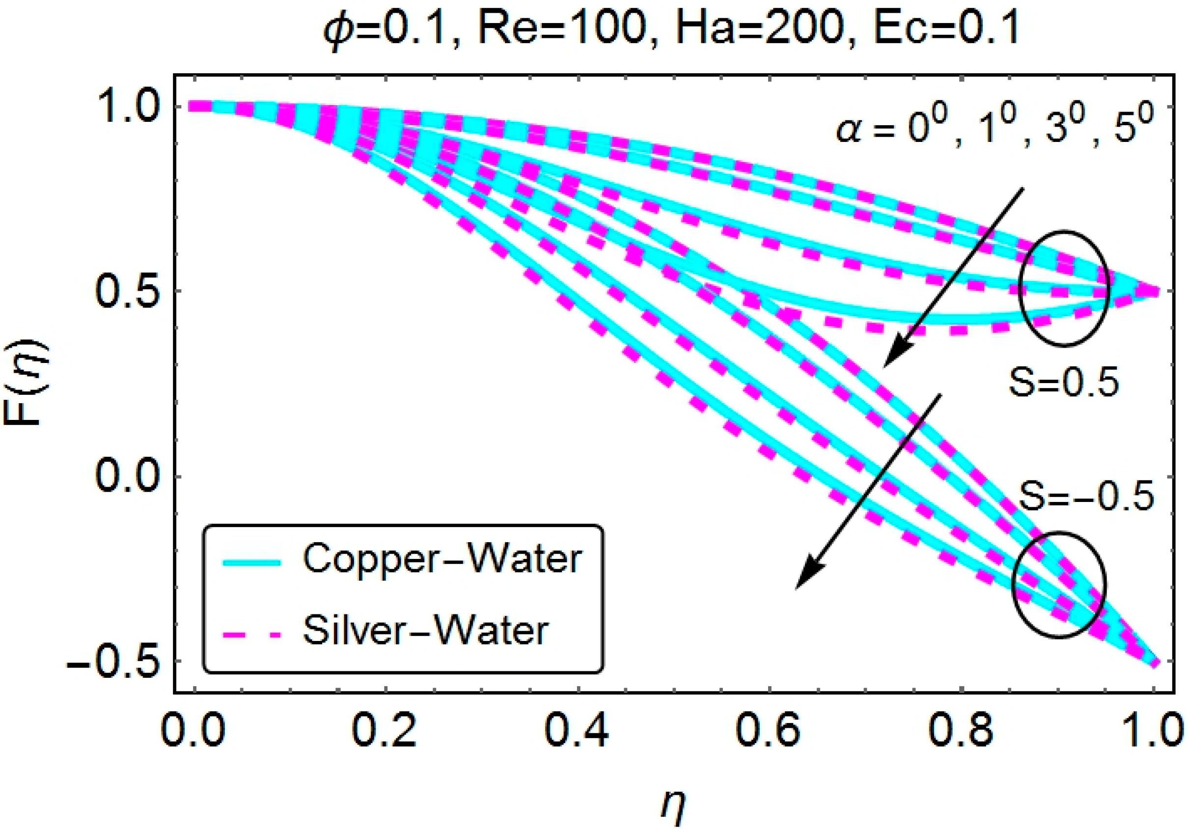
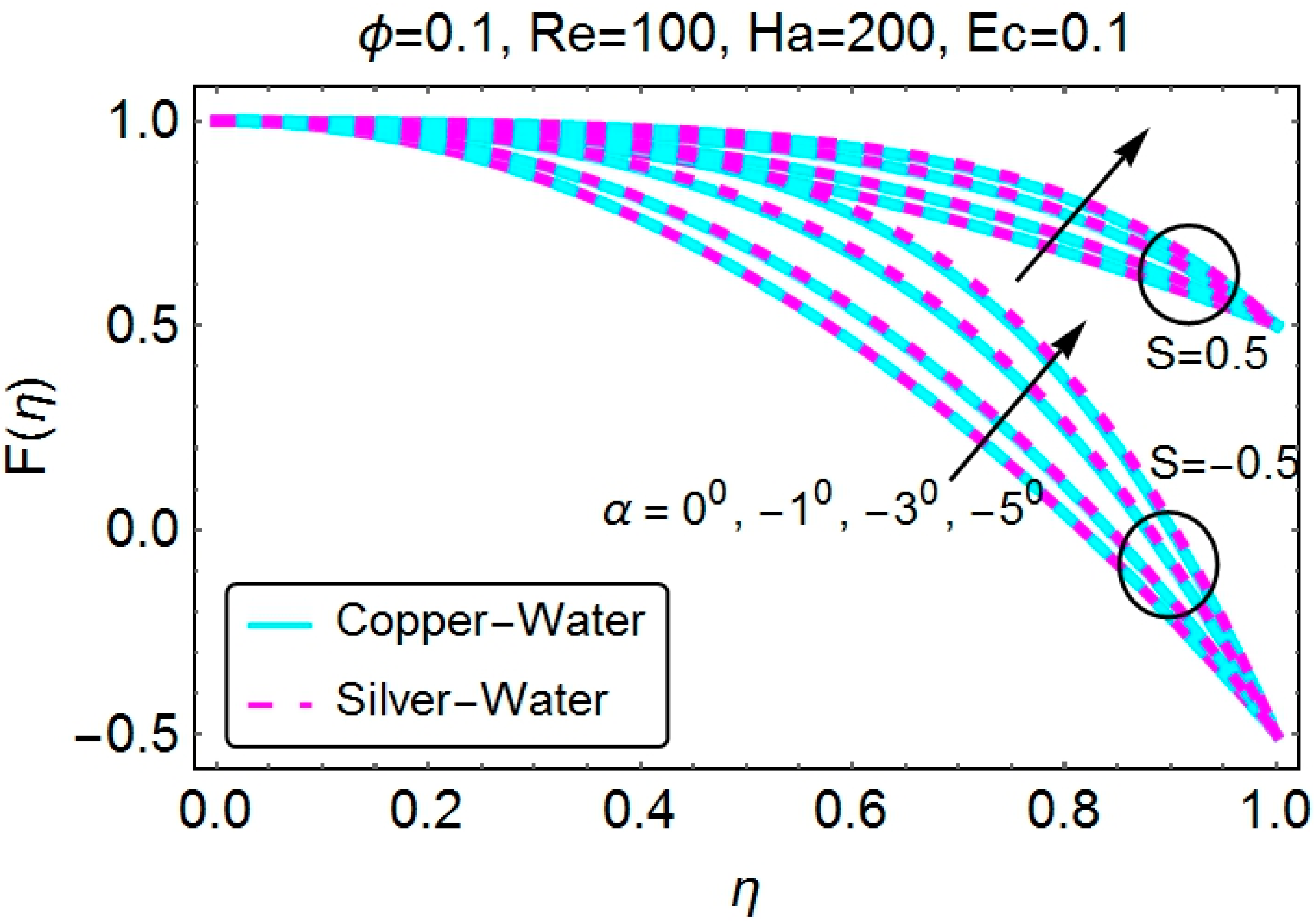
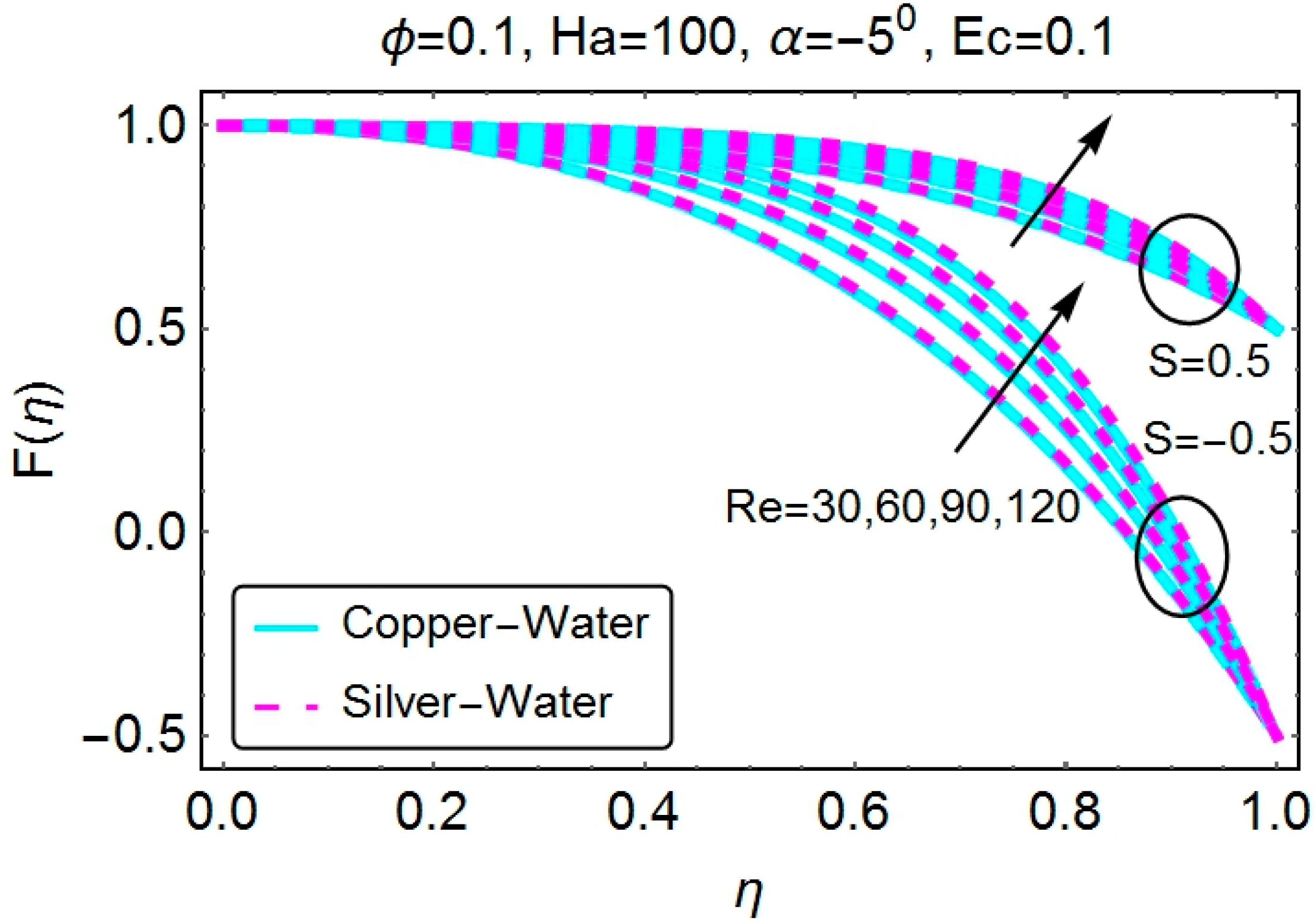
• Angle opening and the Reynolds number have opposite effects on the velocity profile for convergent and divergent channels.
• Stretching walls may result in backflow regimes for divergent channels, because this moves the particles near the wall away. An increase in the angle opening and Reynolds number may result in backflow and, thus, separation. This result might cause instabilities in the flow.
• The Hartmann number gives a solution to the backflow regions. An increase in the Hartmann number removes the backflow for stretching divergent channels. This effect can be useful in several physical phenomena.
• The nanoparticle volume fraction reduces the velocity of the fluid for both copper and silver nanoparticles in the case of a divergent channel. For a convergent channel, the increase in the volume fraction increases the velocity.
• Stretching of the divergent channel increases the flow near the walls of the channel. Additionally, shrinking reduces the velocity of the fluid near the walls of the channel. Identical behavior is seen for the case of a convergent channel.
• The almost identical behavior of the temperature profile for increasing channel opening is observed for both convergent and divergent channels, both for stretching and shrinking channels.
• Temperature is seen to be decreasing for increasing values of the nanoparticle volume fraction. Both stretching and shrinking channels have an almost identical behavior.
• Stretching of the walls results in lower temperature values for both convergent and divergent channels. Increasing values of temperature near the walls of the channel are observed for the shrinking case.
• The Eckert number increases the temperature of the fluid for all of the cases.
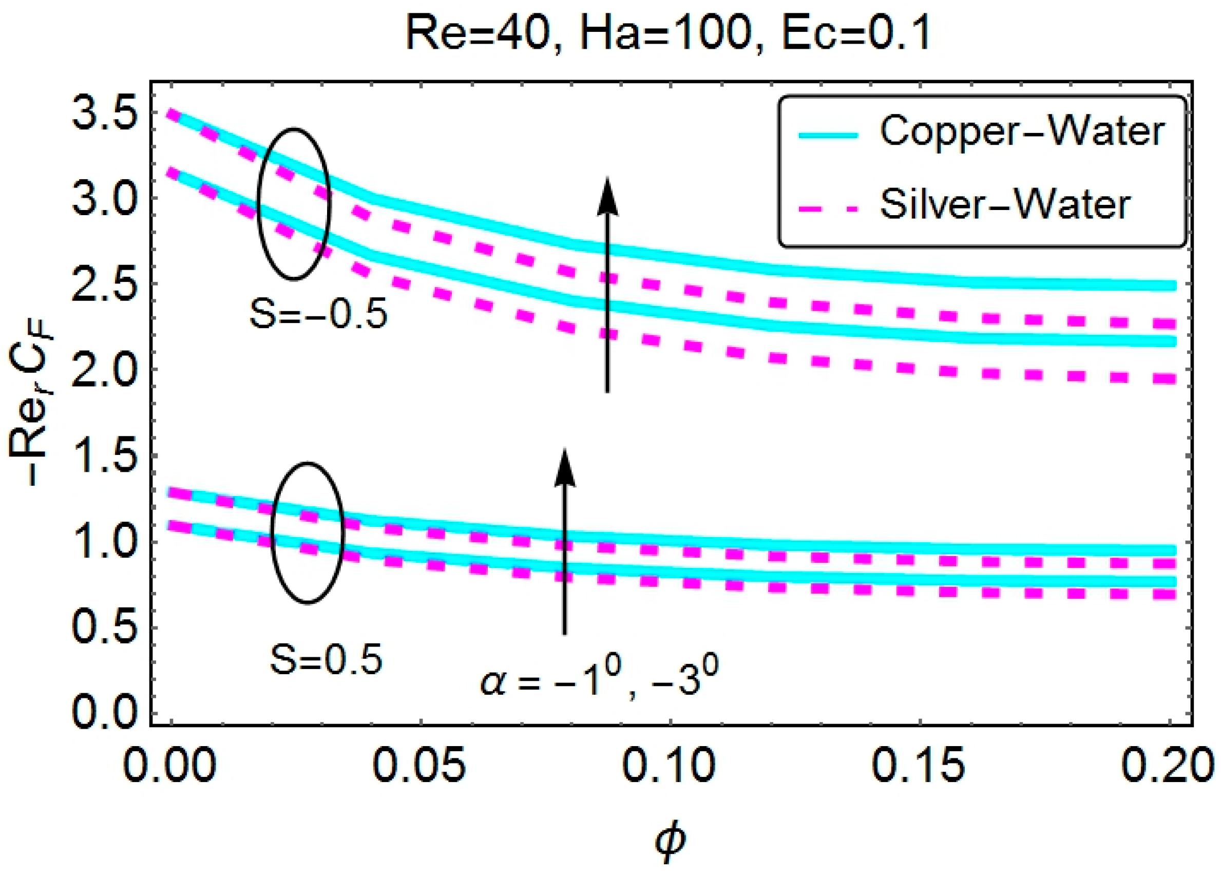
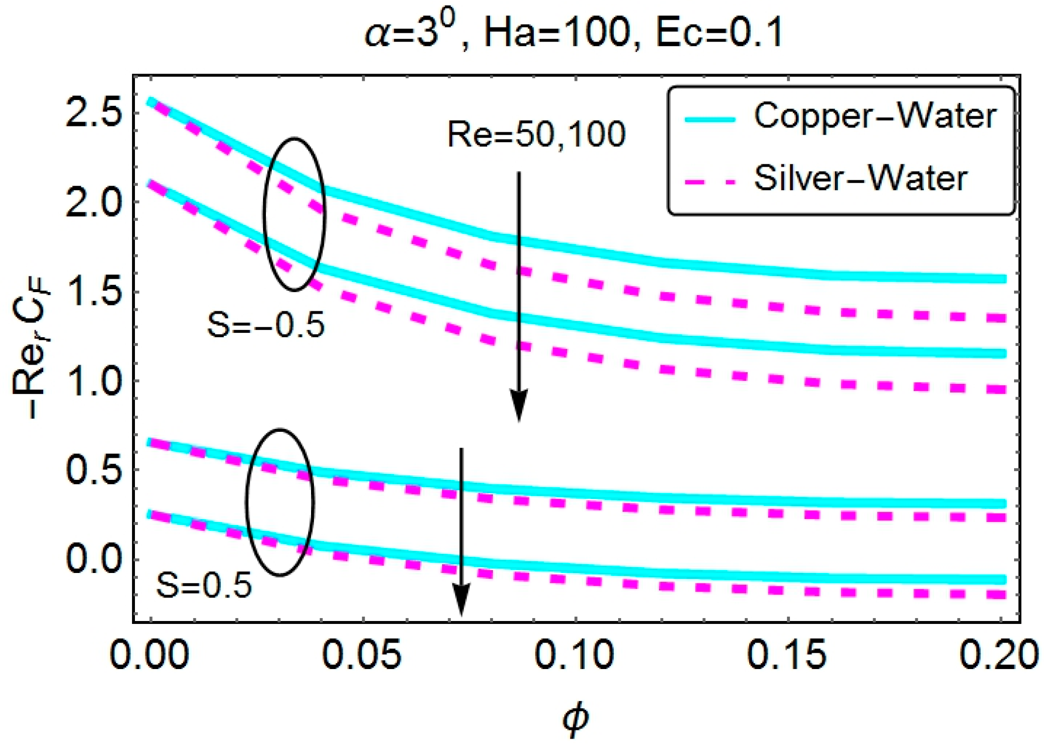
• The nanoparticle volume fraction reduces the skin friction coefficient for all of the cases. Stretching channels have lower skin friction values than shrinking channels.
• The opposite behavior of the skin friction coefficient for increasing Re is observed for convergent and divergent channels.
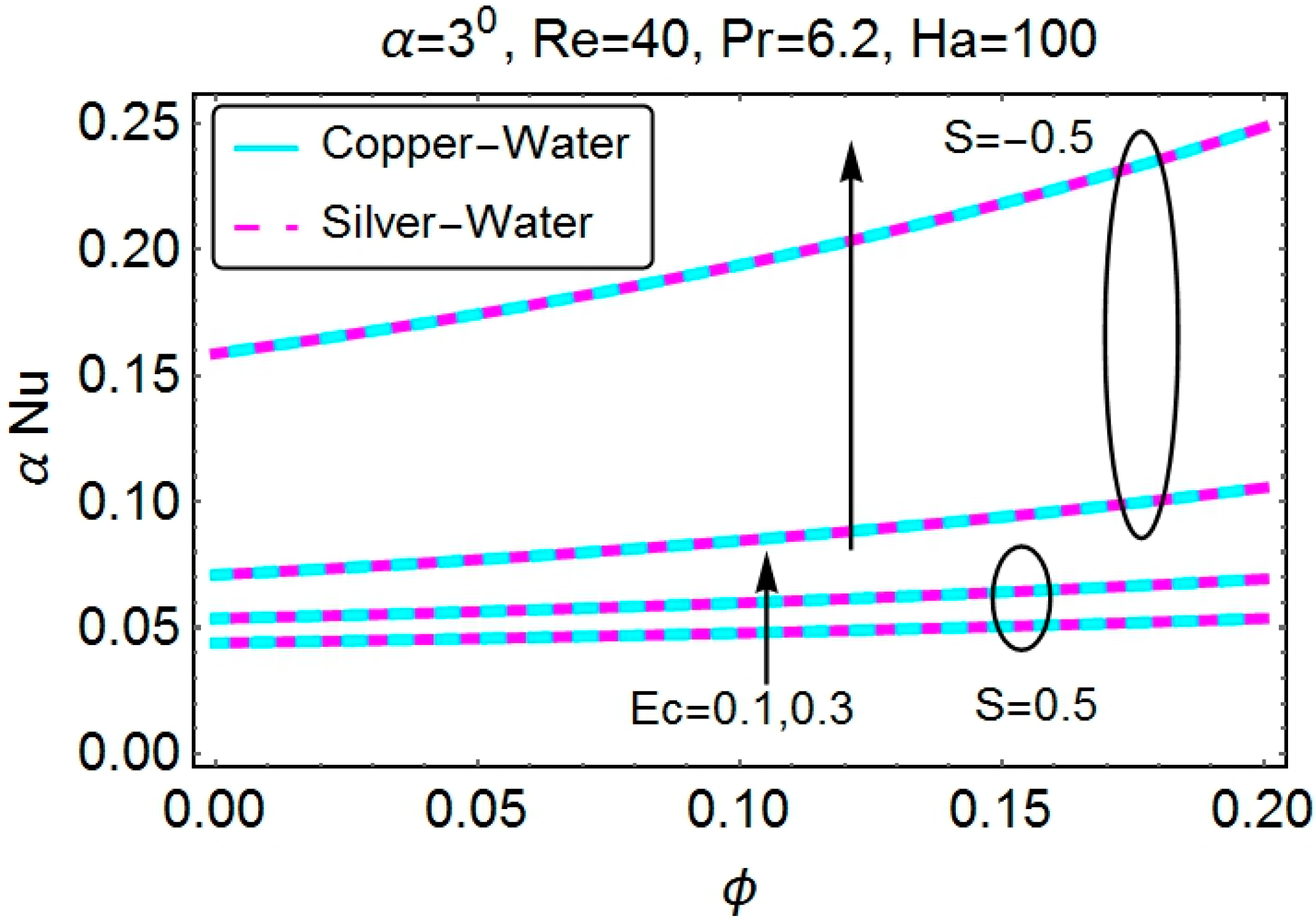
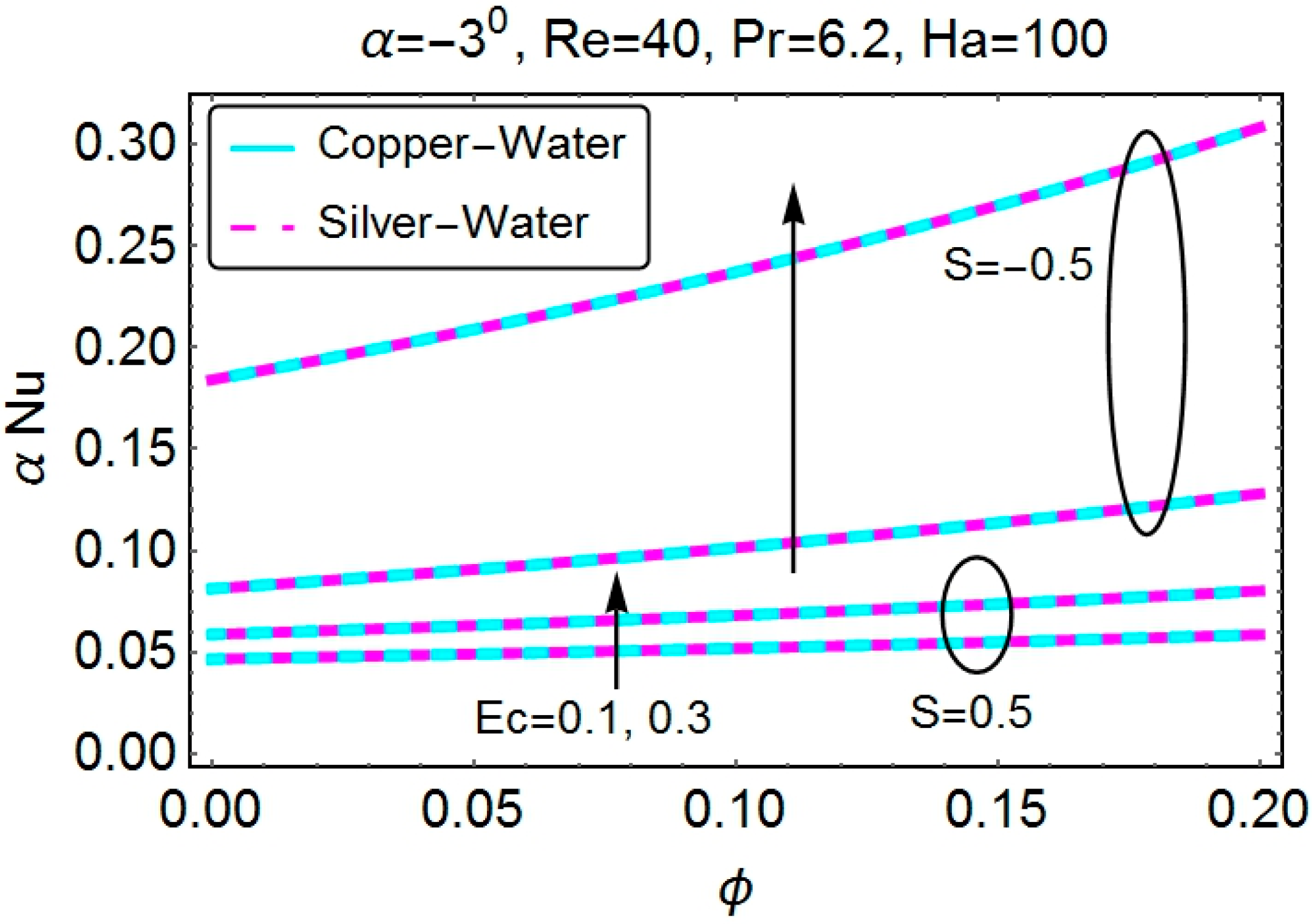
• The rate of heat transfer at the wall increases with a higher nanoparticle volume fraction and Eckert number. These two parameters have the same behavior for all of the cases.

References

1. Jeffery, G.B. The two-dimensional steady motion of a viscous fluid. Philos. Mag. 1915, 6, 455–465. [Google Scholar] [CrossRef]
2. Hamel, G. Spiralförmige Bewgungen ZäherFlüssigkeiten. Jahresber. Deutsch. Math. Verein. 1916, 25, 34–60. [Google Scholar]
3. Asadullah, M.; Khan, U.; Ahmed, N.; Manzoor, R.; Mohyud-Din, S.T. MHD Flow of a Jeffery Fluid in Converging and Diverging Channels. Int. J. Mod. Math. Sci. 2013, 6, 92–106. [Google Scholar]
4. Motsa, S.S.; Sibanda, P.; Marewo, G.T. On a new analytical method for flow between two inclined walls. Numer. Algorithms 2012, 61, 499–514. [Google Scholar] [CrossRef]
5. Crane, L.J. Flow past a stretching plate. Z. Angew. Math. Phys. 1970, 21, 645–647. [Google Scholar] [CrossRef]
6. Akbar, N.S.; Nadeem, S.; Haq, R.U.; Khan, Z.H. Radiation effects on MHD stagnation point flow of nano fluid towards a stretching surface with convective boundary condition. Chin. J. Aeronaut. 2013, 26, 1389–1397. [Google Scholar] [CrossRef]
7. Nadeem, S.; Haq, R.U. Effect of Thermal Radiation for Megnetohydrodynamic Boundary Layer Flow of a Nanofluid Past a Stretching Sheet with Convective Boundary Conditions. J. Comput. Theor. Nanosci. 2013, 11, 32–40. [Google Scholar] [CrossRef]
8. Magyari, E.; Keller, B. Exact solutions for self-similarboundary-layerflows induced by permeable stretching walls. Eur. J. Mech. B Fluids 2000, 19, 109–122. [Google Scholar] [CrossRef]
9. Choi, S.U.S.; Eastman, J.A. Enhancing thermal conductivity of fluids with nanoparticle. In Proceedings of ASME International Mechanical Engineering Congress & Exposition, San Francisco, CA, USA, 12–17 November 1995.
10. Choi, S.U.S.; Zhang, Z.G.; Yu, W.; Lockwood, F.E.; Grulke, E.A. Anomalously thermal conductivity enhancement in nanotube suspensions. Appl. Phys. Lett. 2001, 79, 2252–2254. [Google Scholar] [CrossRef]
11. Buongiorno, J. Convective transport in nanofluids. ASME J. Heat Transf. 2006, 128, 240–250. [Google Scholar] [CrossRef]
12. Xue, Q. Model for thermal conductivity of carbon nanotube-based composites. Phys. B Condens. Matter 2005, 368, 302–307. [Google Scholar] [CrossRef]
13. Hamilton, R.L.; Crosser, O.K. Thermal conductivity of heterogeneous two component systems. Ind. Eng. Chem. Fundam. 1962, 1, 187–191. [Google Scholar] [CrossRef]
14. Maxwell, J.C. A Treatise on Electricity and Magnetism, 3rd ed.; Clarendon: Oxford, UK, 1904. [Google Scholar]
15. Khan, W.A.; Pop, I. Boundary-layer flow of a nanofluid past a stretching sheet. Int. J. Heat Mass Transf. 2010, 53, 2477–2483. [Google Scholar] [CrossRef]
16. Nadeem, S.; Haq, R.U.; Akbar, N.S. MHD three-dimensional boundary layer flow of casson nanofluid past a linearly stretching sheet with convective boundary condition. Nanotechnol. IEEE Trans. 2014, 13, 109–115. [Google Scholar] [CrossRef]
17. Noor, N.F.M.; Haq, R.U.; Nadeem, S. Mixed convection stagnation flow of a micropolarnanofluid along a vertically stretching surface with slip effects. Meccanica 2015. [Google Scholar] [CrossRef]
18. Khan, U.; Ahmed, N.; Khan, S.I.U.; Mohyud-Din, S.T. Thermo-diffusion and MHD effects on stagnation point flow towards a stretching sheet in a nanofluid. Propuls. Power Res. 2014, 3, 151–158. [Google Scholar] [CrossRef]
19. Khan, U.; Ahmed, N.; Mohyud-Din, S.T. Heat transfer effects on carbon nanotubes suspended nanofluid flow in a channel with non-parallel walls under the effect of velocity slip boundary condition: A numerical study. Neural Comput. Appl. 2015. [Google Scholar] [CrossRef]
20. Mohyud-Din, S.T.; Zaidi, Z.A.; Khan, U.; Ahmed, N. On heat and mass transfer analysis for the flow of a nanofluid between rotating parallel plates. Aerosp. Sci. Technol. 2015, 46, 514–522. [Google Scholar] [CrossRef]
21. Khalid, A.; Khan, I.; Shafie, S. Exact solutions for free convection flow of nanofluids with ramped wall temperature. Eur. Phys. J. Plus 2015, 130. [Google Scholar] [CrossRef]
22. Sheikholeslami, M.; Hatami, M.; Ganji, D.D. Nanofluid flow and heat transfer in a rotating system in the presence of a magnetic field. J. Mol. Liq. 2014, 190, 112–120. [Google Scholar] [CrossRef]
23. Sheikholislami, M.; Ellahi, R. Electrohydrodynamic nanofluid hydrothermal treatment in an enclosure with sinusoidal upper wall. Appl. Sci. 2015, 5, 294–306. [Google Scholar] [CrossRef]
24. Sheikholeslami, M.; Ellahi, R. Three dimensional mesoscopic simulation of magnetic field effect on natural convection of nanofluid. Int. J. Heat Mass Transf. 2015, 89, 799–808. [Google Scholar] [CrossRef]
25. Ellahi, R.; Hassan, M.; Zeeshan, A. Study on magnetohydrodynamic nanofluid by means of single and multi-walled carbon nanotubes suspended in a salt water solution. IEEE Trans. Nanotechnol. 2015, 14, 726–734. [Google Scholar] [CrossRef]
26. Sheikholeslami, M.; Ellahi, R. Simulation of ferrofluid flow for magnetic drug targeting using Lattice Boltzmann method. J. Z. Naturforsch. A 2015, 70, 115–124. [Google Scholar]
27. Akbar, N.S.; Raza, M.; Ellahi, R. Influence of induced magnetic field and heat flux with the suspension of carbon nanotubes for the peristaltic flow in a permeable channel. J. Magn. Magn. Mater. 2015, 381, 405–415. [Google Scholar] [CrossRef]
28. Ellahi, R.; Hassan, M.; Zeeshan, A. Shape effects of nanosize particles in Cu-H2O nanofluid on entropy generation. Int. J. Heat Mass Transf. 2015, 81, 449–456. [Google Scholar] [CrossRef]
29. Sheikholeslami, M.; Ganji, D.D.; Javed, M.Y.; Ellahi, R. Effect of thermal radiation on nanofluid flow and heat transfer using two phase model. J. Magn. Magn. Mater. 2015, 374, 36–43. [Google Scholar] [CrossRef]
30. Rashidi, S.; Dehghan, M.; Ellahi, R.; Riaz, M.; Jamal-Abad, M.T. Study of stream wise transverse magnetic fluid flow with heat transfer around a porous obstacle. J. Magn. Magn. Mater. 2015, 378, 128–137. [Google Scholar] [CrossRef]
31. Ellahi, R. The effects of MHD and temperature dependent viscosity on the flow of non-Newtonian nanofluid in a pipe: Analytical solutions. Appl. Math. Model. 2013, 37, 1451–1457. [Google Scholar] [CrossRef]
32. Sheikholeslami, M.; Hatami, M.; Ganji, D.D. Nanofluid flow and heat transfer in a rotating system in the presence of a magnetic field. J. Mol. Liq. 2014, 190, 112–120. [Google Scholar] [CrossRef]
33. Ellahi, R.; Bhatti, M.M.; Khan, A.A. Influence of wall compliances on unsteady peristaltic transport of a nanofluid in a vertical rectangular duct. Wulfenia 2015, 22, 248–265. [Google Scholar]
34. Nawaz, M.; Zeeshan, A.; Ellahi, R.; Abbasbandy, S.; Rashidi, S. Joules heating effects on stagnation point flow over a stretching cylinder by means of genetic algorithm and Nelder-Mead method. Int. J. Numer. Methods Heat Fluid Flow 2015, 25, 665–684. [Google Scholar] [CrossRef]
35. Khan, W.A.; Khan, Z.H.; Rahi, M. Fluid flow and heat transfer of carbon nanotubes along a flat plate with Navier slip boundary. Appl. Nanosci. 2014. [Google Scholar] [CrossRef]
36. Noor, M.A.; Mohyud-Din, S.T. Variational iteration technique for solving higher order boundary value problems. Appl. Math. Comput. 2007, 189, 1929–1942. [Google Scholar] [CrossRef]
37. Abdou, M.A.; Soliman, A.A. New applications of Variational iteration method. Phys. D Nonlinear Phenom. 2005, 211, 1–8. [Google Scholar] [CrossRef]
38. Turkyilmazoglu, M. Extending the traditional Jeffery Hamel flow tostretchable convergent/divergent channels. Comput. Fluids 2014, 100, 196–203. [Google Scholar] [CrossRef]