Application of Linear Quadratic Gaussian and Coefficient Diagram Techniques to Distributed Load Frequency Control of Power Systems

Abstract

This paper presented both the linear quadratic Gaussian technique (LQG) and the coefficient diagram method (CDM) as load frequency controllers in a multi-area power system to deal with the problem of variations in system parameters and load demand change. The full states of the system including the area frequency deviation have been estimated using the Kalman filter technique. The efficiency of the proposed control method has been checked using a digital simulation. Simulation results indicated that, with the proposed CDM + LQG technique, the system is robust in the face of parameter uncertainties and load disturbances. A comparison between the proposed technique and other schemes is carried out, confirming the superiority of the proposed CDM + LQG technique.

1. Introduction

Load frequency control plays a substantial function in power system operations, so control engineers are attempting to use several control methods in order to obtain the best solutions [1,2]. A proportional integral (PI) controller or an only integral controller is still widely applied in load frequency applications.

In the literature, there are many techniques that have been applied for the load frequency issue. From these techniques, fixed parameter controllers are developed at nominal operating points, and they, however, may not be suitable under various operating conditions. For this reason, adaptive gain scheduling approaches have been proposed for LFC synthesis [3]. With this method, the disadvantages of the conventional proportional integral and derivative (PID) controllers, which require the adaptation of controller parameters, were overcome. However, it faces some difficulties such as the instability of transient response because of abrupt changes in the system parameters, in addition to the impossibility of obtaining accurate linear time invariant models at variable operating points [3]. In addition to dealing with changes in system parameters, fuzzy logic controllers have been used in many reports for LFC design in a two-area power system [4,5]. The applications of artificial neural networks and genetic algorithms in LFC have been studied in [6,7]. In spite of these efforts, it seems that, although the estimation of parameters is not required, the parameters of the controllers can be generally changed very quickly; despite the promising results achieved, the control algorithms are complicated and unstable transient response could still be observed. Therefore, some other elegant techniques are needed to achieve a more desirable performance.

Recently, some papers have reported the application of the model predictive control (MPC) technique on the load frequency control issue [8,9]. In [8], the use of MPC in a multi-area power system is discussed. In [9], the effect of merging wind turbines on the multi-area power system controlled by MPC is discussed. From [8,9], fast response and robustness against parameter uncertainties and load changes can be obtained using an MPC controller, but MPC suffers from a calculation burden problem [8,9].

In [10], a robust technique using the coefficient diagram method (CDM) was presented for LFC. CDM is an algebraic algorithm which is applied to a polynomial loop in the parameter space using a coefficient diagram to get the necessary design information. Simulation results supported CDM as a power system load frequency controller.

As a result of the complexity and change of the power system structure, new methods are asked to enhance the system performance.

This paper presents a distributed LFC control method based on both the linear quadratic Gaussian (LQG) method and the CDM technique. LQG is designed to produce an optimal feedback control signal. System full states have been estimated using the Kalman filter technique. Both the Kalman state space model and the LQG feedback gains have been designed off-line. A system with the proposed CDM + LQG technique has been checked under parameter uncertainties and load disturbances using a digital simulation. A comparison between the proposed technique, CDM alone and the traditional integral controller are carried out, supporting the effectiveness of the proposed CDM + LQG technique.

2. System Dynamics

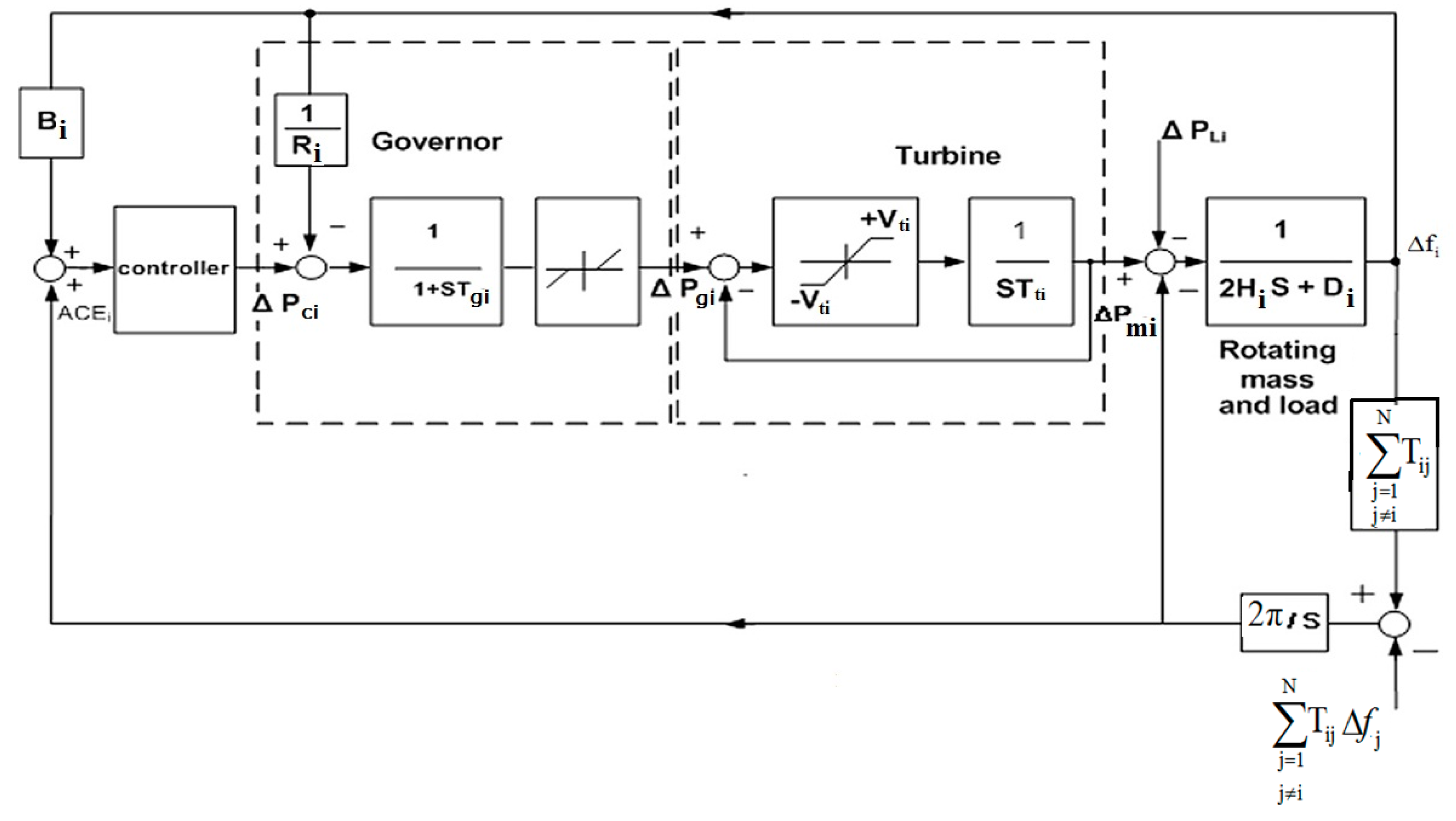
Figure 1 shows a power system with N control areas [1].

Figure 1. Dynamic model of a control area in an interconnected environment.

Figure 1. Dynamic model of a control area in an interconnected environment.

The model of frequency response for any area i of N power system control areas can be described as [2]:

$$\dot{∆f_i}=\left(\frac{1}{2H_i}\right)∆P_{mi}-\left(\frac{1}{2H_i}\right)∆P_{Li}-\left(\frac{D_i}{2H_i}\right)∆f_i-\left(\frac{1}{2H_i}\right)∆P_{tie,i}$$

(1)

While the dynamic of the governor can be expressed as:

$$\dot{∆P_{mi}}=\left(\frac{1}{T_{ti}}\right)∆P_{gi}-\left(\frac{1}{T_{ti}}\right)∆P_{mi}$$

(2)

And the dynamic of the turbine can be expressed as:

$$\dot{∆P_{gi}}=\left(\frac{1}{T_{gi}}\right)∆P_{ci}-\left(\frac{1}{R_i{T}_{gi}}\right)∆f_i-\left(\frac{1}{T_{gi}}\right)∆P_{gi}$$

(3)

The total tie-line power change between area i and the other areas can be calculated as:

$${\dot{∆P}}_{tie,i}=2\pi .\left[{\displaystyle \sum }_{\begin{array}{c}j=1\\ j\ne i\end{array}}^N{T}_{ij}∆f_i-{\displaystyle \sum }_{\begin{array}{c}j=1\\ j\ne i\end{array}}^N{T}_{ij}∆f_j\right]$$

(4)

Where$(∆)$ is a differential operator.

Also, the frequency deviation is added to the tie-line flow deviation in the supplementary feedback control loop to maintain the net interchange power with neighboring areas according to scheduled values. The area control error (ACE) represents the linear combination of tie-line power changes and frequency for area i, and is known as,

$$AC{E}_i=B_i∆f_i+P_{tie,i}$$

(5)

Equations (1)–(4) represent the frequency response model for $N$power system control areas with one generator unit in each area, and can be combined in the following state space model:

$$\left\{\begin{array}{l}\left[\begin{array}{c}\stackrel{•}{\Delta P_{gi}}\\ \stackrel{•}{\Delta p_{mi}}\\ \stackrel{•}{\Delta f_i}\\ \stackrel{•}{\Delta p_{tie,i}}\end{array}\right]=\left[\begin{array}{cccc}-\frac{1}{T_{gi}}& 0& -\frac{1}{R_i{T}_{gi}}& 0\\ \frac{1}{T_{ti}}& -\frac{1}{T_t}& 0& 0\\ 0& \frac{1}{2H_i}& -\frac{D}{2H_i}& -\frac{1}{2H_i}\\ 0& 0& 2\pi .{\displaystyle \sum _{\begin{array}{l}i=1\\ j=1\end{array}}^N{T}_{ij}}& 0\end{array}\right]\cdot \left[\begin{array}{c}\Delta P_{gi}\\ \Delta p_{mi}\\ \Delta f_i\\ \Delta p_{tie,i}\end{array}\right]+\left[\begin{array}{cc}0& 0\\ 0& 0\\ -\frac{1}{2H_i}& 0\\ 0& -2\pi \end{array}\right]\cdot \left[\begin{array}{c}\Delta p_{Li}\\ \Delta {\nu }_i\end{array}\right]+\left[\begin{array}{c}\frac{1}{T_{gi}}\\ 0\\ 0\\ 0\end{array}\right]\cdot \Delta p_{Ci}\\ y_i=AC{E}_i=\left[\begin{array}{cccc}0& 0& B_i& 1\end{array}\right].\left[\begin{array}{c}\Delta P_{gi}\\ \Delta p_{mi}\\ \Delta f_i\\ \Delta p_{tie,i}\end{array}\right]\end{array}\right\}$$

(6)

Where:

$∆f_i$: the frequency deviation of area i.

$∆P_{gi}$: the governor output change of area i.

$∆P_{mi}$: the mechanical power change of area i.

$∆P_{tie,i}$: the total tie-line power change between area i and the other areas.

$∆P_{Li}$: the load change of area i.

$∆P_{ci}$: supplementary control action of area i.

$y_i$: the system output of area i.

$H_i$: equivalent inertia constant of area i.

$D_i$: equivalent damping coefficient of area i.

R_i: speed droop characteristic of area i.

$AC{E}_i$: the control error of area i.

$T_{gi}$,$T_{ti}$: governor and turbine time constants of area i.

B_i: a frequency bias factor of area i.

T_ij: tie-line synchronizing coefficient with area j.

$∆v_i$: control area interface,$v_i=\left[{\displaystyle \sum }_{\begin{array}{c}j=1\\ j\ne i\end{array}}^N{T}_{ij}∆f_j\right]$.

3. Coefficient Diagram Method

The coefficient diagram method (CDM) is an algebraic design method which uses a coefficient diagram instead of a Bode diagram, and its theoretical basis is constituted using the condition for stability by Lipatov [10].

The coefficient diagram gives significant information about the system’s time response, stability, and robustness characteristics in one diagram, where the horizontal axis shows the order i values corresponding to each coefficient, whereas the logarithmic vertical axis shows stability indices (γ_i), the equivalent time constant (τ), and the characteristic polynomial coefficients (a_i). The measure of stability can be obtained using the degree of convexity derived from coefficients of the characteristic polynomial, while the speed of response can be calculated by the general slope of the curve. The shape of the a_i curve indicates the measure of robustness [11,12,13].

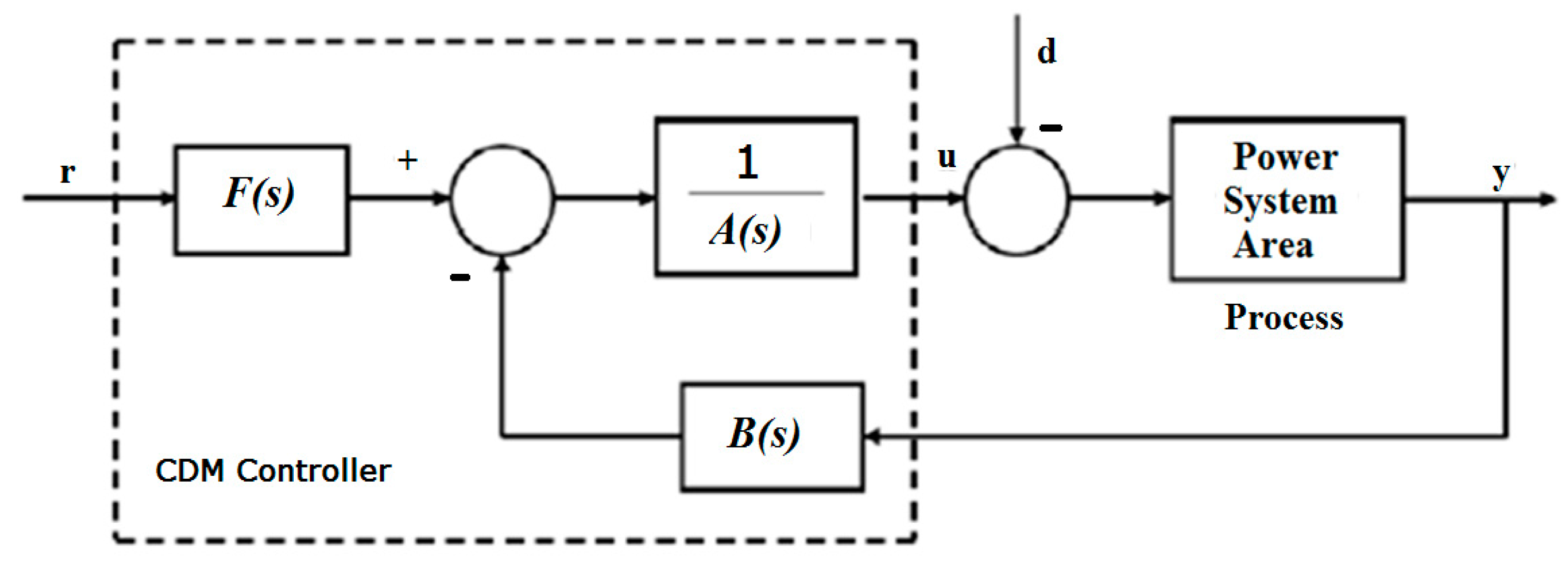
Figure 2 shows the block diagram of a single-input single-output (SISO) linear time invariant system with CDM control.

Figure 2. A block diagram of a CDM control system.

Figure 2. A block diagram of a CDM control system.

where:

D(s) is the denominator polynomial of the plant transfer function;

N(s) is the numerator polynomial;

A(s) is considered as the forward denominator polynomial;

F(s) and B(s) are considered as the reference numerator and feedback numerator polynomials.

In this method, d is the external disturbance signal, r is taken as the reference input to the system, u as the controller signal, and y is the output of the control system.

$$y=\frac{N\left(s\right)F\left(s\right)}{P\left(s\right)}r+\frac{A\left(s\right)N\left(s\right)}{P\left(s\right)}d$$

(7)

Where P(s) represents the characteristic polynomial of the closed-loop system and is defined by

$$P\left(s\right)=A\left(s\right)D\left(s\right)+B\left(s\right)N\left(s\right)$$

(8)

A(s) and B(s) are considered as the control polynomials and are defined as

$$A\left(s\right)={\displaystyle \sum }_{i=0}^P{l}_i{s}^{i}andB\left(s\right)={\displaystyle \sum }_{i=0}^q{k}_i{s}^i$$

(9)

For practical realization, the condition p ≥ q must be satisfied. To get the characteristic polynomial P(s), the controller polynomials from Equation (3) are substituted in Equation (2) and are given as

$$P\left(s\right)={\displaystyle \sum }_{i=0}^P{l}_i{s}^{i}D\left(s\right)+{\displaystyle \sum }_{i=0}^q{k}_i{s}^{i}N\left(s\right)={\displaystyle \sum }_{i=0}^n{a}_i{s}^i,a_i>0$$

(10)

Some parameters are needed for the design of the CDM, such as the stability indices (γ_i), the equivalent time constant (τ), and the stability limits (γ_i^*). The relations between these parameters and the coefficients of the characteristic polynomial (a_i) can be described as follows:

$${\gamma }_i=\frac{a_i^2}{a_{i+i}{a}_{i-1}},i\in \left[1,n-1\right],{\gamma }_0={\gamma }_n=\infty$$

(11)

$$\tau =\frac{a_1}{a_0}$$

(12)

$${\gamma }_i^{*}=\frac{1}{{\gamma }_{i-1}}+\frac{1}{{\gamma }_{i+1}},i\in \left[1,n-1\right]$$

(13)

γ_i values are selected as {2.5, 2, 2 ...2} according to Manabe’s standard form. These values can be changed by the designer. The target characteristic polynomial, $P_{target}\left(s\right)$, can be framed using the key parameters (τ and γ_i), as in

$$P_{target}=a_{°}\left[\left\{{\displaystyle \sum }_{i=2}^n\left({\displaystyle \prod }_{j=1}^{i-1}\frac{1}{{\gamma }_{i-j}^j}\right){\left(\tau s\right)}^i\right\}+\tau s+1\right]$$

(14)

where $P\left(s\right)=P_{target}\left(s\right)$.

In addition, the reference numerator polynomials F(s) can be calculated from:

$$F\left(s\right)=\frac{\left(P\left(s\right){|}_{s=0}\right)}{N\left(s\right)}$$

(15)

The coefficient diagram can be provided as the following example, when the plant and controller polynomials are given as [14].

$$\begin{gathered} N\left(s\right)=0.25s^4+s^3+2s^2+0.5s,D\left(s\right)=1 \\ A\left(s\right)=l_{1}s,B\left(s\right)=k_2{s}^2+k_{1}s+k_0 \\ {l}_1=1,k_2=1.5,k_1=1,k_0=0.2 \end{gathered}$$

(16)

The characteristic polynomial is expressed as

$$P\left(s\right)=0.25s^5+s^4+s^3+2s^2+s+0.2$$

(17)

Then

$$a_i=\left[a_5\dots a_2{a}_1\right]=\left[0.2512210.2\right]$$

(18)

$${\gamma }_i=\left[{\gamma }_4\dots {\gamma }_2{\gamma }_1\right]=\left[2222.5\right]$$

(19)

$$\tau =5$$

(20)

$${\mathsf{\gamma }}_i^{*}=\left[{\mathsf{\gamma }}_4^{*}\dots {\mathsf{\gamma }}_2^{*}{\mathsf{\gamma }}_1^{*}\right]=\left[0.510.90.5\right]$$

(21)

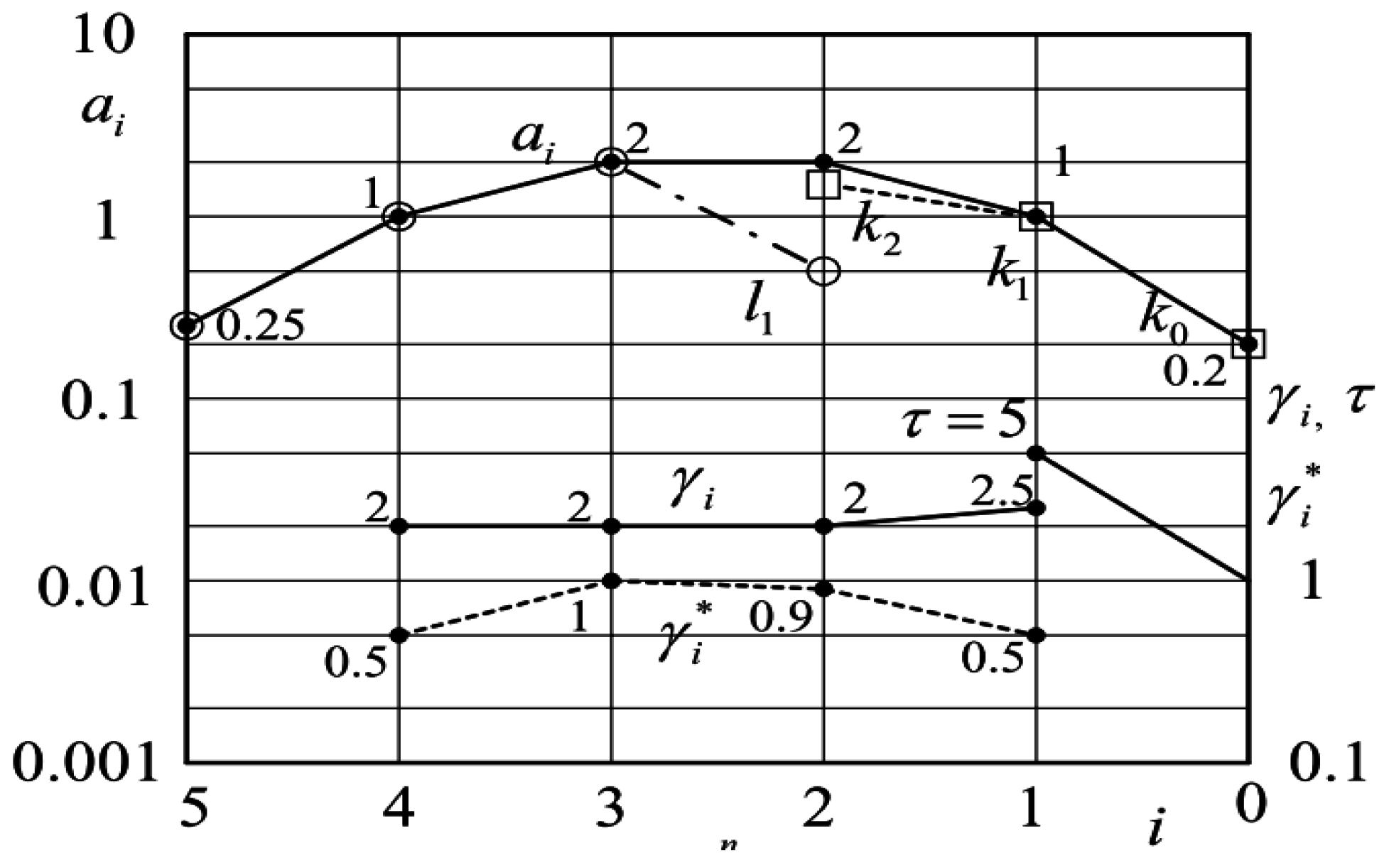
The coefficient diagram is shown as in Figure 3, where the coefficient of the characteristic polynomial (a_i) is read by the left-side scale, and the stability index (γ_i), stability limits (γ_i^*), and equivalent time constant (τ) are read by the right-side scale. The degree of convexity, which is obtained from coefficients of the characteristic polynomial, gives a measure for stability, while the general inclination of the curve gives a measure for the speed of response. If the curvature of a_i becomes larger, the system becomes more stable, corresponding to a larger γ_i. If the a_i curve is right down the τ, this means that the speed of the system response is fast. The variation of the shape of the a_i curve due to plant parameter variation is a measure of robustness.

Figure 3. Coefficient diagram.

Figure 3. Coefficient diagram.

4. LQG

The name LQG arises from the use of an integral cost function, a linear model, and Gaussian white noise processes to noise signals and model disturbances. The Kalman filter and optimal state feedback gain "k" are the two main parts of the LQG controller. The optimal feedback gain is calculated such that the feedback control law u = −kx minimizes the performance index:

$$H=\underset{0}{\overset{\infty }{{\displaystyle \int }}}\left(X^{T}QX+u^{T}Ru\right)dt$$

Where R and Q are positive definite or semi-definite real symmetric or Hermittian matrices [15]. The optimal state feedback u = −kx needs full state measurement. In our case, the states are chosen to be the frequency deviation$∆f$, mechanical power change$∆{\text{P}}_{\text{mi}}$, the governor output change $∆P_{gi}$, and the area tie-line power change $∆P_{tie,i}$. The frequency deviation $∆f_i$, the area tie-line power change $∆P_{tie,i}$and the supplementary control action $∆P_{ci}$ are chosen to be the measured signals which are fed to the Kalman estimator. The Kalman filter estimator is used to drive the state estimation:

$$\begin{array}{c}{\widehat{x}}_i\end{array}=\left[\begin{array}{ccc}∆{\widehat{f}}_i∆{\widehat{p}}_{mi}& ∆{\widehat{p}}_{gi}& ∆{\widehat{p}}_{tie,i}\end{array}\right]$$

Such that u = −kx remains optimal for the output feedback problem. The state estimation is generated from

$$\left(\widehat{\dot{x}}\right)=\left(A-Bk-LC\right)\widehat{x}+Ly$$

Where L is the Kalman gain and can be calculated by knowing the measurement covariance and system noise R_n and Q_n. The Kalman filter’s parameters and the LQG gains have been calculated off-line.

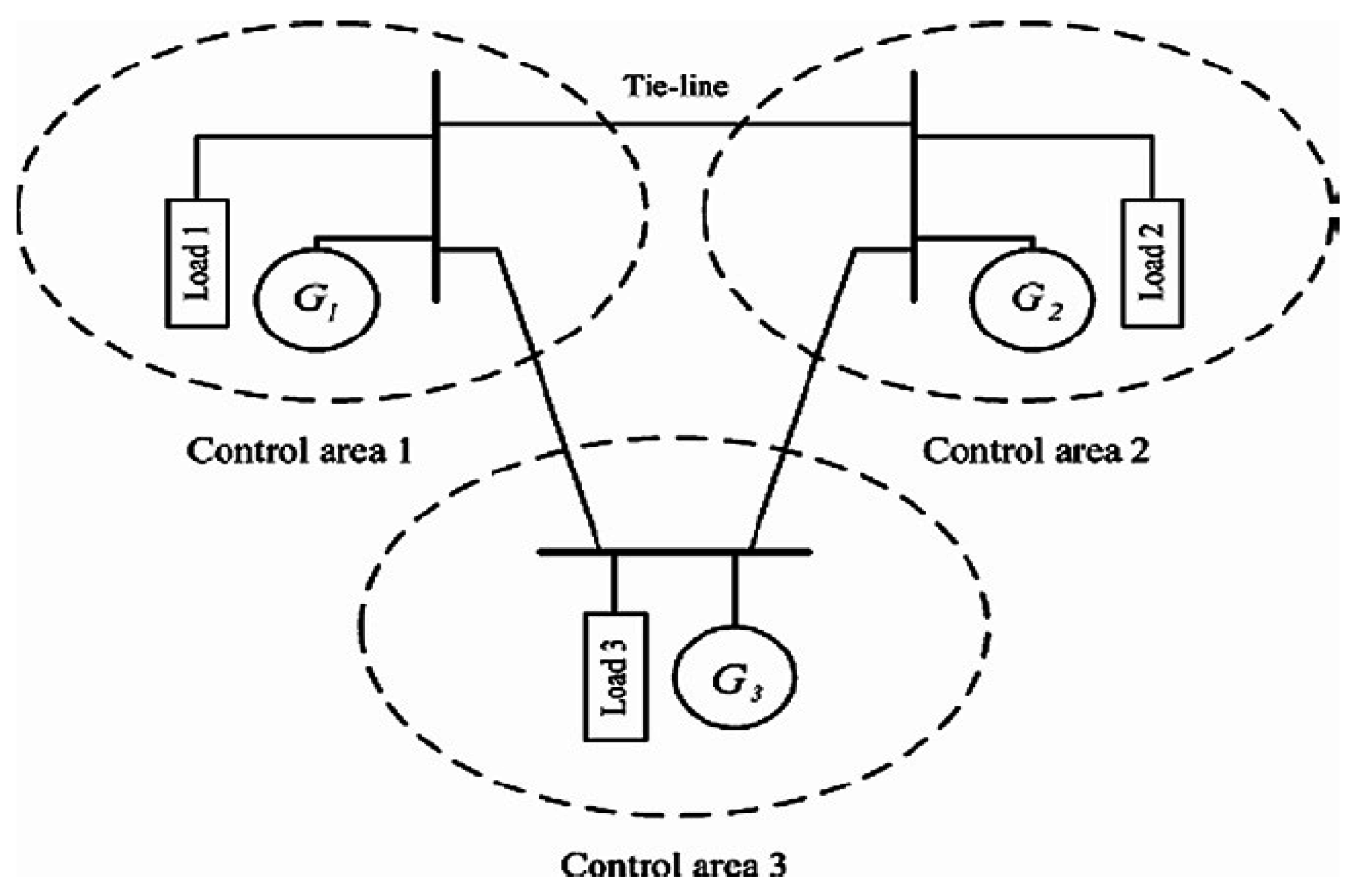
5. Case Study

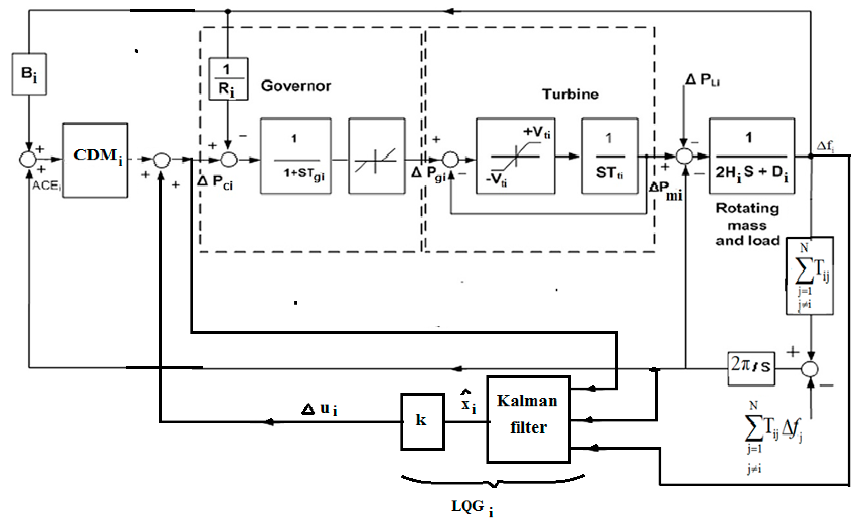
The three-area power system shown in Figure 4 is used to check the system performance with the proposed control method. As shown in Figure 5, each area has its own controller. The frequency deviation is used as a feedback for the closed-loop control system. The main control action can be calculated by adding the area control error ACE_i to the CDM controller. In addition, the supplementary control action $∆P_{ci}$, frequency deviation $∆f_i$, and the tie-line power change have been applied to the input of the Kalman filter to estimate the system states $\begin{array}{c}{\widehat{\text{x}}}_{\text{i}}\end{array}=\left[\begin{array}{ccc}∆{\widehat{f}}_i∆{\widehat{p}}_{mi}& ∆{\widehat{p}}_{gi}& ∆{\widehat{p}}_{tie,i}\end{array}\right]$, and these estimated states have been multiplied by optimal state feedback gain "k" to give the optimal control signal which, added to the main control signal to give supplementary control action$∆P_{ci}$, add to the negative frequency feedback signal. In addition, the area control error ACE_i can be calculated by summing the tie-line flow deviation to the frequency deviation.

Figure 4. Three-control-area power system.

Figure 4. Three-control-area power system.

Figure 5. The block diagram of multi-area power system including the proposed CDM + LQG controllers.

Figure 5. The block diagram of multi-area power system including the proposed CDM + LQG controllers.

6. Results and Discussions

The Matlab/Simulink software package has been used to check the effectiveness of the proposed scheme, and the system under study is three identical interconnected control areas, as shown in Figure 4, where the simulation parameters [2] are given in Table 1.

Table 1. Parameters and data of a practical three-control-area power system ((P_e)_Base = 800 MVA).

Area	K (s)	D (pu/Hz)	2H (pu/s)	R (Hz/pu)	Tg (s)	Tt (s)	Tij
Area-1	−0.3/s	0.015	0.1667	3.00	0.08	0.40	T12 = 0.20
							T13 = 0.25
Area-2	−0.2/s	0.016	0.2017	2.73	0.06	0.44	T21 = 0.20
							T23 = 0.15
Area-3	−0.4/s	0.015	0.1247	2.82	0.07	0.3	T31 = 0.25
							T32 = 0.15

Table 1. Parameters and data of a practical three-control-area power system ((P_e)_Base = 800 MVA).

Area	K (s)	D (pu/Hz)	2H (pu/s)	R (Hz/pu)	Tg (s)	Tt (s)	Tij
Area-1	−0.3/s	0.015	0.1667	3.00	0.08	0.40	T12 = 0.20
							T13 = 0.25
Area-2	−0.2/s	0.016	0.2017	2.73	0.06	0.44	T21 = 0.20
							T23 = 0.15
Area-3	−0.4/s	0.015	0.1247	2.82	0.07	0.3	T31 = 0.25
							T32 = 0.15

The parameters of the CDM controller of each area are detailed in [10], $andforLQG:$

K₁ = [−0.0638 0.2795 0.0482 −0.3229]

K₂ = [−0.0997 0.6735 0.1128 −0.7211]

K₃ = [0.0120 0.6133 0.0978 −0.6458]

The maximum value of the dead band for the governor is specified as 0.05 pu, and the generation rate constraint (GRC) of 10% per minute is applied for each area considered in the simulation [2].

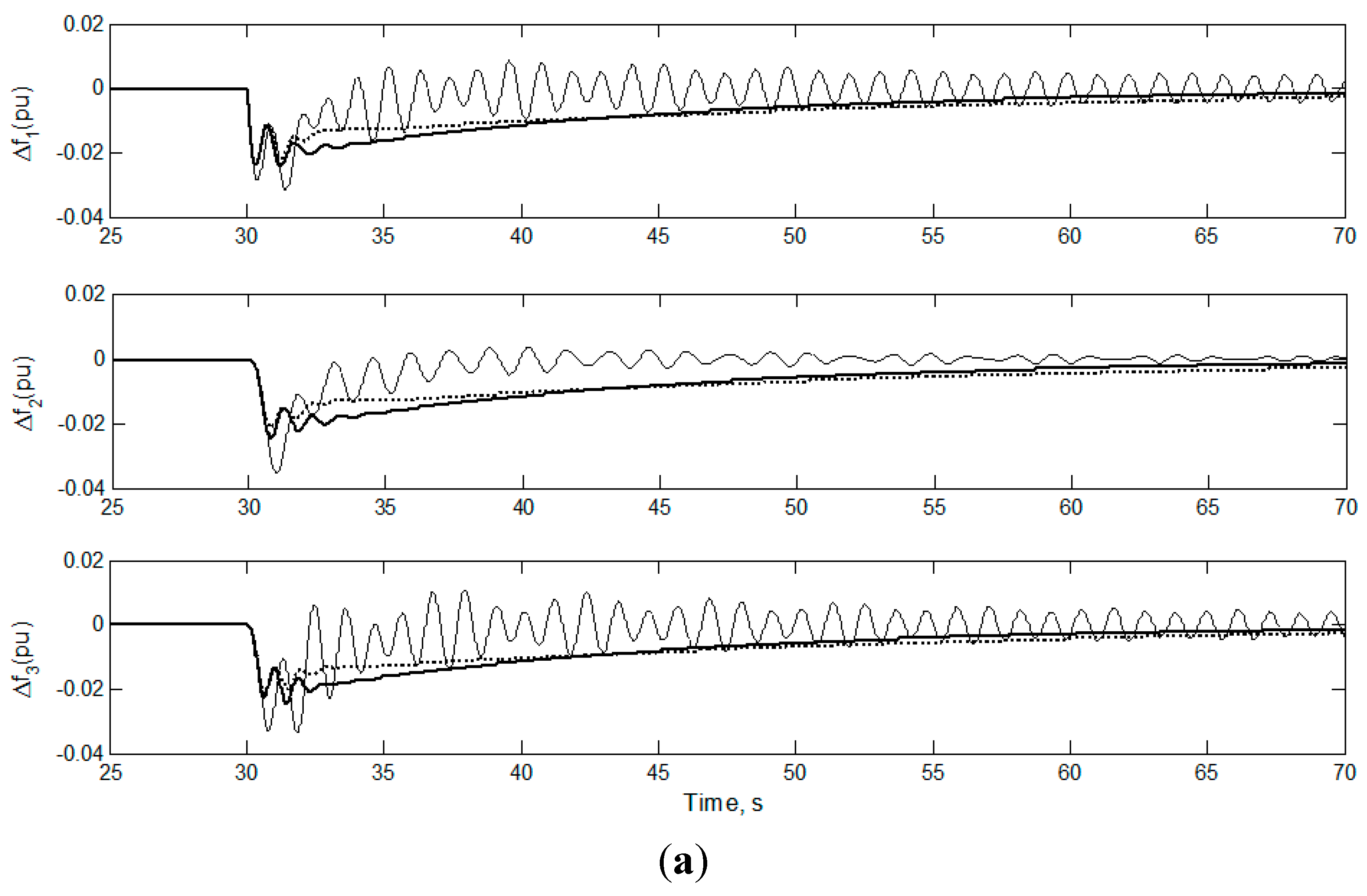
6.1. Case 1

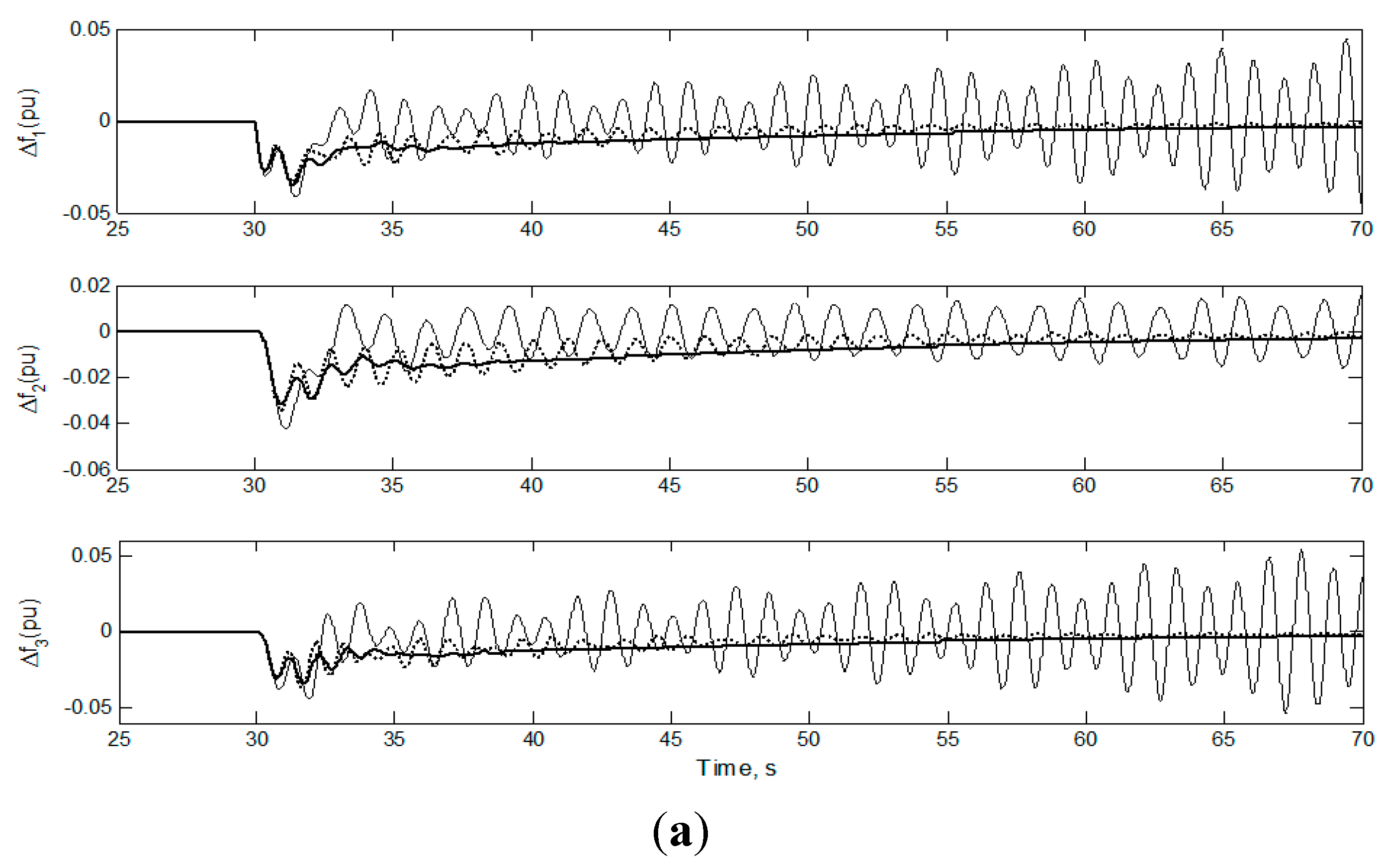
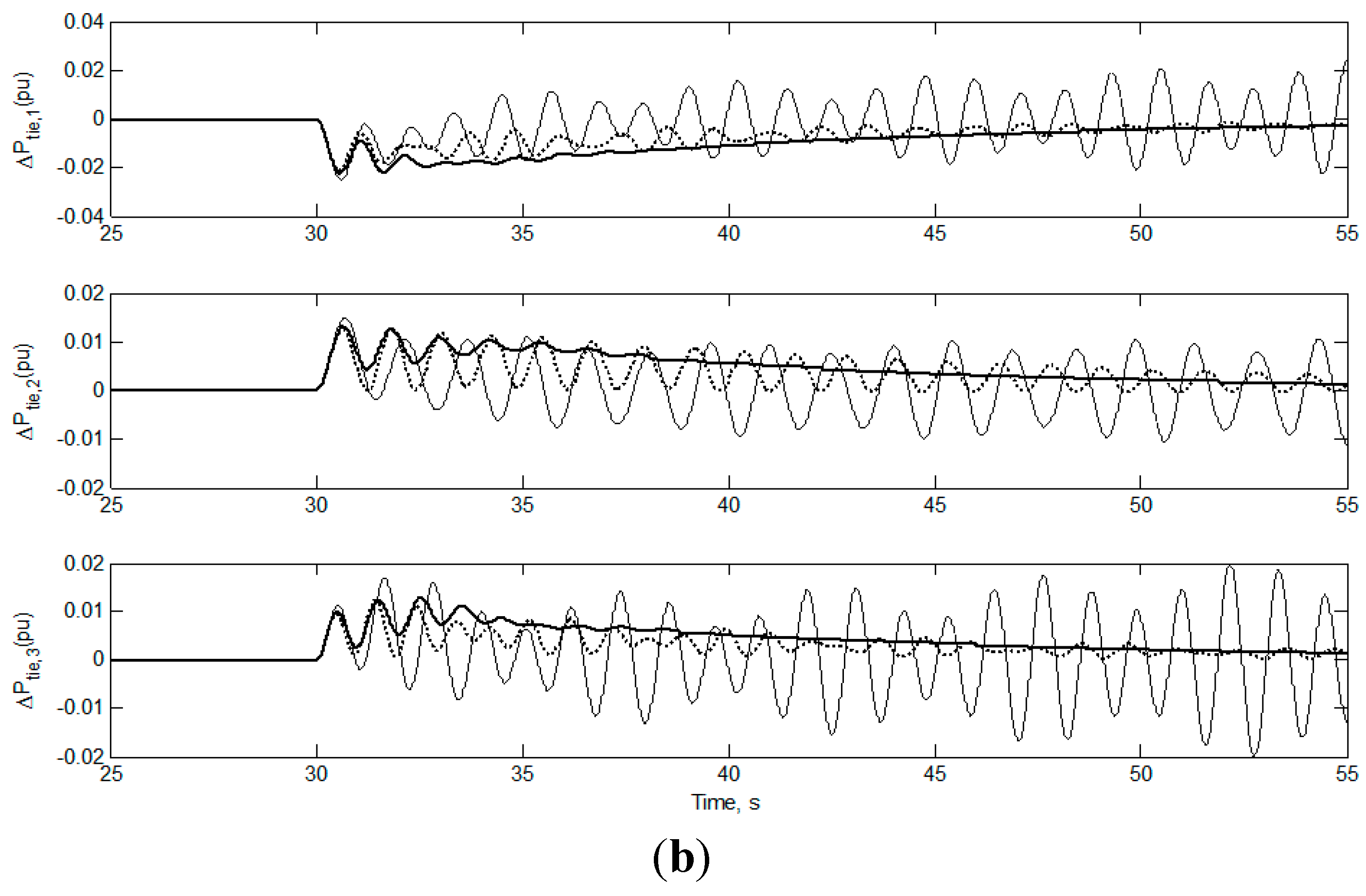
The system performances with the proposed CDM + LQG controller, only CDM, and the conventional integral controller are tested at nominal parameters and load change in area-1 ($∆{\text{P}}_{\text{L}1}$ assumed to be 0.02 pu at t = 30 s). Figure 6 shows the simulation results in this case. Figure 6a illustrates the frequency deviation for each area, and Figure 6b shows the tie-line power change for each area. It is obtained that the systems with both CDM + LQG and only CDM controllers are more stable and fast when compared to the system with a traditional integrator.

Figure 6. System response to the first case: (a) frequency deviations; (b) tie-line powers. CDM + LQG (solid line), CDM (dashed line), and conventional integrator (solid and thin line).

Figure 6. System response to the first case: (a) frequency deviations; (b) tie-line powers. CDM + LQG (solid line), CDM (dashed line), and conventional integrator (solid and thin line).

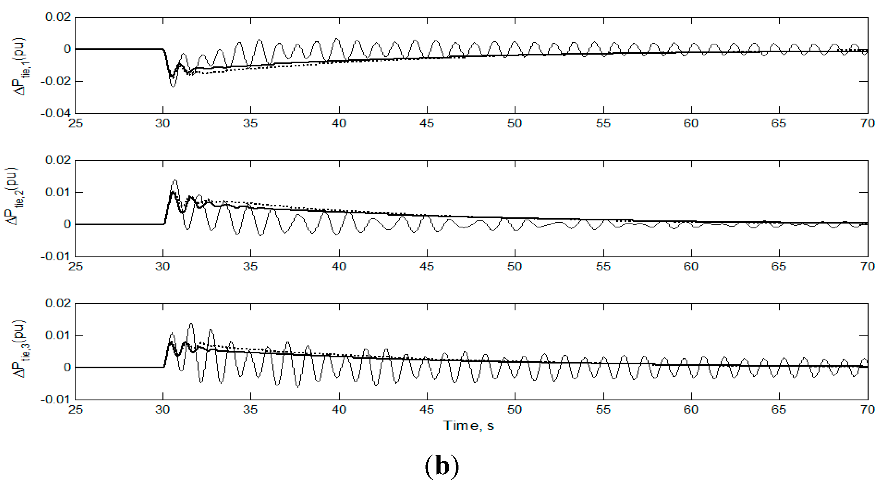
6.2. Case 2

The robustness of the proposed CDM + LQG controller in the face of a wide range of parameter uncertainties is validated, where the turbine and governor time constants of each area are increased to T_t1 = 0.785 s (≅95% change), and T_g1 = 0.105 s (≅31% change), T_t2 = 0.6 s (≅38% change), and T_g2 = 0.105 s (≅66% change), T_t3 = 0.7 s (≅100% change), and T_g3 = 0.15 s (≅100% change), respectively.

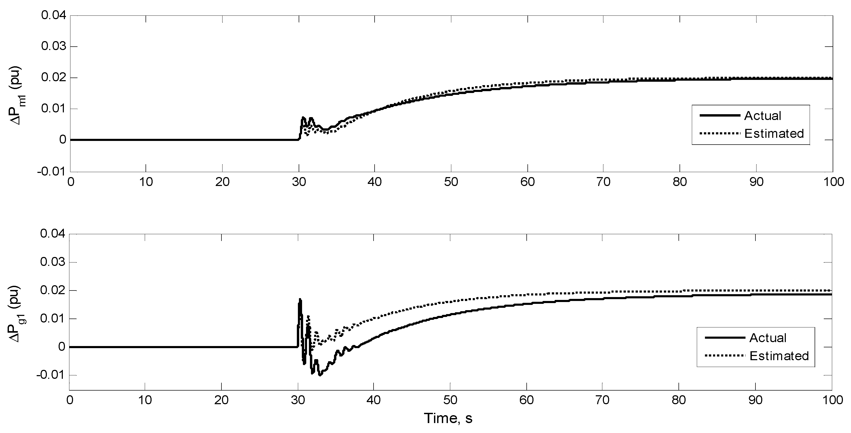
Figure 7 depicts the responses of the three controllers in the presence of the above uncertainty, at load change in area-1 ($∆{\text{P}}_{\text{L}1}$ assumed to be 0.02 pu at t = 30 s). It has been indicated that compared with only the CDM controller, a desirable performance response has been achieved using the proposed CDM + LQG, while with the conventional integrator the case was unstable. In addition, Figure 8 illustrates the actual and estimate$∆{\text{P}}_{\text{gi}}$ and $∆{\text{P}}_{\text{mi}}$ for each area, as shown in the figure, and the good effort of the Kalman filter led to a positive impact on the performance of LQG.

Figure 7. System response to the second case: (a) frequency deviations; (b) tie-line powers. CDM + LQG (solid line), CDM (dashed line), and conventional integrator (solid and thin line).

Figure 7. System response to the second case: (a) frequency deviations; (b) tie-line powers. CDM + LQG (solid line), CDM (dashed line), and conventional integrator (solid and thin line).

Figure 8. Estimated and actual $∆P_{m1},∆P_{g1}$

Figure 8. Estimated and actual $∆P_{m1},∆P_{g1}$

7. Conclusions

A robust distributed LFC design using both CDM and LQG has been proposed for an interconnected power system and has been presented in this paper. A three-area power system is used to check the effectiveness of all of the proposed control strategies, the conventional integrator and CDM alone, under load change and parameter change cases.

From the results, it was shown that the power system with both CDM + LQG and CDM controllers is robust in face of load change and parameter perturbation, and the system has a more desirable performance as compared to the classical integral controller design. Also, it is indicated that the proposed CDM + LQG can give a desirable and smooth response.