A Local Texture-Based Superpixel Feature Coding for Saliency Detection Combined with Global Saliency

Abstract

Because saliency can be used as the prior knowledge of image content, saliency detection has been an active research area in image segmentation, object detection, image semantic understanding and other relevant image-based applications. In the case of saliency detection from cluster scenes, the salient object/region detected needs to not only be distinguished clearly from the background, but, preferably, to also be informative in terms of complete contour and local texture details to facilitate the successive processing. In this paper, a Local Texture-based Region Sparse Histogram (LTRSH) model is proposed for saliency detection from cluster scenes. This model uses a combination of local texture patterns and color distribution as well as contour information to encode the superpixels to characterize the local feature of image for region contrast computing. Combining the region contrast as computed with the global saliency probability, a full-resolution salient map, in which the salient object/region detected adheres more closely to its inherent feature, is obtained on the bases of the corresponding high-level saliency spatial distribution as well as on the pixel-level saliency enhancement. Quantitative comparisons with five state-of-the-art saliency detection methods on benchmark datasets are carried out, and the comparative results show that the method we propose improves the detection performance in terms of corresponding measurements.

1. Introduction

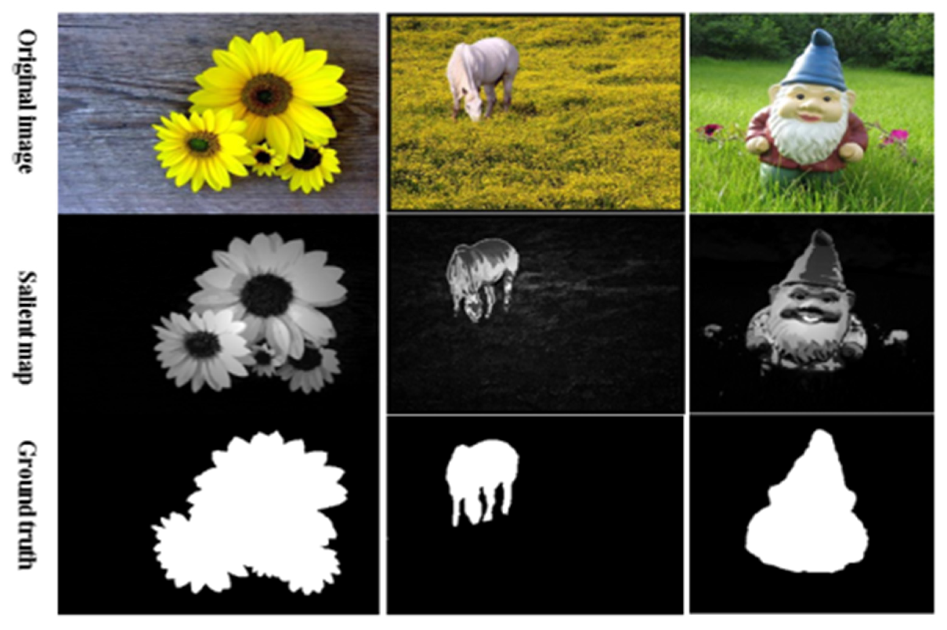
Saliency detection has continuously been one of the focuses of research in the computer vision field. As indicated in recent applications in image segmentation [1], object detection [2], image retrieval based on content [3], image classification [4], image semantic understanding [5], etc., progress on saliency detection research is one of the principal factors leading to performance improvement of work in the relevant field. In general, saliency detection should meet the following criteria: (1) The salient object/region detected needs to be accurately located in images, which is ideally coherent with humans perceiving focus of region/object in cluster scenes. (2) The salient object/region detected needs to be clearly distinguished from complex background, while, ideally, retaining the information integrity of the object/region, such as inherent complete contour and local texture details as much as possible to facilitate successive image processing and analysis. (3) Saliency detection should be performed within an acceptable timescale, and the overhead of the computation involved should be low [6] (Figure 1).

Figure 1. An example comparison of original images, salient maps and ground truth; from top to bottom: original images, salient maps and ground truth.

Figure 1. An example comparison of original images, salient maps and ground truth; from top to bottom: original images, salient maps and ground truth.

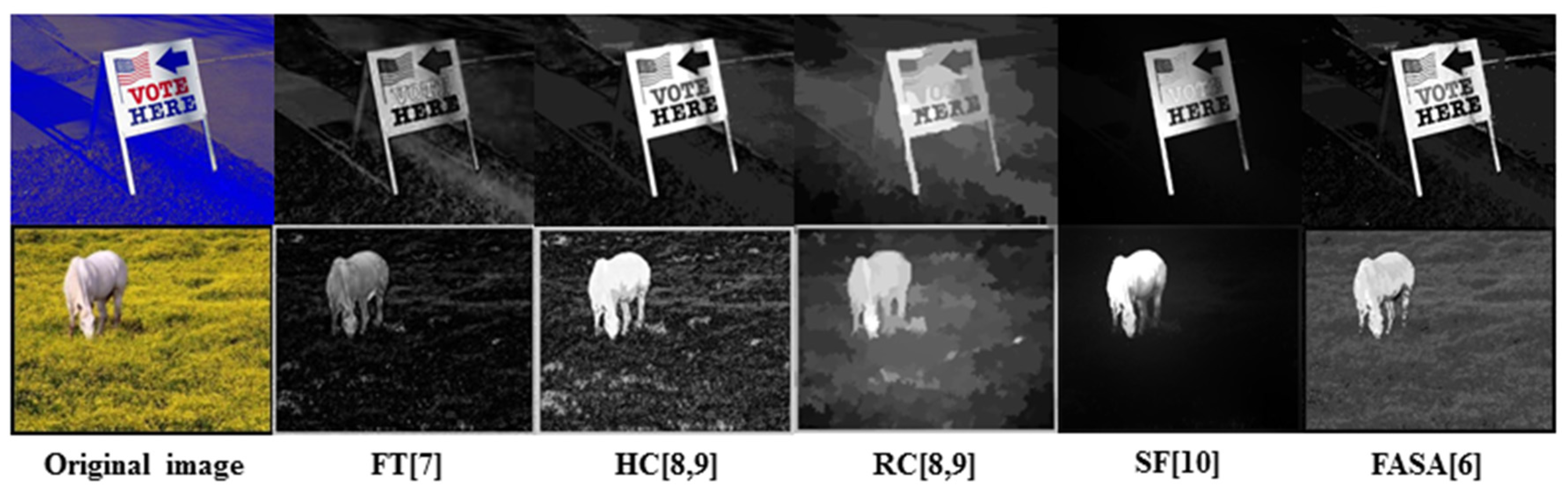
In accordance with the human vision attention mechanism, visual saliency of an image is defined as how much a certain region/object in an image visually stands out from its surrounding area with high contrast. To detect the visual saliency as defined, there are many contrast-based methods recently reported in the literature, such as Frequency-Turned (FT) [7], Histogram-based Contrast (HC) [8,9], Region-based Contrast (RC) [8,9], SF (Saliency Filters) [10], and FASA (Fast, Accurate, and Size-Aware) [6]. However, FT [7] method directly defines each pixel’s color difference from the average color value of the whole image as the pixel’s contrast, therefore, the saliency detected in this method is sensitive to image edges and noise, and the performance of the detection is poor. Cheng et al. proposed HC and RC in [8,9]. Because both of the methods only use the color feature, saliency detection performed in these two methods often achieves a blurry salient map when working with cluttered images. Furthermore, SF [10] method, which is also based on contrast, combines global contrast and spatial relations together to generate the final salient map. However, in some cases, SF [10] method cannot differentiate the salient region/object with sufficiently complete contours and detailed local texture from a complex background. Although it is superior to the others in terms of speed, FASA [6] sometimes falsely marks the background as the salient region because the detection is also carried out using solely the color feature for calculating the global color contrast and saliency probability. 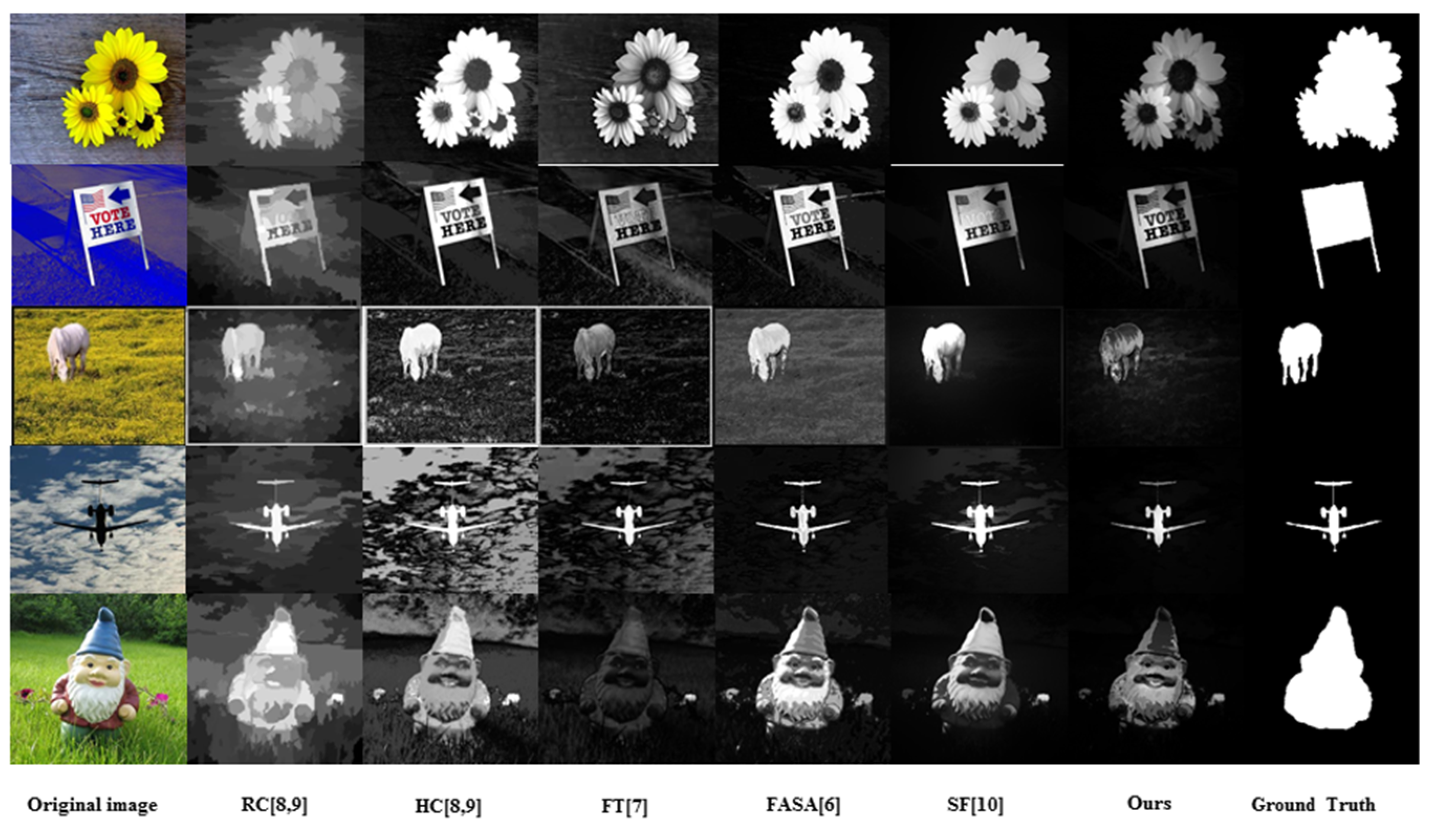Examples of saliency maps generated by FT [7], HC [8,9], RC [8,9], SF [10] and FASA [6] methods are shown in Figure 2, in which the defects of incomplete contour, blurred local texture details and the false marking of background as salient region can be visually identified in corresponding maps.

Figure 2. Examples of saliency maps generated by FT, HC, RC, SF and FASA methods.

Figure 2. Examples of saliency maps generated by FT, HC, RC, SF and FASA methods.

The figurative result in Figure 2 reveals by analysis that the reason the defects are induced lies in the fact that only information used in the detection process is the color feature, which is, apparently, insufficient. In contrast to the global color information, the local texture information, as one of the dominant visual features in the real world, presents important information about the smoothness, coarseness and regularity of an object’s local details. Therefore, it would be better to combine the local texture feature and the color feature together to enrich the information used in saliency detection, and hopefully improve the accuracy of salient region/object location and retaining the inherent information that the detected salient region/object possess.

There are many descriptors available for local region texture description. Among them, CS-LBP (Center Symmetric Local Binary Pattern) [11] and CS-LTP (Center Symmetric Local Trinary Pattern) [12] are popular representatives. In these two descriptors, the histogram that encodes the local texture feature of the region surrounding each pixel is constructed with the same number of bins, spreading over the full texton spectrum domain. It is not difficult to understand that, as the number of pixels involved increases, the computational load to compute the corresponding histograms also increases, which makes descriptors constructed in a similar way unsuitable for describing the region feature. Another problem with this histogram encoding is that it is not efficient. Because practically every local region contains a few types of textures, it is not necessary to generate the histogram over the whole range of the texton spectrum to avoid bringing in additional calculations. In addition, the histogram as constructed is a measure of the degree of similarity, not an indication of the differences of contrast among the local regions, and therefore it cannot be used for calculating the region contrast on which the saliency detection we propose is based.

Superpixel segmentation is now a commonly used image segmentation method. To some extent, a superpixel can be regarded as a region. Compared to the local region, as discussed above and normally selected as a circle surrounding each pixel with certain radius, a superpixel often has an irregular shape that contains the inherent feature of an object. Meanwhile, regarding a superpixel as a region, decreases the number of regions, implying a certain reduction in calculations compared to the pixel-based regionization methods.

Based on the analyses and discussions that have been conducted, a Local Texture-based Region Sparse Histogram model (LTRSH) is proposed in this paper. The model is superpixel based, and a combination of two histograms, one for local texture information and contour information and the other for color information, is used to describe the features of superpixels. The histograms are constructed on the base of sparse representation to enhance efficiency of the processing, and as created, they are also capable of measuring the differences of contrast among the local regions, which facilitates the computation of the region contrast.

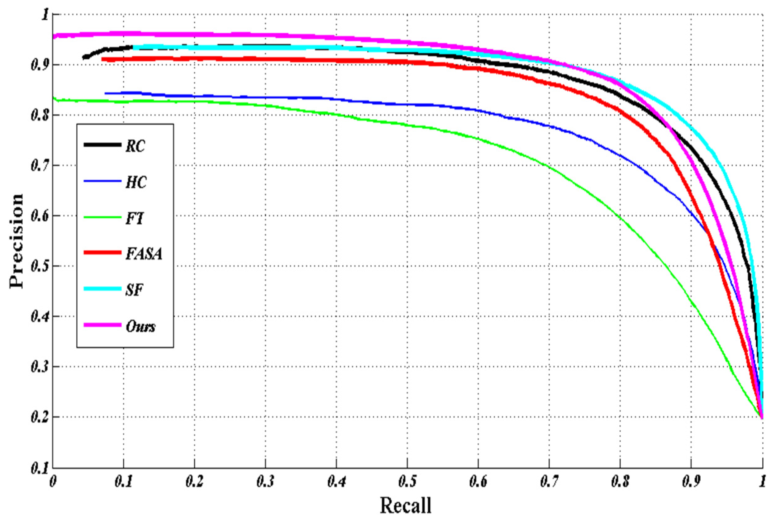
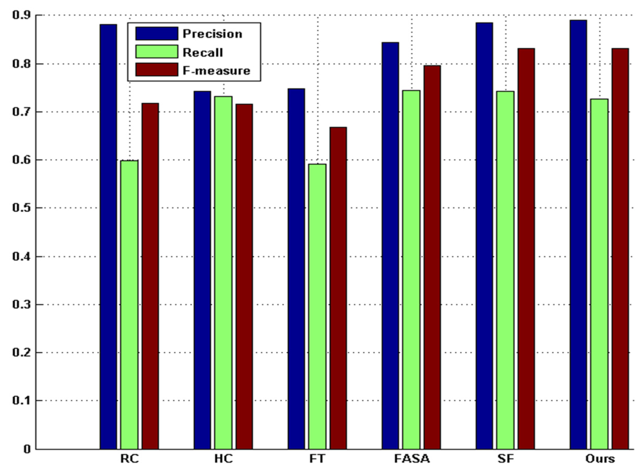
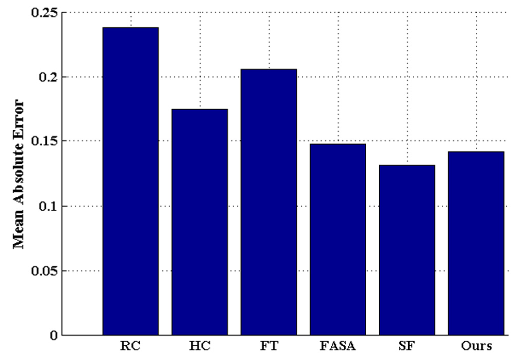
Extensive experimentation has been carried out to evaluate the method proposed in this paper against five state-of-the-art saliency detection methods [6,7,8,9,10] on benchmark datasets. The comparative results show that the proposed method is promising, as it improves the detection performance in terms of precision rate, recall rate, and F_β measurement.

2. Related Work

We can group existing methods for saliency detection into two categories according to their methodology: biologically motivated and purely computational.

After the method based on the biological model was first presented by Koch and Ullman [13], Itti et al. [14] proposed that image visual saliency was the central-surrounding difference when addressing multi-scale low-level features. However, their result was substantially less satisfactory. Harel et al. [15] obtained a salient map by normalizing Itti’s feature maps based on statistics (Graph-based (GB)), and their salient map was greatly improved over that of Itti’s. Geferman et al. [16] presented the Context-aware (CA) method to obtain the salient map with image contexts using local low-level clues, global considerations, visual organization rules and high-level features. However, the final saliency was usually not ideal, especially near the edges of the image, and suffered from slow computation. Recently, the RC [8,9] method was found to produce a better result by incorporating the color information and spatial information; however, it is neither full resolution nor efficient because it considers only the color feature at local scales, thus resulting in a fuzzy salient map with incomplete contours of the object/region and local texture information.

Computationally oriented methods can be divided into two groups based on feeding feature. The first group investigates the region’s visual saliency with respect to the feature of local neighborhoods. For instance, Ma et al. [17] (Ma and Zhang (MZ)) utilized the fuzzy growth model to generate the salient map; however, it was relatively time consuming and produced poor salient maps. Achanta et al. [18] generated average color difference in the multi-scale space from the average of their neighborhoods as the saliency (Average Contrast (AC)). Although a full-resolution salient map is presented, the precision and location are not accurate and appear to be sensitive to noise and complex texture. Liu et al. [19] obtained the saliency via multi-scale contrast and then linearly combined the contrast in a Gaussian image pyramid. In 2013, Li et al. [20] detected saliency by finding the vertices and hyperedges in a previously constructed hypergraph. In 2015, Lin et al. [21] addressed the problem of saliency detection by learning adaptive mid-level features to represent local image information and then calculated multi-scale and multi-level saliency maps to obtain the final saliency.

The other group uses global image feature in their computationally oriented method. Similar to Zhai and Shan’s L-channel Contrast (LC) [22] method, such methods only use the L-channel of an image to compute each pixel’s contrast. Hou et al. [23] proposed Spectral Residual (SR) to obtain the saliency in the frequency domain of an image. Although this method was computationally efficient in the frequency domain, it could not produce the full-resolution salient map and the result was unsatisfying. Achanta [7] presented FT method, which obtained a pixel’s saliency by measuring each pixel’s color difference from the average color in the image to exploit the spatial frequency content of the image. Finally, HC [8] method constructs the color histogram only using color to obtain the saliency; however, this method does not perform well with complex texture scenes in certain instances.

Recently, researchers have increasingly investigated methods of detecting image saliency by simultaneously considering the local and global feature, with some methods achieving better performance. For example, Perazzi et al. proposed a conceptually clear and intuitive algorithm (Saliency Filters (SF)) [10] for contrast-based saliency estimation based on the uniqueness and spatial distribution of those elements that combined the two measures in a single high-dimensional Gaussian filtering framework. In this way, they simultaneously addressed both local and global contrast; however, substantially more parameters are needed to produce satisfactory results because the method sometimes falsely identifies the background as the salient region. Yong et al. [24] proposed Cell Contrast and Statistics (CCS), which utilizes both the color contrast model and space statistical characteristic model to detect saliency based on the constructed image cell. In 2014, Gokhan et al. exploited the contributions of the visual properties of saliency in two methods. The first method [25] is based on machine learning and initially extracts biologically plausible visual features from the hierarchical image segments; then, it uses regression trees to learn the relationship between the feature value and visual information. The second method is FASA [6], which obtains a probability of saliency by feeding the statistical model with the spatial positions and sizes of the quantized colors estimated early and then combines the probability of saliency with the global color contrast measure to obtain the final saliency. Chen et al. [26] addressed multiple background maps in an attempt to generate full-resolution salient maps in linear computation time and with a low probability of falsely masking background as salient regions. However, the method would sometimes fail as a result of the background estimation being invalid.

Overall, recent improvements of saliency detection indicate that using the local feature combined with the global feature to accurately detect the salient object/region in the image is the general pursuit of mainstream research. The salient object/region would be clearly separated from cluster scenes with the overall shape or contour and subtle texture details. However, these existing methods have not effectively used the local texture information working together with color information for saliency detection.

3. Our Proposed Method

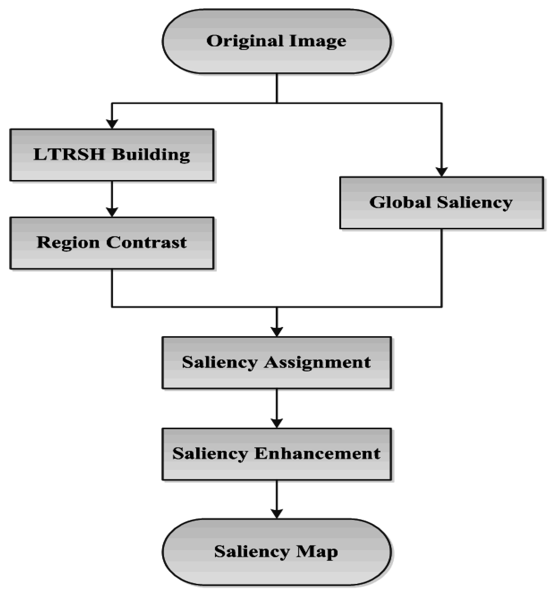
Therefore, our work is to first obtain the underlying color distribution with a near-uniform texture pattern in local detail to encode the superpixel for region contrast computing. Then, we combine the region contrast and the global saliency probability, obtained from the global color feature, together to detect the final salient object/region accurately located in the image with complete contour and local texture details. The scheme of our salient object/region detection method is illustrated in Figure 3.

Figure 3. The scheme of our method.

Figure 3. The scheme of our method.

We first build the LTRSH model that characterizes each superpixels’ inherent contour and local texture information as well as the color information to obtain the region’s contrast. Meanwhile, the probability of each pixel’s global saliency is determined based on the global color information. This process is similar to FASA [6] method, which can determine the rough shape of the salient object/region relative to the complete contour of the object/region if the object/region has a much more remarkable color feature. Then, we implement pixel-level saliency assignment using a combination of the region contrast and global saliency in pixel level. Finally, we enhance the saliency in pixel level according to the saliency distribution in global to ensure that the points that are farther from the center of the saliency have weaker saliency, and vice versa [10].

3.1. LTRSH Model Building

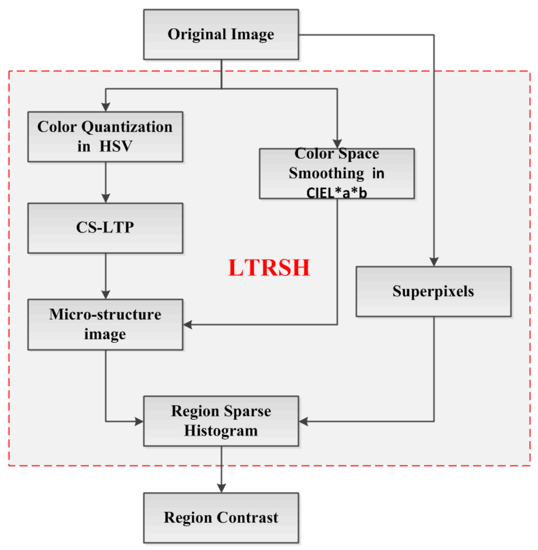
Our main contribution is building the LTRSH to encode the superpixel’s feature for obtaining the region contrast, which is displayed in the red rectangle in Figure 4.

Figure 4. The scheme of region contrast computation based on LTRSH.

Figure 4. The scheme of region contrast computation based on LTRSH.

In this proceeding, we firstly extract the CS-LTP [12] of the color quantization in HSV space, which captures the major texture and contour information. The reason for choosing the color in HSV space is that the HSV color space captures the local color texture features well in detail and can make effective use of color information. Moreover, the HSV color space is a uniform color space and non-linear transformation. It can better capture the components in the manner that humans perceive the color. Then, we detect the local texture pattern by encoding the CS-LTP [12] to produce the CS-LTP map. The CS-LTP can perform outstandingly at describing near-uniform image regions for extracting major texture and contour information. It can also smooth weak illumination gradients and filter out insignificant details such as the acuity of color and sharp changes in edge orientation. Meanwhile, with the color space smoothing in CIE L*a*b we use the CS-LTP map as a mask to produce a microstructure image that captures the region’s local texture information and the contour information. Finally, by describing the superpixels segmented from the original image, we construct the LTRSH model to encode each superpixel’s feature based on the microstructure image.

3.1.1. HSV Color Space and Color Quantization

Here, we adopt the HSV color space, and the quantization step is as follows. For a full-color image of size $h\times w$, we convert the image from RGB color space to HSV color space. Specifically, the H, S and V color channels are uniformly quantized into 12, 4 and 4 bins, respectively, thus the HSV color image is uniformly quantized into 192 levels.

In this way, we can describe the color feature of the image in one dimension based on Equation (1):

$$P=Q_s{Q}_{v}H+Q_{v}S+V$$

(1)

In Equation (1), $Q_s=4$ and $Q_s=4$ represent the number of quantizations for the color channels S and V, respectively. Therefore, the quantized color image is denoted as imageX (imageX = g, $g\in \left\{0,1,\mathrm{...},G-1\right\}$, G = 192).

3.1.2. Local Texture Pattern Detection

Local texture information is detected on the color quantization in HSV space by coding the local texture pattern to obtain one corresponding CS-LTP map T ($T(x,y)=x,x\in \left\{0,1,\mathrm{...},X-1\right\}$).

The CS-LTP map can be obtained through the following steps:

First, for each point $p_i(x_i,y_i)$ ($x_i$ and $y_i$ represent the coordinates of the point $p_i$) on imageX, starting from the right of point $p_i(x_i,y_i)$, we can locate $N$ ($N>0,N\in N^{+}$) points $\{p_i^k(x_i^k,y_i^k)\}$ $(k=1,2,\mathrm{...},N)$ orderly by tracing a circle with radius $R(R>0)$ in the clockwise direction, satisfying the constraint that is the distance between $p_i$ and the $kth$ point $p_i^k$ is equal to $x_i^k-x_i=R\cos \theta$, $y_i^k-y_i=-R\sin \theta$. Then, a pair of points $\{p_i^k,p_i^{k+N/2}\}$ can be obtained, and the quantized value of $\{p_i^k,p_i^{k+N/2}\}$ is denoted as $n_i^k$ and $n_i^{k+N/2}$ for $k=1,2,\mathrm{...},N/2$.

Next, the CS-LTP coding $T(x_i,y_i)$ of point $p_i(x_i,y_i)$ is defined as $(T(x_i,y_i)=x,x\in \left\{0,1,\mathrm{...},X-1\right\})$ (Equation (2)):

$$T_{R,N}(x_i,y_i)={\displaystyle \sum _{k=0}^{\frac{N}{2}-1}s(n_i^k-n_i^{k+\frac{N}{2}})3^k ，} s(j)=\{\begin{array}{c}2, j\ge t\\ 1, -t<j<t\\ 0, j\le -t\end{array}$$

(2)

where $t$ is the user-specified threshold. Here, we use the tolerance interval $t=0.8$. Thus, we know that when $R=1$ and $N=8$, CS-LTP is defined as having a length of 4 bits with the indicator $s(j)$, which is replaced with a three-valued function. In this way, $X$ of the CS-LTP map is ${\displaystyle \sum _{i=0}^{3}2\times 3^i}=81$. The reason for using CS-LTP is that CS-LTP is more resistant to noise, but is no longer strictly invariant to gray-level transformations [27].

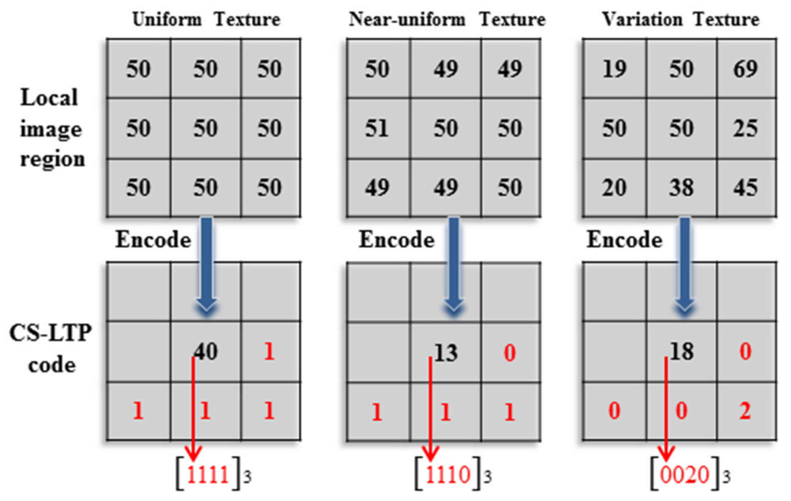
The procedure for local texture pattern coding is illustrated in Figure 5. For example, the third variation texture in Figure 5 is encoded as ${\left[0020\right]}_3$, and then, it is converted to the decimal number 18. In this case, the point $p_i(x_i,y_i)$ is encoded as 18 as the gray value of the CS-LTP map $T$.

Figure 5. An example of CS-LTP encoding (t = 0.8).

Figure 5. An example of CS-LTP encoding (t = 0.8).

3.1.3. Microstructure Image Production

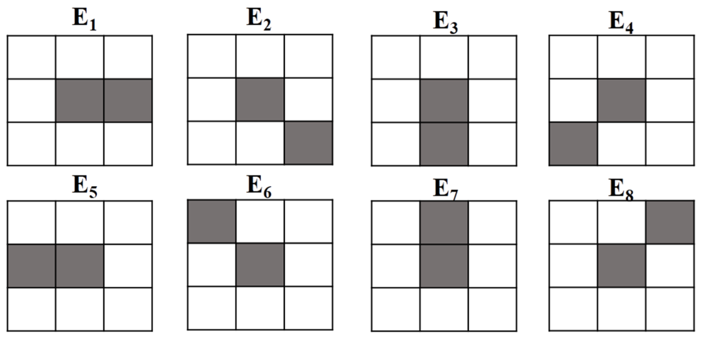
After local texture pattern detection, we use eight neighbors (shown in Figure 6), representing eight orientations, to produce a microstructure image using the CS-LTP map as a mask with the color space smoothing in CIE L*a*b. A microstructure image can characterize the local texture information and contour information by the color distribution with a near-uniform texture.

Figure 6. Eight structural elements used in the microstructure image.

Figure 6. Eight structural elements used in the microstructure image.

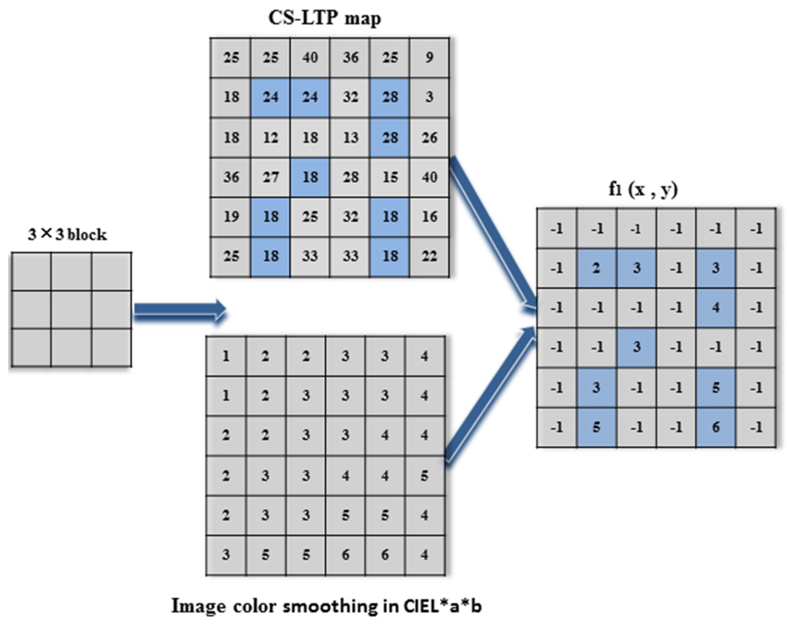
To remove insignificant details and better describe the near-uniform texture information, we start from the original point (0, 0), (1, 0), (0, 1) and (1, 1), and move in a $3\times 3$ block from left to right and top to bottom throughout the CS-LTP map $T$ to detect structural elements with the image color smoothing in CIE L*a*b to produce the microstructure image $f_i\text{,(}i\in \{1,2,3,4\})$. The procedure for $f_{\text{1}}$ can be observed in Figure 7.

Figure 7. Illustration of producing a microstructure image f₁.

Figure 7. Illustration of producing a microstructure image f₁.

According to Figure 7, when the starting block (0, 0) is centered at point 24 in the CS-LTP map $T$, only the right point among its eight neighbors is the same as point 24. Meanwhile, we locate the same location on the image color smoothing in CIE L*a*b. Then, we obtain 2 and 3 for the correspondent points and assign the other seven points with −1 for the correspondent points in microstructure image f₁, because the other seven correspondent points in the CS-LTP map $T$ are different from point 24. Then, we move the block to the next three point centers at point 28 to obtain the same point 3 and point 4 in microstructure image f₁. The remainder can be performed in the same manner, with the block moving from left to right and then down to produce the microstructure image f₁.

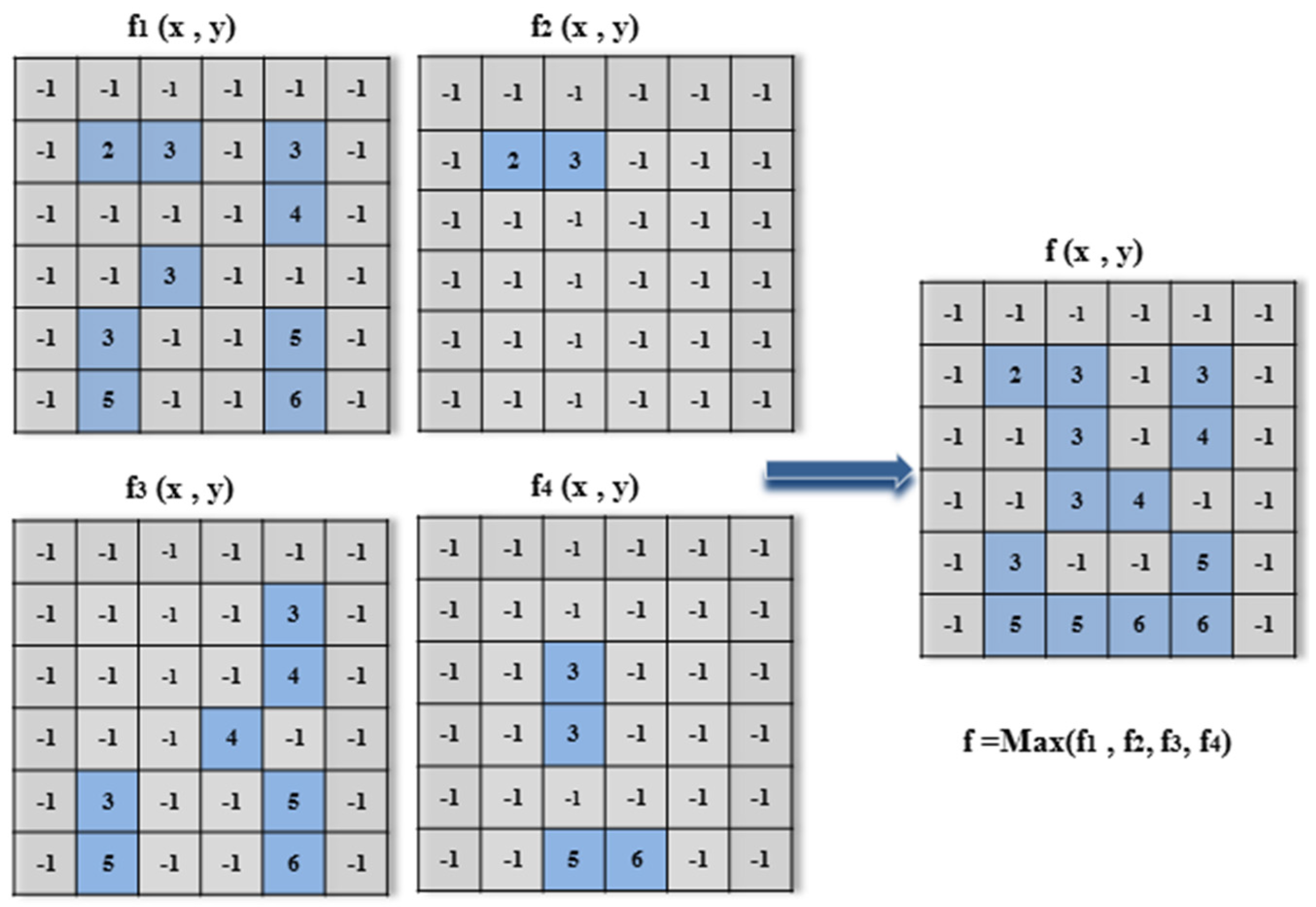
After we start from the original points (1, 0), (0, 1) and (1, 1) in the same way of gaining the microstructure image f₁, we obtain the microstructure images f₂, f₃, and f₄. Next, we determine the overall maximum of the images $f_i\text{ (}i\in \{1,2,3,4\})$ to obtain the final microstructure image f, as illustrated in Figure 8. In the final microstructure image $f(f(x,y)\in \{-1,0,1,\mathrm{...},G-1\})$, the point values $f(x,y)$ represent the category of color following the original image color smoothing, which are combined together to characterize the local region texture in detail and contour information, except for the value −1.

Figure 8. Illustration of obtaining the final microstructure image f.

Figure 8. Illustration of obtaining the final microstructure image f.

3.1.4. Local Texture-Based Region Sparse Histogram Construction

In this section, we construct the model of sparse histograms using the microstructure image $f,(f(x,y)\in \{-1,0,1,\mathrm{...},G-1\})$ and the color space smoothing in CIE L*a*b to characterize the superpixels’ feature. The superpixels are segmented by the mean shift [28] method from the original image.

In the process, we simultaneously construct two sparse histograms to necessitate a powerful model for describing the feature of each superpixel. One is for non −1 values in the microstructure image $f(x,y)$ above. We can clearly see from Figure 8 that these non −1 values are combined together to encode the local region feature. However, only working with these non −1 values has the potential drawback of losing information, which are −1 values in the microstructure image $f(x,y)$. This information can be useful for producing richer, more descriptive local region features. Therefore, another sparse histogram is needed for considering the −1 values in the microstructure image $f(x,y)$.

When the point’s value is equal to −1 in microstructure image $f(x,y)$, we firstly use the location of this point to index the corresponding location in the color image smoothing in CIE L*a*b to gain the value of this location, which is the color category after the original image smoothing in CIE L*a*b. Then, we calculate the frequency of this color category in this superpixel to build the other sparse histogram.

In this way, we finally construct the model LTRSH using a combination of one sparse histogram for describing the local texture and contour information and the other sparse histogram for depicting the color information in the superpixel.

3.2. Region Contrast via LTRSH Comparison

After applying the above procedure, we obtain the region contrast via the LTSCH comparison. For a superpixel, we first define its contrast with the others, as in Equation (3).

$$C{P}_{SP}\left(S{P}_1,S{P}_2\right)=({\displaystyle \sum _{i=1}^{n1}{\displaystyle \sum _{j=1}^{n2}f(t_{1,i})}}f(t_{2,j})D(t_{1,i},t_{2,j}))+({\displaystyle \sum _{i=1}^{n1}{\displaystyle \sum _{j=1}^{n2}f(c_{1,i})f(c_{2,j}}})D(c_{1,i},c_{2,j}))$$

(3)

where $C{P}_{SP}\left(S{P}_1,S{P}_2\right)$ is the contrast between superpixel $S{P}_1$ and $S{P}_2$, $f(t_{m,i})$ is the probability of the i-th color $t_{m,i}$ among all $N_{\text{m}}$ colors, which represent the local texture information in the superpixels $S{P}_k,k=\left\{1,2\right\}$, and $D(t_{m,i},t_{n,j})$ is the distance between that two color categories. $f(c_{m,i})$ and $D(c_{m,i},c_{n,j})$ are the same as RC [8,9] method. Then, we further incorporate the superpixel’s spatial information to weight the region contrast. In this way, the region saliency is expressed as Equation (4).

$$Sa{l}_R(S{P}_i)={\displaystyle \sum _{S{P}_i\ne S{P}_j}\text{exp}\left(-\frac{D_s\left(S{P}_i,S{P}_j\right)}{{\sigma }^2}\right)}N(S{P}_j)C{P}_{SP}\left(S{P}_i,S{P}_j\right)$$

(4)

In Equation (4), $D_s(S{P}_i,S{P}_j)$ is the spatial information of the superpixels, which is normalized to between 0 and 1, and ${\text{σ}}^2$ is given as 0.4. Here, $N(S{P}_j)$ is the number of pixels in the superpixel $S{P}_j$ region, which can be used to emphasize the region’s contrast compared to the larger region.

3.3. Calculating the Global Saliency Using Global Color

Meanwhile, similar to FAST [6], we obtain the global saliency in this section according to the method outlined in Figure 3:

$${\text{Prob}}_S\left(p_i\right)=\frac{1}{{\left(2\mathsf{\pi }\right)}^2\sqrt{|\Sigma |}}\text{exp}\left(-\frac{{\left({\text{g}}_i-\mathsf{\mu }\right)}^T{\Sigma }^{-1}\left({\text{g}}_i-\mathsf{\mu }\right)}{2}\right)$$

(5)

where ${\mathrm{Prob}}_S\left(p_i\right)$ is the probability of saliency for each pixel, and $\mathsf{\mu }$ and $\text{Σ}$ are the mean vector and covariance matrix of the joint Gaussian model, respectively, which are the same constant as in FASA [6]. ${\text{g}}_i$ can also be obtained as follows:

$${\text{g}}_i={\left[\frac{\sqrt{12·V_x(p_i)}}{wc}\frac{\sqrt{12·V_y(p_i)}}{hr}\frac{m_x\left(p_i\right)-wc/2}{wc}\frac{m_y\left(p_i\right)-hr/2}{hr}\right]}^T$$

(6)

In equation (6), $wc$ and $hr$ are the width and height of the image, respectively. If we want to finish obtaining ${\text{g}}_i$, we must first calculate the spatial center $\{m_x(p_i),m_y(p_i)\}$ and the color variances $\{V_x(p_i),V_y(p_i)\}$. They are expressed as the following:

$$m_x\left(p_i\right)=\frac{{\displaystyle \sum _{j=1}^N{w}^c(C{Q}_i,C{Q}_j)·x_j}}{{\displaystyle \sum _{j=1}^N{w}^c(C{Q}_i,C{Q}_j)}},V_x(p_i)=\frac{{\displaystyle \sum _{j=1}^N{w}^c}(C{Q}_i,C{Q}_j)·{(x_j-m_x(p_i))}^2}{{\displaystyle \sum _{j=1}^N{w}^c(C{Q}_i,C{Q}_j)}}$$

(7)

In the same way, $\{m_y(p_i),V_y(p_i)\}$ are similarly calculated using Equation (7). In Equation (7), $w_c(C{Q}_i,C{Q}_j)$ is the color weight, which is computed using the following Gaussian function (Equation (8)) using the global color.

$$w_c(C{Q}_i,C{Q}_j)={\text{e}}^{-\frac{{\Vert C{Q}_i-C{Q}_j\Vert }^2}{2o^2}}$$

(8)

3.4. Saliency Assignment by Combining Region Contrast and Global Saliency Together

According to our motivation and analysis discussed at the beginning of this article, the global contrast can be used to accurately locate and highlight saliency in the image, and the region contrast can ensure that the salient object/region is uniformly differentiated from a complex background with complete contour and local texture. Thus, we now combine the region contrast and global saliency together, as in Equation (9).

$$Sal(p_i)=(Sa{l}_R(p_i))\ast {\text{Prob}}_S\left(p_i\right)$$

(9)

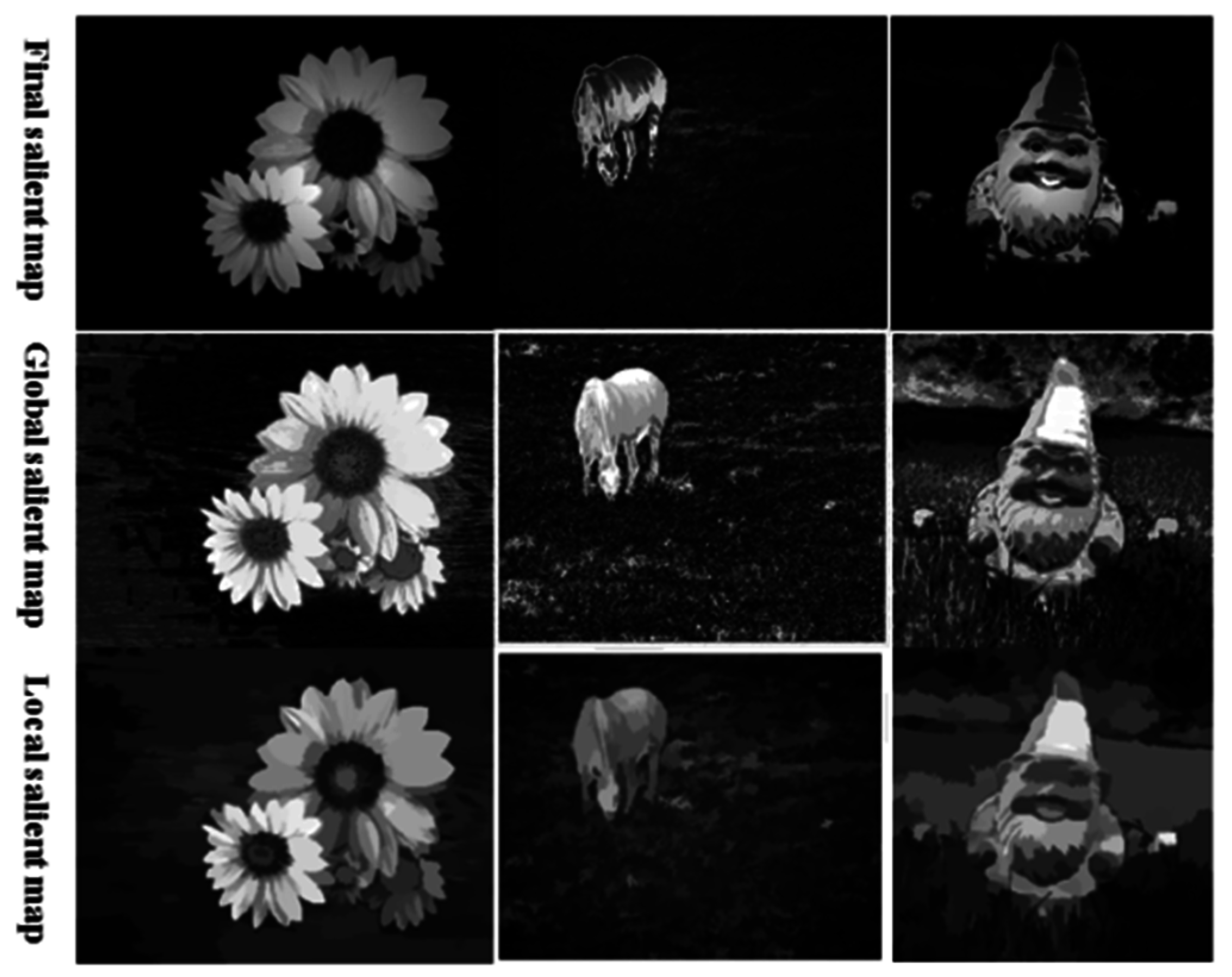
We can clearly observe in Figure 9 that the combined result is better than the global saliency, which is produced from the global color or the salient map obtaining from the region contrast by LTRSH.

Figure 9. The combined result compared with the saliency obtained by LTRSH and global saliency; from top to bottom: the final combined result, global saliency produced using the global color, and saliency obtained by LTRSH.

Figure 9. The combined result compared with the saliency obtained by LTRSH and global saliency; from top to bottom: the final combined result, global saliency produced using the global color, and saliency obtained by LTRSH.

3.5. Final Saliency Enhancement

Then, we further introduce saliency enhancement using the saliency distribution in the global image because when saliency objects/regions are farther from the center of saliency, their saliency is weaker, and vice versa [10]. To solve for this enhancement, we should first determine the center of saliency, and the center position of the salient object/region is defined as the following:

$$Sa{l}_S(\text{center})={\displaystyle \sum _{i=1}^{n}Sal(p_i)Spa(p_i)}/{\displaystyle \sum _{i=1}^{n}Sal(p_i)}$$

(10)

where $Sal(p_i)$ is the saliency of point $p_i$ and $Spa\text{(}{p}_i)$ is the spatial position of point $p_i$. Then, we enhance the saliency at the pixel level to obtain the final saliency of each pixel, which is expressed by Equation (11):

$$Sa{l}_F(p_i)=Sal(p_i)\text{exp}(-\frac{D(p_i,Sa{l}_S(\text{center}))}{\mathsf{\tau }dig})$$

(11)

In Equation (11), $D(p_i,Sa{l}_S(\text{center}))$ is the distance between point $p_i$ and $Sa{l}_S(\text{center})$, $\mathsf{\tau }$ is given as 0.4, and $dig$ is the image diagonal.

4. Experimental Results

We quantitatively validate the effectiveness of our proposed method in saliency detection with the ground truth and five state-of-art salient object/region detection methods’ performance on benchmark datasets [7].

4.1. Datasets and Quantitative Comparison Criterion

The public dataset MSRA-1000 includes 1000 source images and 1000 corresponding manually generated binary ground truth images. The datasets have been widely utilized in the evaluation of salient object detection recently.

In the process of evaluation, we first use Precision and Recall as the evaluated criteria. They are defined as follows:

$$Precision=\frac{{\displaystyle \sum _{i=1}^h{\displaystyle \sum _{j=1}^{w}S(i,j)G(i,j)}}}{{\displaystyle \sum _{i=1}^h{\displaystyle \sum _{j=1}^{w}S(i,j)}}}$$

(12)

$$Recall=\frac{{\displaystyle \sum _{i=1}^h{\displaystyle \sum _{j=1}^{w}S(i,j)G(i,j)}}}{{\displaystyle \sum _{i=1}^h{\displaystyle \sum _{j=1}^{w}G(i,j)}}}$$

(13)

where $S(i,j)$ is the binary gray value converted from the final salient map, $G(i,j)$ is the corresponding ground truth, and h and w are the height and width of the image, respectively.

In addition, the $F_{\mathsf{\beta }}$-measure and mean absolute error (MAE) are then evaluated as they have become increasingly popular in recent years. They are defined as follows:

$$F_{\mathsf{\beta }}=\frac{(1+{\mathsf{\beta }}^2)Precision\times Recall}{{\mathsf{\beta }}^2\times Precision\text{+}Recall}$$

(14)

$$\text{MAE}=\frac{1}{h\times w}{\displaystyle \sum _{i=1}^h{\displaystyle \sum _{j=1}^w\left|Sal(i,j)-G(i,j)\right|}}$$

(15)

where ${\mathsf{\beta }}^2$ is set to 0.3 as usual [7,9], $Sal(i,j)$ is the saliency of each pixel, and $\left|Sal(i,j)-G(i,j)\right|$ is the distance between each pixel’s $Sal(i,j)$ and the corresponding ground truth.

4.2. Performance Evaluation.

Firstly, we use a fixed threshold, which ranges from 0 to 255, to produce the binary object masks on the saliency maps and compute the precision rate and recall rate with the corresponding ground truth masks using Equations (12) and (13). Then, we determine the Precision-Recall curves of our method compared with the other five methods, all of which are shown in following Figure 10.

We can clearly see in Figure 10 that the performance of our method is significantly better than that of the FASA method [6]. The precision of our method always remains above 90% when the recall ranges from 0 to 70%. Our method is better than the RC method when the recall rate of RC remains between 0 and approximately 87%, and they are not much different when the recall is between 87% and 100%. Compared with the SF method, our method’s precision is always higher for recall rates ranging from 0 to 72%, after which our method’s precision begins to slightly decrease for recalls between 72% and 100%.

Figure 10. Precision-recall curves of our method compared with the other five methods.

Figure 10. Precision-recall curves of our method compared with the other five methods.

Secondly, we evaluate our method based on the adaptive threshold [7] by binarizing the salient maps. The mean saliency of the salient map is illustrated as follows:

$$Sa{l}_{mean}=\frac{2}{h\times w}{\displaystyle \sum _{i=1}^h{\displaystyle \sum _{j=1}^{w}Sal(i,j)}}$$

(16)

We calculate the average precision, the average recall and the average $F_{\mathsf{\beta }}$-measure as the overall performance, and then compare with the corresponding ground truth binary masks obtained using the same adaptive threshold. The performance results are shown in Figure 11 and Table 1. The average precision of our method is 89.07%, and the average recall and $F_{\mathsf{\beta }}$-measure are 72.65% and 83.17%, respectively. The following figure and table clearly show that the performance of our method is much better than that of the other methods.

Figure 11. The average Precision, Recall and F-measure based on the adaptive threshold.

Figure 11. The average Precision, Recall and F-measure based on the adaptive threshold.

Table 1. Average precision, recall and F-measure.

Method	Average Precision	Average Recall	Average F-measure
RC	0.882109	0.598936	0.717257
HC	0.742677	0.732207	0.715192
FT	0.748497	0.591377	0.667423
FASA	0.844401	0.743692	0.796570
SF	0.884026	0.741832	0.830650
Ours	0.890686	0.726538	0.831714

Table 1. Average precision, recall and F-measure.

Method	Average Precision	Average Recall	Average F-measure
RC	0.882109	0.598936	0.717257
HC	0.742677	0.732207	0.715192
FT	0.748497	0.591377	0.667423
FASA	0.844401	0.743692	0.796570
SF	0.884026	0.741832	0.830650
Ours	0.890686	0.726538	0.831714

Additionally, we calculate the MAE between the salient maps and the binary ground truth based on Equation (15). The result is shown in Table 2 and Figure 12.

Table 2. The Mean absolute error to ground truth.

Method	RC	HC	FT	FASA	SF	Ours
Mean absolute error	0.2381	0.1749	0.2056	0.1474	0.1309	0.1417

Table 2. The Mean absolute error to ground truth.

Method	RC	HC	FT	FASA	SF	Ours
Mean absolute error	0.2381	0.1749	0.2056	0.1474	0.1309	0.1417

Table 2 shows that our method’s MAE, which is 14.17%, is the second lowest among the six methods. This error is only higher than that of the SF method by approximately 1.07%, and it is lower than that of the FAST method by approximately 0.57%. The MAE rate of RC is 23.81%, which is almost twice that of our method. Therefore, our method is found to perform well when considering the much lower relative MAE.

Figure 12. Mean absolute error to ground truth.

Figure 12. Mean absolute error to ground truth.

Moreover, we compared the average time taken by each method on a Dual Core 2.3 GHz machine with 8 GB of RAM. The execution time of our method implemented in C++ for producing one salient map on MSRA-1000 datasets was estimated as approximately 5.63 s on average. For the other five state-of-art methods, namely RC, HC, FT, FASA and SF, we used the authors’ implementations in C++. Although our method is slower than FASA (0.028 s) and slightly slower than SF (5.23 s) and RC (5.20 s), the saliency detection accuracy is improved in our method, and the time consumed for processing is acceptable. Note that most of the time is consumed in the LTSCH building step, such as texture feature extraction and superpixels segmentation. The time required for each step of our method is shown in Table 3.

Table 3. The time required for each step of our method on average.

Step	Texture Feature Extraction	Superpixels Segmentation	Region Building	Region Contrast Computing	Saliency Enhancement	Global Saliency Computing
Time (s)	1.43	2.70	0.045	1.42	0.015	0.028

Table 3. The time required for each step of our method on average.

Step	Texture Feature Extraction	Superpixels Segmentation	Region Building	Region Contrast Computing	Saliency Enhancement	Global Saliency Computing
Time (s)	1.43	2.70	0.045	1.42	0.015	0.028

Finally, let us present some examples of visual comparison results in Figure 13.

Figure 13. Visual comparison of the six methods on the MSRA-1000 datasets.

Figure 13. Visual comparison of the six methods on the MSRA-1000 datasets.

The above figure clearly shows that the salient maps of our method are visually much better than those of the other methods with full resolution. Our method can not only successfully highlight the salient object/region and uniformly differentiate them from the complex background, but also functions on salient maps with inherent contour and local texture. For instance, take the original horse image in the third line: in our method, the salient object “horse” produced is clearly of better quality, without grassland, and the horse’s mane and the other characteristics are clearly shown. Although the SF method can properly detect the horse with complete contour information in the grassland scene, the detailed characteristics of the horse have poor salient features. Meanwhile, the horse in the salient map using the FASA method is not clearly distinct from the grassland. The salient map of the RC method is not at full resolution. Therefore, the results of our method visually satisfy the criteria introduced in Section 1.

5. Conclusions

In this paper, we present a salient object/region detection method that addresses local texture information, global color information, and spatial layout to produce full-resolution salient maps with detailed inherent shape and local texture information for the salient object/region. Although much better salient maps with intact contour and local texture information of the salient object/region are ensured by the effectiveness of FASA’s computation of global saliency probability, but greatly benefit from our proposed LTRSH model. As our main contributions, LTRSH combines the advantages of local texture and color statistical information with contour information to effectively describe the local region character information of the image. Moreover, the experimental results demonstrate that our proposed method obtains better performance when compared to five state-of-the-art methods. In the future, we plan to improve the model LTRSH’s efficiency, as some sub-steps are currently the most time-consuming steps in our salient object/region detection method. We will also investigate the use of salient maps as prior knowledge for image segmentation, even for high-level applications such as image classification and annotation.