Prediction of Experimental Rainfall-Eroded Soil Area Based on S-Shaped Growth Curve Model Framework

Abstract

Rainfall-induced soil erosion of a mountain area plays a significant role in supplying sediment and shaping the landscape. The related area of soil erosion, as an index of the changed landscape, is easier to calculate visually using some popular imaging tools. By image analysis, our work shows that the changing of the soil erosion area admits the structure of an S-growth curve. Therefore, we propose to establish an S-curve model, based on incremental learning, to predict the soil erosion area. In the process of incremental learning, we dynamically update the accumulative rainfall and rainfall intensity to train the parameters of our S-curve model. In order to verify our prediction model, the index of area is utilized to express the output of eroded soil in a series of experiments. The results show that the proposed S-growth curve model can be used to estimate the growth of the soil erosion area (average relative error 3%–9.7%) according to variable soil material and rainfall intensity. The original S-growth curve model can calculate the erosion areas of just one soil material and one rainfall condition whose average relative error is 7.5%–12.2%; compared to the simple time series analysis-moving average method (average relative error 5.7%–12.1%), our proposed S-growth curve model can reveal the physical mechanism and evolution of the research object.

1. Introduction

Rainfall-induced soil erosion involves three main processes: detachment, transport, and deposition of soil particles by the crush forces of rainfall and surface runoff. During the erosion process, the area of soil erosion can reflect the shaped landscape. The classical estimation models of soil erosion include the USLE model, which is composed of six factors to predict the long-term average annual soil weight [1,2]; the WEPP model, which is capable of predicting spatial and temporal distributions of soil detachment and deposition on an event or continuous basis at both small (hillslopes, roads, small parcels) and large (watershed) scales [3]; the EUROSEM model, which is a dynamic distributed model, able to simulate sediment transport, erosion and deposition by rill and inter-rill processes in single storms for both individual fields and small catchments [4]; the KINEROS model, which is an event-oriented, physically-based model describing the processes of interception, infiltration, surface runoff and erosion from agricultural and urban watersheds [5]. These models can commonly describe the distributions of soil detachment in large (watershed) scales. By contrast, in our study, a narrow scale of even a single slope is our research object. We aim to investigate the development of the area of soil erosion induced by rainfall in a single slope using an imaging tool. In the practical experiments, the values of rainfall intensity and cumulative rainfall are acquired incrementally with respect to time. The area of soil erosion is achieved by the imaging tool under time domains. Then, in this work, based on incremental learning, we develop an S-curve model to predict the soil erosion area. In detail, we update the input values chronologically to train the parameters of the S-curve model. Five experiments involving different materials and different rainfall intensities are employed to validate the model.

2. Physical Experiments and Results

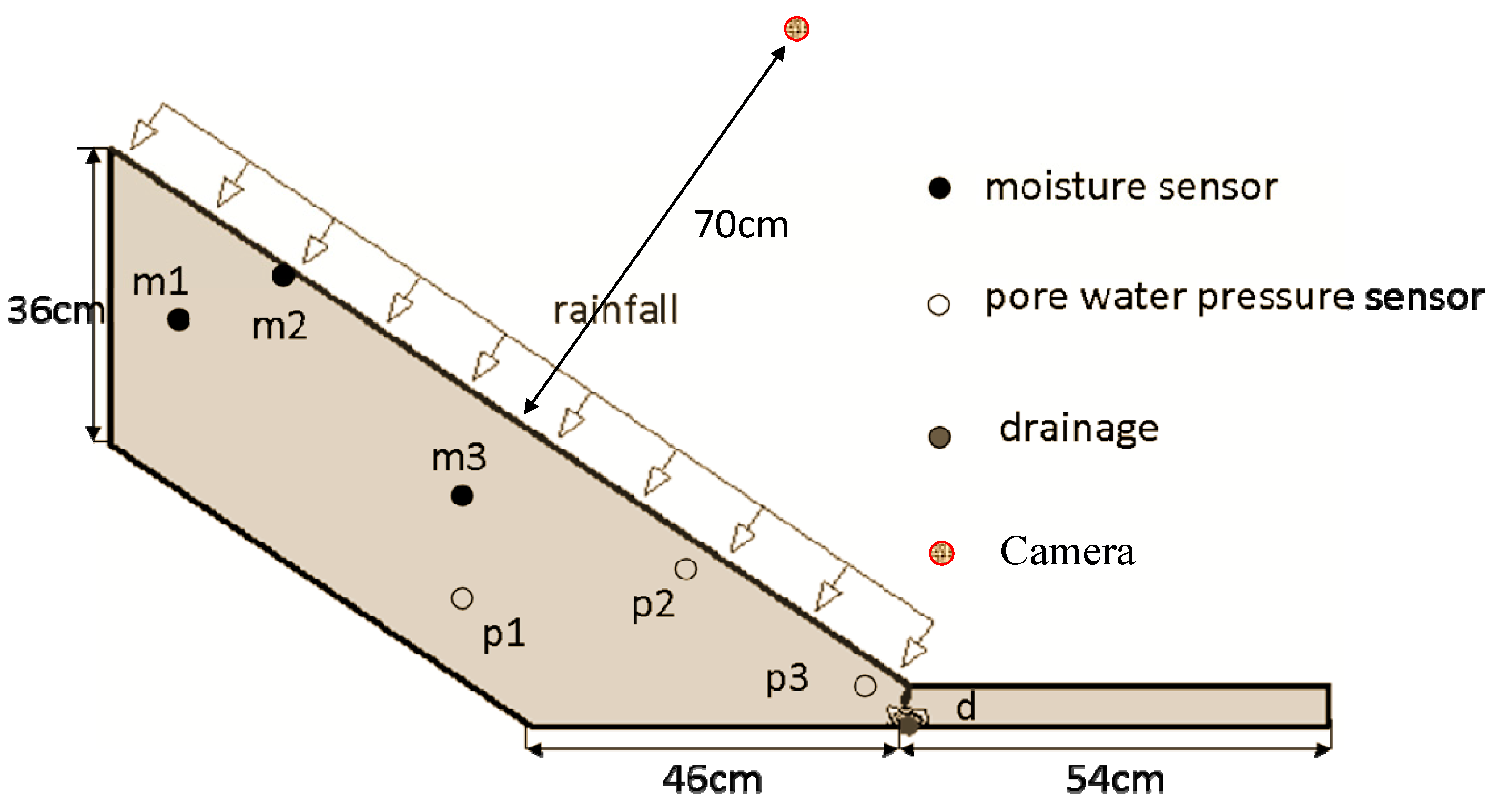
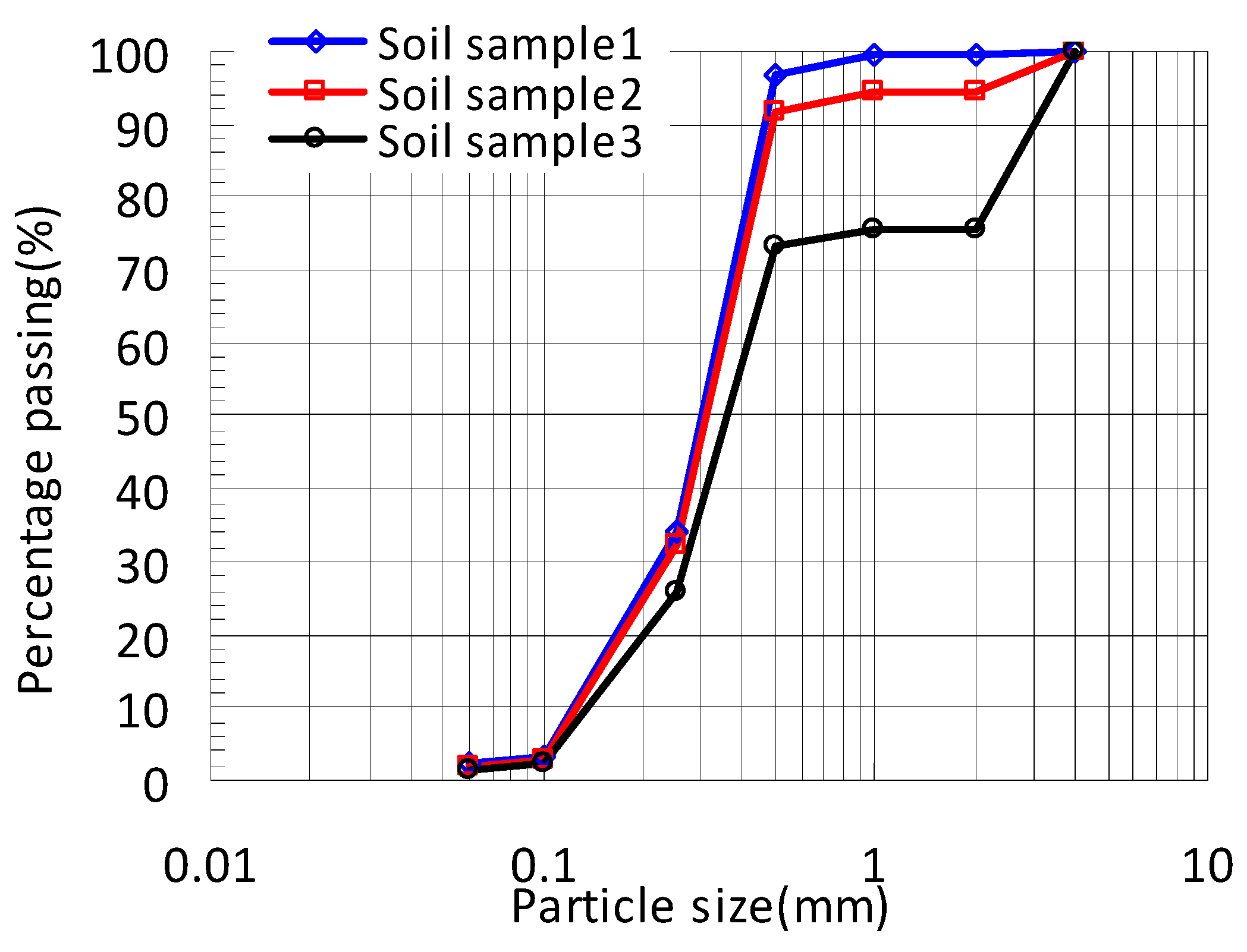
2.1. Physical Models, Monitoring Devices, and Experimental Procedures

Schmidt et al. [6] highlight the advantage of physically-based models: using minimal historical data to produce meaningful results. Thus, a trend of developing and testing physically-based soil erosion models appears [7,8,9,10,11]. In our study, a slope model is constructed in a flume device made of Plexiglas (Figure 1). The slope inclination is 34° and the material is from Fengdu Mountain, near to Yangtze River Bank, Chongqing, China, whose surface soil can be easily eroded under heavy rainfall. The soil was air-dried and crushed to different test samples having three particle size distributions, as shown in Figure 2. The soil sample was squeezed by a plate with a 120 N force to form the slope. In order to reduce the “boundary effect”, we used a covering of polytetrafluoroethylene (PTFE) whose friction coefficient is 0.04 on both sides of the flume. In Figure 1, m is the moisture transducer (frequency domain sensor) [12] whose contact area with the soil is less than 20 mm² (measuring range 0%–100%, resolution 0.1%, deviation ±2%); p is the pore water pressure transducer (diameter 3 cm, height 1.6 cm, measuring range ±10 kPa, deviation ±0.2%); d is a channel for drainage; one high-definition digital video camera (5 million pixels, position in Figure 1) is used to record the changes of the eroded soil area (front scene). Every test is conducted under similar initial geometry, and pre-added water content (deviation ±3%, average value ~5.2%). Persistent rainfall is averagely simulated by three nozzle spray heads (~0.6 m high to slope surface) in five rainfall events. For soil Sample 1, we used three rainfall intensity levels in three experiments (approximately 25, 45, and 65 mm/h, respectively) to investigate the effect of different rainfall intensities on the same material. Then we focused on the effect of the different materials (Sample 1, Sample 2, and Sample 3), by comparing their responses in experiments with a common rainfall intensity of 45 mm/h.

Figure 1. Geometry of physical model.

Figure 1. Geometry of physical model.

Figure 2. Particle-size distribution curves.

Figure 2. Particle-size distribution curves.

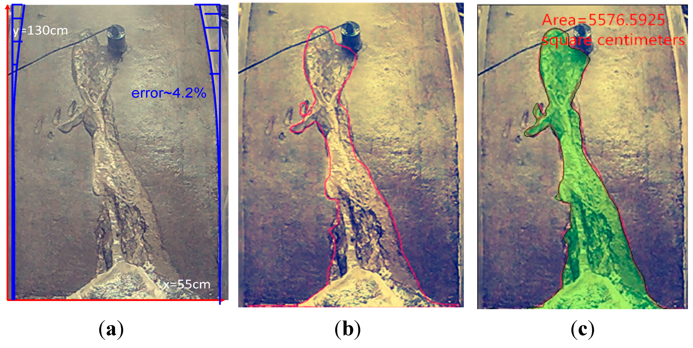
2.2. Soil Erosion Area Calculation

A fast way to calculate a two-dimensional area of an object is to use the “BOUNDARY” command in the AutoCAD software (Autodesk, Inc., San Rafael, CA, United States of America) [13]. Using “BOUNDARY”, a point can be picked within the area to create a closed poly line or polygon domain. The “Features” palette can be used to find the area and perimeter of the poly line or polygon domain. By using the “MEASUREGEOM” and “AREA” commands, a series of points or a selected object is specified to calculate the area. In Figure 3a, a coordinate is first established. Then the contour of the eroded soil area is extracted in Figure 3b. Finally, in Figure 3c, calculation of the selected area is executed by AutoCAD. In every experiment, the video data per minute is chronologically intercepted to calculate the area. Lens distortions and the distance between camera and ground affect the accuracy of the picture area. An error calculation is carried out in Figure 3a, and it is found that the blue part, which concentrates on the upper part is a picture area error of ~4.2%, while most of the soil erosion happens in the lower part, which means that the area error of soil erosion could be less than 4.2%.

Figure 3. Area calculation by AutoCAD (soil Sample 1 and rainfall intensity-65 mm/h): (a) establishment of coordinate; (b) extraction of contour; and (c) calculation of areas.

Figure 3. Area calculation by AutoCAD (soil Sample 1 and rainfall intensity-65 mm/h): (a) establishment of coordinate; (b) extraction of contour; and (c) calculation of areas.

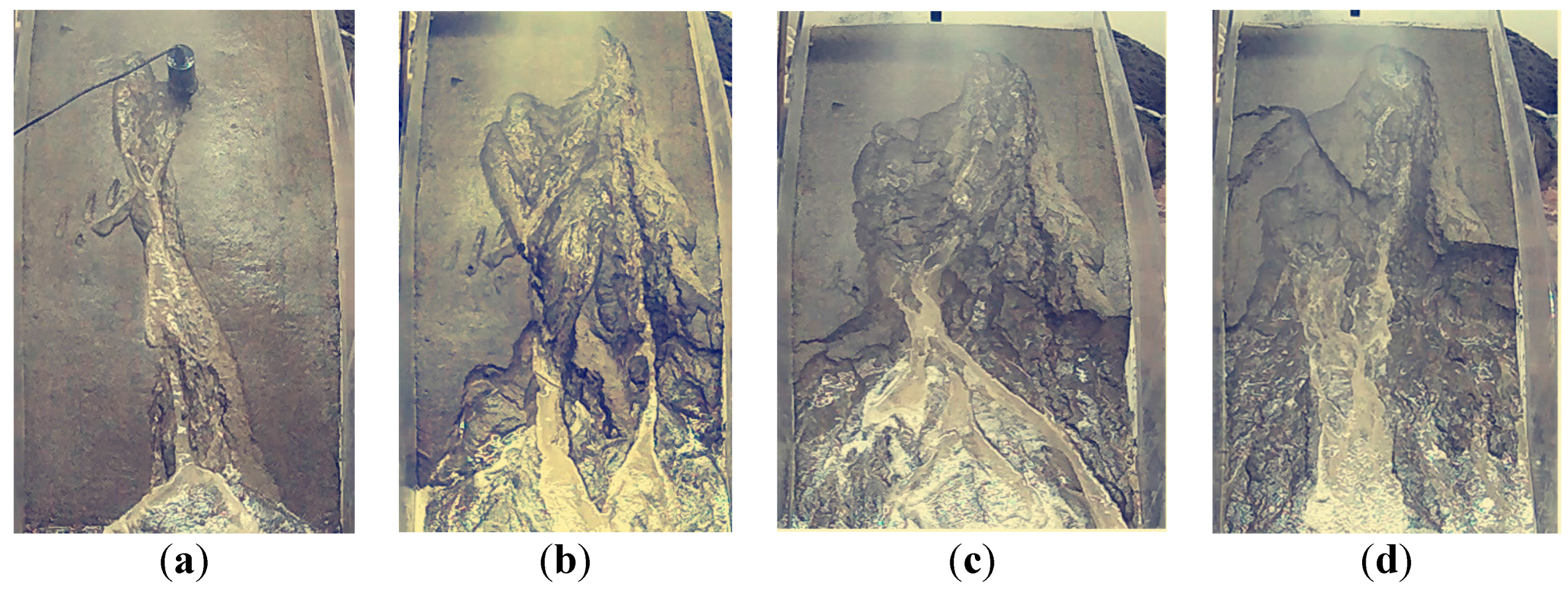
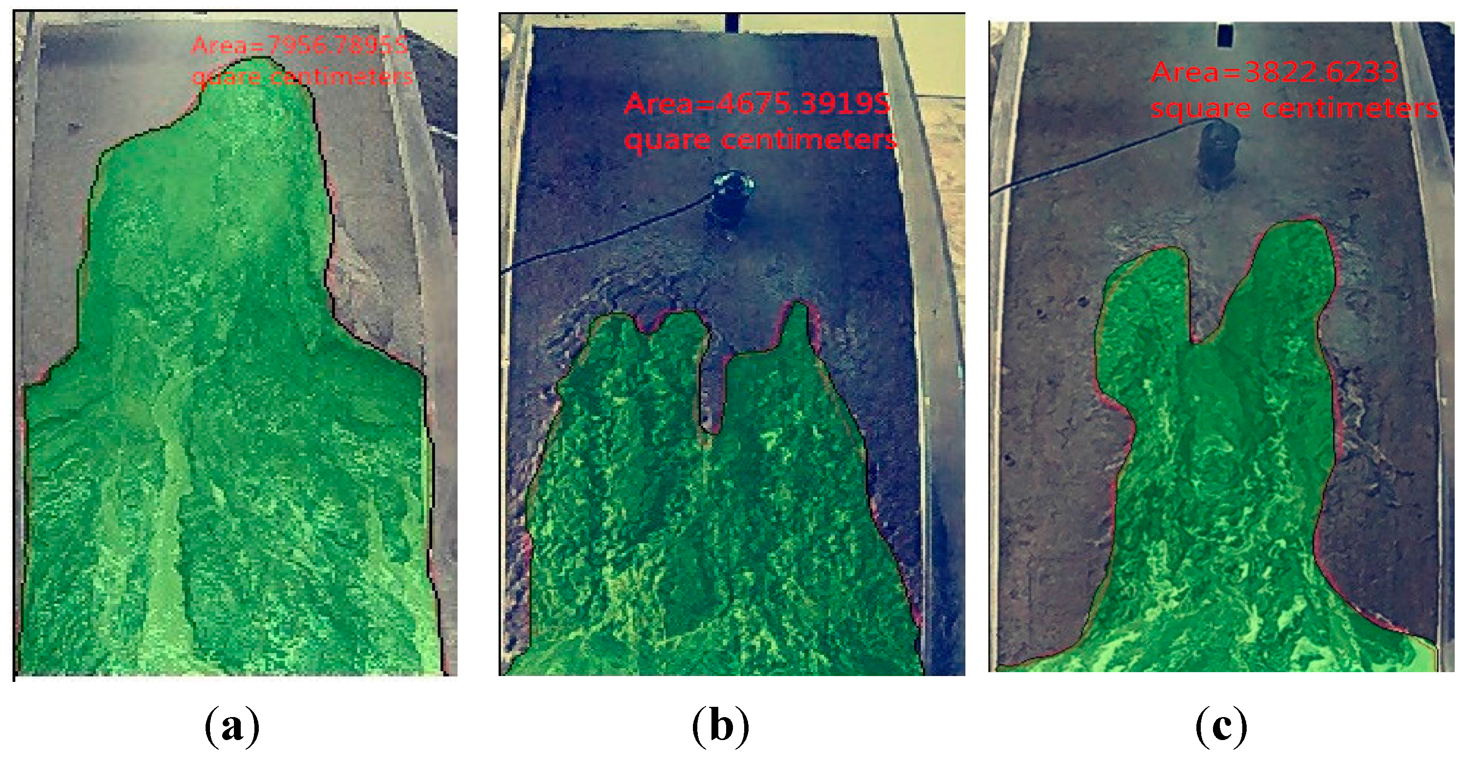
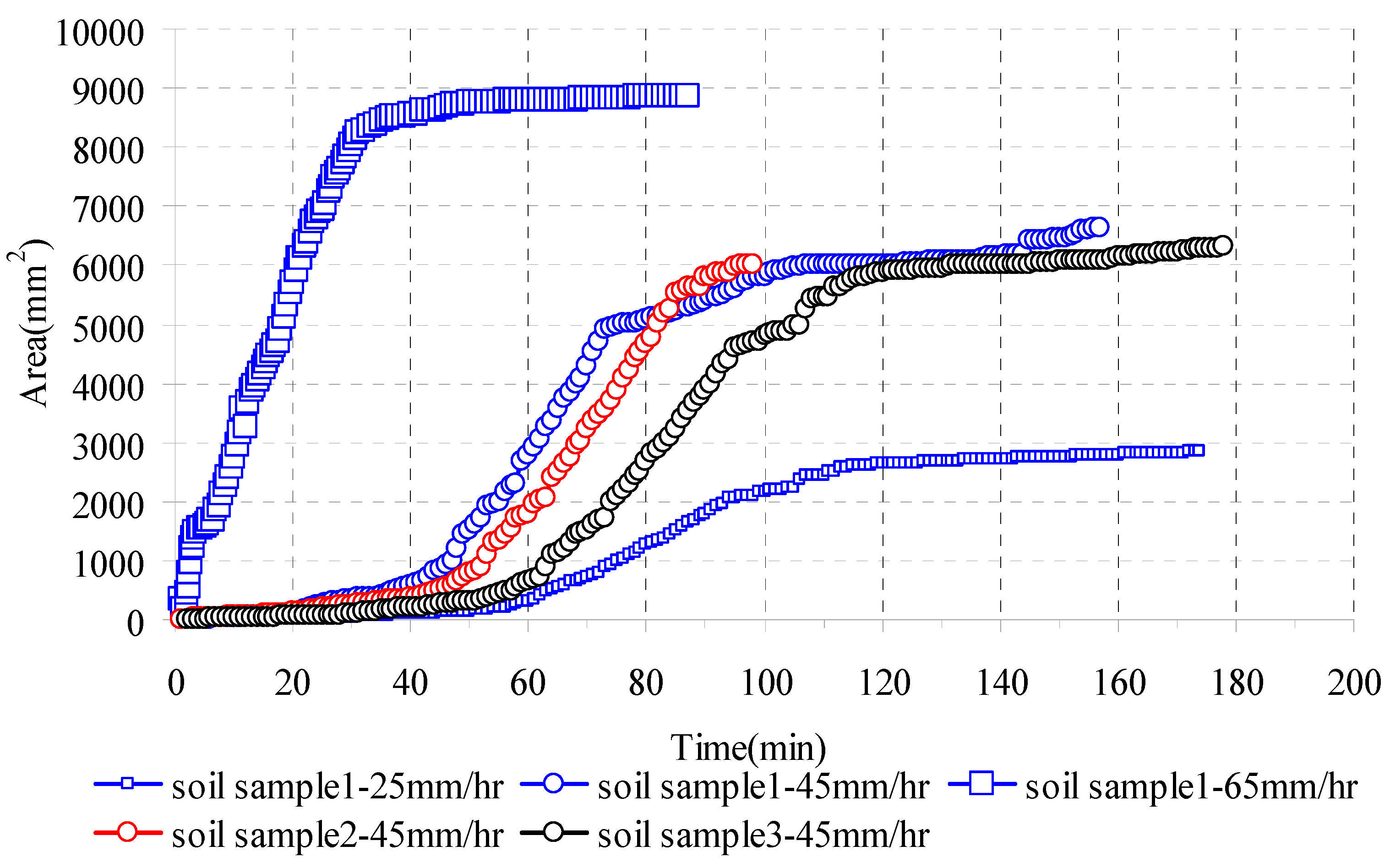
2.3. Soil Erosion Area

Increased detachability produced by surface runoff shear forces and the impact of raindrops is considered as the main force driving erosion [14]. Figure 4 illustrates that the toe of the slope is more eroded than other positions, in consideration of more ground water supply from the upper parts. The erosion of the top part of the slope without ground water supply from other parts shows a slow increase. Thus, this is typical progressive soil erosion. Figure 5 shows the erosion of different materials under the same time domain and rainfall intensity. It is found that the coarse particles (such as soil Sample 3) have lower erosion than fine particles (such as soil Sample 1) because of their higher permeability and stronger framework.

Figure 4. Different time domains in Sample 1 and rainfall intensity-65 mm/h test: (a) t = 6 min; (b) t = 19 min; (c) t = 45 min; and (d) t = 70 min.

Figure 4. Different time domains in Sample 1 and rainfall intensity-65 mm/h test: (a) t = 6 min; (b) t = 19 min; (c) t = 45 min; and (d) t = 70 min.

Figure 5. Different materials under the same time domain (45 mm/h; t = 52 min): (a) soil Sample 1 and erosion area-771.21 mm²; (b) soil Sample 2 and erosion area-421.31 mm²; (c) soil Sample 3 and erosion area-359.46 mm².

Figure 5. Different materials under the same time domain (45 mm/h; t = 52 min): (a) soil Sample 1 and erosion area-771.21 mm²; (b) soil Sample 2 and erosion area-421.31 mm²; (c) soil Sample 3 and erosion area-359.46 mm².

In Figure 6, soil Sample 1 (25 mm/h) has the most obvious initial phase (threshold of soil erosion action) because of the low rainfall intensity. By comparison, soil Sample 1 (45 mm/h) and soil Sample 1 (65 mm/h) have fewer time lags. In the second acceleration stage, the erosion under higher rainfall intensity obviously occurs faster because of the greater surface runoff production. In the last phase, for one thing the coarse particles remain and the loss of fine particles makes the soil structure stronger; for another, the water erosion develops towards the deep direction. Therefore, the soil erosion area has a maximum value, but the volume could still increase. By contrast, for different materials, soil Sample 1 (more fine particles), with the weakest structure, has the earliest start point of the second erosion phase and a high erosion rate during the second stage because more surface fine particles are lost. Until the final stage (relatively stable structure), the erosion rate is still higher than for the coarse materials, but only towards the deep direction. For the area of soil erosion in the final stage, the values of the three materials can be close, while for the erosion volume or weight the coarse material has a lower value. This is because coarse particles like soil Sample 3 have a stronger structure (high friction) and higher infiltration rate (producing less surface runoff) than fine particles like soil Sample 1. In addition, it can also be seen that the stronger the structure of coarse material against soil erosion is, the greater is the time lag of the beginning and accomplishment of the erosion area compared to fine material. In summary, the soil erosion is decided by both rainfall and the material’s strength.

Figure 6. Results of soil erosion experiments.

Figure 6. Results of soil erosion experiments.

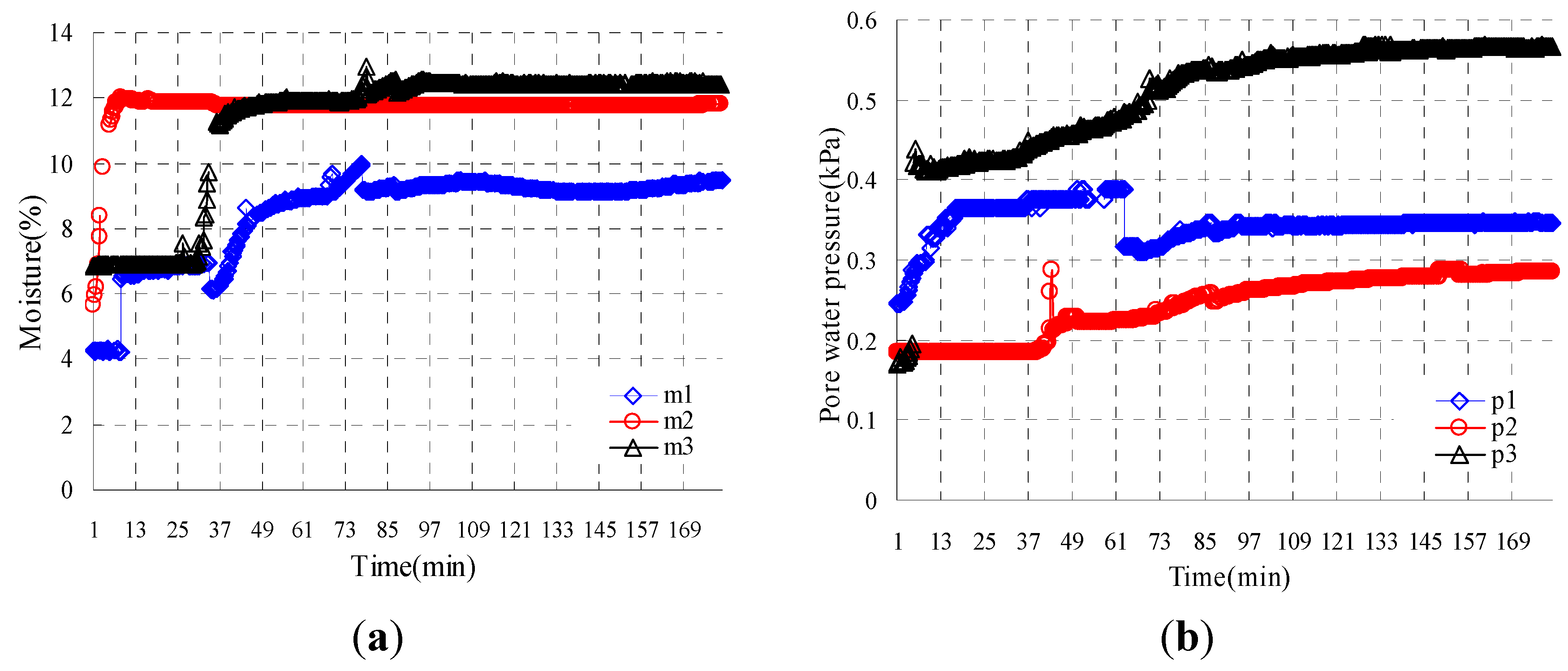
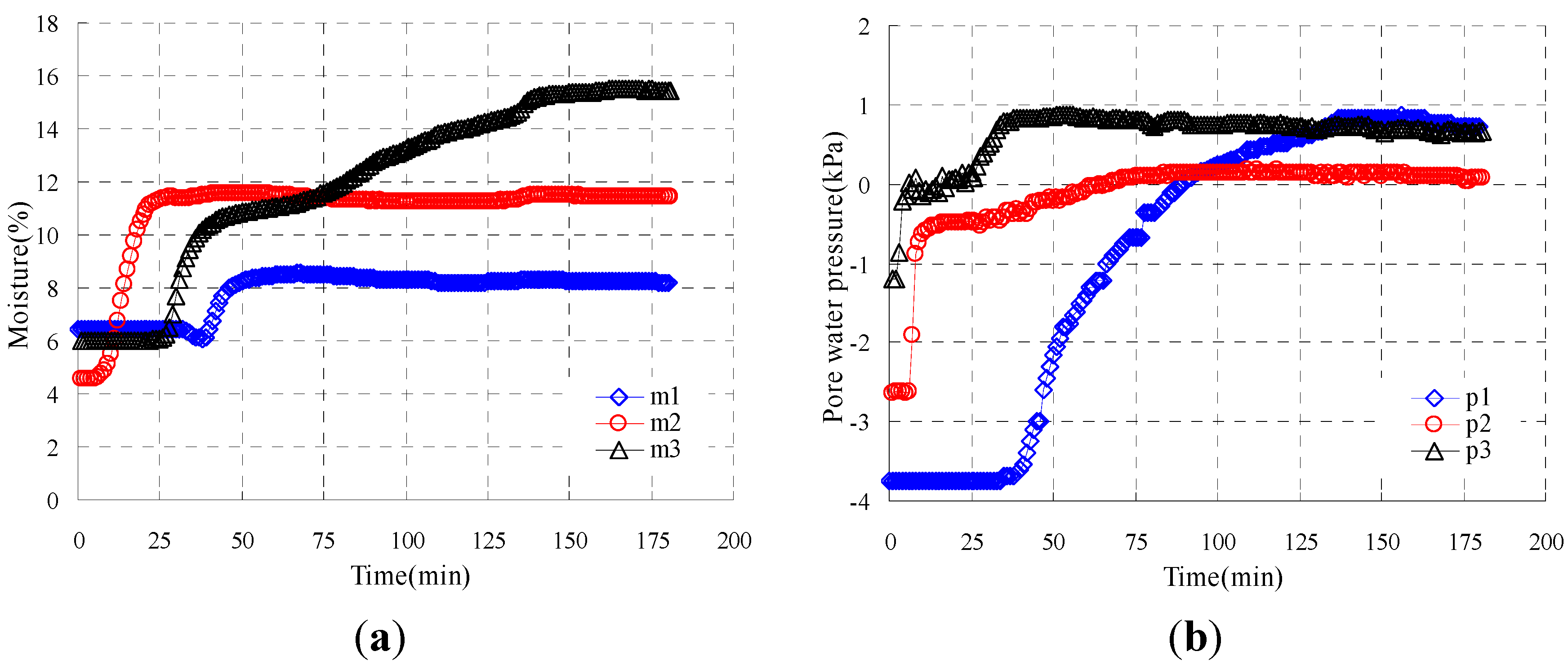
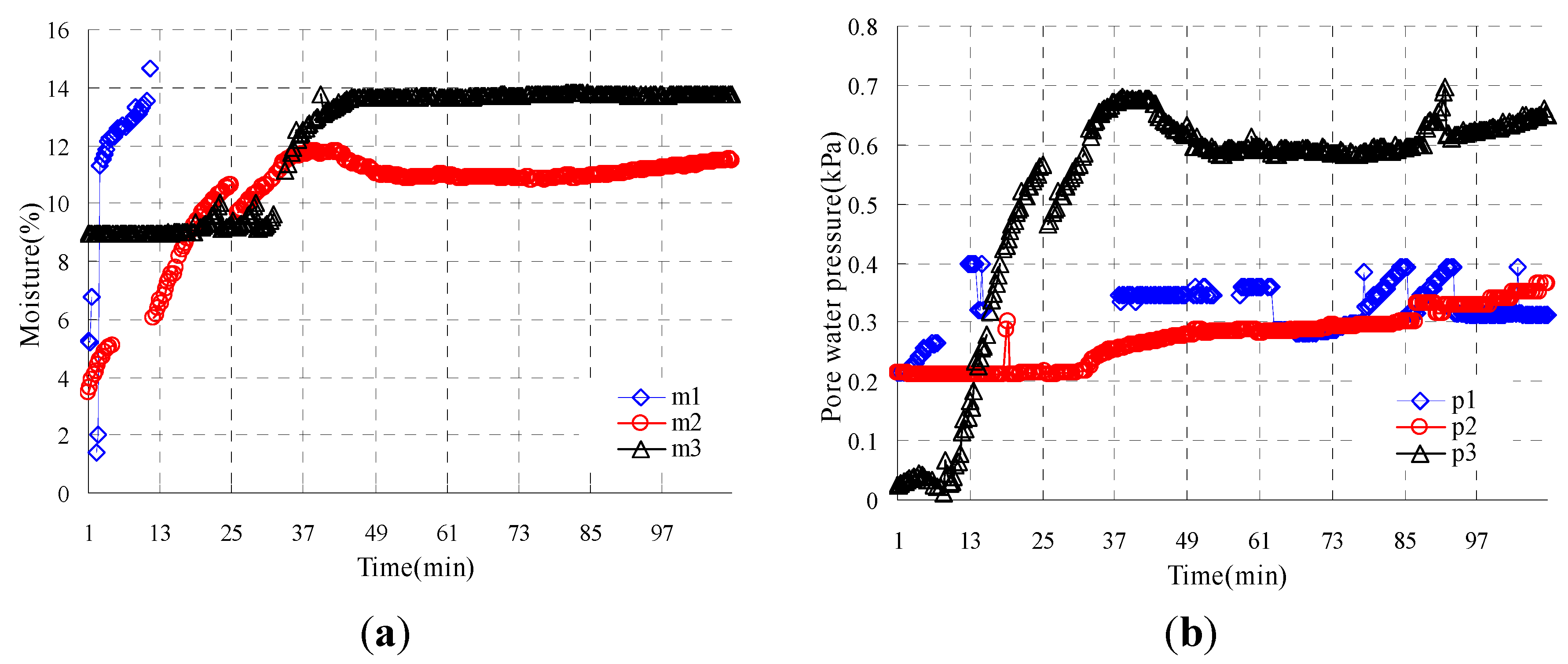
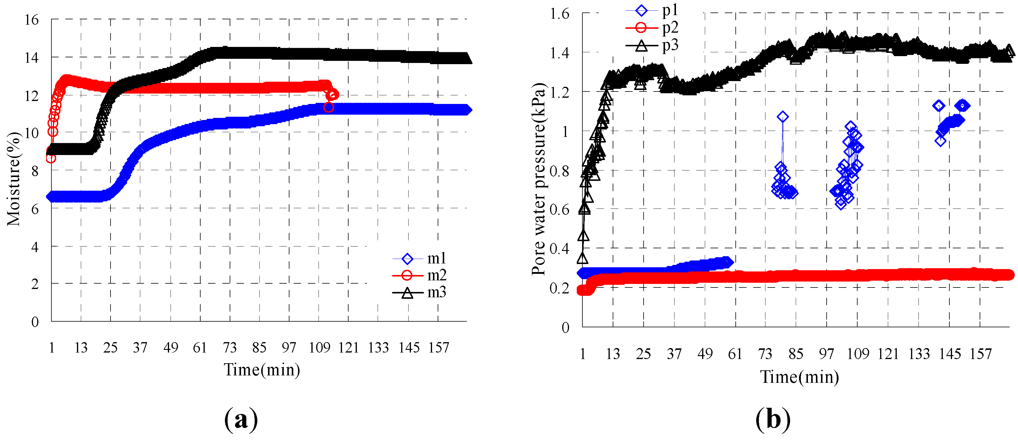
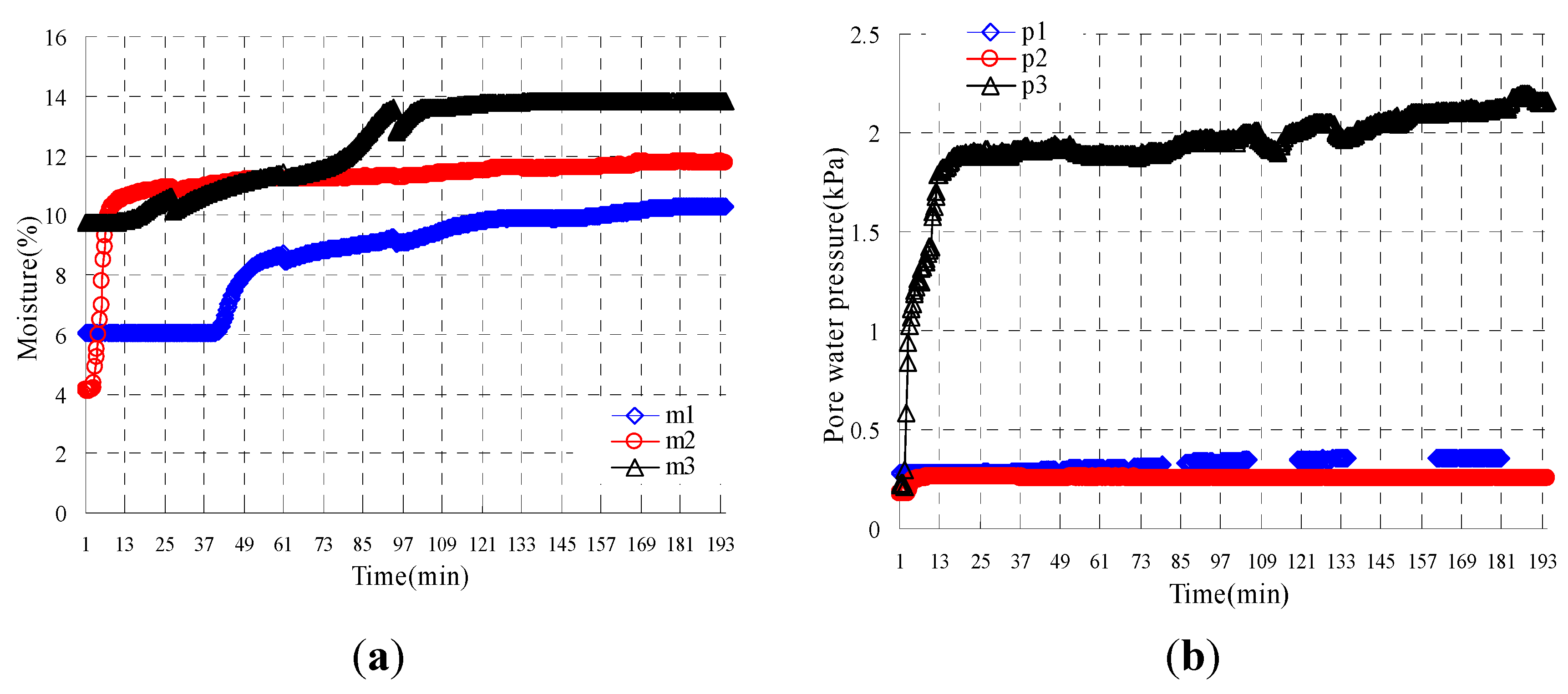
2.4. Hydrological Characteristics

Subsurface water content and soil pore water pressure might reflect the effects of rainfall on the processes of surface sealing, runoff generation and soil sediment production. For one thing, high soil moisture content or low negative pore water pressure results in an increased detachability by surface runoff shear forces and raindrop impact [14]. For another aspect, a high water content of the soil might decrease aggregate slaking and breakdown due to less air escaping upward, reducing the detachment of soil by raindrop impact [15,16]. In Figure 1, m1 is at the middle deep position; m2 is near to the surface; and m3 is at the low part. By contrast, p1 is at the middle depth position; p2 is near to the surface; and p3 is at the toe of the slope. Figure 7a demonstrates that m2 near to the surface increases more easily. Due to their depth, m1 and m3 have a certain time lag before increasing of water content. Furthermore, m3 has a higher value and a shorter time lag because of the water flow supply. In Figure 7b, the pore water pressure follows a similar pattern. Point p2, at the surface, is always saturated to some degree and has no potential to increase. Point p3 has a higher value than p1 because of its deeper position. For the same material, a higher rainfall intensity means more water input. Therefore, m and p have higher values and lower time lags in Figure 8 and Figure 9. For the different materials, in Figure 8, Figure 10 and Figure 11 the coarse particles in soil Sample 3 have higher permeability or a higher infiltration rate than fine particles. Thus, the time lag of pore water pressure production in coarse materials is shorter and the value is higher. The moisture value depends on the balance of the water infiltration, supply, and drainage.

Figure 7. Soil Sample 1-25 mm/h: (a) Moisture content of m1, m2, and m3; and (b) pore water pressure of p1, p2, and p3.

Figure 7. Soil Sample 1-25 mm/h: (a) Moisture content of m1, m2, and m3; and (b) pore water pressure of p1, p2, and p3.

Figure 8. Soil Sample 1-45 mm/h: (a) Moisture content of m1, m2, and m3; and (b) pore water pressure of p1, p2, and p3.

Figure 8. Soil Sample 1-45 mm/h: (a) Moisture content of m1, m2, and m3; and (b) pore water pressure of p1, p2, and p3.

Figure 9. Soil Sample 1-65 mm/h: (a) Moisture content of m1, m2, and m3; and (b) pore water pressure of p1, p2, and p3.

Figure 9. Soil Sample 1-65 mm/h: (a) Moisture content of m1, m2, and m3; and (b) pore water pressure of p1, p2, and p3.

Figure 10. Soil Sample 2-45 mm/h: (a) Moisture content of m1, m2, and m3; and (b) pore water pressure of p1, p2, and p3.

Figure 10. Soil Sample 2-45 mm/h: (a) Moisture content of m1, m2, and m3; and (b) pore water pressure of p1, p2, and p3.

Figure 11. Soil Sample 3-45 mm/h: (a) Moisture content of m1, m2, and m3; and (b) pore water pressure of p1, p2, and p3.

Figure 11. Soil Sample 3-45 mm/h: (a) Moisture content of m1, m2, and m3; and (b) pore water pressure of p1, p2, and p3.

3. Soil Erosion Area Prediction Model

3.1. S-Shaped Growth Curve

The S-curve is one of the most common phenomena in nature: It is seen in the spreading of populations, tumors, contaminants, innovations, and economic activity [17,18,19,20]. The pattern of an S-shaped growth curve (Pearl growth curve) usually comprises three phases in an environment: the object initially increases slowly; then it enters a positive acceleration phase, increasing rapidly and approaching an exponential growth rate as in the J-shaped curve; and finally, the object declines in a negative acceleration phase until reaching almost zero growth rate (logistic function).

$$y=\frac{k}{1+b{e}^{-ax}},a>0,k>0,x>0$$

(1)

As shown in Equation (1), this slowing of the growth rate reflects increasing environmental resistance, which becomes proportionately more important at higher object densities. The point of stabilization, or zero growth rate, is termed the “saturation value” (symbolized by k) or “carrying capacity” of the environment. a and b are the parameters that decide the trend of curve development; y is the output object; and x is the input variable. It is usually summarized mathematically by the logistic equation. In our case, when the cumulative rainfall (x) achieves a certain threshold, erosion begins to occur. Thus, in the first stage, the eroded area (y) increases slowly, even having some time lag, especially under low rainfall intensity; in the second phase, the eroded area increases swiftly due to the shear force produced by surface runoff; in the final phase, because of surface loss of weak particles while strong particles remain, the erosion develops deeper into the slope (“carrying capacity” of the environment (k)), and the eroded area growth rate then begins to reduce, even to zero.

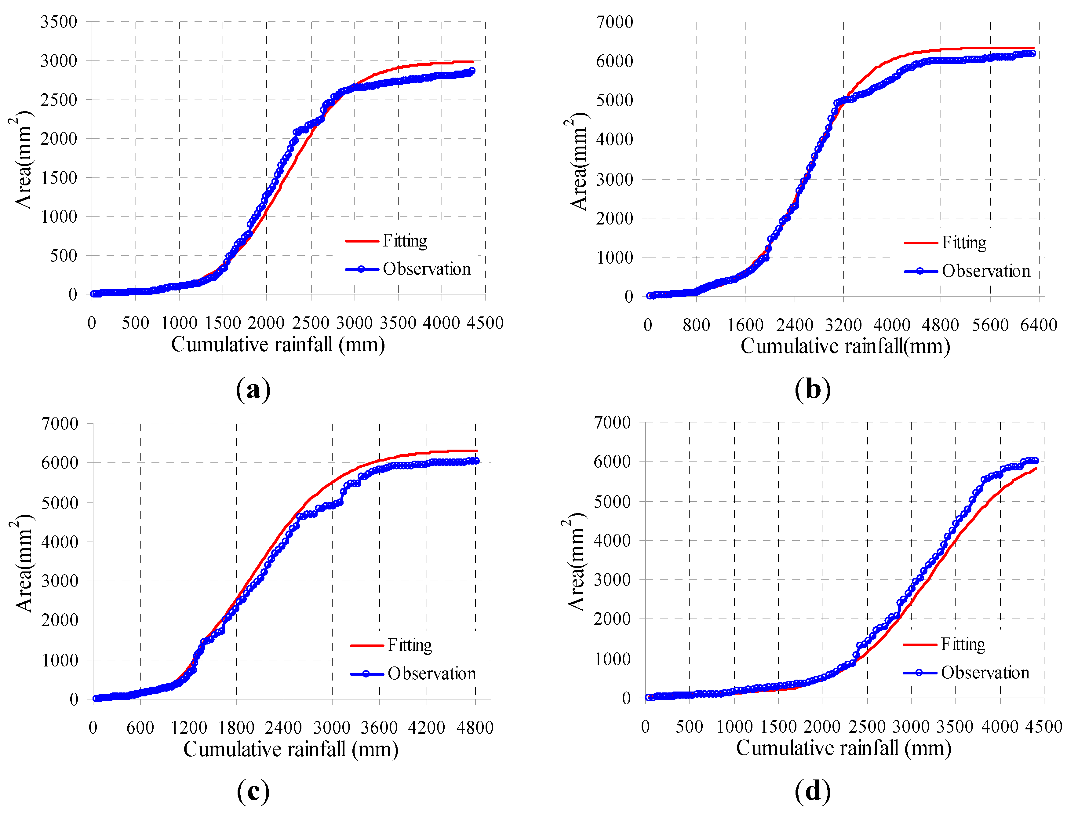
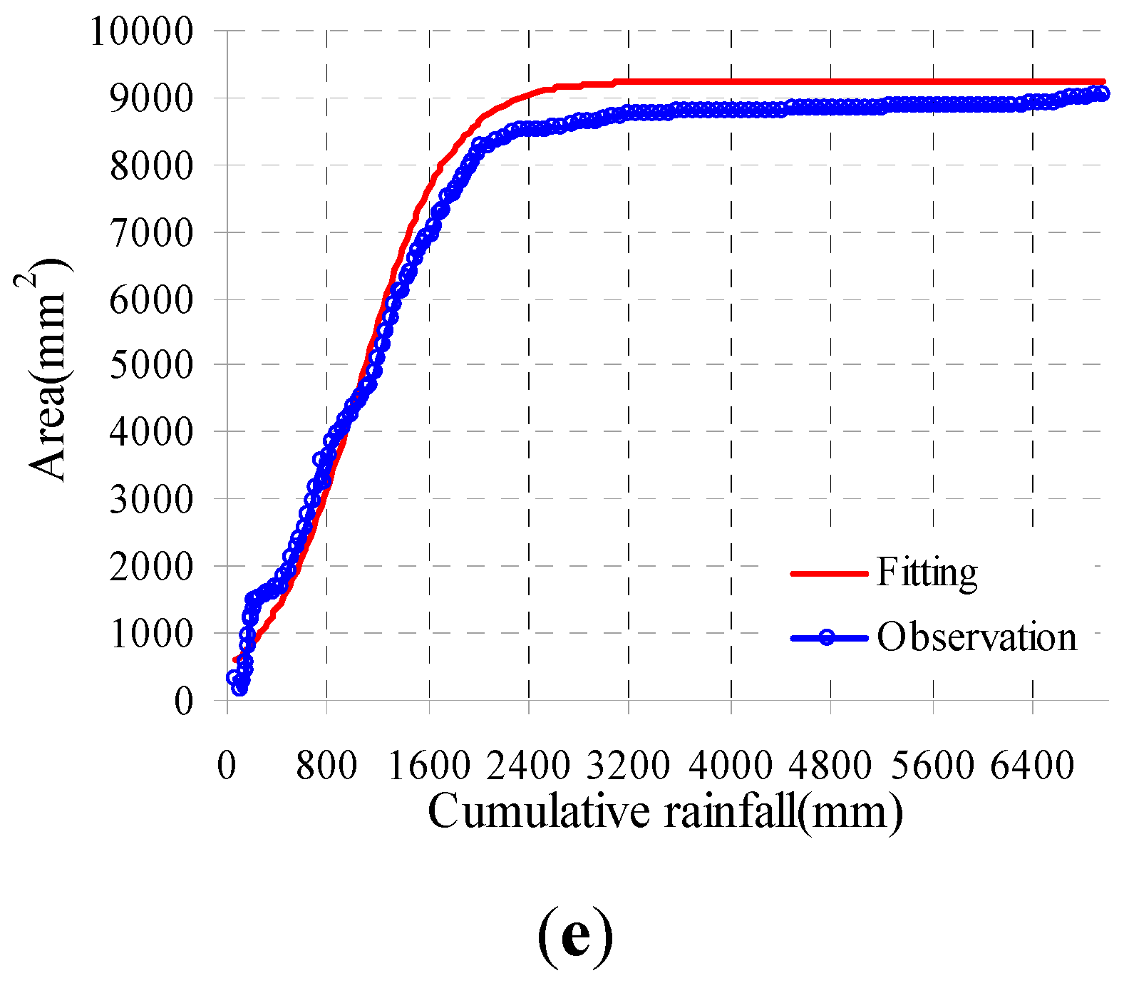
3.2. S-Shaped Growth Curve Fitting

According to Equation (1), the S-curves of the five experiments are fitted. In Equation (1), x is cumulative rainfall; y is the eroded area; k is the maximum eroded area; a is a parameter related with material; and b is a parameter to control the erosion rate. Figure 12 shows that the S-curve model matches the soil erosion area development with a relative average error of 7.5%–12.2%. Table 1 presents the parameters in the five models.

Figure 12. S-growth curve fitting: (a) soil Sample 1-25 mm/h; (b) soil Sample 1-45 mm/h; (c) soil Sample 1-65 mm/h; (d) soil Sample 2-45 mm/h; and (e) soil Sample 3-45 mm/h.

Figure 12. S-growth curve fitting: (a) soil Sample 1-25 mm/h; (b) soil Sample 1-45 mm/h; (c) soil Sample 1-65 mm/h; (d) soil Sample 2-45 mm/h; and (e) soil Sample 3-45 mm/h.

Table 1. Parameters of five S-shaped growth curves.

Name	k	a	b
Soil Sample 1-25 mm/h	3000	1.088 × e4	10.4
Soil Sample 1-45 mm/h	6350	4.75 × e5	15.2
Soil Sample 1-65 mm/h	9250	4.215 × e5	1.176
Soil Sample 2-45 mm/h	6350	4.4 × e5	20.6
Soil Sample 3-45 mm/h	6350	4.267 × e5	16.9

Table 1. Parameters of five S-shaped growth curves.

Name	k	a	b
Soil Sample 1-25 mm/h	3000	1.088 × e4	10.4
Soil Sample 1-45 mm/h	6350	4.75 × e5	15.2
Soil Sample 1-65 mm/h	9250	4.215 × e5	1.176
Soil Sample 2-45 mm/h	6350	4.4 × e5	20.6
Soil Sample 3-45 mm/h	6350	4.267 × e5	16.9

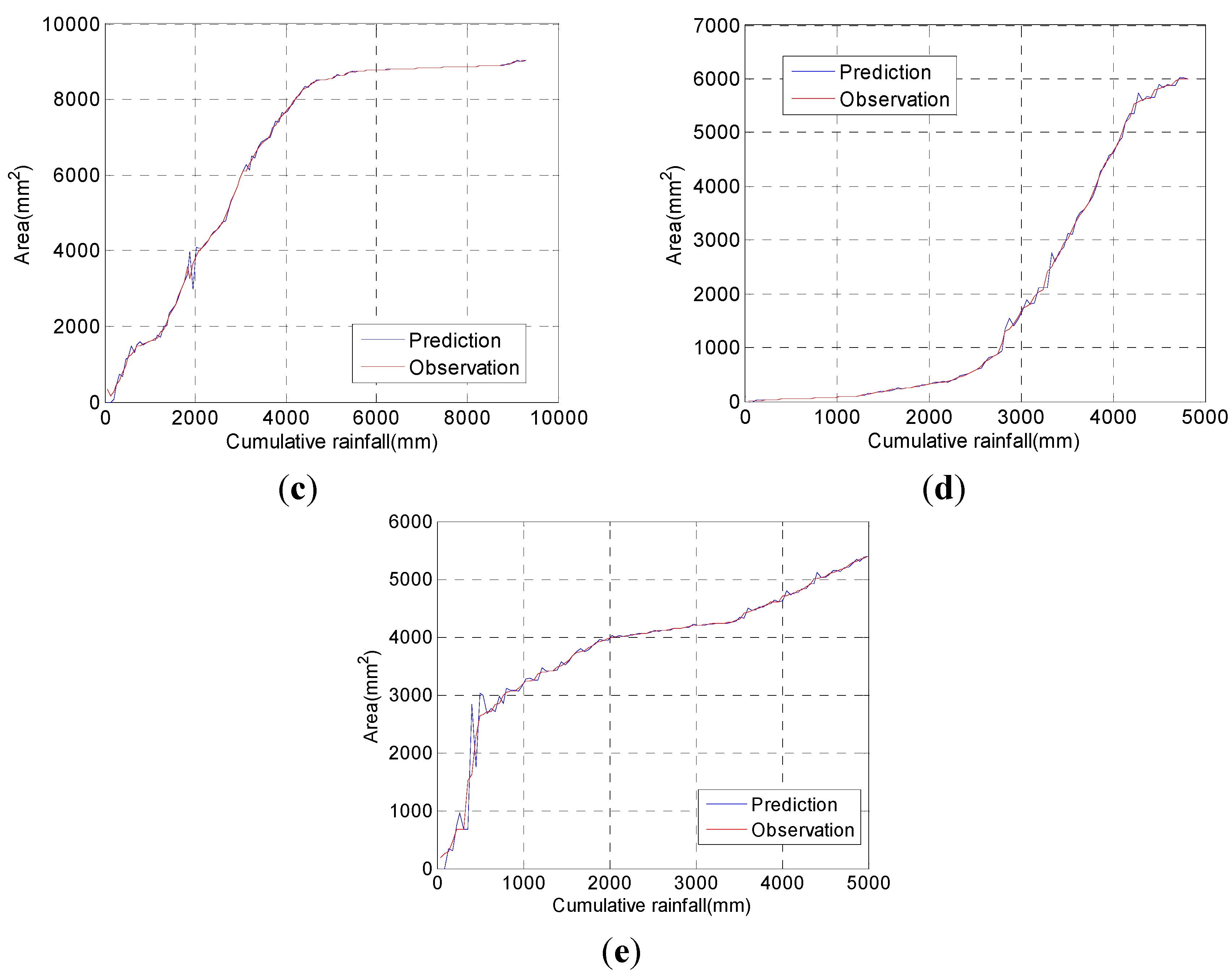
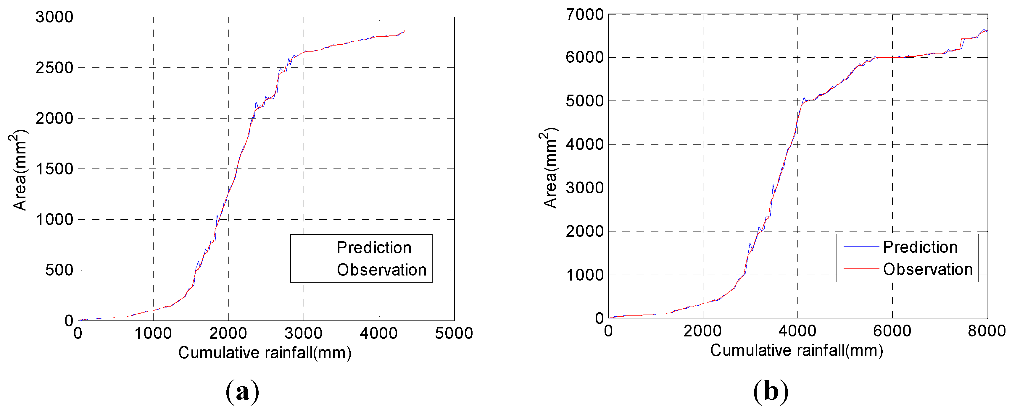
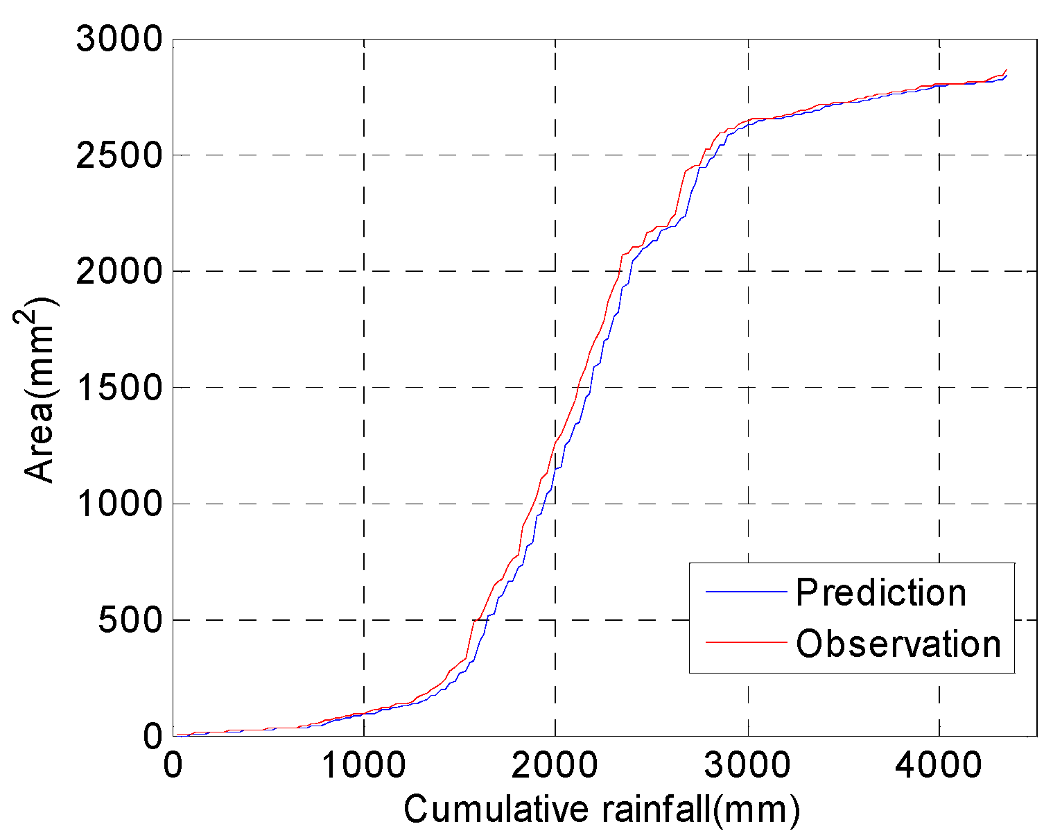
3.3. Development of Prediction Model

In order to predict the S-shaped growth curve framework based on different soil materials under different rainfall intensities, we used the previous observation values to train the parameters of a model to predict the object in the next time domain and then repeat the process in the following time domain, which is similar to the dynamically updated method. The modified S-shaped growth curve framework is used to predict the eroded area $s_{t+\mathrm{1}}$ at time t+1, as in Equation (2):

$$s_{t+\mathrm{1}}=\frac{k\prime }{\mathrm{1}+b_t{e}^{-a_t(x_t-x_{t-\mathrm{1}})}},a_t>0,k\prime >0,b_t>0$$

(2)

where $a_t$, related to material, is the parameter affecting the erosion rate at time t. It is considered a variable as time elapses because the particles of the soil change. $b_t$ is considered as the variable which depends on the cumulative eroded area and rainfall intensity at time t. $x_t$ and $x_{t-\mathrm{1}}$ are the cumulative rainfall at time t and t−1, respectively.

In Equation (1), the initial value of $b_{\mathrm{0}}$ can be calculated when t is zero. Therefore,

$$b_{\mathrm{0}}=(\frac{k\prime }{s_0}-\mathrm{1})$$

(3)

where k’ is the “saturation value” or “carrying capacity” of the eroded area. From the results in Table 1, it is found that k is mainly affected by rainfall intensity m linearly, rather than the material parameter a, which is read as

$$k\prime =\lambda m-\mu ,m>3.44$$

(4)

where m is the rainfall intensity and the coefficients $\lambda$ (147.5) and $\mu$ (507.5) of a linear relationship can be obtained by experimental data fitting. The minimum value of m is 3.44, meaning the threshold of erosion beginning (in order to make k′ positive). If the detachment capacity is significantly lower than the transport capacity, the process is referred to as “detachment-limited erosion” [21]. Materials are transported only after being detached. Thus, it should have a threshold of the rainfall amount, which is the start point of soil erosion. This agrees with the fact that the shear force induced by runoff over the resistance force is a precondition of soil loss, as reported by The Water Erosion Prediction Project [22] and SHETRAN [23]. The final model is as follows after putting Equations (3) and (4) into Equation (5):

$$s_{t+1}=\frac{\lambda m-\mu }{1+(\frac{\lambda m-\mu }{s_t}-1)e^{-a_t(x_t-x_{t-1})}},a_t>0,k\prime >0,s_t>0$$

(5)

For the proposed model framework, we just need to input the rainfall intensity and the calculated cumulative rainfall at time t without other parameters in order to obtain the eroded soil area at time t+1. When new data at time t+1 is inputted, this model can predict the eroded soil area at time t+2. Figure 13 indicates the five predictions of the S-growth curve model based on the physical experiments. The prediction results match the observation values well and the average errors are between 3% and 9.7%. The standard deviations $s_N$ of the five time predictions are 1180, 1170, 1172, 1181, and 1174, respectively, according to Equation (6):

$$s_N=\sqrt{\frac{1}{N}{\displaystyle \sum _{i=1}^N{(x_i-\overline{x})}^2}}$$

(6)

Where $x_i$ is the observed value of the sample item and $\overline{x}$ is the mean value of these observations, while the denominator N stands for the size of the sample: this is the square root of the sample variance, which is the average of the squared deviations about the sample mean.

Figure 13. Prediction of model: (a) soil Sample 1-25 mm/h (n = 174); (b) soil Sample 1-45 mm/h (n = 171); (c) soil Sample 1-65 mm/h (n = 142); (d) soil Sample 2-45 mm/h (n = 107); and (e) soil Sample 3-45 mm/h (n = 177).

Figure 13. Prediction of model: (a) soil Sample 1-25 mm/h (n = 174); (b) soil Sample 1-45 mm/h (n = 171); (c) soil Sample 1-65 mm/h (n = 142); (d) soil Sample 2-45 mm/h (n = 107); and (e) soil Sample 3-45 mm/h (n = 177).

4. Discussion

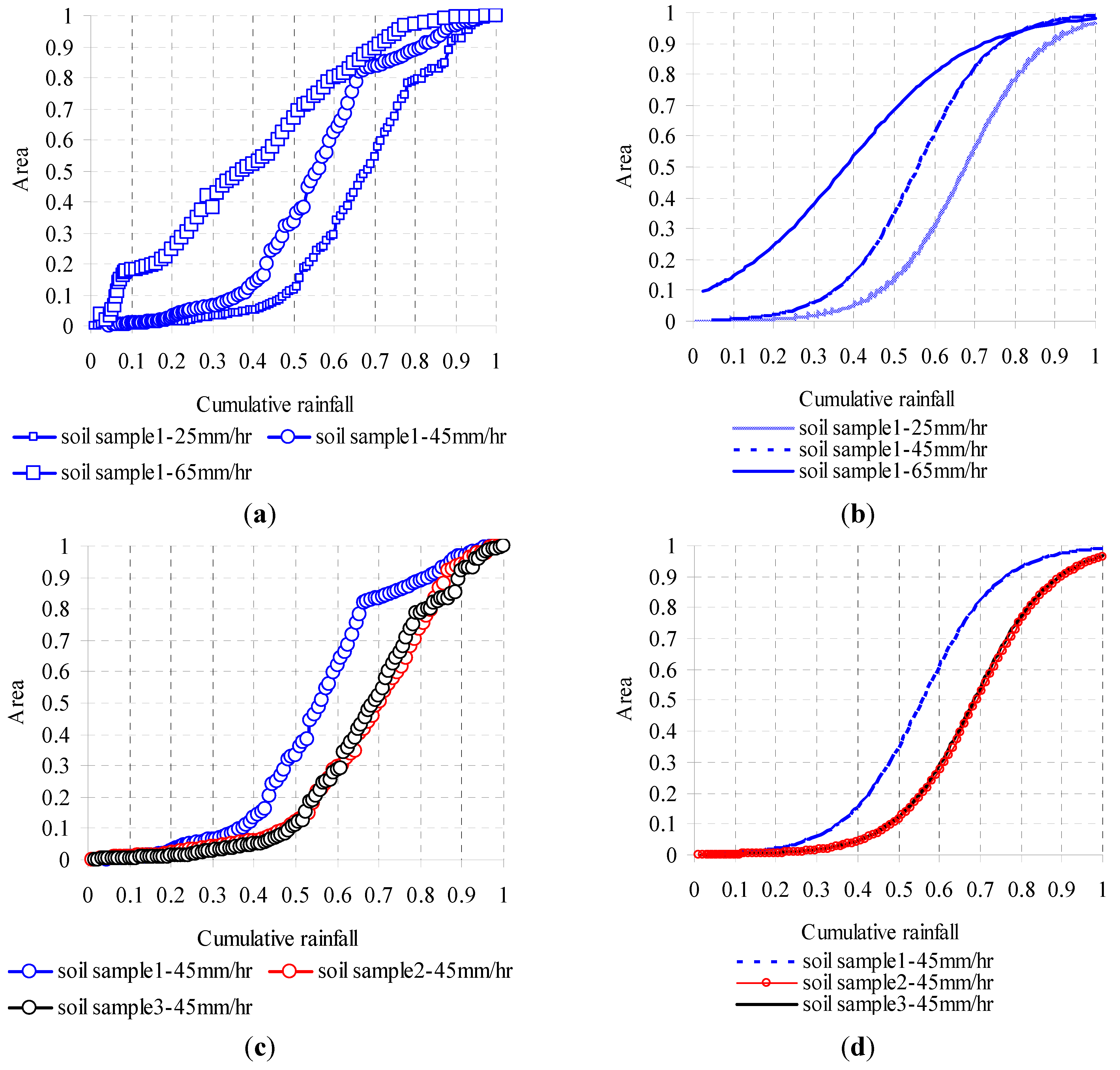
4.1. Dimensionless Quantities of Soil Erosion Area

The developments of the soil erosion area are made as dimensionless plots as shown in Figure 14. For different rainfall intensities, heavy rainfall still has a higher erosion rate; in the second phase, the erosion rate from the light rainfall is greater than that induced by heavy rainfall; in the final stage, all the soil erosion rates have similar trends. In other words, the soil erosion has a first low and then high sensitivity to low rainfall intensity; the soil erosion has a first high and then low sensitivity to high rainfall intensity; in the last stage, they have a similar sensitivity. For different materials, the erosion rate of weak material (Sample 1) is higher than strong material in the first stage; in the second and third phases, there is almost no difference between materials. Thus, it can be considered that the sensitivity of the soil erosion area to material type is not obvious.

Figure 14. Dimensionless plots of soil erosion area: (a) Soil erosion under different rainfall intensity conditions; (b) soil erosion under different rainfall intensity conditions (fitting curve); (c) soil erosion under different material conditions; and (d) soil erosion under different material conditions (fitting curve).

Figure 14. Dimensionless plots of soil erosion area: (a) Soil erosion under different rainfall intensity conditions; (b) soil erosion under different rainfall intensity conditions (fitting curve); (c) soil erosion under different material conditions; and (d) soil erosion under different material conditions (fitting curve).

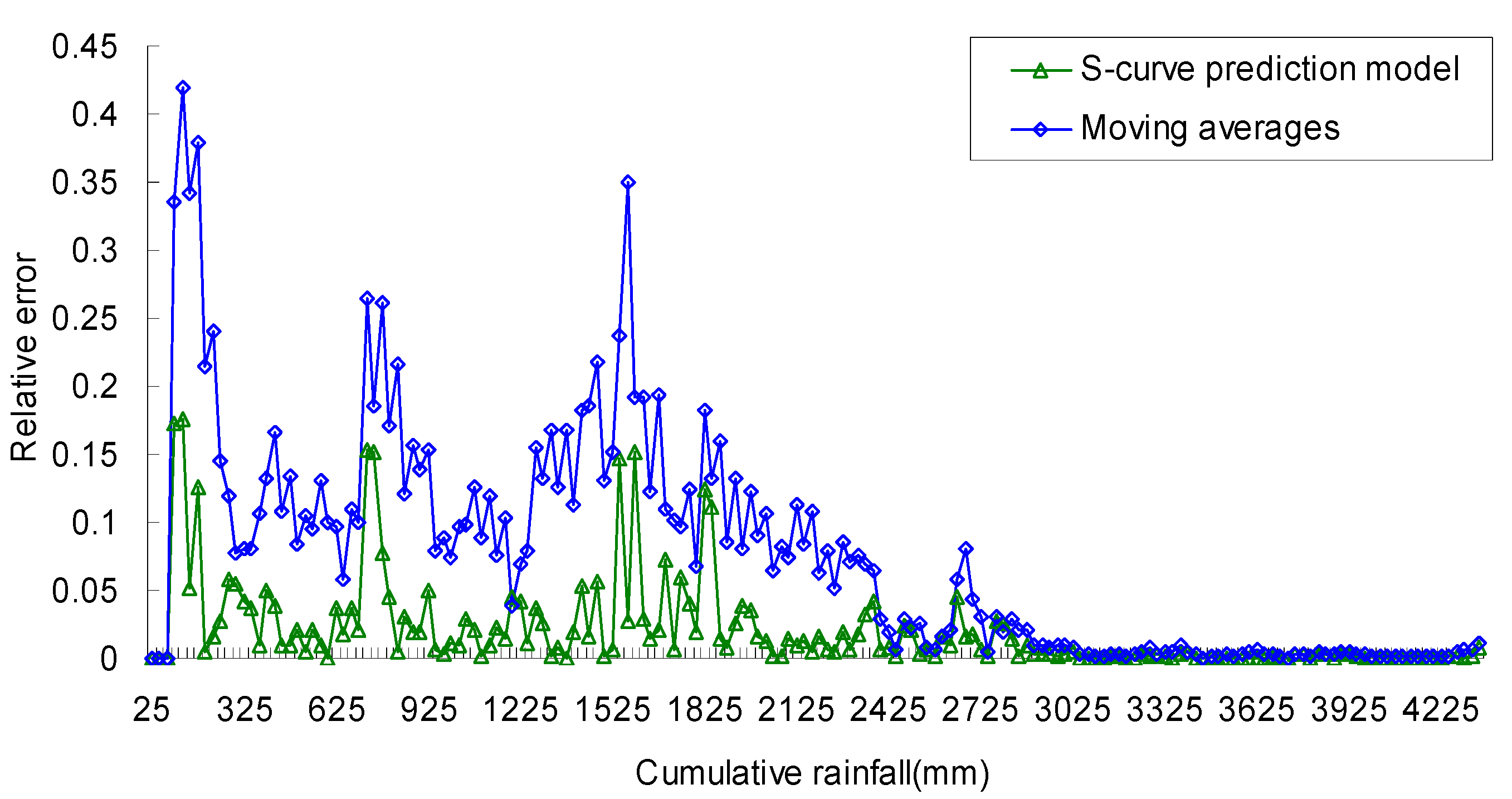
4.2. Comparison Between S-Curve Based Model and Time Series Analysis–Moving Average Model

A case is investigated using a simple time series analysis–moving average method to predict the eroded soil area in Equation (7) [24]. This method in Equation (7) uses the average of the previous three values as the prediction value.

$$s_t\prime =\frac{s_{t-1}+s_{t-2}+s_{t-3}}{3},t\ge 4$$

(7)

where $s_t\prime$ is the output object of the prediction model at time t. $s_{t-1}$, $s_{t-2}$, and $s_{t-3}$ are the observation data at time t−1, t−2, and t−3, respectively. The result is as shown in Figure 15.

Figure 15. Prediction of moving averages method (Sample 1-25 mm/h) (n = 174).

Figure 15. Prediction of moving averages method (Sample 1-25 mm/h) (n = 174).

Firstly, we did relative error analyses for the S-curve prediction model and moving averages model, as shown in Figure 16 (for the case of sample1 under 25 mm/h rainfall). The average relative error of all the experiments is 3%–9.7% for the S-curve prediction model. For the moving averages model, the experimental average relative error is 5.7%–12.1%. The S-curve prediction model includes information on the S-curve trend, and can thus describe the whole process, especially the changes of phase. On the other hand, the moving averages model, whose prediction depends on the previous data, cannot simulate the sudden change of Phase 1 to Phase 2. Thus, in the second stage, error exists all the time until the final stage, reducing the increase of area. It has to be pointed out that the prediction accuracy of the model still depends on the number of predictions. The greater the number of predictions from the model, the lower its accuracy is, while the cost of accurate prediction is a smaller number of forecasts. Secondly, the moving averages model is like a “black box”. Its use only involves giving the input and getting the output without any clear physical meaning and process. In our study, the S-growth curve model framework needs the rainfall intensity and cumulative rainfall (which can be obtained from the rainfall intensity and time) as parameters. It can also describe the three phases of eroded soil area growth from the physical angle. In addition, the model considers different soil materials affecting the erosion area.

Figure 16. Relative error analyses of S-curve prediction model and moving averages model (Sample 1-25 mm/h).

Figure 16. Relative error analyses of S-curve prediction model and moving averages model (Sample 1-25 mm/h).

4.3. Limitation and Suggestion of Experiments

In the current stage, we did not consider the vegetation cover, slope effect and coupled with the rainfall, material effect, because experiments are costly and very time-consuming. Slope shape and surface roughness are relatively simple. As concerns the dimension effect, this is very common for any mini-physical model experiment. In our case, the dimension effect arises mainly from the underestimated rainfall impact and the “boundary effect”. The rainfall bump is reduced by the use of a nozzle spray head in our experiment (we have revised this in Section 2.1). In order to reduce the “boundary effect”, we use a covering of the polytetrafluoroethylene (PTFE), whose friction coefficient is 0.04, on both sides of the flume. In the future, the impact on the soil erosion of the slope effect and coupled the rainfall, slope, and material effect could be our next research direction.

5. Conclusions

In our work, we constructed a physical slope model to investigate to what extent different rainfall intensities and slope materials affect the area of soil erosion acquired by an imaging tool. We further presented an S-curve model to predict the growth of the eroded soil area, which is well trained incrementally and verified efficiently by five physical experiments. The valuable conclusions include:

(1)

The area of soil erosion obeys a trend of an S-growth curve under continuous rainfall.

(2)

A higher rainfall intensity can produce a greater area of soil erosion than lower rainfall intensity for the same material.

(3)

Under the same rainfall intensity, coarse material (stronger material) has a time lag against the soil erosion, but finally a similar area of soil erosion compared to fine material.

(4)

The S-curve model coupled with incremental parameter learning can effectively predict the soil erosion with just the rainfall information as input.

References

1. Wischmeier, W.H.; Smith, D.D. Predicting Rainfall Erosion Losses; USDA Agricultural Handbook, No. 537; U.S. Department of Agriculture: Washington, DC, USA, 1978. [Google Scholar]
2. Renard, K.G.; Foster, G.R.; Weesies, G.A.; McCool, D.K.; Yoder, D.C. Predicting Soil Erosion by Water: A Guide to Conservation Planning with the Revised Universal Soil Loss Equation RUSLE; Agriculture Handbook, No. 703; U.S. Department of Agriculture: Washington, DC, USA, 1997; p. 404. [Google Scholar]
3. Flanagan, D.C.; Nearing, M.A. USDA Water Erosion Prediction Project: Hillslope Profile and Watershed Model Documentation; NSERL report, No. 10; USDA-ARS National Soil Erosion Research Laboratory: West Lafayette, IN, USA, 1995. [Google Scholar]
4. Morgan, R.P.C.; Quinton, J.N.; Smith, R.E.; Govers, G.; Poesen, J.W.A.; Auerswald, K.; Chisci, G.; Torri, D.; Styczen, M.E. The European soil erosion model EUROSEM: A dynamic approach for predicting sediment transport from fields and small catchments. Earth Surf. Process. Landf. 1993, 23, 527–544. [Google Scholar] [CrossRef]
5. Smith, R.E.; Goodrich, D.C.; Quinton, J.N. Dynamic, distributed simulation of watershed erosion: the KINEROS2 and EUROSEM models. J. Soil Water Conserv. 1995, 50, 517–520. [Google Scholar]
6. Soil Erosion: Application of Physically Based Models; Schmidt, J. (Ed.) Springer Science & Business Media: Berlin, Germany, 2013.
7. Nearing, M.A. Capabilities and limitations of erosion models and data. In Proceedings of the 13th International Soil Conservation Organization Conference, Brisbane, Australia, 4–8 July 2004.
8. Pieri, L.; Bittelli, M.; Wu, J.Q.; Dun, S.; Flanagan, D.C.; Pisa, P.R.; Ventura, F.; Salvatorelli, F. Using the Water Erosion Prediction Project (WEPP) model to simulate field observed runoff and erosion in the Apennines mountain range, Italy. J. Hydrol. 2007, 336, 84–97. [Google Scholar] [CrossRef]
9. Cerdà, A. Effects of rock fragment cover on soil infiltration, interrill runoff and erosion. Eur. J. Soil Sci. 2001, 52, 59–68. [Google Scholar] [CrossRef]
10. Ruiz-Sinoga, J.D.; García-Marín, R.; Martínez-Murillo, J.F.; Gabarrón-Galeote, M.A. Precipitation dynamics in southern Spain: trends and cycles. Int. J. Climatol. 2010, 31, 2281–2289. [Google Scholar] [CrossRef]
11. Ruiz-Sinoga, J.D.; Martínez-Murillo, J.F.; Gabarrón-Galeote, M.A.; García-Marín, R. Effects of exposure, scrub position, and soil surface components on the hydrological response in small plots in southern Spain. Ecohydrology 2010, 3, 402–412. [Google Scholar] [CrossRef]
12. Gaskin, G.J.; Miller, J.D. Measurement of soil water content using a simplified impedance measuring technique. J. Agric. Eng. Res. 1996, 63, 153–159. [Google Scholar] [CrossRef]
13. Singh, P.; Kanwar, R.S.; Thompson, M.L. Measurement and characterization of macropores by using AUTOCAD and automatic image analysis. J. Environ. Qual. 1991, 20, 289–294. [Google Scholar] [CrossRef]
14. Romkens, M.J.M.; Prasad, S.N.; Gerits, J.J.P. Soil erosion modes of sealing soils: a phenomenological study. Soil Technol. 1997, 11, 31–41. [Google Scholar] [CrossRef]
15. Le Bissonnais, Y.; Bruand, A.; Jamagne, M. Laboratory experimental study of soil crusting: relation between aggregate breakdown mechanisms and crust structure. Catena 1989, 16, 377–392. [Google Scholar] [CrossRef]
16. Andrea, R.; Helming, K.; Diestel, H. Effect of antecedent soil water content and rainfall regime on microrelief changes. Soil Technol. 1997, 10, 69–81. [Google Scholar]
17. Backus, D.; Kehoe, P.J.; Kydland, F.E. Dynamics of the Trade Balance and the Terms of Trade: The S-curve; National Bureau of Economic Research: Cambridge, MA, USA, 1992. [Google Scholar]
18. Bejan, A.; Lorente, S. The constructal law origin of the logistics S curve. J. Appl. Phys. 2011, 110, 024901. [Google Scholar] [CrossRef]
19. Sun, W.; Won, S.H.; Ju, Y. In situ plasma activated low temperature chemistry and the S-curve transition in DME/oxygen/helium mixture. Combust. Flame 2014, 161, 2054–2063. [Google Scholar] [CrossRef]
20. De Massis, A.; Chirico, F.; Kotlar, J.; Naldi, L. The temporal evolution of proactiveness in family firms: The horizontal S-curve hypothesis. Fam. Bus. Rev. 2013. [Google Scholar] [CrossRef] [Green Version]
21. Van Rompaey, A.; Krasa, J.; Dostal, T.; Govers, G. Modelling sediment supply to rivers and reservoirs in Eastern Europe during and after collectivisation period. Hydrobiologia 2003, 494, 169–176. [Google Scholar] [CrossRef]
22. USDA–Water Environment Prediction Project: Hillslope Profile and Watershed Model Documentation; Flanagan, D.C.; Nearing, M.A. (Eds.) US Department of Agriculture–Agricultural Research Service, National Soil Erosion Research Laboratory: West Lafayette, IN, USA, 1995.
23. Bathurst, J.C.; Wicks, J.M.; O’Connell, P.E. The SHE/SHESED basin scale water flow and sediment transport modelling system. In Computer Models of Watershed Hydrology; Singh, V.P., Ed.; Water Resource Publication: Highlands Ranch, CO, USA, 1995; pp. 563–594. [Google Scholar]
24. Hamilton, J.D. Time Series Analysis; Princeton University Press: Princeton, NJ, USA, 1994; Volume 2. [Google Scholar]