Undersampling in Orthogonal Frequency Division Multiplexing Telecommunication Systems

Computer Engineering Department, Technological Educational Institute of Thessaly, Larissa, 41110, Greece
Appl. Sci. 2014, 4(1), 79-98; https://doi.org/10.3390/app4010079
Submission received: 12 September 2013
/
Revised: 24 February 2014
/
Accepted: 28 February 2014
/
Published: 17 March 2014
(This article belongs to the Special Issue Digital Signal Processing and Engineering Applications)
Abstract
:Several techniques have been proposed that attempt to reconstruct a sparse signal from fewer samples than the ones required by the Nyquist theorem. In this paper, an undersampling technique is presented that allows the reconstruction of the sparse information that is transmitted through Orthogonal Frequency Division Multiplexing (OFDM) modulation. The properties of the Discrete Fourier Transform (DFT) that is employed by the OFDM modulation, allow the estimation of several samples from others that have already been obtained on the side of the receiver, provided that special relations are valid between the original data values. The inherent sparseness of the original data, as well as the Forward Error Correction (FEC) techniques employed, can assist the information recovery from fewer samples. It will be shown that up to 1/4 of the samples can be omitted from the sampling process and substituted by others on the side of the receiver for the successful reconstruction of the original data. In this way, the size of the buffer memory used for sample storage, as well as the storage requirements of the Fast Fourier Transform (FFT) implementation at the receiver, may be reduced by up to 25%. The power consumption of the Analog Digital Converter on the side of the receiver is also reduced when a lower sampling rate is used.
1. Introduction
Sampling a signal at a frequency below the Nyquist rate is often called undersampling and is used when information that is changing at a relatively low rate is transmitted over a high frequency carrier. In these cases, the sampling on the side of the receiver is performed at a rate that is twice the information bandwidth instead of the peak frequency. A common practice is to sample an Intermediate Frequency (IF) rather than the baseband one [1]. Two popular techniques for the reconstruction of a signal from fewer samples than the ones required by the Nyquist rate, are the Compressed Sensing and the Kalman filters.
Kalman filters [2,3,4,5] are used in a variety of applications ranging from economics to vehicle navigation, especially for tracking the value of dynamic parameters in noisy environments. They can also be used for the reconstruction of a signal with fewer samples in real time by applying a two step recursive process: (a) prediction, where the current state variables are estimated, and (b) update of the estimated values, when the next measurement is available. Real time signal reconstruction approaches based on Very Large Scale Integration (VLSI) implementations have been proposed in the past, based on Kalman filters [6]. A VLSI implementation of a Kalman filter, where multiple parallel operations can be performed in a single iteration, is described in [7].
The Compressed (or Compressive) Sensing or Compressed Sampling techniques are also based on undersampling of sparse, or in more general terms, compressible information. One of the first approaches in this field has been published in [8]. A Compressed Sensing (CS) technique that is more appropriate for hardware implementation has been proposed in [9] for general applications. In these Compressed Sensing approaches, the original information recovery is performed by only a small number of samples, much smaller the number required by the Nyquist rate. By the term sparse it is meant that most of the original data values must have a trivial common value like zero (or near zero). If the original data values are compressible, although they may not be sparse, they can be expressed with fewer values, e.g., a piece of line in an image can be defined only by two points and there is no need to store the coordinates of all the intermediate points. Sometimes, the differences between successive samples are zero instead of the absolute values and these sparse differences are taken into consideration in order to apply CS techniques. Formally, an M × N matrix is considered to be S-sparse if only S of its values are non-zero with S << M × N. In this paper, the sparse information will also be expressed as the fraction of non-trivial values, e.g., in a signal with 1% sparseness, only 1% of its values are non-zero.
A CS problem can be simply modeled as:
y = Ax + e
The vector x (size: Nd) in Equation 1 is the original input, y is the actual measurement (size: M << Nd), and e is an M-size vector representing noise or the error from the input recovery. The matrix A (size: MxNd) can represent the digitization process. As Equation 1 does not have a single solution, the adopted CS method tries to find a vector x that fits Equation 1 with an acceptable approximation error e. The following optimization target has been proposed in various CS approaches in order to locate such an appropriate solution for vector x:
![Applsci 04 00079 i015]()
The Lp norm (p = 2 in most implementations) is used to restrict the difference between y and Ax below the threshold th. The matrix A can be expressed as a product of other matrices with special features (e.g., partial Fourier or Hamadad matrices) and the minimization (2) can be applied to the product of x with one of these elementary matrices.
Iterative and/or greedy algorithms have been proposed in order to solve the optimization problem defined above like: basis pursuit, gradient project, gradient pursuit, non-convex projection, Iteratively Reweighted Least Squares (IRLS), Orthogonal Matching Pursuit (OMP), Compressive Sampling Matching Pursuit (CoSaMP), Subspace Pursuit (SP), Iterative Hard Thresholding (IHT), etc. However, all of these iterative or recursive algorithms require hardware implementations of high complexity and thus the gain by the use of a lower cost/speed/power Analog Digital Converters (ADC) is often cancelled. Surveillance applications can take advantage of CS techniques as described in [10]. Sensor networks can also benefit from CS algorithms [11]. The authors of [12] describe a higher level CS approach incorporated in a wireless multimedia sensor network in which the images from multiple cameras are used. In [12], the differences between successive frames are used in order to get a CS modeling where only a few pixels are non-zero.
The CS and the Kalman filter signal reconstruction approaches that were referenced above, are iteratively solved, e.g., by greedy algorithms. Kalman filters are more appropriate for hardware implementations with reusable resources although the iterative procedure required to update the state variables takes time that may be critical for real time applications. This can be solved with pipeline architectures but additional hardware resources will be required.
The CS approaches have not been used for the reconstruction of the original data in Orthogonal Frequency Division Multiplexing (OFDM) environments because even if they are sparse, the encoding, the interleaving and the IDFT applied at the transmitter, cancel their sparseness. However, several CS techniques have been applied in order to reduce the number of pilot symbols required for channel estimation and thus exploit more efficiently the available bandwidth [13,14,15].
An undersampling approach that is not based on difficult optimization problems is presented in this paper, which can be implemented in real time environments with low cost/complexity hardware. The prerequisite is to have a high degree of sparseness in the original information. If this condition is true, the properties of the Fourier transform can be exploited in order to estimate the values of several samples by others that have already been retrieved. There are also some restrictions that have to be obeyed concerning the employed Interleaving and Forward Error Correction (FEC) methods. The complexity of the Discrete Fourier Transform (DFT) implementation can also be reduced using the proposed method if for example a Digital Signal Processor (DSP) or Column recursive radix-2 Fast Fourier Transform (FFT) implementation is employed.
The number of samples required by the proposed technique, for the original information recovery, is higher compared to the number of samples required by a CS approach. However, it can be implemented with very low cost and high speed hardware since it is based on a non-iterative procedure with fixed steps. The proposed method includes: (a) an appropriate bit and/or channel interleaving/deinterleaving procedure, (b) the use of a FEC encoding scheme with a minimum data rate of 1/2, (c) Analog Digital Converter (ADC) sampling control at the side of the receiver and (d) the estimation of samples that have not been retrieved by the ADC from other available samples by simply copying their value. The aforementioned four steps are incorporated in the modeling of an OFDM system in MATLAB. The results from the simulation of this model show that in many cases, the Bit Error Rate (BER) is zero or at least very low (below 10−4) using the proposed method.
The architecture of an OFDM system is presented in Section 2. The proposed undersampling method and the architecture of the corresponding OFDM transceiver are described in Section 3. The effect of the proposed method to the FFT implementation is discussed in Section 4. Finally, simulation results are presented in Section 5.
2. The Architecture of an OFDM System
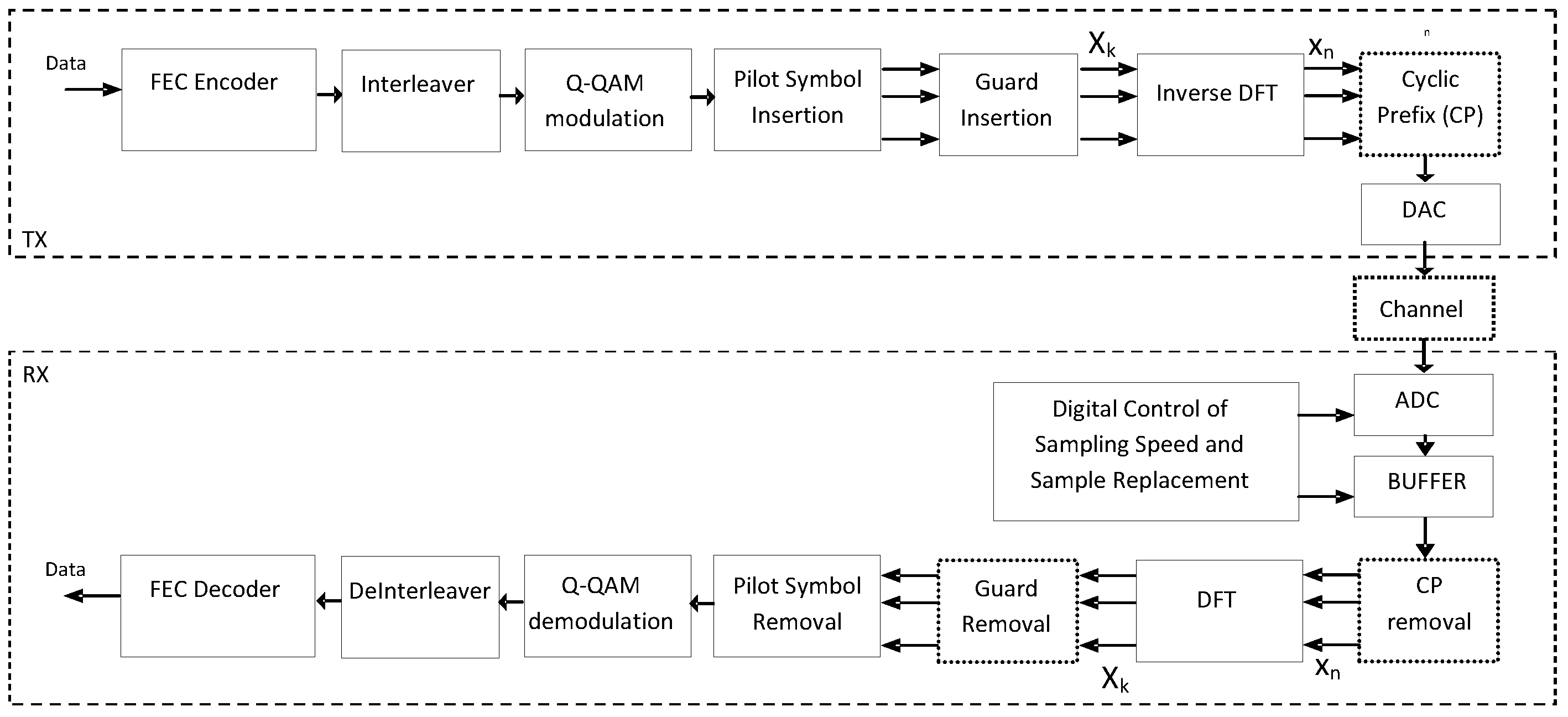
The OFDM modulation is used in several telecommunication standards. The architecture of an environment that is based on OFDM modulation is shown in Figure 1. The input data are encoded at the transmitter and along with the generated parity bits are interleaved and modulated using Q-Quadrature Amplitude Modulation (Q-QAM). “Pilot” symbols are inserted assisting the receiver in the estimation of the channel condition (e.g., multipaths, fading, etc.). This sequence of Q-QAM symbols Xk (data, parity, pilots) may be padded with an appropriate value forming an input set of values for the Inverse Discrete Fourier Transform (IDFT) that generates the time symbols xn. Both xn and Xk symbols are complex numbers. The time symbols xn and are transmitted over the channel either in baseband mode or by mixing them with a high frequency carrier. Cyclic Prefix (CP) is added to avoid Inter-Symbol Interference (ISI) and Inter-Carrier Interference (ICI). A Digital to Analog Converter (DAC) at the transmitter converts the arithmetic values of the IDFT output and the CP symbols into the analog signal that will be transmitted over the communication channel. A pair of DACs may be used to convert separately the real and imaginary parts of these symbols. Although this analog signal may be transmitted over a high frequency carrier as stated earlier, the details of this case will not be discussed since they do not affect the proposed undersampling method. The channel adds Additive White Gaussian Noise (AWGN). Channel fading, multipaths, etc., are additional noise sources that should be taken into consideration for more accurate modeling of OFDM channels but for simplicity reasons the proposed undersampling technique will be evaluated using only a broad range of AWGN noise at the channel. The receiver can sample the distorted by the channel noise xn real and imaginary parts by a pair of ADCs after ignoring the CP part. The symbols Xk are recovered at the output of a DFT. The padding symbols and the pilots are removed and the remaining Q-QAM data and parity symbols are mapped-back to data/parity bits, deinterleaved and feed the input of the FEC decoder. The Cyclic Prefix, CP Removal, and Guard Removal blocks are placed in dotted boxes to indicate that they will not play an important role in the simulations that will be described in Section 5.
Figure 1.
Architecture of an OFDM system.

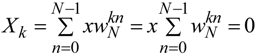
The OFDM modulation is an improvement of Frequency Division Multiplexing (FDM) and can be viewed as a transmission of the N, Xk symbols over N different subcarriers. Although these subcarriers have a small frequency difference, they are orthogonal to each other and, thus, their interference is minimal. The DFT and the Inverse DFT (IDFT) transforms are defined by the Equations 3 and 4 respectively:
![Applsci 04 00079 i001]()
![Applsci 04 00079 i002]()
where the ![Applsci 04 00079 i003]() and
and ![Applsci 04 00079 i004]() are the twiddle factors and j2 = −1.
are the twiddle factors and j2 = −1.
 and
and  are the twiddle factors and j2 = −1.
Figure 2.
Distribution of the parameters Xk to different twiddle angles for the estimation of the xn values in a 16-point DFT.
Figure 2.
Distribution of the parameters Xk to different twiddle angles for the estimation of the xn values in a 16-point DFT.
3. The Proposed Undersampling Method
The DFT transform has some interesting properties that can be exploited if the input data are sparse. Consider for example the matrix representation of a 16-point DFT displayed in Figure 2 that visualizes the concept on which the proposed method is based. As can be seen from this figure, there are pairs of rows that have a different number of identical Xk positions than others. For example, the row for n = 0 differs from the row that corresponds to n = 8 at the position of 8 Xk values while, the rows for n = 1 and n = 15 have only two common Xk positions (k = 0 and k = 8). The equation x1 = x15 would hold if for the real part of the twiddles we had:
![Applsci 04 00079 i005]()
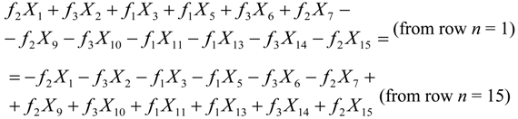
Where f1 = 0.382683, f2 = 0.92388, f3 = 0.707107 (the cosine or sine of the various twiddle angles). In a similar manner for the imaginary part of the twiddles we would get:
![Applsci 04 00079 i006]()
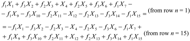
Combining Equations 5 and 6 in order to have x1 = x15 we get the following conditions that must to be true:
![Applsci 04 00079 i007]()
![Applsci 04 00079 i008]()
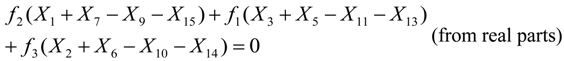

There are several relations between the Xk symbols for the Equations 7 and 8 to hold. For example, if all the Xk symbols are zero or if the Xk symbols in each one of the parentheses sum up to zero as follows:
X1 + X7 = X9 + X15
X3 + X5 = X11 + X13
X2 + X6 = X10 + X14
X3 + X5 = X11 + X13
X2 + X6 = X10 + X14
If the condition of Equation 9 holds, then the symbol x15 can be used in the place of x1 or vice versa. Conditions like the ones of Equations 5–9 can be found for other pairs of xn symbols but the target is to find the smallest number of conditions that hold for a large number of xn symbol pairs. This is not a trivial task since each conditions depends on the selected xn symbol pair, the size of the DFT and the exact values that the symbols Xk can have, which in turn depends on the employed Q-QAM modulation.
Substitutions like the one of x1 by x15 described above and the applications where conditions, such as Equations 5–9, can occur will be studied in our future work. A more general condition can be found though, since the xn symbols with odd n (n = 2p + 1, p = 0, 1, 2,…, N − 1) are equal to the symbols x2p + 1 + N/2, with N = 4F if X2t + 1 = X2t + 1 + N/2 for t between 0 and F−1. Using Equation 4 this can be proven as follows:
![Applsci 04 00079 i009]()
![Applsci 04 00079 i010]()
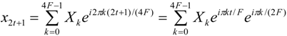
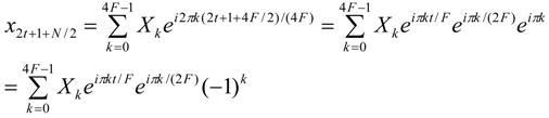
From Equations 10 and 11 it is obvious that the twiddle factors at even k positions are equal since (−1)k = 1 if k is even. At odd k positions the twiddle factors are inverted and x2t + 1 = x2t + 1 + N/2 only if Xk = 0. Unfortunately, Xk is never equal to zero if it is a Q-QAM output symbol. However, if the symbols Xk and Xk + N/2 (=Xk + 2F) are equal, the following equation is true:
![Applsci 04 00079 i011]()
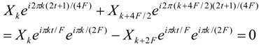
Equation 12 focuses on two terms of the sum in Equation 15 and means that the pairs Xk and Xk + 2F multiplied by the corresponding twiddle factors cancel each other in Equation 10 if they are equal. The same holds for Equation 11. If X2t + 1 = X2t + 1 + N/2 holds for almost all t < F, then all the Xk symbols with odd k add up to a zero or near zero value and this can be achieved if these symbols are derived by sparse data. In this case, half of the xn symbols at the odd positions can replace the rest of the xn symbols with odd n. Thus, the receiver can avoid sampling (or storing) up to F values since they can be estimated by other already available values. The number of the samples that can be substituted by others can be further increased if additional restrictions apply to the relation between the Xk values as was shown by the Equations 5–9.
In order to have Xk symbols with identical value placed at odd k-positions, an appropriate interleaving and FEC encoding should be employed. Even in this case, a few Xk symbols will not be equal to the common value (denoted Xcv henceforth) of the rest of the Xk symbols, since the input data are sparse but not all zero. A perfect reconstruction of the input data is not always feasible due to this fact but the employed FEC method helps in achieving a low enough bit error rate.
The data rate R of the employed FEC encoder, should be greater or equal to 1/2. This is because if R = 1/2, the data and the parity bits can be grouped separately by the Q-QAM modulator of Figure 1. In this case, half of the Xk Q-QAM symbols will correspond to data and most of them will have the same trivial value Xcv due to the sparseness of the original data. These Xcv symbols should be placed by the interleaver at the odd positions. If R > 1/2, the proposed method is still applicable as there will be additional data Xk symbols (most of them will be equal to Xcv) that will be placed at even positions. However, R < 1/2 is not recommended because some parity symbols will have to be placed at odd positions increasing the number of the symbols with different value than Xcv and, thus, the efficiency of the proposed method will be reduced. The transmission capacity is not confined since the proposed method is not suggested only for cases where the data rate R is low. On the contrary it is preferably applied when R ≥ 2, i.e., when most of the transmitted bits are data and not parity.
The interleaving method followed is not common to all standards and configurable interleavers are proposed to meet different requirements. An optimal interleaving strategy depends on many factors like, the data rate R, the decoding algorithm used, its randomness, the minimum distance where a value should be moved, etc. In [16] an appropriate interleaving scheme is proposed for Turbo Code decoders that use the min-sum algorithm. In the simulation results of this work it is shown that the higher the data rate R is, the higher is the BER. Moreover, a difference in the BER in the order of 10−3 can be observed between different interleaving schemes for the same SNR. The interleaver in the method proposed in this paper is allowed to do any permutation separately in the data and the parity bit stream. It is also allowed to permute in a random way the data Q-QAM symbols between odd positions and the parity Q-QAM symbols between even positions but it is not allowed to move data symbols to even positions and parity symbols to odd positions. The interleaving scheme followed in this paper includes a pseudo random permutation in the log2Q bits of each Q-QAM symbol.
Figure 3.
Order of (a) padding symbols, (b) parity and data symbols after a pilot at even position, and (c) parity and data symbols after a pilot at odd position.
Figure 3.
Order of (a) padding symbols, (b) parity and data symbols after a pilot at even position, and (c) parity and data symbols after a pilot at odd position.
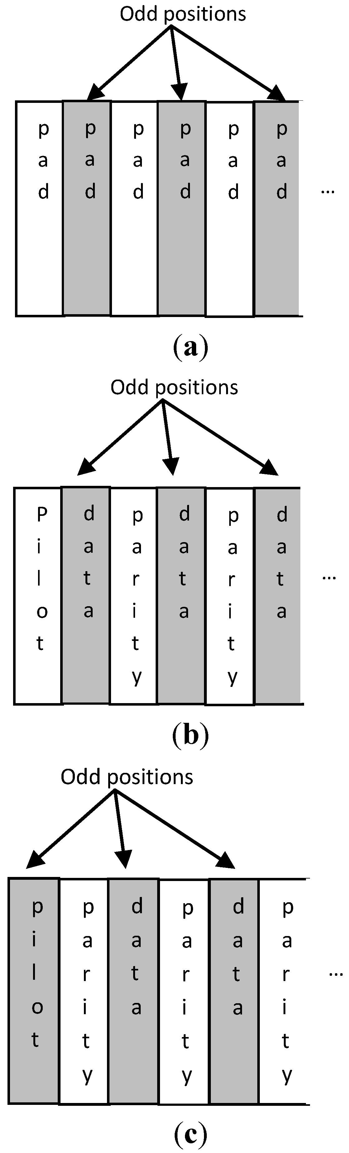
The encoding and interleaving scheme followed in this work has also to take into account the fact that pilot and padding symbols will be added before the IDFT transform. These pilot and padding symbols do not affect the proposed undersampling method if they are defined equal to the Xcv value.
In the following, a Recursive Convolutional Systematic (RSC) encoder is used with a systematic and a parity output of data rate R = 1/2. The original data bits are available at the systematic output while the parity bits are generated by the feedforward path described by the polynomial 1 + D + D2 + D3 and the feedback path that is described by 1 + D + D2. A small 8-bit buffer at the output of the encoder groups the 4 data and 4 parity bits into a pair of 16-QAM symbols.
The 16-QAM data symbols can be reordered by a channel interleaver and then placed at odd positions. Similarly, the 16-QAM parity symbols can be potentially reordered and placed at even positions. Such channel interleavers will be tested in the framework of different Q-QAM modulations in our future work. The bit and channel interleavers described above can have a fixed routing from their inputs to their outputs for lower complexity. The order of the intermediate data and parity symbols may be reversed if necessary since a number of padding and pilot symbols have to be inserted as shown in Figure 3. In Figure 3a, it is shown that Xcv values will anyway be placed at the odd positions in the region of the padding symbols, since the padding value is selected to be Xcv. At a region that starts with a pilot at even position, the order of the following Q-QAM symbols must follow the recurring pattern <data, parity> (see Figure 3b). The proposed undersampling method is not affected if a pilot is placed at an odd position provided that its value is chosen to be Xcv. The following symbols have to the recurring pattern: <parity, data> (see Figure 3c). In this way the same Xcv value will be placed in the majority of the odd positions at the set of points that will serve as input to the IDFT. The interleaving policy described above can be implemented with trivial hardware without increasing the system complexity.
At the side of the receiver, the sampling of the F, x2t + 1 symbols by the ADC may be omitted as they can be substituted by the F symbols: x2t + 1 + N/2 or vice versa. The original and the substituted xn values form the input of the DFT. A low complexity finite state machine implemented in hardware can control the sampling rate of the ADC preventing the sampling of the values that can be substituted by others. In this way, 50% of the time interval that is needed to receive the N, xn symbols, the ADC operates at half of its normal sampling rate lowering its power consumption. If a smaller number of xn values are substituted by others the lower ADC sampling rate will be applied in a shorter time interval. For example, if only half of the x2t + 1 + N/2 symbols are substituted (e.g., the x2t + 1 + N/2 + N/4) in order to achieve a better BER, the lower ADC sampling rate will be applied to the 25% of the time interval that is needed to receive all the xn symbols required for a N-point DFT. The power consumption of the ADC may be reduced to the half during these intervals as it is proportional to the sampling frequency. In addition to the ADC power consumption reduction, the buffering memory where the ADC samples are stored can be smaller (by up to F locations) and the FFT implementation of the DFT can be simpler as will be discussed in the next section.
A full advantage of the reduced ADC power, the buffering memory and the simpler FFT implementation can be taken if only sparse data are exchanged, i.e., if the developed OFDM transceiver is dedicated to applications that exchange exclusively data like MRI or radar images, sensor values, etc. If the sparse data are transmitted occasionally, then specific parts of the OFDM receiver (like a butterfly of the FFT) can be deactivated after the detection of sparse data. The detection can be based on the output of the receiver (after the FEC decoder) by measuring the non-zero bits. If the fraction of the non-zero bits compared to the total number of data bits is smaller than a threshold, e.g., 2%, then the lower ADC sampling rate, the sample substitution and the reduced buffering are activated for as long as the observed data are sparse.
4. FFT Implementation Issues
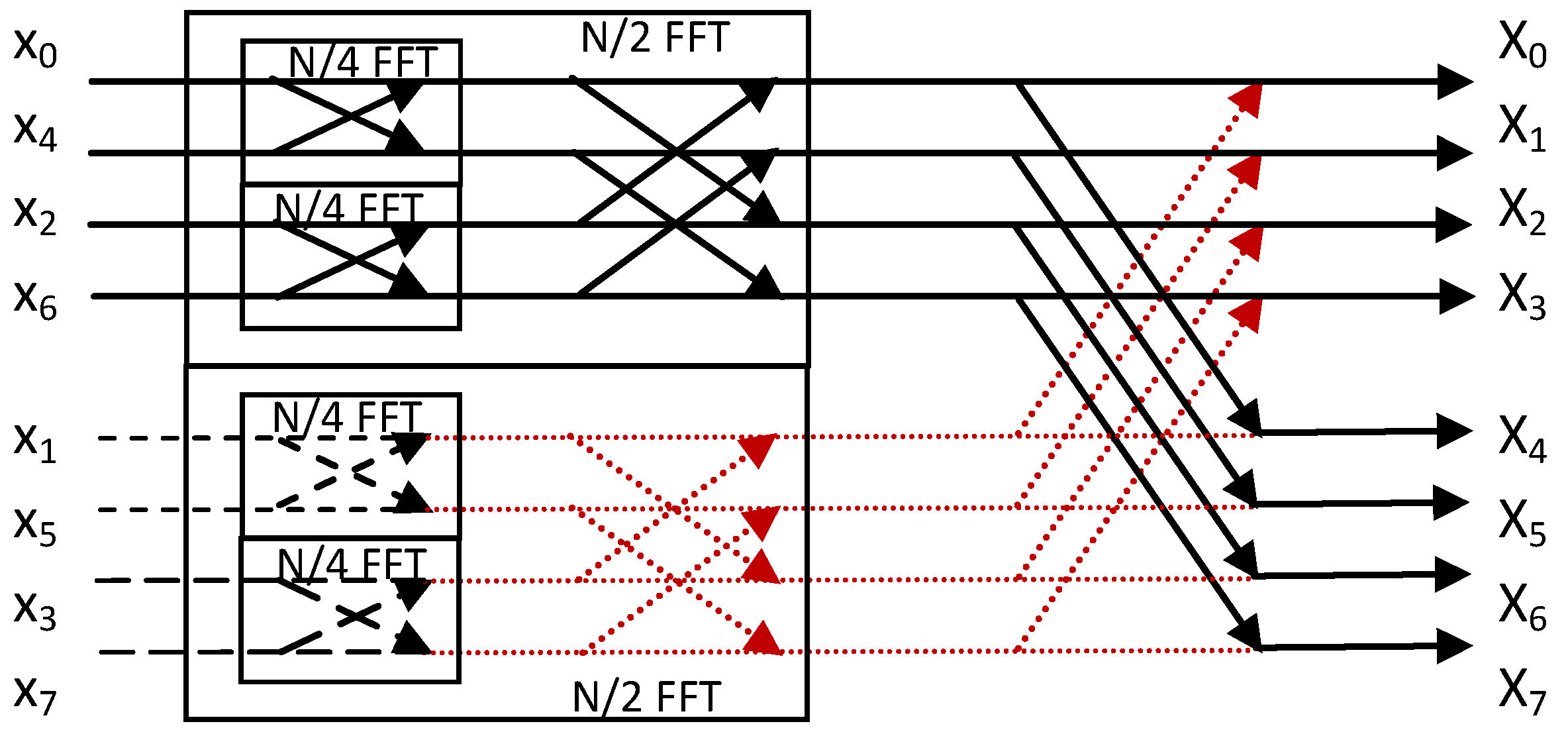
The DFT required in OFDM environments is implemented efficiently using Decimation In Time (DIT) FFT as was proposed in the mid-sixties by Cooley and Turkey [17]. Instead of performing all the calculations dictated by Equation 3 the DFT can be estimated from two or more elementary DFTs avoiding the calculation of the same parameters multiple times. For example, in a radix-2 FFT an N-point FFT is performed by combining a pair of N/2 point FFTs. One of these FFTs accepts as input the odd inputs of the N-point FFT and the other one the even inputs. Each one of these N/2 point FFTs is also implemented by a pair of N/4-point FFTs and so forth until 2 point FFTs are defined. In this way the N2 operations required by the initial N-point FFT are reduced to Nlog2N. This architecture is shown for the case of an 8-point radix-2 FFT in Figure 4 [18]. The inputs are bit reversed while the outputs are in normal order.
Figure 4.
Implementation of an 8-point DFT as a radix-2 DIT FFT (the red arrows indicate zero butterfly outputs).
Figure 4.
Implementation of an 8-point DFT as a radix-2 DIT FFT (the red arrows indicate zero butterfly outputs).

The N/4 point FFT which for the case of Figure 4 is actually a 2-point FFT defines the butterfly operation between its two inputs xi0 and xi1:
![Applsci 04 00079 i012]()
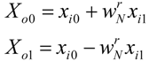
The twiddle factors w, multiply the input symbol xn that corresponds to the diagonal arrow in a butterfly and their product is added to the complex symbol value assigned to the horizontal line that meets the end of the diagonal arrow. For simplicity reasons, the twiddle factors were not displayed in Figure 4.
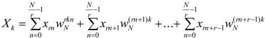
Each of the terms in Equation 14 represents one of the r elementary N/r point FFTs that are combined to implement an r-radix FFT. The overall arithmetic operations required by an N-point FFT decrease when r is high but the complexity of each butterfly increases since (a) a higher number of complex arithmetic operations is required, (b) the number of butterfly inputs is high, (c) the connectivity is more complicated, and (d) the critical path delay in the butterfly is also high. High radix FFTs are not very popular as their VLSI implementation is more difficult. Their advantage though, is that the number of multiplications and the number of stages (corresponding to global communication and memory accesses to execute FFTs) decreases [20].
Although, some alternatives of the proposed undersampling technique may cooperate more efficiently with high-radix FFTs we will focus on the affect of the proposed scheme to the implementation of a radix-2 FFT like the one shown in Figure 4.
The xn pairs in the 2-point FFTs that are grouped in the N/2-point FFT with the odd positioned values are the pairs: x2p + 1 and x2p + 1 + N/2 that are expected to be equal (denoted by the same type of dashed lines in Figure 4) as described in the previous section. The result of a DFT with equal xn symbols (xn = xc) is zero (the dotted red lines in Figure 4):
![Applsci 04 00079 i014]()
As can be shown from Figure 4, all the N-point FFT outputs in this case are determined by only the outputs of the N/2-point FFT with the odd positioned input symbols. These, will be half of the outputs of the N-point FFT while the rest will be determined by the same N/2-point FFT outputs multiplied by the appropriate twiddle factor. In other words, the N/2-point FFT with the odd positioned input symbols can be completely removed. However, as we will see in the next section, if 25% of the xn symbols at the receiver are substituted by the value of other available samples, a non-negligible error floor is posed. The error floor is much lower if 12.5% of the xn symbols at the receiver are substituted, i.e., a quarter of the odd positioned xn symbols. In this case, an N/4-point FFT can be removed reducing the die area needed for its VLSI implementation. Of course, if the exchanged information is not sparse all the time, the N/4-point FFT must not be removed but can be deactivated for lower power consumption when sparse information reception is detected.
The FFT requires Random Access Memory (RAM) memory for storing both its input and its intermediate results. The twiddle factor coefficients are usually stored in Read Only Memory (ROM). In VLSI FFT implementations with single memory, the butterflies are using the same memory for storing their inputs and their results requiring lower memory but they are slower since reading the input and writing the output values cannot be carried out concurrently. In dual memory architectures the butterfly results are stored in a separate memory concurrently with the reading of the input values. Pipeline architectures consist of multiple stages with intermediate storage requirements, thus, they have the highest memory requirements but they also can achieve the highest speed.
Several more advanced FFT implementations have been proposed, with low memory requirements without compromising speed. In [21], a single radix-4 FFT with partitioned memory is used to implement a 256-point FFT in 6 us complying with the HomePlug standard. The required total RAM memory size is N in this architecture. In [22], a pipeline butterfly module is described requiring N RAM words grouped in two banks. In [23], the FFT implementation for an 8 × 8 Multiple Input Multiple Output (MIMO) OFDM system is described. The 128-point Mixed Radix Multi-path Delay Commutator (MRDC) described in [23] accepts as input the eight streams of the MIMO system. The role of the input and output RAMs is data arrangement between the adjoined OFDM blocks such as OFDM subcarrier assignment and guard interval insertion. It is obvious from the FFT implementations in [21], [22] and [23] that not all of the inputs of the FFT are stored in RAM. In fact in most of the implementations only half of the input values need to be stored initially and the rest are driven directly to the FFT inputs. Consequently, if an FFT implementation requires N RAM words, half of the words are used for input storage and the rest of them are used for intermediate results. In fact, in implementations like [22], even the N/2 words that are initially used for input values’ storage, are also later used for storing intermediate results.
Figure 5.
Original FFT implementation of [22] (a) and Modified FFT implementation for the proposed undersampling method (b). The operations with the red font in Figure 5b indicate trivial operations that can be omitted.
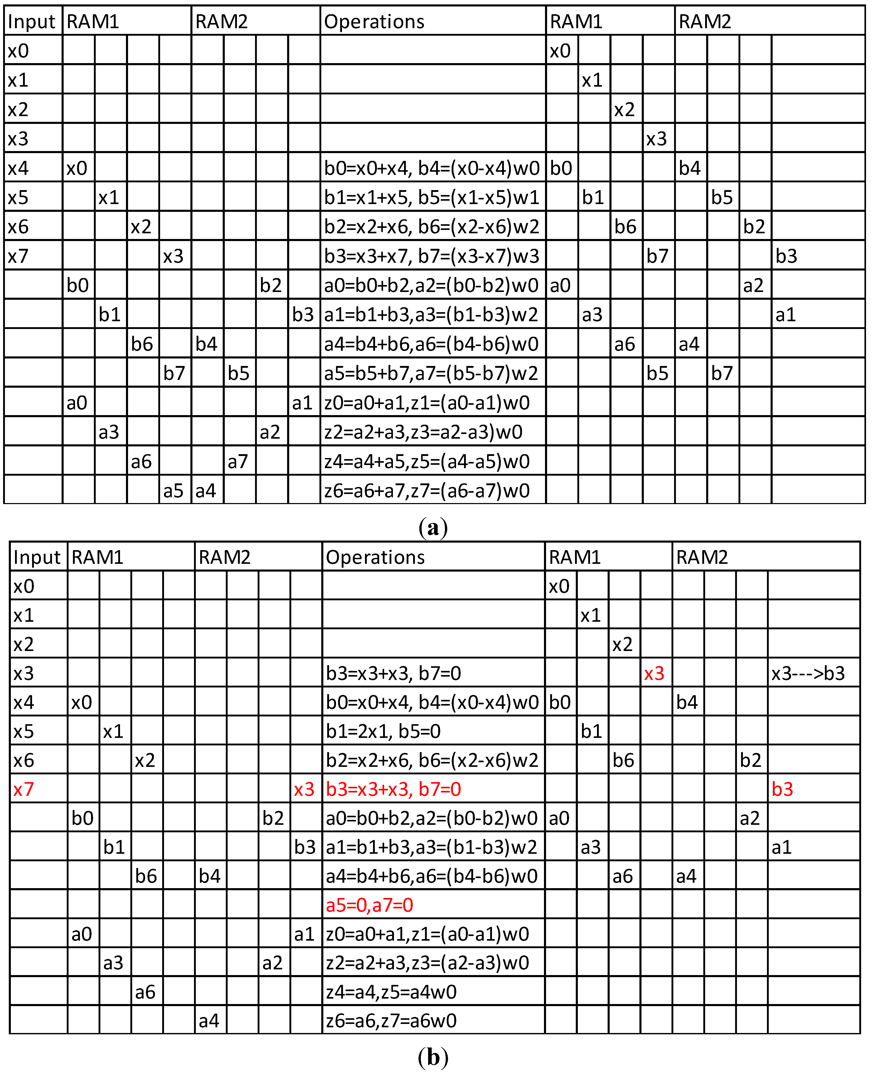
In this paper, we assumed that in the general case all the input values are stored initially in a RAM buffer and the 25% reduction that can be achieved is referring to this buffer as is the case in [23]. However, if sparse input data are used, then the trivial values appearing at the outputs of some FFT blocks, also affects the storage requirements for intermediate results. Thus, we can state that the 25% reduction in the memory requirements achieved by the proposed undersampling method, applies to the whole FFT architecture. This fact can be demonstrated by the 8-point example FFT architecture described in [22]. By slightly modifying the multiplexing scheme of the Memory Based FFT (MBFFT) presented in [22], the operations needed and the memory required for this 8-point FFT is shown in Figure 5.
In Figure 5a, the original operations described in [22] are presented for an 8-bit FFT. Each one of the two RAM banks (RAM1 and RAM2) has four words and the RAM contents at the left are the input values to the operations shown in the middle column. The RAM contents at the right are the output values of these operations. The parameters a and b are intermediate results (butterfly outputs) while w are the twiddle factors stored in a separate ROM and z are the results. As described in our approach, x5 and x7 are expected to be equal to x1 and x3, respectively. Using this fact, the simplified table of Figure 5b can be generated from Figure 5a. As can be seen in Figure 5b, each one of the RAM banks has an unused column now, showing that the memory requirements have been reduced by 2/8 or 25%. Moreover, the two red rows in Figure 5b show that the operations needed there have already been carried out earlier and the FFT procedure is now two steps shorter. Finally, only the coefficients w0 and w2 are used in Figure 5b, thus the ROM words have also been reduced by 50%.
5. Simulation Results
In this section, the simulation results from the encoding, the interleaving and the sample substitute policy described in the previous sections will be presented for a diversity of data sparseness degrees and substituted samples. The system has been described in MATLAB and includes all the OFDM stages that have been described by Figure 1. The input to the FEC encoder at the transmitter is a data packet of 1536 bits and the RSC encoder described in Section 3 that is used as the FEC encoder of Figure 1 generates 1536 parity bits mapped to 384 data and 384 parity 16-QAM symbols by the Q-QAM modulator (Q = 16). The interleaver of Figure 1 is a simple 4-bit reordering unit. No channel interleaver is used. Four pilots are inserted (by the Pilot Symbol Insertion module of Figure 1) at the beginning of segments that contain 192 data and parity 16-QAM symbols placed either as described in Figure 3b or Figure 3c so that the data symbols are always placed in odd positions. The resulting packet contains 772 symbols padded (by the Guard Insertion module of Figure 1) with 96 symbols at the beginning and 156 at the end in order to form a 1024 symbol input for the Inverse DFT module of the transmitter. A 25% cyclic prefix (CP) is appended at the output of the IDFT before transmitting the packet over the AWGN channel and this CP is simply ignored at the receiver (CP removal module of Figure 1). For this reason, the size of the CP is not critical in the simulations. The function of (a) the Digital Control of Sampling Speed and Sample Replacement, (b) the ADC, and (c) the Buffer modules at the receiver are simulated as follows: a different number of samples are substituted at the receiver (256, 128, 86 or 64, etc.) before the DFT operation (implemented with the standard MATLAB FFT function) in order to test the efficiency of the proposed undersampling method. The samples that are substituted by others correspond to the ones that would have not been sampled at all in a real system during the time intervals where the ADC operates at lower speed as described in Section 3. The tested numbers of substituted samples (256, 128, 86, 64) correspond to a draft FFT memory reduction by 25%, 12.5%, 8%, or 6.25%, respectively.
The implementation of the Digital Control of Sampling Speed and Sample Replacement unit could have been based on a simple Finite State Machine that would deactivate the ADC for as long as the padding symbols are received (assuming its size is known) or sample them and let the Guard Removal module of the receiver (see Figure 1) to reject them. It is clear that the first option is more efficient in terms of ADC power consumption and the Guard Removal module that appears at Figure 1 is mainly used for symmetry reasons with the transmitter. However, the known values of the padding symbols should be used by the DFT module since the DFT at the receiver should be applied to a set of 1024 symbols that include padding. If the first option is followed the DFT can assume the constant values of the padding.
At the output of the DFT, the pilot symbols are removed by the Pilot Symbol Removal unit and a 16-QAM demodulation takes place. The resulting bit stream is de-interleaved and decoded either using Viterbi or Reed Solomon (RS) algorithm by the module FEC Decoder of Figure 1. The recovered data are compared to the original input of the transmitter and the BER is extracted. Figure 6 shows the Bit Error Rate (BER) against the channel SNR when averaging the BER of 10,000 packets.
Figure 6.
BER vs. SNR when Viterbi decoder is used and the number substituted samples is (a) 256, (b) 128, (c) 86 and (d) 64.
Figure 6.
BER vs. SNR when Viterbi decoder is used and the number substituted samples is (a) 256, (b) 128, (c) 86 and (d) 64.
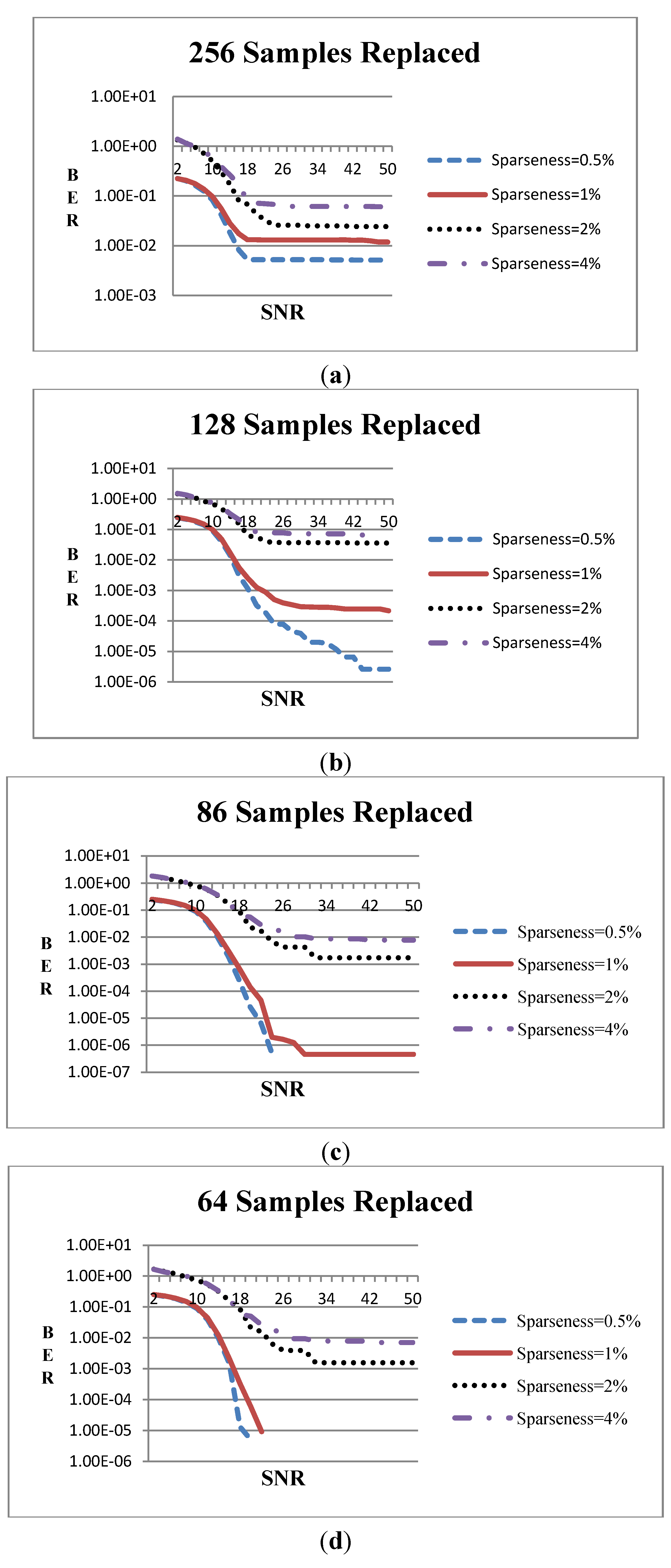
As can be seen from Figure 6 the error curves do not evolve smoothly in some cases especially when BER falls below 10−2. This is owed mainly to the high sparseness of the data. For example, if the sparseness degree is less than 2% this means that the 1536-bit packets have less than 30 bits with non zero value. When SNR is high enough (e.g., 10 dB or higher) the errors are caused by the inversion of some of these non-zero bits or the inversion of their adjacent zero bits. Thus, the error combinations are limited and therefore the BER values tend to be discrete.
In Figure 6a, 256 samples were substituted by others at the receiver for four levels of data sparseness (0.5%, 1%, 2%, or 4% of the data bits that are input to the transmitter are non-zero). The BER floor ranges between 0.005 (for 0.5% data sparseness) and 0.06 (for 4% sparseness). In Figure 6b, 128 samples were substituted and the error floor tends to be 10−6 for 0.5% sparseness when the channel SNR is adequately high. Nevertheless, there is no significant improvement when the sparseness is 2% or 4%. In Figure 6c, 86 samples were substituted and there is one case where the input is fully reconstructed (when the sparseness is 0.5%) while the error floors at the other cases are significantly improved. Finally, when 64 samples were replaced (Figure 5d), the input can be fully reconstructed when the sparseness degree is 0.5% or 1% and the channel SNR is about 18 dB.
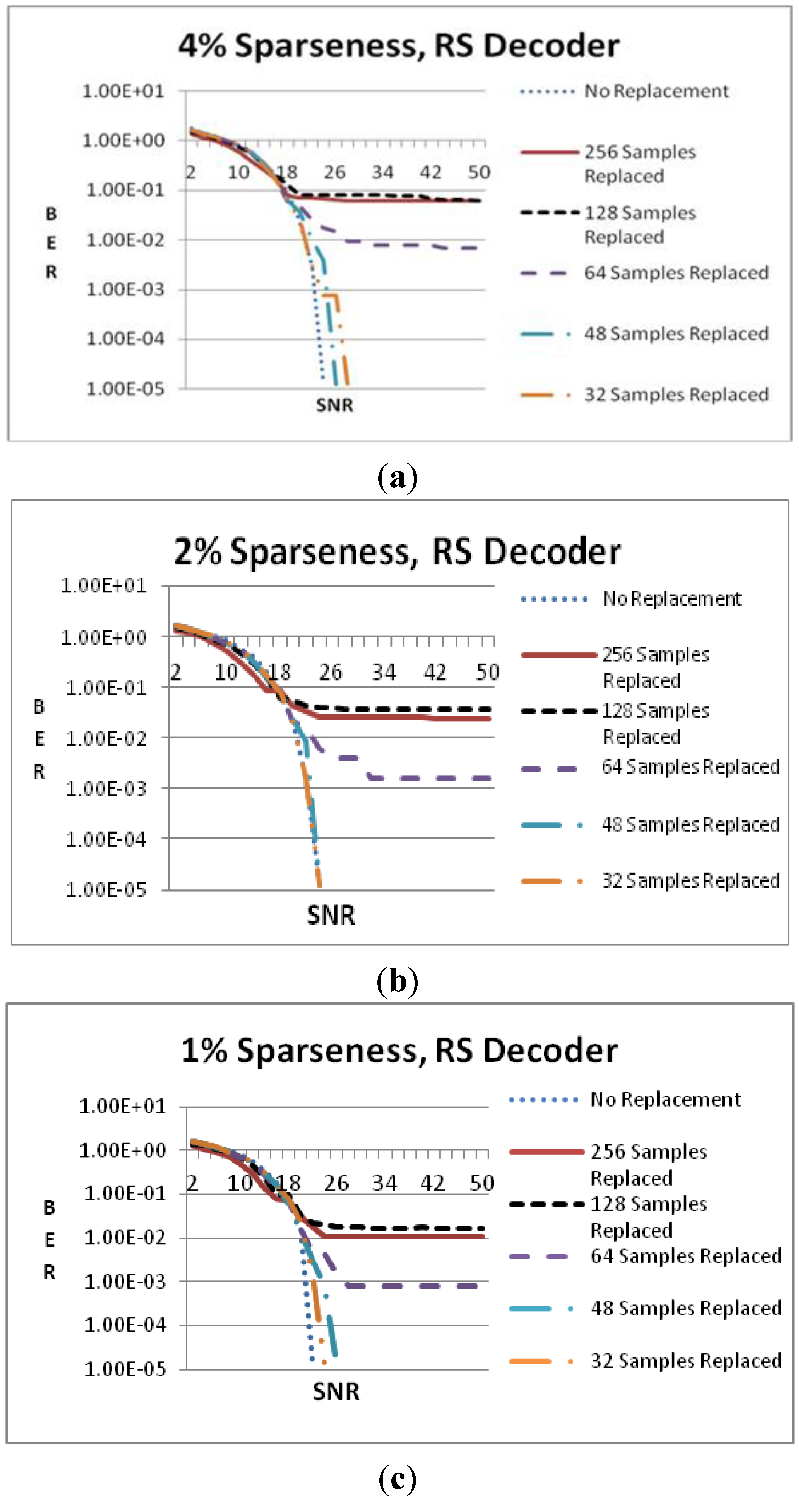
In Figure 7, a different view is given by comparing, in the same figure, the cases where different number of samples is replaced and RS decoding is used. Using RS decoder the full input signal reconstruction is possible when the data sparseness is 4% and 32 or 48 samples are substituted (see Figure 7a). The full signal reconstruction requires an SNR that is 2 or 4 dB higher than the optimal case where no samples are replaced. In Figure 7b, the sparseness is 2% and again the full reconstruction takes place when 32 or 48 samples are substituted but this occurs at the same SNR with the optimal case. The error floor at the other cases is improved compared to the case of 4% sparseness degree. In Figure 7c, 1% sparseness degree is tested but now the substitution of 64 samples does not lead to full reconstruction, as in the case of Figure 6d. Taking into consideration the exact values of the error floors in all the sparseness cases it can be stated that Viterbi decoding is more efficient than RS for the proposed undersampling scheme.
Figure 7.
BER vs. SNR when RS decoder is used and the data sparseness is (a) 4%; (b) 2%; (c) 1%.

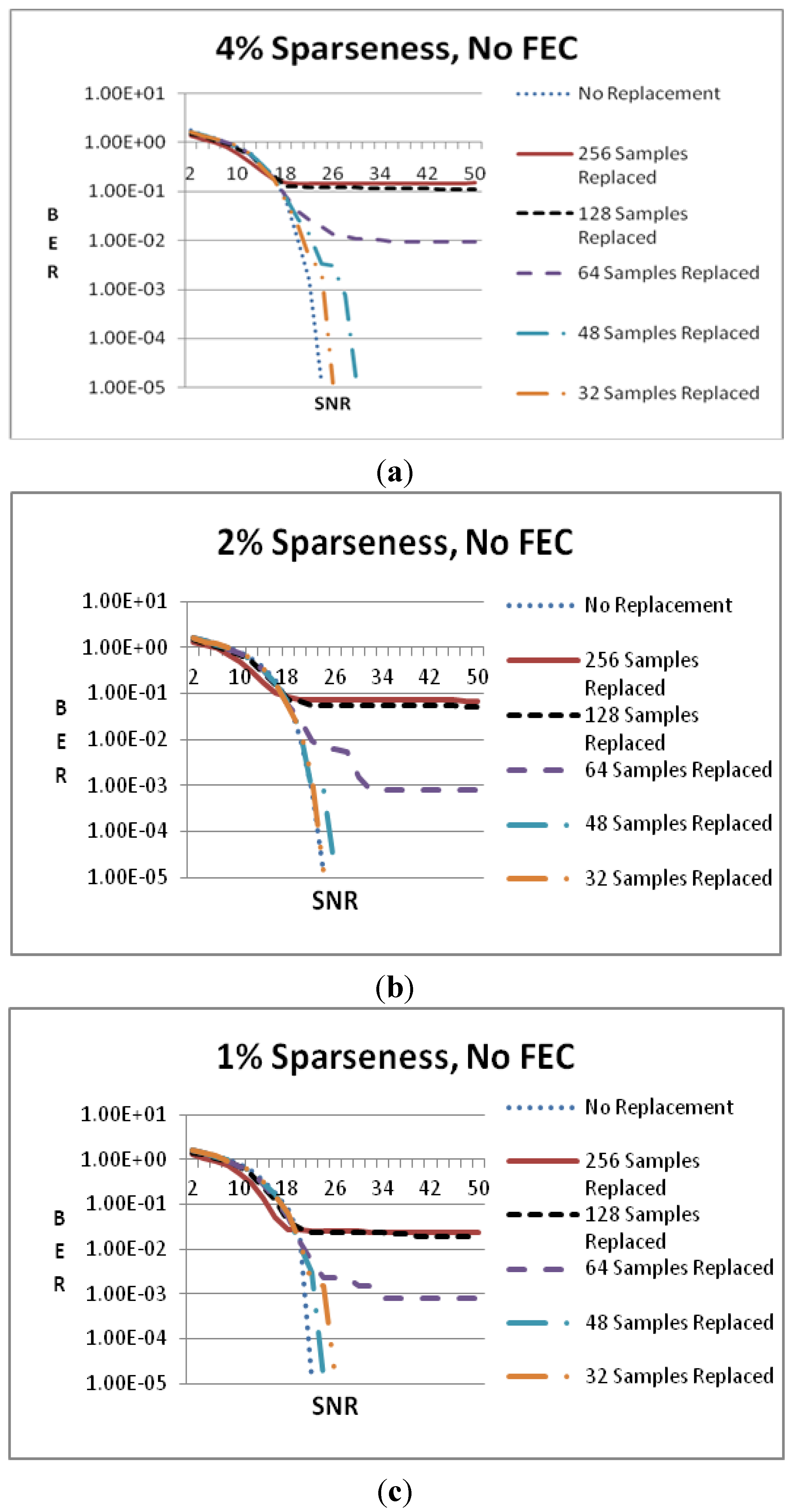
In Figure 8, similar conditions to Figure 7 are tested for the case where no FEC is employed at all. By comparing Figure 7a with Figure 8a, Figure 7b with Figure 8b, and Figure 7c with Figure 8c, it is obvious that the error floor is improved by employing an FEC method, such as RS or Viterbi. Moreover, the required channel SNR for full input signal reconstruction is lower when an FEC method is employed.
Figure 8.
BER vs. SNR when no FEC is employed and the data sparseness is (a) 4%, (b) 2%, (c) 1%.
6. Conclusions
An undersampling method that can be implemented with low complexity hardware in an OFDM environment was presented in this paper. It can reduce the samples needed at the receiver by up to 1/4 reducing the power consumption, the size of the memory needed to store the ADC samples and the complexity of the FFT. The proposed method can recover the original sparse data with zero or very low error assisted by the employed FEC scheme without the use of time consuming iterative processes.
Future work will focus on the investigation of the efficiency of different QAM modulations, FFT sizes and implementations, FEC methods, such as LDPC and Turbo Codes, interleaving schemes, etc. Different channel noise models will also be tested. Moreover, we will look for special applications where the input data obey to more sophisticated relations between them in order to allow the substitution of a larger number of samples with low BER.
Acknowledgments
This work is protected under the provisional patents with application No. 20130100014 and 20140100069 (Greek Patent Office (OBI)).
Conflicts of Interest
The author declares no conflict of interest.
References
- Kester, W. Mixed Signal and DSP Design Techniques; Newnes: Burlington, MA, USA, 2003; pp. 20–21. [Google Scholar]
- Vaswani, N. Kalman filtered compressed sensing. In Proceedings of the IEEE Int. Conf. Image Processing (ICIP), San Diego, CA, USA, 12–15 Oct 2008; pp. 893–896.
- Vaswani, N. LS-CS-residual (LS-CS): Compressive sensing on least squares residual. IEEE Trans. Sign. Process. 2010, 58, 4108–4120. [Google Scholar] [CrossRef]
- Kanevsky, D.; Carmi, A.; Horesh, L.; Gurfil, P.; Ramabhadran, B.; Sainath, T.N. Kalman filtering for compressed sensing. In Proceedings of the 13th Conference on Information Fusion (FUSION), Edimburgh, UK, 26–29 July 2010.
- Carmi, A.; Gurfil, P.; Kanevsky, D. Methods for sparse signal recovery using kalman filtering with embedded pseudo-measurement norms and quasi-norms. IEEE Trans. Sign. Process. 2010, 58, 2405–2409. [Google Scholar] [CrossRef]
- Massicotte, D. A parallel VLSI architecture of Kalman-filter-based algorithms for signal reconstruction. Integr. VLSI J. 1999, 28, 185–196. [Google Scholar]
- Massicotte, D.; Elouafay, B. A systolic architecture for kalman-filter-based signal reconstruction using the wave pipeline method. In Proceedings of the IEEE International Conference on Electronics, Circuits and Systems, Lisboa, Portugal, 7–10 September 1998; pp. 199–202.
- Candès, E.J.; Wakin, M.B. An introduction to compressive sampling. IEEE Sign. Process. Mag. 2008, 25, 25–30. [Google Scholar]
- Mishali, M.; Eldar, Y. From theory to practice: Sub-Nyquist sampling of the sparse wideband analog signals. IEEE J. Sel. Top. Sign. Process. 2010, 4, 375–391. [Google Scholar] [CrossRef]
- Mahalanomis, A.; Muise, R. Object specific image reconstruction using a compressive sensing architecture for application in surveillance systems. IEEE Trans. Aerosp. Electron. Syst. 2009, 45, 1167–1180. [Google Scholar] [CrossRef]
- Luo, J.; Xiang, L.; Rosenberg, C. Does compressed sensing improve the throughput of wireless sensor networks. In Proceedings of the IEEE International Conference on Communications, Cape Town, South Africa, 23–27 May 2010.
- Pudlewski, S.; Melodia, T.; Prasanna, A. Compressed-sensing-enabled video streaming for wireless multimedia sensor network. IEEE Trans. Mob. Comput. 2012, 11, 1060–1072. [Google Scholar] [CrossRef]
- Qi, C.; Wu, L. A hybrid compressed sensing algorithm for sparse channel estimation in MIMO OFDM systems. In Proceedings of the IEEE ICASSP, Prague, Czech Republic, 22–27 May 2011; pp. 3488–3491.
- Schniter, P. A message-passing receiver for BICM-OFDM over unknown clustered-space channels. IEEE J. Sel. Top. Sign. Process. 2011, 5, 1462–1474. [Google Scholar] [CrossRef]
- Cheng, P.; Gui, L.; Tao, M.; Guo, Y.; Huang, X.; Rui, Y. Sparse channel estimation for OFDM transmission over two-way relay networks. In Proceedings of the IEEE international conference on communications—Wireless communications symposium, Ottawa, Canada, 10–15 June 2012; pp. 3948–3953.
- Yu, J.; Boucheret, M.L.; Vallet, R.; Duverdier, A.; Mesnager, G. Interleaver design for turbo codes from convergence analysis. IEEE Trans. Commun. 2006, 54, 619–624. [Google Scholar] [CrossRef]
- Cooley, J.W.; Tukey, J.W. An algorithm for the machine calculation of complex fourier series. Math. Comput. 1965, 19, 297–301. [Google Scholar] [CrossRef]
- Biradar, P.; Uma Reddy, N.V. Implementation of area efficient OFDM transceiver on FPGA. Int. J. Soft Comput. Eng. 2013, 3, 144–147. [Google Scholar]
- Jaber, M.A.; Massicote, D. A novel approach for FFT data reordering. In Proceedings of the IEEE International Symposium on Circuits and Systems (ISCAS), Paris, France, 30 May–2 June 2010; pp. 1615–1618.
- Jaber, M.A.; Massicote, D.; Achouri, Y. A higher radix FFT FPGA implementation suitable for OFDM systems. In Proceedings of the International Conference on Electronics, Circuits and Systems (ICECS), Beirut, Lebanon, 11–14 December 2011; pp. 744–747.
- Son, B.S.; Jo, B.G.; Sunwoo, M.H.; Yong, S.K. A high-speed FFT processor for OFDM systems. In Proceedings of the IEEE International Symposium on Circuits and Systems (ISCAS), Phoenix-Scottsdale, AZ, USA, 26–29 May 2002; Volume 3, pp. III-281–III-284.
- Wey, C.L.; Lin, S.Y.; Tang, W.C.; Shiue, M.T. High-speed, low cost parallel memory-based FFT processors for OFDM applications. In Proceedings of the 14th IEEE International Conference on Electronics, Circuits and Systems (ICECS), Marrakech, Morocco, 11–14 December 2007; pp. 783–787.
- Yoshizawa, S.; Orikasa, A.; Miyanaga, Y. An area and power efficient pipeline FFT processor for 8 × 8 MIMO-OFDM systems. In Proceedings of IEEE International Symposium on Circuits and Systems (ISCAS), Rio De Janeiro, Brazil, 15–18 May 2011; pp. 2705–2708.
© 2014 by the authors; licensee MDPI, Basel, Switzerland. This article is an open access article distributed under the terms and conditions of the Creative Commons Attribution license (http://creativecommons.org/licenses/by/3.0/).
Share and Cite
MDPI and ACS Style
Petrellis, N. Undersampling in Orthogonal Frequency Division Multiplexing Telecommunication Systems. Appl. Sci. 2014, 4, 79-98. https://doi.org/10.3390/app4010079
AMA Style
Petrellis N. Undersampling in Orthogonal Frequency Division Multiplexing Telecommunication Systems. Applied Sciences. 2014; 4(1):79-98. https://doi.org/10.3390/app4010079
Chicago/Turabian StylePetrellis, Nikos. 2014. "Undersampling in Orthogonal Frequency Division Multiplexing Telecommunication Systems" Applied Sciences 4, no. 1: 79-98. https://doi.org/10.3390/app4010079