Autonomy, Conformity and Organizational Learning

1
Aix Marseille University (Aix Marseille School of Economics), CNRS, EHESS and IUF. 2 Rue de la Charité, Marseille 13002, France
2
Institute of Social Science, University of Tokyo. 7-3-1 Hongo, Bunkyo-ku, Tokyo 113-0033, Japan
*
Author to whom correspondence should be addressed.
Adm. Sci. 2013, 3(3), 32-52; https://doi.org/10.3390/admsci3030032
Submission received: 14 May 2013
/
Revised: 24 June 2013
/
Accepted: 28 June 2013
/
Published: 5 July 2013
(This article belongs to the Special Issue Computational Organization Theory)
Abstract
:There is often said to be a tension between the two types of organizational learning activities, exploration and exploitation. The argument goes that the two activities are substitutes, competing for scarce resources when firms need different capabilities and management policies. We present another explanation, attributing the tension to the dynamic interactions among search, knowledge sharing, evaluation and alignment within organizations. Our results show that successful organizations tend to bifurcate into two types: those that always promote individual initiatives and build organizational strengths on individual learning and those good at assimilating the individual knowledge base and exploiting shared knowledge. Straddling the two types often fails. The intuition is that an equal mixture of individual search and assimilation slows down individual learning, while at the same time making it difficult to update organizational knowledge because individuals’ knowledge base is not sufficiently homogenized. Straddling is especially inefficient when the operation is sufficiently complex or when the business environment is sufficiently turbulent.
1. Introduction
I think our growth will end at only two or three times the current scale, once we undertake to increase routines. I think the biggest reason we don’t see “mega ventures” emerging in Japan is that every firm starts organizing and routinizing their processes too early. When I worked with American firms, such as Microsoft or Apple, I was always surprised to see disorder in many aspects of their operations. They would not be called “firms” if they were in Japan. Their processes are not very routinized, but that is exactly why they can continue to grow. Their workplaces are full of chaos, especially compared to their Japanese counterparts. However, creative people who can make breakthroughs prefer working in such places. So it is with our company. We are paying the cost of disorganization and mistakes caused by the chaos…but, it is impossible to have both creative workers and routine workers in the optimal mix.- Masayuki Makino, CEO, Works Applications, Inc. [1]
The tension between exploration and exploitation has been a central theme in the literature on organizational learning since the work of March [2]. The issue is not simply academic, but a real problem faced by many business executives, as expressed by the CEO of one of Japan’s fast-growing business software companies quoted above. However, few theories have been developed to analyze the trade-offs creating this tension at the organizational level. In this article, we propose an agent-based model that formulates what we believe are four important steps allowing organizational learning: search, knowledge sharing, evaluation and alignment. The model sheds light on the sources of the primary tension between exploration and exploitation by focusing on the development of organizational knowledge, i.e., the set of ideas that are institutionalized in the form of systems, structures, strategies and procedures.
We identify search and assimilation as the two main drivers of knowledge development and exploitation. Assimilation is taking in organizational knowledge as one’s own. High conformity to organizational knowledge facilitates its upgrading, which, in turn, accelerates exploitation in our model. Key to our model is the idea that knowledge diversity (i.e., diversity in individuals’ knowledge) makes searching more effective, but impedes the updating of organizational knowledge, thus creating an obstacle to its exploitation. Although March [2] argues that efforts to exploit existing knowledge eventually suppress exploration by reducing the diversity of knowledge, he does not illustrate the opposite mechanism: exploration itself makes exploitation difficult. The mechanism we illustrate in this paper goes beyond the usual argument that exploration and exploitation compete for scarce resources [2,3]. Our model suggests that the tension between exploration and exploitation does not necessarily come from resource constraint (which is also present in our model), but rather from the tendency for too diverse knowledge to lead people to disagree on how their ideas and activities should be aligned.
We develop a model of organizations that undertake tasks of varying degrees of complexity. The complexity of a task is formulated as interdependency among tasks in determining functional performance following the NK landscape model [4]. We also introduce environmental turbulence by allowing the performance function to be redefined randomly from time to time. The NK landscape has been applied in the literature on organization theory. In their series of papers, Rivkin and Siggelkow consider how to design a decision-making process in hierarchical (or multi-level) organizations undertaking complex projects in turbulent environments [5,6,7,8]. In particular, they sought to understand the relationship between the levels of decision-making when lower layers in a hierarchy have narrower scope. The same aspects are considered by Barr and Hanaki [9]. For example, Rivkin and Siggelkow [5] demonstrate that interdependencies are formed among elements of organizational design (such as the allocation of real decision authority and the design of performance measures), underlying technology and manager ability, because of the tension between the need for broad search and the need for stabilizing around good decisions. In other words, organizational elements that enable discovery may undermine lock-in to good solutions. Other applications of the NK landscape in management literature include, for example, Gavetti and Levinthal [10] and Marengo and Pasquali [11]. Gavetti and Levinthal [10] consider the interplay between a forward-looking “off-line” search and a backward-looking “on-line” search and their implications for organizational performance. Marengo and Pasquali [11] consider the interaction between incentives and allocation of decision rights and show that a principal can obtain the desired outcome either by providing appropriate incentives or by appropriately allocating the decision rights to agents. Our analysis departs from the existing literature on agent-based models in two respects: (1) we do not consider hierarchical organization; and (2) the focus of our analysis is the dynamic interaction between individual search and organizational learning. What is surprising about our findings is that the optimal parameter choices are bimodal—either full autonomy or a high level of organizational conformity. This indicates that the tension between exploration and exploitation may not be a question of simple trade-offs, as assumed for search and stability in Rivkin and Siggelkow [5], but rather that it may be driven by the dynamic interaction between agents’ knowledge search and their knowledge assimilation process.
There are two important assumptions that drive the key results in our theory. First, we assume that updating organizational knowledge requires a certain level of consensus. In our model, organizational knowledge is successfully updated only when a majority of high performers agree with the proposal to change it. Therefore, merely sharing new ideas with others is not enough to ensure implementation at the organizational level: many others must have a similar view of the world and attach the same meaning to the idea. This means that a certain level of organizational homogeneity is required to promote organizational learning.
Second, we assume that the organization’s management influences time allocation between exploration (i.e., experimenting with new ideas) and exploitation (i.e., copying organizational knowledge) at the individual level. An example is the famous story of 3M’s mandatory rule that its technical people should be able to devote 15% of their time to any projects of their own choice, rather than those they are officially assigned to. Management can encourage exploration by developing a culture that emphasizes autonomy, but it can also induce exploitation by setting up an information-sharing structure and developing monitoring and incentive systems that encourage people to conform to existing organizational knowledge.
Regarding the first assumption, March [2] includes a similar feature, namely, the updating of organizational knowledge is less frequent in the dimensions where there is less consensus among high performers. However, our model specification better captures the cost of knowledge heterogeneity—an impediment to organizational learning—and we are not aware of any existing research that formally examines the effect of organizational conformity in a model where agents search among multiple locally-best configurations.
Through extensive simulations using the model, we find that (1) frequent knowledge sharing within an organization has positive effects on its performance; (2) there are non-monotonic relationships between degree of autonomy (or conformity) and organizational performance; and (3) either when tasks are complex or when the environment is turbulent, successful firms tend to bifurcate into two types: those that always promote individual initiatives and build organizational strengths on individual learning and those good at assimilating individuals’ knowledge base and exploiting shared knowledge. We will call the former high-autonomy organizations and the latter high-conformity organizations. This bifurcation is similar to findings by Levinthal and March [12] and Ghemawat and Ricart i Costa [13] showing that organizations tend to wind up with “extremes” in the presence of non-concavity in the optimization problem. Although individuals allocate a small portion of their time to search in the high-conformity organization, they quickly accumulate organizational knowledge, because their assimilated knowledge base helps them to agree on whether a new idea is good or bad.
It is rather intuitive that too much assimilation of knowledge (too little autonomy) is counter-productive, because without diversity in the search for better solutions, neither individual knowledge or organizational knowledge will improve. However, it is less obvious why straddling the high-autonomy and high-conformity types of organizations fails when the operation is sufficiently complex or the business environment sufficiently turbulent. The intuition is as follows: on the one hand, a hybrid organization (i.e., with more equal allocation of time between individual search and assimilation of knowledge) experiences slower individual learning through search than does the high-autonomy organization, where 100% of time is allocated to individual search. On the other hand, a moderate level of individual search means that individual knowledge is too diverse for an organization to update knowledge effectively. In such organizations, once members reach locally-best solutions at the individual level, they cannot agree on how to improve the organizational knowledge. We find that this slow evolution of organizational knowledge is more costly when tasks are interdependent (complex, in our terminology) or when the environment continually changes (is turbulent).
The dynamics of these two potentially optimal organizations also differ. Our findings reveal that the performance of the high-autonomy organization is always better than that of the high-conformity organization, initially. When the task becomes sufficiently complex or when environmental turbulence becomes sufficiently high, however, the latter catches up with the former, outperforming in later periods. This reversal of performance is due to the difference in the rate at which organizational knowledge improves. In the high-conformity organization, since individuals’ knowledge is assimilated through high conformity to organizational knowledge, their search is more aligned and organizational knowledge improves steadily. This finding is somewhat similar to the recent findings in the experimental economics literature, where Kocher and Sutter [14], Cooper and Kagel [15] and Bornstein et al. [16] show that, while initially, teams may not perform better than individuals, they learn how to adopt and use strategic reasoning faster in the underlying games.
Our work differs from the group diversity literature in organizational behavior, which generally finds that diversity in functional experience and information sources improves group performance [17,18,19,20]. Our model assumes that agents have uniform behavior and capability and, thus, presumes no effect of functional diversity. Gains from knowledge sharing only come from faster learning, due to improved organizational knowledge under the assimilation of individuals’ knowledge. Conversely, diversity in the individual knowledge base impairs organizational learning due to inability to agree on how to update organizational knowledge, resulting in the tension observed between exploration and exploitation.
Crossan et al. [21] expressed a view similar to ours in their attempt to develop a conceptual framework: “This tension (between exploration and exploitation) is seen in the feedforward and feedback processes of learning across the individual, group, and organization levels.” According to them, feedforward is the transference of learning from individuals and groups to the organizational levels, where ideas are embedded in the form of systems, structures, strategies and procedures. Feedback is the way in which this embedded or institutionalized learning affects individuals and groups. Note that in our model, the feedback process comes into the notion of exploitation, where development of organizational knowledge assimilates learning and actions at the individual level. However, although our view is similar to that of Crossan et al. [21], the tension arises endogenously in our model, whereas it is assumed as one of the four key premises in their framework ([21], p. 523).
2. Model
Consider an organization that consists of M agents. Each agent undertakes an identical task having N dimensions. The value that an agent generates depends on how the agent configures each dimension of the task. The performance of the organization depends on the values generated by the agents therein.
Let be agent i’s configuration of dimension j in period t, and becomes i’s configuration of the task in period t. The corresponding value agent i generates or the performance of agent i in period t is . The performance of the organization in period t, , is defined simply as the mean performance of its members, i.e., The assumption that each dimension can be either zero or one is made for the sake of simplicity. The model can be easily extended so that a dimension can be configured in many ways. If the number of possible configurations of a dimension is c, then the number of possible configurations of the task becomes
We formulate the performance function, , based on the Landscape model [4], which allows us to parameterize the interdependencies among N dimensions with a parameter, K. Namely, the ideal configuration for dimension j depends on i’s configurations of K other dimensions. We assume that these K dimensions are chosen randomly from other dimensions. There are many other possible structures of interdependencies. Rivkin and Siggelkow [6] demonstrate that the structure of interdependencies, even controlling for K, affects the complexity of the environment and the effectiveness of various search strategies. Let be the set of these K dimensions that affect the effectiveness of and be i’s configurations of these K dimensions in period t. Then:
where is defined by assigning values drawn randomly from to each possible and . Every agent faces the same performance function, or .
When modeled in this way, the number of possible configurations of the task is , a potentially large space in which agents must search for better configurations. The parameter K captures the complexity of the task. When , there is no interdependency among dimensions; thus, changing the configuration of one dimension results in smooth changes in performance. The larger K is, the more interdependencies there are among different dimensions. When K is large, changing the configuration of one dimension has a non-additive effect on the value generated by the agent.
To capture the possibility of instability of the environment in which organizations operate, we introduce a parameter, , such that, in each period and for each possible configuration of task, X, is redefined randomly to a value drawn from , with probability μ. When μ is zero, the values associated with each possible configuration of the task remain constant over time. When the value of μ is higher, these values can change quite drastically from period to period; thus, the environment will be turbulent. We now turn to how the behaviors of organizations are modeled.
2.1. Search, Learning and Organizational Conformity
We assume that each agent receives a randomly configured task initially; i.e., are randomly set for all i and j. Agents modify their configurations over time by conducting individual searches and by learning from the organizational knowledge. Let denote the organizational knowledge at period t where represents the organizational knowledge of dimension j at period t. We assume that is randomly set. We allow the organizational knowledge itself to evolve over time as agents in the organization contribute their knowledge in the manner described below. Note that knowledge sharing improves organizational performance because agents face the same .
In each period, each agent either conducts an individual search for a better configuration (with probability λ) or learns from the organizational knowledge (with probability ). The individual searches are conducted as follows: an agent chooses one of the N dimensions randomly and ascertains whether changing its configuration generates a greater value. If it does, he adopts the change. Otherwise, his configuration remains as before.
When an agent learns from the organizational knowledge, he randomly chooses a dimension, such that his current configuration differs from that of the organizational knowledge, and then adopts the organizational knowledge for the chosen dimension. Copying a part of the organizational knowledge in this manner gradually assimilates the individual knowledge base to the organizational knowledge if λ is sufficiently low. As we explain later, the harmonized knowledge base facilitates upgrading of the organizational knowledge. When adopting the configuration from the organizational knowledge, the agent does not check whether doing so generates a higher value. When λ is less than one, we assume that the organization’s management is using a monitoring and incentive mechanism to ensure the assimilation of the individual knowledge base, meaning that the process of assimilation can also be interpreted as organizational control.
When λ is low, agents tend to follow the configurations of the organizational knowledge; thus, all their practices are aligned. Conversely, when λ is high, since the search is individual, agents’ configurations may remain diverse. Therefore, parameter λ represents their degree of autonomy (i.e., high λ indicates high individual initiative and low organizational control). The issue is the relationship between degree of autonomy and organizational performance under various levels of complexity and turbulence.
At the end of each period, with probability p, each agent proposes to modify the organizational knowledge. He does so by randomly choosing one dimension, such that his configuration differs from that of the organizational knowledge, and by proposing to change the configuration of the chosen dimension in such a way that it matches his current configuration. Whether the proposal is accepted or not depends on its support from agents in the organization. It is accepted if the majority of the agents whose performance is no less than the performance of the organization configure the dimension as proposed. That is, we consider the majority of those agents k, such that . In the case of a tie, a proposal is approved with probability . Parameter p can be interpreted as the frequency of knowledge sharing within the organization. The higher the value of p, the more quickly organizational knowledge improves.
The model presented here is similar to that of March [2]. In particular, both our model and that of March [2] consider learning within an organization through updating the organizational knowledge and assimilation of individual knowledge to the organizational knowledge. March [2] considers such an assimilation process as the result of “socialization” among individuals. Our model differs, however, from that of March [2] in its assumption regarding individual search, the underlying configuration space, and the way the organizational knowledge is updated. Firstly, individuals do not actively search for the ideal configuration in March [2], while they do in our model. Secondly, March [2] assumes the existence of a unique configuration that an organization needs to discover, and performance is measured according to distance (in terms of number of dimensions that differ) from the ideal configuration. In contrast, our model employs the NK landscape in determining performance, and there can be many distinct locally-best configurations when a task is complex. Thirdly, March [2] assumes that the updating of organizational knowledge is possible, even when only a small minority of high performers share the view, albeit with a lower probability, whereas in our model, agreement by a majority is required to change organizational knowledge.
3. Results
There are six parameters in our model. The task is defined by its size, N, and its complexity, K. Environmental turbulence is captured by μ. The organization is characterized by the number of agents, M, the frequency of knowledge sharing among them, p, and the degree of autonomy, λ. In all the simulations, we fix N and M at 100 and 20, respectively, and vary other parameters to investigate the effect of autonomy/conformity and frequency of communications on the performance of organizations under various degrees of complexity and turbulence. Appendix shows the results from and , which are similar to the results from .
For each set of parameter values, the payoff function, , initial configuration for individual tasks, , and organizational knowledge, , are generated. Then, we allow organizations to operate in the manner described in the Model section for 1,000 periods. Table 1 shows the pseudo code of the simulations.

| 1. | Set parameter values and give a random seed | ||
| 2. | Initialize NK landscape, agents and organizational knowledge | ||
| 3. | For | ||
| (a) | For each agent, | ||
| (i) | Search (λ) or copy () | ||
| (ii) | Update the agent’s configuration and performance | ||
| (b) | Update performance of organization | ||
| (c) | For each agent, (in random orders) | ||
| (i) | Proposes (with probability p) or not. | ||
| (ii) | If proposes, evaluate the proposal | ||
| (iii) | Update organizational knowledge | ||
| (d) | If , update NK landscape, the performances of agents and the organization | ||
| (e) | Back to (a) | ||
To summarize the performance of an organization over time, we mainly focus on present discounted values (PDVs) of organizational performance over these 1,000 periods: namely, , where δ is a discount factor. Below, we will set the discount factor at . This discount factor gives the payoff for the last period a weight that is 0.37 of that for the first period. If we set the discount factor too low, the payoff at will be given a negligible weight compared to those for earlier periods. For example, if , the weight for the payoff at will be less than of the payoff at . Since performance can take a long time to level off, we want the weight of payoff at to compare favorably with the initial payoffs. We will discuss the effect of changing the value of δ in light of the dynamics of organizational performance below. We also take an average over 500 simulation runs based on varying random seeds, to ensure that our results are not driven by a few special realizations of our simulation.
Before turning to the outcomes of the model simulation, let us briefly discuss the basic property of the NK landscape. It has been shown by Kauffman [4] that when and , the performance function defined by the NK landscape has a unique locally-best configuration (thus, it is also the globally best configuration). Furthermore, it has been shown that local search processes, such as the one we consider in our individual search process, will eventually find the best configuration. Thus, for and , differences in performance among organizations with varying values of p and are simply due to their speed in finding the best configuration. When , on the other hand, the NK performance landscape has various local maxima, and local search processes can get stuck with a configuration that corresponds to one of these local maxima and, therefore, fail to find the globally best configuration. When , the best (locally, as well as globally) configuration changes from time to time. Thus, how fast the right configuration can be found in a changing environment becomes crucial. Keeping this basic property of the NK landscape in mind will help clarify the results that we turn to now.
3.1. Effect of p and λ
Figure 1 shows the PDV (by height) for various degrees of activeness of communication, p (the horizontal axis), and of autonomy, λ (the vertical axis), under four combinations of complexities, , and uncertainties, . Recall that a higher λ represents weaker organizational conformity.
Figure 1.
Average present discounted values (PDVs) of organizational performances for various p and λ in four combinations of task complexity ( (left) and (right)) and environmental turbulence ( (top) and (bottom)). Discount factor is . Data are generated by taking an average over 500 simulation runs for each set of parameter values.
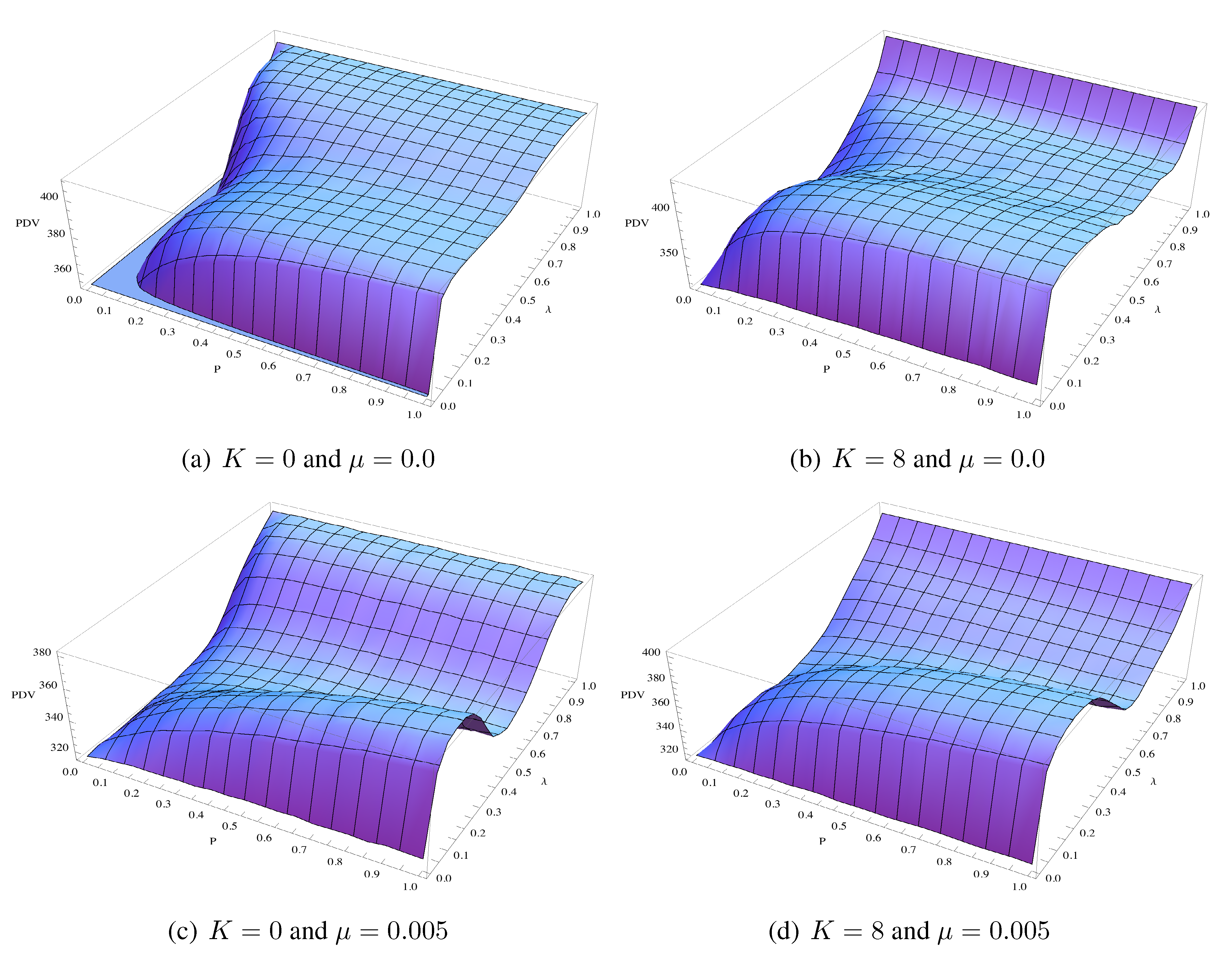
All four panels in Figure 1 show that organizational performance as measured by PDV improves as the communication becomes more active (i.e., as we move along the horizontal axis from low to high p). That is, the more frequently individuals engage in knowledge sharing, the higher their organizational performance, regardless of task complexity and environmental uncertainty.
While the figure exhibits a monotonic relationship between PDV and frequency of knowledge sharing, p, the relationship between PDV and autonomy, λ, is not monotonic in three out of four cases shown in Figure 1. When the task is complex or the environment is turbulent (Panel (b)-(d)), the optimal parameter choices for λ are bimodal—either full autonomy or a high level of organizational conformity.
Let us first consider the case in which there is a monotonic relationship between PDV and λ. This is true when the task is simple () and the environment stable () (Panel (a)). In this case, a higher λ leads to a higher PDV, although PDV quickly levels off beyond when p is sufficiently high. This result comes from the the property of the NK landscape for and : all individuals in the organization eventually find the unique locally-best (as well as globally best) configuration through their individual search. Forcing them to confirm to organizational knowledge by choosing low λ slows down the search at the individual level (because agents search less often), but the loss from the slow search is limited when organizational knowledge is improved sufficiently rapidly (i.e., when p is high enough). Since the agents’ knowledge becomes homogeneous even without any information sharing (i.e., all approach the unique best configuration), the knowledge heterogeneity in the initial state does not greatly impede organizational learning.
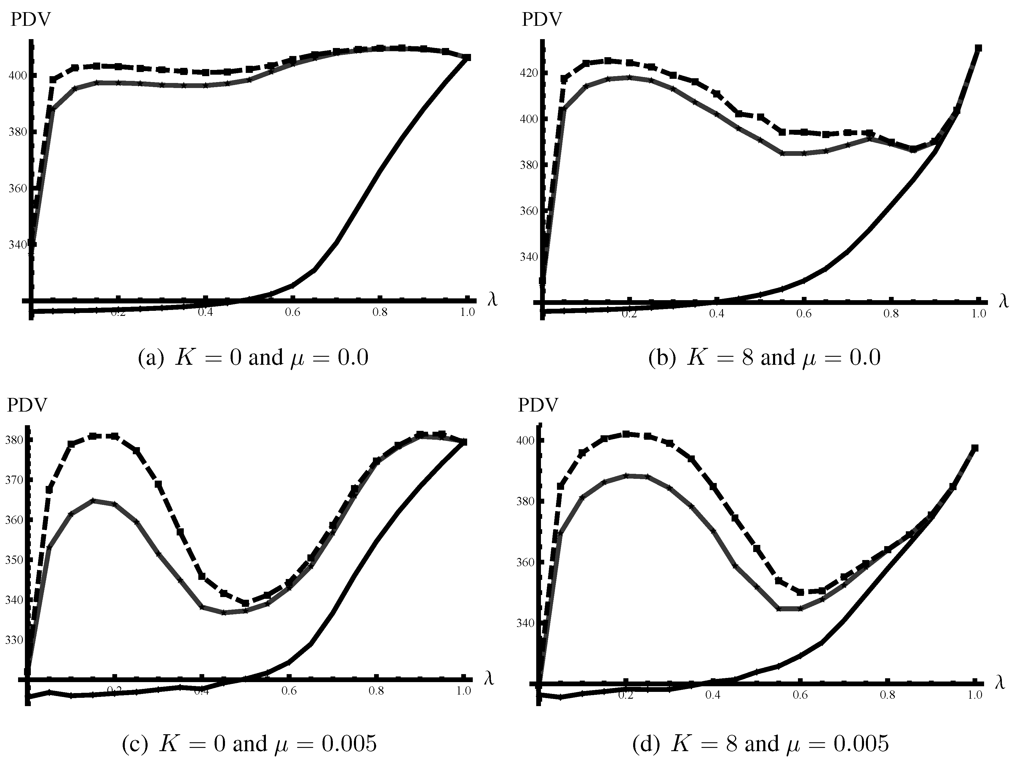
In the remaining three cases shown in Panel (b), (c) and (d), the relationship between PDV and λ is non-monotonic when the level of knowledge sharing in the organization, p, is sufficiently high. In these cases, the performance of the organization has two peaks: (1) when autonomy is very high, i.e, (the high-autonomy organization); and (2) when there is a substantial, but not overly-strong, organizational conformity, (the high-conformity organization). When λ is very small (so that individual searches are seldom conducted) or has intermediate values of around 0.5 or 0.6, performance becomes low. See Figure 2 for cross section views of Figure 1 at , and where the locations of peaks are better illustrated. It can also be seen from the figure that for to generate as high a level of performance as , the knowledge-sharing efforts must be persistent (i.e., sufficiently close to ).
Why do successful organizations, in the face of complex tasks and turbulent environments, bifurcate into two types? In other words, why do we obtain non-monotonic relationships between λ and organizational performance? To answer this question, we turn to the dynamics of performance in the next subsection.
Figure 2.
Average PDVs of organizational performances for various λ in four combinations of task complexity ( (left) and (right)) and environmental turbulence ( (top) and (bottom)). In each figure, results for three distinct ps are reported: (solid black), (solid gray) and (dashed black). The discount factor is . Data are generated by taking an average over 500 simulation runs.

3.2. Dynamics
In this subsection, we show that when the task is complex or the environment turbulent, (1) choosing the intermediate level of λ substantially slows down both individual and organizational learning; and (2) high-autonomy organizations tend to outperform high-conformity organizations, initially, although the latter eventually outperform the former. Figure 3 shows the evolution of organizational performance over time for four values of λ, (shown in solid black, solid gray, dashed black and dashed gray, respectively) and for the four combinations of and . These four λs are chosen, because they correspond approximately to the local maxima and minima of organizational performance measured by PDV. Knowledge sharing within an organization is assumed to be very frequent, . As we have seen above, a lower value of p results in lower performance for an organization with λ lower than one. Figure 3 reports the average per-period organizational performance for each block of 100 periods, i.e., for , , and so on.
Figure 3.
Average performance over time for two levels of complexity, (left) and (right) and two degrees of environmental turbulence, (top) and (bottom). Four values of λ are considered: (solid black), (solid gray), (dashed black) and (dashed gray). The communication is active (). The data is generated by taking the average per period organizational performance for each block of 100 periods. The average from 500 simulation runs is reported.

When the task is simple and the environment stable (i.e., and ), organizations with high autonomy (i.e., higher λs) improve their performance faster (Panel (a)). As discussed above, the best configuration for the task can be found through the particular local search process considered in this paper. Therefore, all the agents in an organization will eventually find the unique best configuration as long as . (Note that when , there is no individual search, so agents never find the best configuration). Once everyone in an organization has found the best configuration, there is no further improvement in organizational performance. Organizations with the highest autonomy that conduct only individual searches () do not necessarily outperform organizations with higher levels of conformity (), because the latter organizations can achieve very good performance, provided knowledge sharing takes place frequently enough. As knowledge sharing becomes less frequent (i.e., lower p), however, the higher conformity imposed on individuals (i.e., lower λ) does tend to hinder individual searches and impair organizational performance.
When the task is complex, the results are quite different, even in the complete absence of environmental turbulence. Panel (b) of the Figure 3 shows that a higher value of λ corresponds to a higher performance only in the early periods, namely the first 100 periods. In later periods, for example, for , while (dashed gray) exhibits the highest performance, the performance of (dashed black) is lower than that of (solid gray). Eventually, outperforms . This case demonstrates the possible trade-off between performance in earlier periods and performance in later periods. This reversal in relative performance between high-autonomy organizations and high-conformity organizations during 1,000 periods makes it clear that we should not set δ too low. If we set δ too low, the better performance of high-conformity organizations in the later periods will not be captured in PDV. On the other hand, we want to avoid , because if the simulation were much longer, this would hide the high performance in early periods when computing PDV. It should also be noted that the average performances in all three cases, except for , converge to the same level in the final 100 periods of our simulations, as shown in Panel (b) of the figure.
In turbulent environments (Panels (c) and (d)), the performances of the organizations with and exhibit a similar pattern to that shown in Panel (b). That is, initially, the organization with demonstrates higher performance than the organization with , but in the later periods, the latter outperforms the former. However, the dynamics of performance for (solid black) is quite different in turbulent environments from that in stable environments. That is, when the environment is sufficiently turbulent, performance does not improve much over time (in the case of a complex task, Panel (d)) or can even deteriorate (in the case of a simple task, Panel (c)). Note that, due to environmental turbulence, organizational performance in an individual simulation run demonstrates high temporal variations. Such volatilities are hidden, however, in Figure 3, where we plot the averaged performance in each block of 100 periods and further take averages across 500 simulation runs. Nonetheless, deterioration of average performance appears for after period 200 for and (Panel (c)). This puzzling outcome deserves more careful analysis.
How could the performance for in a turbulent environment with a simple task deteriorate after an initial improvement? Looking at the dynamics of diversity of individual configurations, measured by the average distance between individual configurations and their means, and the dynamics of the value of organizational knowledge, , helps us to answer this question. Let us first define the diversity of individual configurations more precisely. The mean configuration of dimension, j, at period, t, is . The distance between configurations of individual, i, and the mean configurations at period, t, is therefore . The diversity for an organization in period, t, is .
The dynamics of diversity of individual configurations is plotted in Figure 4, and the dynamics of the value of organizational knowledge in Figure 5, for four combinations of task complexity, , and environmental turbulence, . is assumed.
Figure 4.
The diversity within an organization for two levels of complexity, (left) and (right), and two degrees of environmental turbulence, (top) and (bottom). The communication is active (). Four values of λ are considered: (solid black), (solid gray), (dashed black), (dashed gray). For clarity of exposition, only are shown in the main figure. See the insets for all four λs. The extent of diversity is measured based on the discrepancy between individual configurations and their means. The data is generated by taking the average per-period diversity for each block of 100 periods. The average from 500 simulation runs is reported.
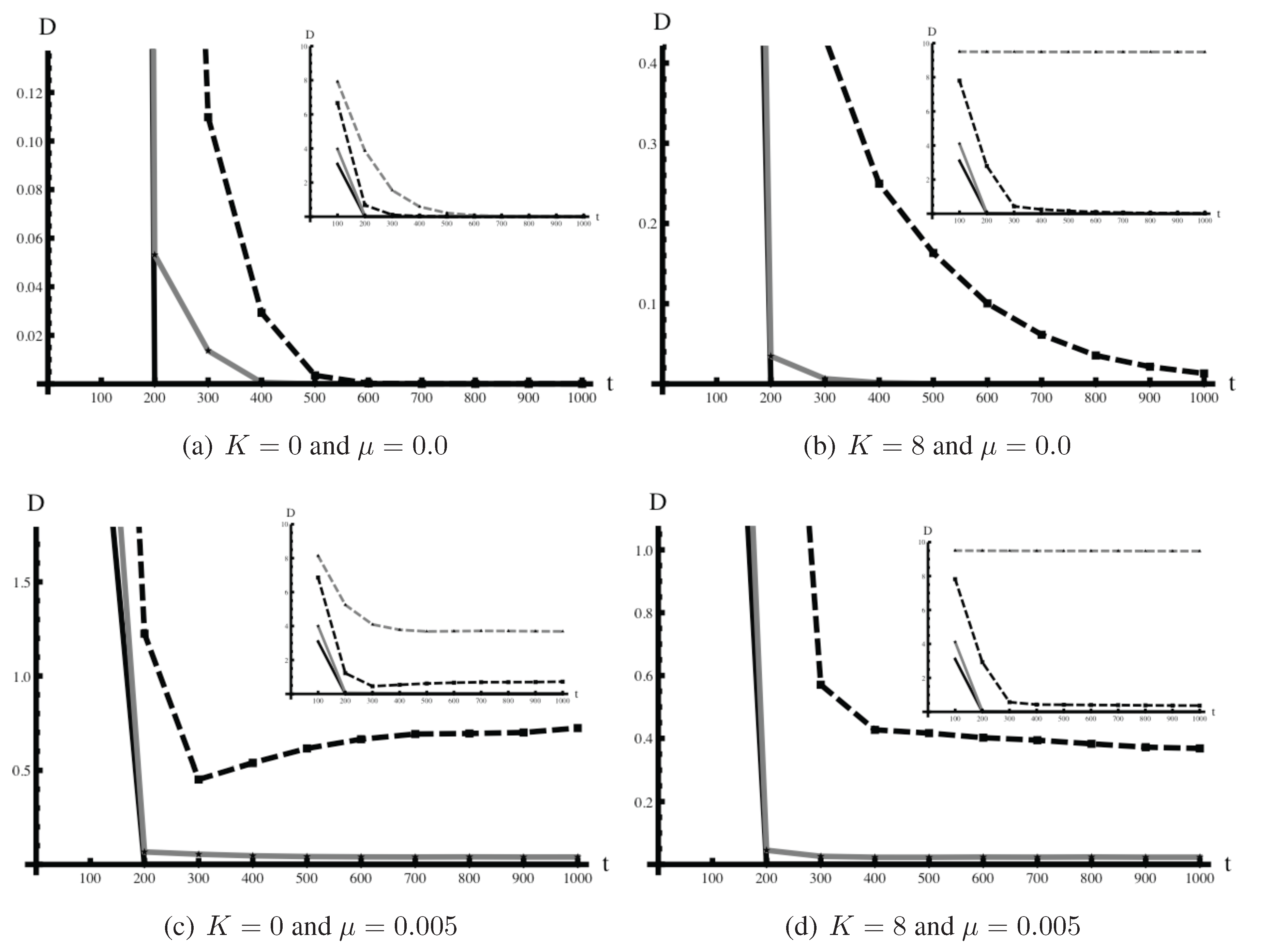
As in the case of organizational performance shown in Figure 3, we took the average over each block of 100 periods. Figure 3 reports the results obtained from taking the average of these averaged per-period performance results across 500 simulations. For clarity of exposition, in each panel of Figure 4, the diversity measures of individual configurations for are shown in the main figure and the diversity for is shown only in the in-set (together with the other three)
When the task is simple and the environment stable, the diversity measure converges to zero for all types of organizations plotted in Figure 4 (Panel (a)). The lower λ is, the faster the convergence. The reason why even an organization with (dashed gray, shown only in the in-sets) shows zero diversity in the later period is that, as discussed above, when and , every agent in the organization eventually finds the unique best configuration through individual searches. Moreover, since everyone eventually agrees on the best configuration, the value of organizational knowledge shows rapid improvement, as shown in Figure 5 (Panel (a)).
Figure 5.
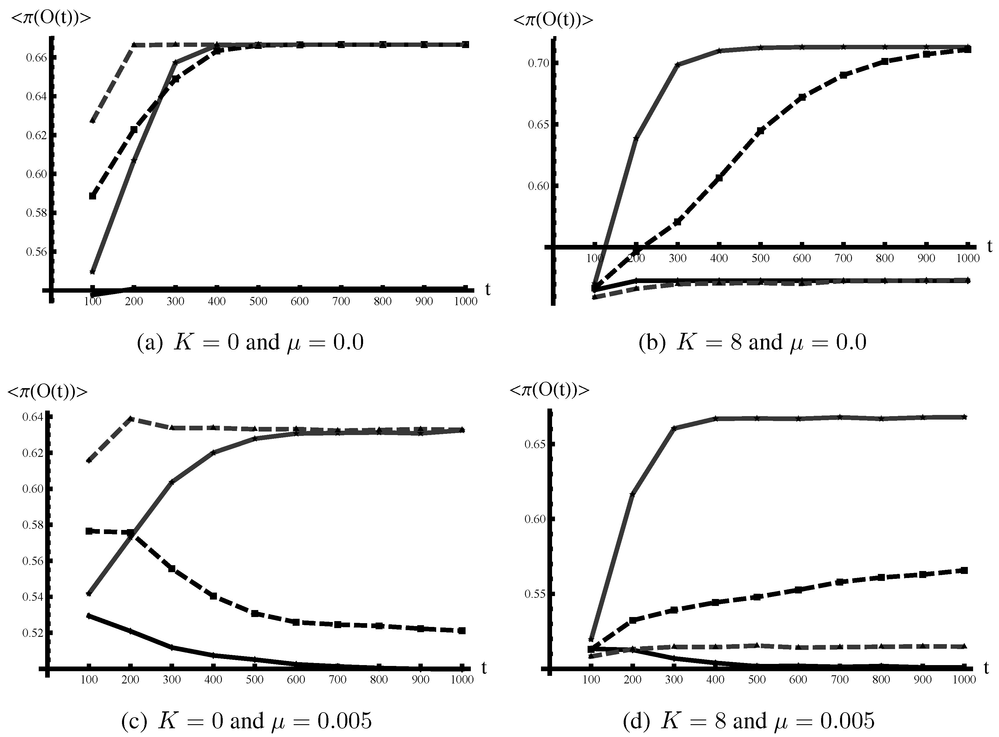
The dynamics of the average value of organizational knowledge for two levels of task complexity, (left) and (right), and two degrees of environmental turbulence, (top) and (bottom). Four values of λ are considered: (solid black), (solid gray), (dashed black), (dashed gray). The communication is active (). The data is generated by taking the average per-period value of organizational knowledge for each block of 100 periods. The average from 500 simulation runs is reported.
Figure 5.
The dynamics of the average value of organizational knowledge for two levels of task complexity, (left) and (right), and two degrees of environmental turbulence, (top) and (bottom). Four values of λ are considered: (solid black), (solid gray), (dashed black), (dashed gray). The communication is active (). The data is generated by taking the average per-period value of organizational knowledge for each block of 100 periods. The average from 500 simulation runs is reported.
When the environment is stable, but the task complex (, ), as shown in Figure 4 (Panel (b)), diversity remains high for organizations with (dashed gray, shown only in the in-set) for long periods of time, while the diversity measures in the organizations with and quickly converge to zero. When , the diversity measure declines much more slowly than with smaller values of λ.
The high diversity found for organizations with under the complex task is due to the existence of many distinct, but locally-best, configurations. Since such locally-best configurations vary, diversity among the individual configurations remains high and agents in the organizations do not agree on how to improve organizational knowledge. As a result of this dissonance in individual knowledge, the value of organizational knowledge remains low (Figure 5, Panel (b)).
Panel (b) of Figure 5 also shows that an organization with is much slower at improving organizational knowledge than one with . Recall that, in our model, in order to modify organizational knowledge, not only must new proposals be submitted, they must also be approved. In the model considered here, a proposal is approved when a majority of better-performing agents configure the dimension as proposed. Also, as discussed above for the case of , when a task is complex, individual searches may lead to various distinct configurations that are local optima. If many agents search in different directions, it is more difficult for them to agree on how to modify organizational knowledge. The insufficient alignment of the individual knowledge base resulting from lower assimilation creates a bottleneck to improvement of organizational knowledge, which, in turn, slows down the improvement of organizational performance.
The inability to improve organizational knowledge can be detrimental when the environment is changing. As shown in Panel (c) of Figure 5, an unstable environment, even in the absence of any interdependencies (i.e., a task is not complex), could prevent organizational knowledge from improving. When , an intermediate level of conformity, the quality of organizational knowledge deteriorates over time, especially after the first 100 periods. This lack of effective organizational learning is caused by the persistent diversity of individual knowledge—depicted in panel (c) of Figure 4—that prevent agents from agreeing how to update the organizational knowledge. This explains why the average performance in organizations with deteriorates, as can be seen in Panel (c) of Figure 3. Interestingly, when organizations face both complex tasks and turbulent environments, a high-conformity organization (i.e., ) improves its organizational knowledge much faster than any other organization type, as shown in Panel (d) of Figure 5. Although a high-autonomy organization (i.e., ) is incapable of improving organizational knowledge in this case, in marked contrast with Panel (c), such an organization does not suffer from poor organizational knowledge, because agents never adopt poor configurations of the organizational knowledge.
3.3. Optimal Degree of Conformity
So far, we have considered four combinations of task complexity () and environmental turbulence (). We have seen that when the environment is turbulent or the task complex, successful organizations bifurcate into two types: high-autonomy vs. high-conformity organizations. We have also noted that for the latter to be successful, very frequent knowledge sharing within the organization is required to improve and maintain the quality of organizational knowledge. We now seek to identify the conditions under which a high-conformity organization outperforms a high-autonomy one. Figure 6 illustrates which organization, high-autonomy () or high-conformity (), performs best under various levels of task complexity (K) and various degrees of environmental turbulence (μ). We assume very frequent knowledge sharing; .
Figure 6.
Comparison of PDV between and for various degrees of complexity, K, and environmental turbulence, μ. and , in calculating PDVs. White (black) areas indicate that () performs better. Gray areas indicate that there is no difference between and .
Figure 6.
Comparison of PDV between and for various degrees of complexity, K, and environmental turbulence, μ. and , in calculating PDVs. White (black) areas indicate that () performs better. Gray areas indicate that there is no difference between and .
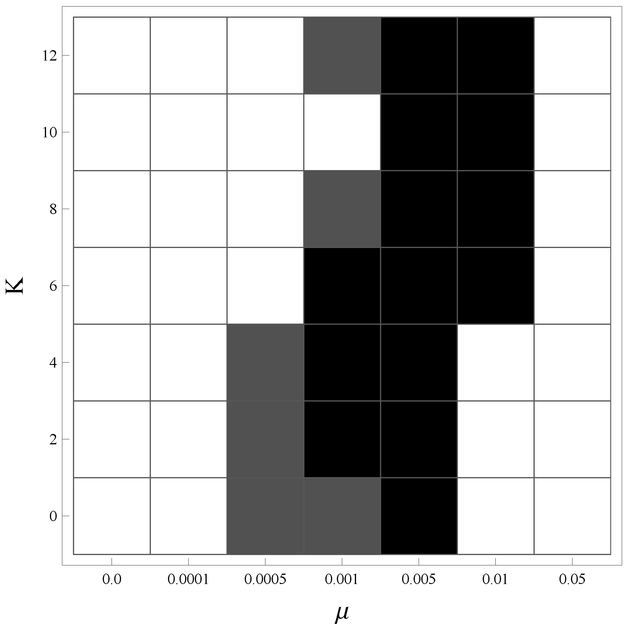
The white (black) cells in the figure show the combinations of K and μ, where an organization with () outperforms the other. The gray cells show the cases where and perform equally well. We performed a two-sample t-test based on PDVs generated by 500 simulations for each set of parameter values. Depending on the results of a variance comparison test, unequal variance or equal variance is assumed in performing a t-test. One organization is said to outperform the other if the mean PDV is significantly greater at a 5% significance level in a one-tailed test.
Interestingly, high-autonomy organizations () tend to perform better when either environment is stable or extremely turbulent, whereas high-conformity organizations tend to exceed the former in mildly turbulent environment. A well-aligned search process based on an assimilated knowledge base in the high-conformity organizations helps the organization to achieve a good balance between search and stability in a changing environment and improve the organizational knowledge increasingly faster than uncoordinated search in the high-autonomy organizations, as we discuss in Section 3.2 (see Figure 3). This mechanism does not work properly when the environment is excessively turbulent, because continuous improvement under assimilated knowledge becomes too slow to chase the “moving carrot.” In such an extreme situation, the value of developing organizational knowledge is low, as it becomes obsolete extremely quickly. In contrast, complexity of tasks does not seem to greatly affect the relative performance of high-conformity organizations versus high-autonomy organizations.
There is a caveat regarding this finding. Note that we are measuring performance with PDVs that put higher weights on earlier periods than on later ones. As seen in the previous section, if we compare the average performance in later periods (or place more weight on the performance in later periods by using a higher discounting factor, δ), a high-conformity organization () outperforms a high-autonomy organization () for a greater range of parameters.
4. Conclusions
This work reveals the possible origin of the tension between exploration and exploitation and identifies the characteristics of the optimal form of organizational learning for a variety of parameter values. We illustrate the important roles played by organizational conformity in facilitating organizational learning. Our results show non-concavity in the optimization problem of organization design and imply that two distinct types of organization can emerge. The high-autonomy organization promotes individual initiatives to experiment with new ideas and building its strength on individual learning. The high-conformity organization, in contrast, assimilates the individual knowledge base and accelerates organizational learning through frequent knowledge sharing among individuals. An organization with a more equal mixture of individual initiative and knowledge assimilation tends to perform worse, especially when the operation is reasonably complex (in other words, interdependency is high enough) and/or the business environment is reasonably turbulent. Although a high-conformity organization tends to be the better choice when the environment is mildly turbulent, a high-autonomy organization tends to be the better choice when the environment is either stable or extremely turbulent.
Another interesting finding is that, when high-autonomy and high-conformity organizations perform equally well in terms of PDV, the former performs better initially, but the latter catches up with and eventually outperforms the former. The difference in dynamics between the two types of organization has implications for the role of structural ambidexterity [22,23,24]. According to this literature, organizations manage trade-offs between conflicting demands by putting in place “dual structures,” so that certain business units focus on exploitation, while others focus on exploration. According to our model, although it is suboptimal to aim for both exploration and exploitation (i.e., to choose the intermediate level of λ) within the same group of people, it might be feasible to have one business unit choose high autonomy and the other choose high conformity. Such an organization may succeed in showing persistently high performance, because the high-autonomy units outperform the high-conformity units initially, but the latter eventually outperform the former if the task is complex or the environment turbulent.
There are two remaining issues to be considered. First, how robust are the results we have illustrated in this paper to changes in the assumptions? Specific rules and processes of updating organizational knowledge in our model would need to be relaxed to see whether our bifurcation results continue to hold under different assumptions. Second, we do not take into account the possibility that the degree of organizational conformity may change as time goes by. This clearly constitutes an important question, particularly, if parameter values, such as the complexity of operation, K, were to change in the course of a firm’s growth. We believe that these issues can be successfully addressed by extending the basic framework we employed in this paper, but leave this to future research.
A. Results from and
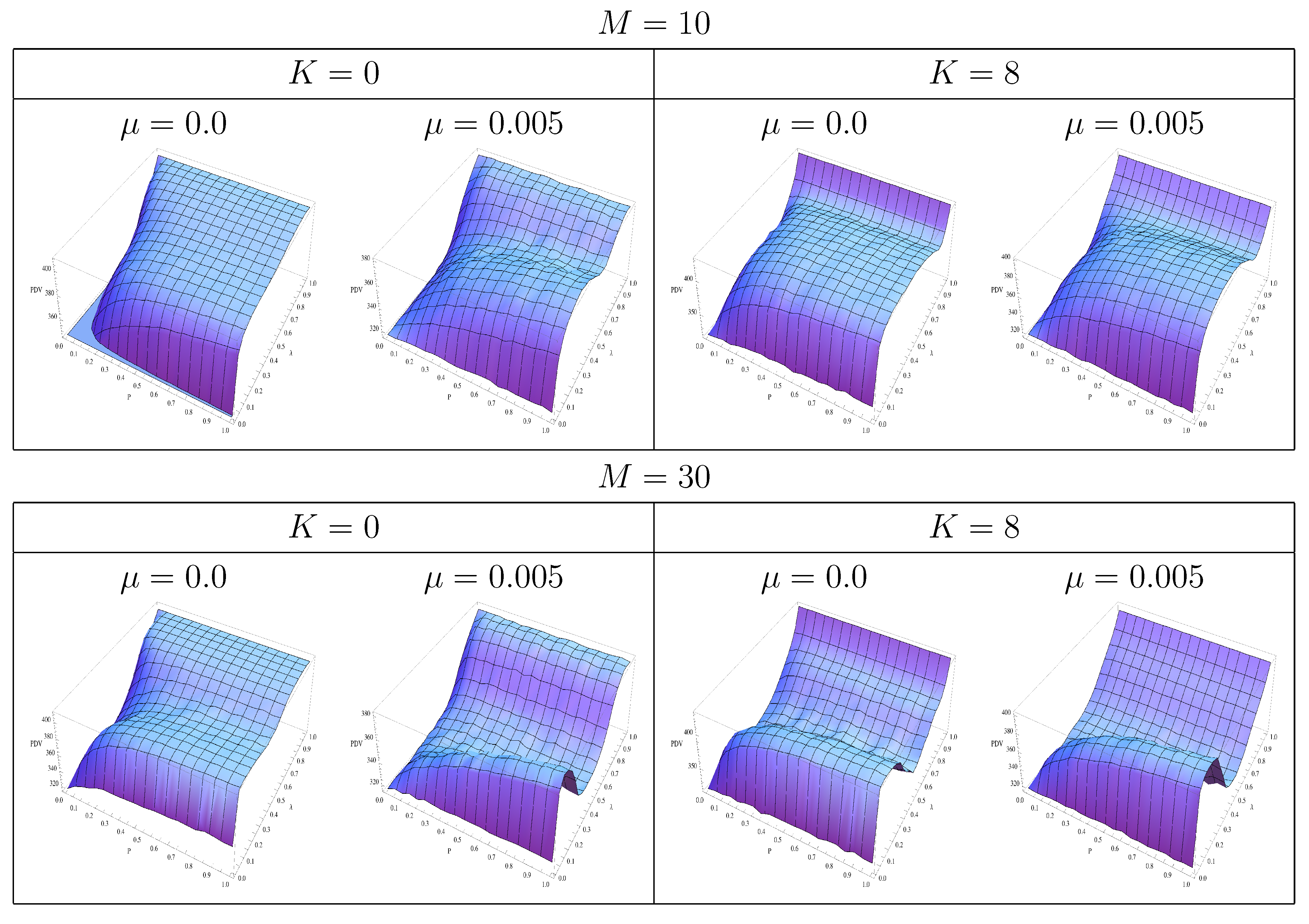
The main text concentrated on discussion of the results for . This appendix presents the simulation results from and , which are qualitatively the same as the results in the main text. Figure 7 shows, in the same format as in Figure 1, PDV with discount factor, (height), for various values of p (horizontal axis) and λ (vertical axis) for four combinations of K and μ. is on the top row and is on the bottom row. As can been seen from comparing Figure 7 and Figure 1, the main results do not change with the changing number of agents in the organization. What does change, is the range of values of that maximizes performance.
Figure 7.
Average PDVs of organizational performances for (top) and (bottom) for four combinations of and . Based on the average results from 100 simulation runs.
Figure 7.
Average PDVs of organizational performances for (top) and (bottom) for four combinations of and . Based on the average results from 100 simulation runs.
Acknowledgments
We are grateful to Tommaso Ciarli and Luigi Marengo, as well as to seminar participants at Hitotsubashi University, participants in the 2009 annual conference of Strategic Management Society, WEHIA 2009, 2009 national conference of the Academic Association for Organizational Science, and the Contract Theory Workshop in Japan for comments and suggestions. This project is partly financed by JSPS-ANR bilateral research grant “BECOA” and JSPS Grant-in-Aid for Scientific Research (B) (No. 21330058).
Conflict of Interest
The authors declare no conflict of interest.
References
- Owan, H. Works Applications, Inc. (A) Aoyama Business School case 2009. November. (in Japanese)
- March, J.G. Exploration and exploitation in organizational learning. Organ. Sci. 1991, 2, 71–87. [Google Scholar] [CrossRef]
- Roberts, D.J. The Modern Firm: Organizational Design for Performance and Growth; Oxford University Press: New York, U.S.A., 2004. [Google Scholar]
- Kauffman, S. The Origins of Order: Self-Organization and Selection in Evolution; Oxford University Press: New York, U.S.A., 1993. [Google Scholar]
- Rivkin, J.W.; Siggelkow, N. Balancing search and stability: Interdependencies among elements of organizational design. Manag. Sci. 2003, 49, 290–311. [Google Scholar] [CrossRef]
- Rivkin, J.W.; Siggelkow, N. Patterned interaction in complex systems: Implications for exploration. Manag. Sci. 2007, 53, 1068–1085. [Google Scholar] [CrossRef]
- Siggelkow, N.; Rivkin, J.W. Speed and Ssearch: Designing organizations for turbulence and complexity. Organ. Sci. 2005, 16, 101–122. [Google Scholar] [CrossRef]
- Siggelkow, N.; Rivkin, J.W. When exploration backfires: Unintended consequences of multi-level organizational search. Acad. Manag. J. 2006, 49, 779–795. [Google Scholar] [CrossRef]
- Barr, J.; Hanaki, N. Organization undertaking complex projects in uncertain environments. J. Econ. Interact. Coord. 2008, 3, 119–135. [Google Scholar] [CrossRef]
- Gavetti, G.; Levinthal, D. Looking forward and looking backward: Cognitive and experimental search. Adm. Sci. Q. 2000, 45, 113–137. [Google Scholar] [CrossRef]
- Marengo, L.; Pasquali, C. How to get what you want when you do not know what you want. A model of incentives, organizational structure and learning. Organ. Sci. 2012, 23, 1298–1310. [Google Scholar] [CrossRef]
- Levinthal, D.A.; March, J.G. The myopia of learning. Strateg. Manag. J. 1993, 14, 95–112. [Google Scholar] [CrossRef]
- Ghemawat, P.; Ricart i Costa, J.E. The organizational tension between static and dynamic efficiency. Strateg. Manag. J. 1993, 14, 59–73. [Google Scholar] [CrossRef]
- Kocher, M.G.; Sutter, M. The decision maker Mmatters: Individual versus group behavior in experimental beauty contest games. Econ. J. 2005, 115, 200–223. [Google Scholar] [CrossRef]
- Cooper, D.J.; Kagel, J.H. Are two heads better than one? Team versus individual play in signaling games. Am. Econ. Rev. 2005, 95, 477–509. [Google Scholar] [CrossRef]
- Bornstein, G.; Kugler, T.; Ziegelmeyer, A. Individual and group decisions in the centipede game: Are groups more “rational” players? J. Exp. Soc. Psychol. 2004, 40, 599–605. [Google Scholar] [CrossRef]
- Krishnan, H.A.; Miller, A.; Judge, W.Q. Diversification and top management team complementarity: Is performance improved by merging similar or dissimilar teams? Strateg. Manag. J. 1999, 18, 361–374. [Google Scholar] [CrossRef]
- Simons, T.; Hope Pelled, L.; Smith, K.A. Making use of difference: Diversity, debate, and decision comprehensiveness in top management teams. Acad. Manag. J. 1999, 42, 662–673. [Google Scholar] [CrossRef]
- Dahlin, K.B.; Weingart, L.R.; Hinds, P.J. Team diversity and information use. Acad. Manag. J. 2005, 48, 1107–1123. [Google Scholar] [CrossRef]
- Reagans, R.; Zuckerman, E.; McEvily, B. How to make the team: Social networks vs. demography as criteria for designing effective teams. Adm. Sci. Q. 2004, 49, 101–133. [Google Scholar]
- Crossan, M.M.; Lane, H.W.; White, R.E. An Organizational Learning Framework: From Intuition to Institution. Acad. Manag. Rev. 1999, 24, 522–537. [Google Scholar]
- Duncan, R.B. The Ambidextrous Organization: Designing Dual Structures for Innovation. In The management of organization; Kilmann, R.H., Pondy, L.R., Slevin, D., Eds.; North-Holland: New York, NY, USA, 1976; Volume 1, pp. 167–188. [Google Scholar]
- Tushman, M.L.; O’Reilly, C.A. Ambidextrous organizations: Managing evolutionary and revolutionary change. Calif. Manag. Rev. 1996, 38, 8–30. [Google Scholar] [CrossRef]
- Gibson, C.B.; Birkinshaw, J. The antecedents, consequences, and mediating role of organizational ambidexterity. Acad. Manag. J. 2004, 47, 209–226. [Google Scholar] [CrossRef]
© 2013 by the authors; licensee MDPI, Basel, Switzerland. This article is an open access article distributed under the terms and conditions of the Creative Commons Attribution license (http://creativecommons.org/licenses/by/3.0/).
Share and Cite
MDPI and ACS Style
Hanaki, N.; Owan, H. Autonomy, Conformity and Organizational Learning. Adm. Sci. 2013, 3, 32-52. https://doi.org/10.3390/admsci3030032
AMA Style
Hanaki N, Owan H. Autonomy, Conformity and Organizational Learning. Administrative Sciences. 2013; 3(3):32-52. https://doi.org/10.3390/admsci3030032
Chicago/Turabian StyleHanaki, Nobuyuki, and Hideo Owan. 2013. "Autonomy, Conformity and Organizational Learning" Administrative Sciences 3, no. 3: 32-52. https://doi.org/10.3390/admsci3030032