Trace Metal Modelling of a Complex River Basin Using the Suite of Models Integrated in the OpenMI Platform


1
Department of Hydrology and Hydraulic Engineering, Vrije Universiteit Brussel, 1050 Ixelles, Belgium
2
Water Resources Research Center, University of Hawaii at Manoa, Honolulu, HI 96822, USA
*
Author to whom correspondence should be addressed.
Environments 2018, 5(4), 48; https://doi.org/10.3390/environments5040048
Submission received: 28 February 2018
/
Revised: 4 April 2018
/
Accepted: 9 April 2018
/
Published: 13 April 2018
(This article belongs to the Special Issue Environmental Toxicology of Trace Metals)
Abstract
:Modelling trace metal dynamics is essential in an integrated modelling framework as trace metals have the potential to be fatal, even when present at low concentrations. Since the degree of bioavailability of a metal depends on its presence in the dissolved phase, it is necessary to keep track of both the dissolved and particulate phase of metals. In general, the well-known partitioning coefficient approach is widely used for trace metal speciation. As such, we applied a parametric approach to relate the partitioning coefficient to several environmental variables. These environmental variables are made available by a suite of physically based models (a hydrologic and diffuse pollution model, Soil and Water Assessment Tool (SWAT); a hydraulic model, Storm Water Management Model (SWMM); a stream temperature model; an in-stream water quality conversion model; and a sediment transport model) integrated using the Open Modelling Interface (OpenMI). For trace metal speciation, two regression techniques, (a) the multi-linear regression (MLR) and (b) the principle component regression (PCR), were used. It is then tested in the Zenne river basin, Belgium, to simulate four trace metals (copper, cadmium, zinc and lead) dynamics. We demonstrated the usefulness of the OpenMI platform to link different model components for integrated trace metal transport modelling of a complex river basin. It was found that the integrated model simulated different metals with ‘satisfactory’ accuracy. The MLR- and PCR-based model results were also comparable. From a management perspective, the river is not heavily polluted except for the level of dissolved zinc. We believe that the availability of such a model will allow for a better understanding of trace metal dynamics, which could be utilized to improve the present condition of the river.
1. Introduction
The European Union (EU) Water Framework Directive (WFD) established in 2000 [1] advocated the requirement of a good ecological status for all surface waters in all member states by 2015. In order to attain this required status, the directive has specified Environmental Quality Standards (EQS) for several priority substances, including trace metals [2]. In response to the WFD’s call for enhancing the status of aquatic ecosystems and reducing pollution from priority substances, large investments were made for the management of the wastewaters draining to the Zenne River, Belgium, resulting in an increase of the quality of the river [3]. Despite these investments, the river still receives high loads of pollutants, especially considering its low discharge. Consequently, the water quality downstream from Brussels does not comply with the requirements set by the WFD. It is in this context that an interuniversity, multidisciplinary research project titled, ‘Good Ecological Status of the river Zenne’ (GESZ), was launched to evaluate the effects of the wastewater management plans on the ecological functioning of the river. It aims to provide advice related to sewage management processes in Brussels through the development of various tools that can compute the evolution of water quantity and quality in the river by measuring multiple variables, including trace metals.
The need for integrated models to gain insight into environmental problems is well appreciated in recent times [4]. Modelling of trace metal dynamics is essential in an integrated framework because some trace metals, such as mercury (Hg), lead (Pb) and cadmium (Cd), have the potential to be fatal even if they are present at low concentrations. This fact is reflected in the WFD, which specifies Cd as a priority hazardous substance and Pb as hazardous substance (Table 1). The WFD requires that these substances be progressively phased out. Note that not all of the trace metals are toxic; some of them are essential as micro-nutrients and are present in high concentrations [5]. Since the degree of bioavailability and thus, the toxicity, of a metal depends on its presence in the dissolved and particulate phases, it is necessary to keep track of both forms of metals in the water column.
The Zenne river basin, Belgium, can be considered a unique and complex river basin. From its upstream predominantly agricultural sub-basins, the river receives mostly the non-point sources pollution. The river is made to exchange water fluxes with a canal at multiple locations to prevent the city of the Brussels from flooding. The proportion of flows from Brussel’s sewer network can be more than 50% of the river’s flow, especially during dry weather flow conditions [3]. Furthermore, the river flow is influenced by the tide of the North Sea at its mouth. Hence, a single model such as the Soil and Water Assessment Tool (SWAT) [10], a hydrologic model, is not suitable as the model cannot simulate either complex interactions of sewer systems or the back water effects of the tide. While hydraulic models such as the Storm Water Management Model (SWMM) [11] can simulate the complex sewer systems and the tidal effect, they are not suited for simulating the non-point sources of pollution. Therefore, in order to have flexibility during the selection of the simulators for the different processes occurring within the basin (i.e., hydrology of the river basin, hydraulics in the river and sewers, erosion and sediment transport, fecal bacteria transport, the fate of trace metals and the carbon-nitrogen-phosphorus cycle), we opted to use the Open Modelling Interface (OpenMI) [12,13]. The OpenMI is an interface which allows for the dynamic linking of different models that are compliant to its pre-established standard. The OpenMI has been successfully and widely applied for the purposes of model integration in such areas as urban hydrology and hydraulics [14,15], sediment transport modeling [16], in-stream water quality modelling [17] and fecal bacteria modelling [18]. Additionally, ample support for using OpenMI has come from multiple different groups and organizations [19,20,21]. Furthermore, there have been growing calls to follow the so-called ‘open source route’ in environmental modelling discipline so as to create a ‘functional collaborative community’ [4,21,22]. As such, use of such platform (the OpenMI) which promotes the use of existing open-source simulators would enhance model re-usability, thereby saving huge amount of time and efforts in developing a new one [23].
In this paper, we used the OpenMI to integrate several physically based models: a hydrological model, the Soil and Water Assessment Tool (SWAT) [10]; a hydraulic model, the Storm Water Management Model (SWMM) [11]; a stream water temperature model; a sediment transport model; and a water quality model. The integrated model would then provide different environmental variables for the newly developed trace metal transport model which then predicts both dissolved and particulate phase of metals using different regression techniques. In order to be able to integrate the models on the OpenMI platform, SWAT and SWMM were migrated to the OpenMI platform, (refer to Shrestha et al. [24] for information on SWMM OpenMI migration). The migration process involved a re-structuring of the engine core of the simulator in such a way that allows it to inherit the running sequences of OpenMI [12]. The other simulators were developed in such a way that they directly became OpenMI compliant. The integrated model was then used to simulate the trace metal dynamics of the Zenne river, Belgium. We believe that with the availability of such an integrated trace metal model, the trace metal dynamics can be better understood and such information could easily be translated into improving the present condition of the river.
2. Material and Methods
2.1. Trace Metal Dynamics in a Riverine System
Trace metals enter the riverine system via two main sources: natural (e.g., weathering, erosion and volcanic actions) and anthropogenic (e.g., domestic and industrial waste water, mining and dredging) [25]. In the river, they are partitioned between the dissolved phase and the particulate phase. Some major processes of metal partitioning are adsorption-desorption, complexation-decomplexation, precipitation-dissolution and biological uptake-organic matter degradation [26,27,28,29]. Since the degree of bioavailability and thus, the toxicity, of a metal depends on its presence in the dissolved and particulate phases, it is necessary to keep track of both forms of metals in the water column. It should also be noted that the bed sediments constitute a reservoir for dissolved trace metals [30,31,32].
As per current modelling practices, the use of metal partitioning coefficients—also known as distribution coefficients—to partition the metals between the dissolved and the particulate form is widespread [33]. The partitioning coefficient (Kd in L/kg) is defined as the ratio of the particulate metal concentration (MeP in μg/kg of sorbed material) to the dissolved metal concentration (MeD in μg/L of water). In most cases, Kd is considered a constant. However, there is growing realization that Kd varies in accordance with changes in environmental variables, such as pH and dissolved oxygen (DO) [34,35].
Different techniques that may be used to simulate Kd are: (a) parametric models; (b) isotherm adsorption models and (c) mechanistic adsorption models [36]. A parametric model describes the variation of the distribution coefficient through empirically-derived relationships between Kd and sediment and water quality variables. Such models are applicable only within the range of the values of the variables used to derive the empirical relationship. Furthermore, owing to the statistical nature of the equations, they do not provide an explanation of how metals associate with particulate matter [36]. An adsorption isotherm model describes the association of the metals with the solids for constant values of variables such as pH and temperature [37]. This kind of model provides information on the adsorption mechanism of the metals. The particulate metal concentration is evaluated based on the dissolved metal concentration and constant parameters. This simplifies the dependence of the metal concentration on variables such as organic matter [36]. Isotherm models are available in a variety of forms, including the Languir model [38], the Freundlich model [39] and the Dubinin-Radushkevich equation [40]. A mechanistic model takes into account the dependency of the distribution coefficient on a number of variables such as the metal concentrations, the concentrations of competing ions and the surface charge of the adsorbent [36]. Although these models may be expected to provide better results than the parametric models or the isotherm models [41], they are complex and require a large number of input variables [36].
Once a trace metal is separated into the dissolved and the particulate forms, it needs to be routed. In general, its fate is governed by a 3-D advective-diffusion equation [42]. However, several simplifications of the equation exist for various situations. For example, for a river that is long enough when compared to the distance of complete mixing over the entire x-section, a 1-D approach is appropriate [43]. A further simplification for a situation in which a river is divided into several river segments and within which perfect mixing is assumed, the 1-D equation further reduces to an ordinary differential equation which is commonly known as the completely stirred tank reactor (CSTR).
2.2. The Study Area
The Zenne River is a part of the international Scheldt basin. It drains an area of 1162 km2 and runs through the three administrative regions of Belgium: the Walloon Region (574 km2), the Brussels Capital Region (162 km2) and the Flemish Region (426 km2). After a length of approximately 100 km, it meets with the Dijle River, where it is subject to the tidal influence of the Scheldt River. The river basin is crossed by the Brussels-Charleroi canal and the Brussels-Scheldt Sea Canal. In the Walloon Region, the canal is fed by former tributaries of the river (Figure 1).
In the area between the borders of the Walloon and the Brussels Region, different tributaries discharge into the river. The canal also receives water from the river through several overflow structures in order to prevent flooding in the Brussels region. Excess water in the canal can be discharged back into the river downstream from Brussels. The basin has a population density of about 1260 inhabitants/km2, which makes it the most densely populated basin of the Scheldt basin [44]. The land-use in the catchment is dominated by agriculture (51%), primarily in the upstream part of the basin and by urban regions (19%) in the downstream section. There are several waste water treatment plants (WWTPs) in the basin. In the Brussels area, the river receives the sewage waters from the WWTP Brussels South (360,000 inhabitant-equivalents, in operation since 2000) and the WWTP Brussels North (1,000,000 inhabitant-equivalents, in operation since 2007).
The Zenne River is also a fine example of how a river system’s ecological and hydrologic continuum can be modified by anthropogenic pressures. The prosperous textile craft industry at the beginning of 11th century along the banks of the Zenne River led to a significant population increase. As a result of industrialization and associated urbanization and sanitation needs of the inhabitants living in the catchment, the river had already been heavily polluted [45,46]. The drawn discharge from the Zenne to feed a canal which ran parallel to the river also contributed to worsening of the situation [47]. Thus, the river was required to be covered for sanitation purposes. Once the river was covered, water quality preservation was no longer a priority for Brussels’ authorities [3] until the introduction of enforcements imposed by the Urban Waste Water Treatment Directive (UWWT) [48] in 1991.
2.3. The Trace Metal Simulator
As stated in Section 2.1, there exists different techniques to simulate the partitioning coefficient (Kd). We opted for a parametric model because various input data required for other techniques (e.g., isotherm adsorption models and mechanistic adsorption) were not available. The parametric model for Kd was based on readily available (monitored) or computable environmental variables. As we intended to use the trace metal model as a component model in an integrated modelling chain, a simple yet robust model was needed to limit the computation time which is considered to be a severe bottleneck of an integrated model.
In this study, we applied two regression techniques: a multilinear regression (MLR) and a principal component regression (PCR). In an MLR, the dependent variables are determined directly from the independent variables while in a PCR, new components are defined to be used as the independent variables. For both the MLR and the PCR, we first determined an empirical relationship for the calculation of Kd based on physicochemical variables and total metal concentrations (MeT). The considered physicochemical variables were: electrical conductivity (EC), dissolved oxygen concentration (DO), the pH, the suspended particulate matter (SPM) concentration and the temperature (Ts). Interaction terms were introduced and selected based on the assessment of the variance inflation factor (VIF) [49]. For an MLR, interaction terms with excessive multi-collinearity (VIF > 10,000) were eliminated. This retained the terms with smaller VIF values which indicated lessened multi-collinearity. Additionally, the Bayesian information criterion (BIC) [50] was used to determine the model parameters that provided a good compromise between goodness of fit (R2) and predictive power reflected by the predicted residual sums of squares (PRESS) statistic [51]. The model with the lowest BIC was selected as the final model.
It should be noted that we transformed all of the variables before they were subjected to regression using a Box-Cox (BC) transformation [52] to ensure a normal distribution of the variables. The parameter (λ-value) of the BC-transformation was subjected to calibration. We found the parameters to be −0.208, −0.403, −0.065 and −0.204, respectively, for MeT-Cu, MeT-Cd, MeT-Pb and MeT-Zn. Similarly, λ-values of 2.057, 1.101, 0.396, −0.632 and −0.359 were found for Ts, pH, DO, EC and SPM, respectively. The assumption of normality was checked using the Shapiro–Wilk test [53].
Once a function for the partitioning coefficient, Kd (L/kg), is defined, MeD (μg/L) and MeP (μg/g) can be derived from the total metal concentration, MeT (μg/L) and the suspended particulate matter, SPM (mg/L), concentration as:
Furthermore, we adopted the principles of CSTR to route the metal species. The metal species were considered not to undergo any conversion process within the time frame of relevance.
An accurate information of water fluxes was required in order to route the metal constituents. Owing to the nature and complexity of the river basin under consideration, we selected the SWAT model for the simulation of the river basin processes from the predominantly rural sub-catchments in the upstream part of the river basin. SWAT is a physically-based, semi-distributed, hydrologic simulator and one of the most widely used models to simulate the basin processes [10]. The SWAT, being a hydrological model, cannot simulate complex hydraulic processes such as back water effects, nor two way interactions between, for instance, a sewer system and a river. We used a hydraulic simulator, the SWMM, for the downstream reach of the river to address all of the different components of the system (e.g., the sewer systems with their auxiliary structures, the canal and the river in tidal reach). The SWMM is, primarily, a dynamic rainfall runoff simulator for computing the runoff quantity and quality from urban areas [11]. The SWAT-SWMM combination was therefore deemed necessary to simulate water fluxes for a complex basin such as the Zenne.
An additional simulator needed to be developed for the sediment as we intended to have a trace metal model which would track both dissolved and particulate forms (see Equations (1) and (2)) using the partitioning coefficient. The sediment transport simulator we developed is based on Shield’s approach for the initiation of motion based on critical shear stress and critical particle diameter in conjunction with Velikanov’s energy equation for the limitation of the carrying capacity. A thorough description of the simulator is presented in Shrestha et al. [54].
Since the partitioning coefficient depends on various physiochemical variables, a separate simulator for the water quality conversion processes needed to be developed. We used river water quality model No. 1 (RWQM1) principles for the water quality conversion processes. A thorough description of the simulator is presented in Shrestha et al. [17].
Additionally, since many kinematics of the sediment transport simulator and the water quality simulator depended on the stream water temperature, a temperature simulator also needed to be developed. The temperature simulator we developed is based on a non-linear regression fit between the air and the stream water temperatures, as suggested by Mohseni et al. [55]. Further information of the simulator can be found in Shrestha et al. [56]. Finally, a trace metal transport simulator, described in more detail in following sections, was developed to simulate trace metal dynamics and speciation.
2.4. Model Inputs, Build up, Calibration and Validation
Table 2 provides an overview of the types of data that were used for the build-up, the calibration and the validation of the developed models. The following paragraphs elaborate the issues for each model component. Emphasis is placed on the inputs, build-up, calibration and validation of the trace metal component.
The SWAT model is the first model of the integrated modelling chain. Hence, it is built up, calibrated and validated on a standalone basis. The data sources and the data resolutions used for the model are presented in Table 2. We used the years 1998–2008 for calibration and the years 1988-1997 for validation, using daily stream flows recorded at Tubize (Figure 1). We optimized the related parameters (see Leta et al. [15] and Leta et al. [57] for details). For sediment and water quality simulations, we used the years 1998–2008 for calibration and the years 1994–1997 for validation. For the calibration of the sediment module, we used sediment concentrations measured at Quenast (Figure 1). Five water quality variables (DO, BOD, NH4, NO3 and DIS-P) measured at Quenast were used for a manual calibration of the water quality-related parameters.
A SWMM model was built for the section of river between the border of the Walloon—Flemish region and for the mouth of the river (Figure 1). The canal network, including the exchange points with the river, was also modelled using SWMM. The SWMM model included simplified representations of the sewer systems that are connected to the major WWTPs (Figure 1). As SWMM requires rural catchment runoff as a boundary condition and the runoffs were simulated using the SWAT model, an OpenMI-integrated SWAT/SWMM model was implemented. The integrated model was calibrated and validated using hourly stream flows observed at three locations along the river—Lot, Vilvoorde and Eppegem (Figure 1). We used the stream flow data from 2007 to 2008 to calibrate the model and flow data from 2009 to 2010 for the validation.
As the next step, we added the temperature model to the SWAT-SWMM integrated model. We used stream water temperature data at three locations along the river, Lot, Vilvoorde and Eppegem (Figure 1) from the years 2007 to 2010, as recorded by the VMM, to validate the model.
Next, the sediment model was added. The quantities of flow and sediment exchanged at different element sets such as links, nodes and sub-basin outlets are shown in Figure 2. Imposed boundary conditions for the integrated model are also shown in Table 2. We calibrated the parameters (see Shrestha et al. [58] for details) of the model using sediment concentrations for Lot, Vilvoorde and Eppegem from 2007 to 2008. The integrated model was validated using sediment concentrations from 2009 to 2010.
For the water quality model, SWAT-SWMM-Temperature-Water Quality components were integrated in OpenMI. Figure 2 shows the data exchange between the different model components that were used for the simulation of the water quality. Imposed boundary conditions for the model are presented in Table 2. The parameters of the water quality model (see Shrestha et al. [17] for details) were determined heuristically, based on measured water quality variables during dry weather flow (DWF) conditions. The model was then validated based on long term simulations, using monthly water quality concentrations measured by the VMM at Lot, Vilvoorde and Eppegem (Figure 1).
Finally, an integrated trace metal transport model was implemented which consisted of six model components (Figure 2). We considered of metals: copper (Cu), cadmium (Cd), zinc (Zn) and lead (Pb). According to the WFD, Cd is considered to be a ‘priority hazardous substance’ and Pb is considered a ‘priority substance’.
In this model build up, we used data gathered from the GESZ campaigns. It included longitudinal profiles of various physicochemical variables and MeT concentrations measured during dry weather conditions in different seasons (five campaigns). In addition, two campaigns were organized to gain information about the water quality during storm conditions, including a 24-h campaign. In order to calibrate and validate the derived relationship, we divided the data into two groups. ‘Group-1’ (Table 3) consisted of 113 samples taken from four DWF campaigns and one 24-h set of continuous measurements. This group made up the calibration data set. ‘Group-2’ consisted of 39 samples taken from one DWF campaign, one rain campaign and 10 randomly selected datasets from ‘Group-1’ in order to obtain wider variability in the data set. ‘Group-2’ was used for validation purposes. The decision to select two sampling campaigns for ‘Group-2’ was made in consideration of the fact that these measurements showed clustering, as shown in the score plot (Figure S1) where four components F1 to F4, describing 83% of the total information from the data, are plotted. A score plot shows a map of these observations. Data points close to the origin display average properties of the data while data grouped together or in a quadrant could indicate data anomalies. Similarly, outliers could be detected too. As can be seen on both plots (Figure S1), the data corresponding to sampling campaign of December 2009 fall in the third quadrant for both plots. Similarly, a clear cluster corresponding to data of June 2011, a wet weather campaign, is especially visible in Figure S1a.
In addition to the rural catchment MeT inputs which were estimated with the derived regression equations, we used constant MeT concentrations at WWTP outlets, at CSO sources and at the outlet of the river based on the GESZ measurements. Figure 3 shows the GESZ measurements of total metal concentration at the outlets of WWTP and at GESZ station Z13, located near the river outlet. Hence, mean observed MeT concentrations were imposed at the river outlet during the sampling campaigns. Although there exists variation among the total metal concentrations, we had to impose an average constant concentration due to a lack of an observed time series. Although we are aware that more accurate boundary conditions needed to be imposed at locations such as the WWTP outlets, the CSO outlets and the river outlets, we did not have another viable option.
The integrated trace metal model was validated using MeT and MeD concentrations measured by the VMM measurements at three stations: Lot, Vilvoorde and Eppegem (Figure 1). Particulate metal (MeP) concentrations of metals were not available for the considered data period of 2007–2010. Moreover, several measurements of total and dissolved trace metal concentrations were below the detection limit and, therefore, had to be eliminated from the dataset.
2.5. Performance Evaluation of the Model
To evaluate the accuracy of model results, we used the percentage bias (PBIAS), the ratio of the root mean square error to the standard deviation of the measured data (RSR) and the Nash-Sutcliffe efficiency (NSE) [59]. The main reason for using these statistics was to assign a qualitative rating to the model results. We used the ranges for these goodness-of-fit statistics as proposed by Moriasi et al. [60] to determine a qualitative assessment of the model (i.e., very good, good, satisfactory, or unsatisfactory) for each of these indicators. A global qualitative assessment of the model was made by assigning a score of 4 to a very good model and assigning a score of 1 to an unsatisfactory model for each of the criteria and then calculating the average score for the three criteria. The widely-used root-mean squared error (RMSE) and mean absolute error (MAE) were used to complement the aforementioned dimensionless goodness-of-fit statistics.
3. Results and Discussion
For clarity purposes, detailed results of each model component are not presented here. Rather, a qualitative assessment of the different components is provided. For the optimized stream flow related parameters of the SWAT model, we refer toLeta et al. Optimized flow-related parameters for one of the collectors of the sewer systems of Brussels—the Paruck collector—can be found in Nkaika et al. [60]. Similarly, water quality parameters of the SWAT model and parameters of the integrated water quality model can be found in Shrestha et al. [17]. Optimized parameters of the sediment transport and temperature models can be found in Shrestha et al. [54]. The following paragraphs, therefore, focus on the detailed results of the trace metal model.
3.1. The Total Metal Concentrations at The Outlets of Rural Catchment
Table 4 provides an overview of the regression equations for the different metals. In the case of the MLR, the use of EC, pH and SPM as predictors in various combinations resulted in the lowest BIC for the MeT-Cd (Figure S2). For MeT-Cu, two variables (EC and SPM) were the best set of predictors. For MeT-Pb, four variables (EC, SPM, Ts and pH) were selected. For MeT-Zn, three variables (EC, pH and SPM) were the best set that could be determined. DO did not appear in the set of predictors for any of the metals. EC and SPM influenced the MeT concentrations the most negatively and positively, respectively. The results were expected as the loading plot (Figure S3) showed that MeT and SPM lie on the same quadrant, while MeT and EC do not. Indeed, a loading plot showed relationships amongst the variables that were taken into consideration. Variables close to one another exhibit high correlation while those on the opposite side of the origin exhibit negative correlations. Moreover, similar samples are placed together. Hence, distance from the origin to the variable and its quadrant location carries special meaning.
The quality of the regression models varies from ‘Unsatisfactory’ to ‘Very Good,’ depending on the considered metal, the analysis technique used and the dataset (Table S3). A graphical representation of the results is shown in Figure 4a. In the figure, most of the data points fall inside the +/−1-standard deviation line (i.e., within 68% of the confidence interval) of the predicted value. For all cases, the predicted MeT were underestimated for higher MeT observations. We found that these higher MeT observations corresponded to one specific sampling campaign, the 24-h campaign (Group-1, Table 3) and at one specific location, Z4. It should be noted that the SPM appeared in the regression equations for all MeT (Table 4) and influenced the MeT predictions positively (i.e., higher SPM resulted in higher MeT—see the regression equation in Table 4). We found that the measured SPM in that particular sampling campaign and at that particular location was lower (29 ± 7 mg/L) than the DWF average value (43 ± 35 mg/L). The underestimation could, thus, be related to this.
Globally, it may be concluded that the results of both analysis techniques are comparable. From the statistical indicators and graphical plots, it can be derived that the PCR technique performed slightly better for Cd and Zn, while MLR performed better for Pb. However, a general trend that can be derived from Table 4 is that the PCR fared better during the calibration period (i.e., had higher R2 values) than did the MLR. On the other hand, the predictive capability of PCR was generally lower than the MLR’s as indicated by higher PRESS statistics. Hence, when the derived relationships were subjected to a different range of independent variables, the multi-linear regression (MLR) was expected to fare better than the PCR.
3.2. The Distribution Coefficients
In the loading plot (Figure S3), the EC and the Log Kd are lying in opposite quadrants, meaning that the EC has a negative influence on the LogKd. The regression equations (Table 4) confirm this, especially for Log Kd-Cd and Log Kd-Zn. The quality of the regression models ranged from ‘Satisfactory’ to ‘Very Good’ (Table S3). Figure 4b shows predicted and observed Log Kd data sets. The performances of the MLR and PCR derived Log Kd equations are fairly comparable. For most cases, however, it appears that the PCR-based regressions provided somewhat better fits, as indicated by higher values of R2, lower values of PRESS (Table 4) and higher performance ratings (Table S3). However, the goodness-of-fit statistics for Log Kd-Zn show that, for both the MLR and the PCR analysis, the correlation was significantly lower than that for the other metals. While the average tendency was represented fairly well (PBIAS < 4%), the values of RSR and NSE, indeed, pointed to a lower accuracy. The NSE was below zero for the PCR derived Log Kd-Zn, even for the calibration period. The negative values for NSE and the higher values for RSR during the validation period indicate that the regression equations for all of the Log Kd performed poorly when subjected to different conditions than those used for the calibration.
3.3. The Results of the Integrated Trace Metal Model
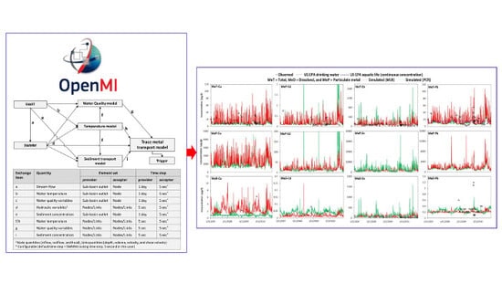
As already indicated, the predicted metal concentrations are validated using observed concentrations at three stations: Lot, Vilvoorde and Eppegem. For clarity purposes, we present simulated and observed total, dissolved and particulate metal concentrations at the most downstream stations—Eppegem (Figure 5). Table 5 shows the goodness-of-fit statistics of the simulated results. It should hereby be noted that the quality of the particulate metal concentrations simulations could not be evaluated as the latter concentrations were not measured.
As evident in Figure 5, at Eppegem, the PCR-based results matched the observed total copper levels well, while the MLR-based simulations were systematically higher than the PCR-based simulations. On average, the bias for the MLR simulations was ca. 12%, compared to ca. 4% for the PCR simulations (Table 5). The error statistics (MAE and RMSE) also pointed to a slightly better quality of PCR simulation. On average, the goodness-of-fit statistics pointed to a ‘Satisfactory’ quality of both model results. For the distribution coefficients, the PCR-based values were systematically higher than the MLR-based simulations. Accordingly, the MLR-based dissolved Cu levels were higher compared to the PCR simulations. For the dissolved Cu, the PCR-based results matched the (2) observations best. The number of observations was, however, too low to draw straightforward conclusions on this issue. Both models produced comparable results for particulate Cu.
For total cadmium, both models showed comparable results. However, this was not the case for the distribution coefficient. The PCR simulations showed a higher variability (4.9–7.4; average 5.5) compared to the MLR simulations (5.9–6.8; average 6.1). The average and the variability of the PCR simulations was comparable to that of the GESZ measurements (4.3–7.1; average 5.5). In this regard, we can consider the PCR predictions better than the MLR predictions. The overestimation of the MLR-based distribution coefficient could be related to the overestimation of dissolved oxygen by the model for Eppegem (PBIAS ≈ 42%—Table 5), as the dissolved oxygen was positively correlated to the distribution coefficient for Cd (Table 4). Better prediction of the PCR simulations was also reflected in the dissolved Cd simulations (Figure 5), where the PCR simulations captured the two observations while the MLR simulations underestimated them. As expected, the MLR-based particulate Cd concentrations were slightly higher than the PCR-based concentrations.
The total zinc concentrations simulated by both models were fairly comparable (Figure 5). While the goodness-of-fit statistics pointed to the same overall quality (‘Satisfactory’) of the model results, the MLR-based results had slightly lower PBIAS and better RSR and NSE values. As was also evident in the plot, both models significantly overestimated the low Zn concentrations. As was also the case for Lot and Vilvoorde, the distribution coefficients simulated by both models were different. The MLR-based simulation showed a quasi-constant distribution coefficient (4.3–4.8; average 4.4), which was in contrast to the higher variability and average that was observed during the GESZ campaigns (4.0–7.4; average 4.9). The PCR-based simulation showed a higher variability (1.5–5.16; average 4.3). However, the average was too low when compared to the GESZ measurements. This rather poor quality of the models was somehow expected, as both the MLR-based and the PCR-based regression equations showed low R2 values, high PRESS values (Table 4) and a poor overall quality (Satisfactory; Table S3) compared to other metal. As for the total Zn concentration, the dissolved Zn concentration was overestimated by both models. On average, the overestimation from the PCR-based model (PBIAS ≈ 33%) was higher than that from the MLR-based model (PBIAS ≈ 30%). A slightly better performance of the MLR-based model was evident in the MAE and the RMSE.
Both of the models tended to represent the trend of the total Pb observations fairly well (Figure 5). On average, the PCR-based simulations showed a lower bias (ca. 3%) and lower error statistics (MAE and RMSE values of ca. 14 and 19 µg/L, respectively) than the MLR-based simulations (PBIAS = 9%, MAE = 16 µg/L and RMSE = 20 µg/L). The goodness-of-fit statistics pointed to a ‘Satisfactory’ quality of the results for both models. The distribution coefficient results showed that the MLR-based simulations (average: 6.9) were comparable to the PCR simulations (average: 6.8). For the dissolved Pb, the goodness-of-fit statistics pointed to an ‘Unsatisfactory’ quality of both models, whereby the MLR-based results were slightly better than the MLR-based results (Table 5).
Unlike the situation at Lot where rural catchment runoff dominates, the metal dynamics at Vilvoorde, located just outside Brussels, were dominated by WWTP effluents and the sporadic CSO events because the Brussels region added higher water volume than what was entered into it (Table S1). In Brussels, the main pollution sources were the WWTPs discharge and the CSO, occurring during wet events. Hence, the inability of the integrated model to simulate the trace metal dynamics at Vilvoorde with high accuracy (Table 5) was not only due to the propagation of the errors observed at Lot but also due to assumptions inherent in imposed concentrations at the WWTPs effluent and the CSO outlets. Especially given that the streamflows at Vilvoorde (Table 5) were simulated with ‘Very Good’ and ‘Good’ accuracy, this rules out the possibility of over-and under-dilution effects. The only major pollution source located after Vilvoorde was the Woluwe CSO outlet. The WWTP effluent of a small plant at Grimbergen was another pollution source. As with Vilvoorde, the inaccuracy of an integrated model to represent the metal dynamics with high accuracy was due to the propagation of model errors and to the underlying simplifications on the imposed boundary condition at the WWTP effluent and the CSO outlet.
3.4. Ecological Status of River Zenne Based on Long Term Simulation Results
The ecological status of the Zenne can be categorized by comparing the long-term (2007–2010) simulation of total, dissolved and particulate metal concentrations against the mandatory levels of different legislations (Table 1). To do so, the simulated instantaneous concentrations were compared against US EPA drinking water quality standard [7] and against the US EPA aquatic life standard [8]. Similarly, the annual average concentrations were calculated to compare these against the Flemish standard [9], the EU ecological quality standard [2] and the EU standard for the quality of fresh waters to support fish life [10].
At Lot, only the dissolved Cadmium levels exceeded the US EPA drinking water quality standard. However, the frequency was very rare. In fact, the level was crossed only three times over the entire time span of 2007–2010. Similarly, the dissolved Zinc crossed the US EPA aquatic life standard only in the summer season in the PCR-based simulation. Moreover, the annual average of dissolved Zinc concentration has, on average, crossed the Flemish basic quality standard (Table 6).
Despite Vilvoorde’s location downstream of major pollution sources (e.g., effluents of major WWTPs and combined sewer flows during wet weather), the situation was not exceptionally alarming. In fact, the ecological status of the river was comparable to that of Lot. However, the levels of dissolved Zinc were almost three times that of the levels at Lot. Hence, the instantaneous concentrations have frequently crossed the US EPA aquatic life standard for all seasons and the annual average concentrations were consistently higher (3.3 times on average compared to Lot concentrations) than the Flemish basic quality standard (Table 6).
At Eppegem, the level of dissolved cadmium has, indeed, was higher by 3.5 times, on average, compared with concentrations at Lot and 1.5 times, on average, when compared with concentrations at Vilvoorde. However, it has seldom crossed the US EPA aquatic life criteria standard (Figure 5). Similarly, the dissolved Zinc concentrations continued to increase, crossing the US EPA aquatic life criteria standard for almost the entirety of the time (Figure 5). The annual average concentrations were always higher than the Flemish basic quality standard. In fact, the dissolved Zinc concentrations at Eppegem increased by 1.5 fold and 3.5 fold when compared with concentrations at Vilvoorde and Lot, respectively (Table 6).
Overall, the ecological status of the Zenne River was good across all reaches of the river, except for the dissolved instantaneous Zinc concentrations which tended to cross the US EPA aquatic life standard. The annual average concentrations also tended to be higher than the Flemish basic quality standard.
3.5. Limitations of the Study
Models used to represent complex and interrelated environmental systems are always a simplification of reality. The level of simplification depends on the intended use of the model and availability of data to build-up, calibrate and validate the model, as well as on external resources (e.g., time and money). While we tried to represent this complex river system using a combination of different existing models (e.g., SWAT and SWMM) and new models (temperature, sediment transport, water quality conversion and trace metal), there were some underlying simplifications that needed some clarification. Most of these assumptions were forced due to data limitations. Furthermore, those who are involved in environmental modeling, are aware of the difficulty of acquiring high quality data of water quality variables, especially metal species. Generally, most of the data are collected to fulfill certain specific goals like we did in the scope of the GESZ project (refer to Table 3 for the sampling campaigns conducted in the scope of the project). Moreover, data for some extreme events, such as the CSOs, are normally difficult to monitor unless an automatic sampler is installed or a dedicated crew is available on a stand-by basis [61].
The major limitations of this work were the assumptions made on the imposed boundary conditions at important pollution sources (e.g., at WWTPs, CSO and the river outlet) which were kept constant in our current implementation and were obvious simplifications of reality. To our knowledge, the management organizations of the Brussels’ sewer systems and thus, the WWTPs, have no plan to monitor trace metal dynamics for either of the WWTPs effluents or for the CSOs any time soon.
As the WWTPs inside Brussels were especially large and the influents during the dry weather conditions were quite constant, larger variations during storm conditions were dampened due to higher residence time (order of magnitude was about a week). At CSO sources, the variations in an urban drainage system such as the one in Brussels, will of course be large as have been observed by various researchers such as Lee et al. [62]. The peak concentration of a particular pollutant will depend on factors such as the spatial extent of the system, the complexity of the drainage network, rainfall intensity and antecedent dry days. Hence, researchers have traditionally made use of the Event Mean Concentration (EMC) [63]. Since the trace metal concentrations during CSO events were determined based on instantaneous measurements, a true EMC could not be calculated. While we are aware of the importance of CSO events as short-term intense pollution sources, it is evident, in our case, that the CSO’s volumetric contribution in an annual scale was not significant (Table S1 and Figure S5). To further investigate this issue, we arbitrarily increased the metal concentrations at the CSO outlets by 20% and 50% relative to currently imposed concentrations and found that the trace metal concentrations at a downstream station (Eppegem) would increase by, on average, 5% and 12%, respectively. Had we missed the CSO concentration by 50%, the effect would still have been within the measurement errors of most water quality variables (~15%, Table S2). Furthermore, the governing legislations such as the Flemish (VLAREM, 2010) and the EU (EU, 2006; EU, 2008) impose annual averaged limits to the trace metal concentrations in the Zenne River. Finally, the constant metal concentrations imposed at the river outlet (Figure 3) only affected the river up to 9 km upstream from the outlet. Indeed, hydraulic simulation results showed backwater effects up to that distance (Figure S6). For an accurate boundary condition at the river outlet, a 2-D model of the Dijle River (the outlet of the river Zenne) would have needed to have been extended to the Scheldt estuary and coupled with our integrated model, which was not within the scope of this work.
Furthermore, we did not conduct a thorough evaluation on the suitability of different integrated modelling platforms, which is one of the limitations of this work. It should be noted that integrated modelling platforms such as The Invisible Modelling Framework (TIME) [64], Framework for Risk Assessment Analysis of Multimedia Environmental System (FRAMES) [65], The object Modelling System (OMS) [66] and so forth, are widely used for model integration. Our choice of the OpenMI as model integration platform was slightly influenced by its growing popularity in Europe and many projects in the region such as SEAMLESS [67], OpenMI-Life [68], SENSOR [69], NITROEUROPE [70], EFORWOOD [71] and so forth, used the OpenMI to integrated different legacy and new models.
Moreover, it should be noted that the EU WFD [1] explicitly specifies ‘quality elements for the classification of the ecological status’ as: (a) biological elements (composition and abundance of aquatic flora and fauna), (b) hydro-morphological elements supporting the biological elements (hydrological regime, river continuity and morphological conditions) and (c) chemical and physicochemical elements supporting the biological elements (thermal, oxygen, nutrient, acidification and salinity conditions) of waterbodies. The directive also specifies a list of priority substances which needs to be systematically phased out. It is thus clear that the directive gives biological analyses precedence over chemical ones. To this end, it can be argued that bioavailability of trace metals should have been validated by analyzing multiple sentinel organisms as various processes and factors affect the bioavailability of different trace metals to different organisms [72,73,74,75,76,77,78]. This is another limitation of this work.
3.6. Usefulness of the OpenMI Platform for Integrated Modelling of a Complex River Basin
In light of the growing realization over the need for an integrated approach to holistic water management of river basins [4,22], it was demonstrated that use of loosely coupled, component-based, ‘standard’ environmental modelling framework—the OpenMI is feasible in such a complex river basin. Moreover, there is a need of promoting, practicing and sharing ‘open source’ developments among the practitioners [21] and OpenMI standard interface is nicely tailored for such purposes. Use of such ‘standard’ would inevitably need some extra effort to conform the design of the (standard’s) engine interface. It can be stated that even for a user which is not a software specialist (but has some level of knowledge and experience in programming), there is quite a substantial support in terms of documentations, demonstrations and training materials in assisting for the development of OpenMI-compliant components [21]. The main benefits of the OpenMI, as the author believes, are that it allows reusability of legacy models which are the results of substantial investment of time and money and it is an ‘open standard’ thereby allowing to share developments with wider user communities. While concerns have been raised regarding the OpenMI based data-exchange induced computation time overhead (e.g., Buahin & Horsburgh [79]), in our case, we reported in Shrestha et al. [54] that the overheard related to the run-time communication was found not to be significant (just 14% increased due to OpenMI based data exchange). However, with the advancement in computing technology, one can adopt parallel computing, grid computing and so forth, to overcome the slightest overload on computational time. On the other hand, another big advantage of OpenMI, as we see it, is that it allows to check the accuracy of each component of an integrated model and to more easily locate the possible sources of errors in the model. For instance, in this integrated trace metal model, the accuracy of simulation results of SWAT, SWMM and temperature model components (and their combinations, links ‘a’ to ‘f,’ Figure 2) is, in general, either ‘Good’ or ‘Very Good’ (Table 5). The accuracy of model simulations tends to deteriorate for the sediment transport and water quality model components (Table 5). As the trace metal model component requires input of different environmental variables (links ‘g’ and ‘i’, Figure 2) from the sediment transport and water quality model components, the ‘satisfactory’ accuracy of the trace metal model can thus also be attributed to the results of these components, in addition to the trace metal model component itself. Hence, in order to improve the accuracy of the trace metal model simulations of the integrated model, besides overcoming all the limitations as stated in Section 3.5, one can focus on improving the robustness (hence the accuracy) of the sediment transport and water quality components or one can simply replace these components in a ‘pick and plug’ manner with a more robust component. This flexibility as offered by the OpenMI platform, we believe, is very important and significant in the field of environmental modelling.
4. Conclusions
In this paper, we demonstrated the usefulness of the OpenMI platform to link different model components for integrated trace metal transport modelling. This approach is innovative in the sense that the different model components run in parallel over the entire river system. We found such a manner of model integration to be very useful to represent a complex river system such as the Zenne River in Belgium. The integrated model consisted of a hydrologic and diffuse pollution model (SWAT), a hydraulic model (SWMM), a stream temperature model, an in-stream water quality conversion model, a sediment transport model and a trace metal transport model. For this, the existing simulators, SWAT and SWMM, were migrated into the OpenMI platform while water quality, temperature, sediment and trace metal simulators were conceived in such a way as to become directly OpenMI compliant. We tested the integrated model to simulate the dynamics of four metal species, copper, cadmium, zinc and lead, on the Zenne River. The trace metal simulator employed the well-known partitioning coefficient (Kd) approach for metal speciation between the dissolved and the particulate phase. Unlike most simulators for metal transport in rivers, the partitioning coefficients were not constant but were made dependent on environmental variables such as the suspended particulate matter concentration, pH, water temperature and electric conductivity. To this end, we applied a parametric approach to relate the partitioning coefficients to environmental variables for the Zenne River. Two regression techniques were hereby used: the multi-linear regression technique (MLR) and the principle component regression (PCR) technique.
In contrast to our expectations, the accuracies of both regression techniques (MLR and PCR) were fairly comparable. For the total metals originating from rural catchments, the PCR was more accurate, while the MLR was slightly superior for making predictions. For the distribution coefficients, the PCR-based regression results were slightly better. However, both models fared poorly for the distribution coefficient of Zinc. The simulations using the integrated model showed that the total metal concentrations were represented fairly well by both models. However, very limited data were available to assess the accuracy of the simulated dissolved and particulate metal concentrations. While the MLR-based and the PCR-based simulation results for copper and the lead were comparable, the results for the cadmium and the zinc were not. The PCR-based simulations of the distribution coefficient showed higher variability compared to the MLR-based simulation results, affecting the dissolved and particulate metal results. The global performance ratings, calculated using the values of the bias, the root mean squared error scaled by the standard deviation of the observations and the Nash-Sutcliffe efficiency, also pointed to a ‘satisfactory’ quality of most of the models. From a management point of view, the river is not heavily polluted. The instantaneous concentration of dissolved cadmium exceeded the US EPA aquatic life standard in only certain extreme events while the instantaneous concentration of dissolved zinc exceeded this standard more frequently, especially downstream from Brussels. Consequently, the annual average concentration of dissolved Zinc exceeded the Flemish basic quality standard at all reaches of the river.
Supplementary Materials
The following are available online at https://www.mdpi.com/2076-3298/5/4/48/s1. Table S1 Yearly volume (in million cubic meters) of water flowing through the selected stations/points for the years 2007–2010. Table S2: Increment on total metal concentration (µg/L) at Eppegem in response to a given percentage increment on the total metal concentrations at possible CSO outlets. Table S3: Performance evaluation of MLR- and PCR- derived equations on representing the total metal concentration (MeT) and partitioning coefficient (Log based: LogKd) at rural catchment runoff discharging points. Figure S1: The score plot (a) for the first two components (F1 and F2) and (b) for the third and fourth components (F3 and F4), showing with distinction of data between seven GESZ sampling campaigns. Figure S2: The Bayesian information criterion (BIC) scores corresponding to different independent variables used to derive the MLR based regression equation for total cadmium (MeT-Cd). Figure S3: The loading plot, showing relationships amongst different physio-chemical variables taken into consideration and the total metal concentrations with the corresponding distribution coefficients. Figure S4: Streamflow results at Eppegem for calibration (2007–2008) and validation (2009–2010) at daily time scale. Figure S5: Total CSO discharge sent to river in the year of 2007 through systems of four collector systems in/around Brussels. Also, shown is the CSO volume as percentage of streamflow at Eppegem at daily time scale. Figure S6: Hourly and daily (averaged) stream flow at GESZ sampling station Z12. From simulation, the tidal effects are observed up to 9 km upstream of the outlet of Zenne river.
Acknowledgments
The authors would like to thank INNOVIRIS (Environment Impulse Programme of the Brussels-Capital Region) for supporting the GESZ research project. We are indebted to different agencies (RMI, VMM, DGVH and DGARNE) for providing the data. Special thanks also to all of our colleagues from the GESZ project, especially Mark Elskens and Natacha Brion of ANCH-VUB, for providing data and other supports.
Author Contributions
Narayan Kumar Shrestha conceived and designed the work and analyzed the data related to SWMM, temperature, sediment and water quality models; Olkeba Tolessa Leta performed that of SWAT and Chrismar Punzal performed that of trace metals. Narayan Kumar Shrestha designed and performed OpenMI based experiments; Narayan Kumar Shrestha wrote the paper with the help of all co-authors; and Willly Bauwens supervised the whole work.
Conflicts of Interest
There are no conflict of interests.
References
- EU. Directive 2000/60/EC of the European Parliament and of the council of 23 October 2000 establishing a framework for community action in the field of water policy. Off. J. Eur. Communities 2000, L327, 1–72. [Google Scholar]
- EU. Directive 2008/105/EC of the European parliament and of the council of 16 December 2008 on environmental quality standards in the field of water policy, amending and subsequently repealing Council Directives 82/176/EEC, 83/513/EEC, 84/156/EEC, 84/491/EEC, 86/280/EEC and amending Directive 2000/60/EC of the European Parliament and of the Council. Off. J. Eur. Union 2008, L348, 84–97. [Google Scholar]
- Garnier, J.; Brion, N.; Callens, J.; Passy, P.; Deligne, C.; Billen, G.; Servais, P.; Billen, C. Modeling historical changes in nutrient delivery and water quality of the Zenne River (1790s–2010): The role of land use, waterscape and urban wastewater management. J. Mar. Syst. 2012, 128, 62–76. [Google Scholar] [CrossRef]
- Argent, R.M. An overview of model integration for environmental applications—Components, frameworks and semantics. Environ. Model. Softw. 2004, 19, 219–234. [Google Scholar] [CrossRef]
- Mason, A.Z.; Jenkins, K.D. Metal Detoxification in Aquatic Organisms. In Metal Speciation and Bioavailability in Aquatic Systems; Tessier, A., Turner, D.R., Eds.; Wiley & Sons: Chichester, UK, 1995; pp. 469–608. [Google Scholar]
- EU. Directive 2006/44/EC of the European parliament and of the Council of 6 September 2006 on the quality of fresh waters needing protection or improvement in order to support fish life. Off. J. Eur. Union 2006, L264, 20–31. [Google Scholar]
- US-EPA. National Primary Drinking Water Regulations; US EPA: Washington, DC, USA, 2009.
- US-EPA. National Recommended Water Quality Criteria—Aquatic Life Criteria Table. 2017. Available online: https://www.epa.gov/wqc/national-recommended-water-quality-criteria-aquatic-life-criteria-table#table (accessed on 28 February 2018).
- VLAREM. Besluit Milieukwaliteitsnormen Voor Oppervlaktewateren, Waterbodems en Grondwater van 21 mei 2010; Vlaams Reglement betreffende de Milieuvergunning: Brussels, Belgium, 2010.
- Arnold, J.G.; Srinivasan, R.; Muttiah, R.S.; Williams, J.R. Large area hydrologic modeling and assessment part I: Model development. J. Am. Water Resour. Assoc. 1998, 34, 73–89. [Google Scholar] [CrossRef]
- Rossman, L.A. Storm Water Management Model User’s Manual, Version 5.0; National Risk Management Research Laboratory, Office of Research and Development, US Environmental Protection Agency: Cincinnati, OH, USA, 2010.
- Gregersen, J.B.; Gijsbers, P.J.A.; Westen, S.J.P. OpenMI: Open modelling interface. J. Hydroinform. 2007, 9, 175–191. [Google Scholar] [CrossRef]
- Moore, R.V.; Tindall, C.I. An overview of the open modelling interface and environment (the OpenMI). Environ. Sci. Policy 2005, 8, 279–286. [Google Scholar] [CrossRef]
- Zhu, Z.; Oberg, N.; Morales, V.M.; Quijano, J.C.; Landry, B.J.; Garcia, M.H. Integrated urban hydrologic and hydraulic modelling in Chicago, Illinois. Environ. Model. Softw. 2016, 77, 63–70. [Google Scholar] [CrossRef]
- Leta, O.T.; Shrestha, N.K.; De Fraine, B.; Bauwens, W. Accessible linking of hydrological and hydraulic models through OpenMI for integrated river basin management. In Water 2011: Integrated Water Resources Management in Tropical and Subtropical Drylands; ILRI: Mekelle, Ethiopia, 2011. [Google Scholar]
- Betrie, G.D.; van Griensven, A.; Mohamed, Y.A.; Popescu, I.; Mynett, A.E.; Hummel, S. Linking SWAT and SOBEK using open modeling interface (OpenMI) for sediment transport simulation in the Blue Nile river basin. Trans. Am. Soc. Agric. Biol. Eng. 2011, 54, 1749–1757. [Google Scholar]
- Shrestha, N.K.; Leta, O.T.; Bauwens, W. Development of RWQM1-based Integrated water quality model in OpenMI with application to the River Zenne, Belgium. Hydrol. Sci. J. 2017, 62, 774–799. [Google Scholar] [CrossRef]
- Shrestha, N.K.; Leta, O.T.; De Fraine, B.; Garcia-Armisen, T.; Ouattara, N.K.; Servais, P.; Van Griensven, A.; Bauwens, W. Modelling Escherichia coli dynamics in the river Zenne (Belgium) using an OpenMI based integrated model. J. Hydroinform. 2014, 16, 354–374. [Google Scholar] [CrossRef]
- Harpham, Q.; Cleverley, P.; Kelly, D. The FluidEarth 2 implementation of OpenMI 2.0. J. Hydroinform. 2014, 16, 890–906. [Google Scholar] [CrossRef]
- Harpham, Q.; Danovaro, E. Towards standard metadata to support models and interfaces in a hydro-meteorological model chain. J. Hydroinform. 2015, 17, 260–274. [Google Scholar] [CrossRef]
- OpenMI. OpenMI Association. 2016. Available online: http://www.openmi.org/ (accessed on 28 February 2018).
- Argent, R.M.; Voinov, A.; Maxwell, T.; Cuddy, S.M.; Rahman, J.M.; Seaton, S.; Vertessy, R.A.; Braddock, R.D. Comparing modelling frameworks—A workshop approach. Environ. Model. Softw. 2006, 21, 895–910. [Google Scholar] [CrossRef]
- Laniak, G.F.; Olchin, G.; Goodall, J.; Voinov, A.; Hill, M.; Glynn, P.; Whelan, G.; Geller, G.; Quinn, N.; Blind, M.; et al. Integrated environmental modeling: A vision and roadmap for the future. Environ. Model. Softw. 2013, 39, 3–23. [Google Scholar] [CrossRef] [Green Version]
- Shrestha, N.K.; de Fraine, B.; Bauwens, W. SWMM has become OpenMI compliant. In Proceedings of the 9th International Conference on Urban Drainage Modelling; Prodanovic, D., Plavsic, J., Eds.; University of Belgrade: Belgrade, Serbia, 2012. [Google Scholar]
- Tercier-Waeber, M.L.; Taillefert, M. Remote in situ voltammetric techniques to characterize the biogeochemical cycling of trace metals in aquatic systems. J. Environ. Monit. 2008, 10, 30–54. [Google Scholar] [CrossRef] [PubMed]
- Baeyens, W.; van Eck, B.; Lambert, C.; Wollast, R.; Goeyens, L. General description of the Scheldt estuary. Hydrobiologia 1997, 366, 1–14. [Google Scholar] [CrossRef]
- Baeyens, W.; Elskens, M.; Gillain, G.; Goeyens, L. Biogeochemical behaviour of Cd, Cu, Pb and Zn in the Scheldt estuary during the period 1981–1983. Hydrobiologia 1998, 366, 15–44. [Google Scholar] [CrossRef]
- Forstner, U.; Wittman, G.T.W. Metal Pollution in the Aquatic Environment, 2nd ed.; Springer-Verlag: Berlin, Germany, 1981. [Google Scholar]
- Huang, S.L.; Huiwan, Z.; Smith, P. Numerical modeling of heavy metal pollutant transport-transformation in fluvial rivers. J. Hydraul. Res. 2007, 45, 451–461. [Google Scholar] [CrossRef]
- Gao, Y.; Leermakers, M.; Elskens, M.; Billon, G.; Ouddane, B.; Fischer, J.C.; Baeyens, W. High resolution profiles of thallium, manganese and iron assessed by DET and DGT techniques in riverine sediment pore waters. Sci. Total Environ. 2007, 373, 526–533. [Google Scholar] [CrossRef] [PubMed]
- Gao, Y.; Leermakers, M.; Gabelle, C.; Divis, P.; Billon, G.; Ouddane, B.; Fischer, J.C.; Wartel, M.; Baeyens, W. High-resolution profiles of trace metals in the pore waters of riverine sediment assessed by DET and DGT. Sci. Total Environ. 2006, 362, 266–277. [Google Scholar] [CrossRef] [PubMed]
- Gao, Y.; Lesven, L.; Gillan, D.; Sabbe, K.; Billon, G.; De Galan, S.; Elskens, M.; Baeyens, W.; Leermakers, M. Geochemical behavior of trace elements in sub-tidal marine sediments of the Belgian coast. Mar. Chem. 2009, 117, 88–96. [Google Scholar] [CrossRef]
- Turner, A.; Millward, G.E. Suspended Particles: Their Role in Estuarine Biogeochemical Cycles. Estuar. Coast. Shelf Sci. 2002, 55, 857–883. [Google Scholar] [CrossRef]
- Boyle, J.F.; Birks, H.J.B. Predicting Heavy Metal Concentrations in the Surface Sediments of Norwegian Headwater Lakes from Atmospheric Deposition: An Application of a Simple Sediment-Water Partitioning Model. Water Air Soil Pollut. 1999, 114, 27–51. [Google Scholar] [CrossRef]
- Radovanovic, H.; Koelmans, A.A. Prediction of In Situ Trace Metal Distribution Coefficients for Suspended Solids in Natural Waters. Environ. Sci. Technol. 1998, 32, 753–759. [Google Scholar] [CrossRef]
- US-EPA. Understanding Variation in Partition Coefficients, Kd, Values. In Volume I: The Kd Model, Methods, Measurement and Application of Chemical Reaction Codes; United States Environmental Protection Agency: Washington, DC, USA, 1999; p. 212. [Google Scholar]
- Foo, K.Y.; Hameed, B.H. Insights into the modeling of adsorption isotherm systems. Chem. Eng. J. 2010, 156, 2–10. [Google Scholar] [CrossRef]
- Langmuir, I. The Adsorption of gases on plane surfaces of glass, mica and platinum. J. Am. Chem. Soc. 1918, 40, 1361–1403. [Google Scholar] [CrossRef]
- Freundlich, H. Colloid and Cappillary Chemistry; Methuen and Co. Ltd.: London, UK, 1926. [Google Scholar]
- Dubinin, M.M.; Radushkevich, L.V. Equation of the characteristic curve of activated charcoal. Chem. Zentralbl. 1947, 1, 875–890. [Google Scholar]
- Sauve, S.; Hendershot, W.; Allen, H.E. Solid-Solution Partitioning of Metals in Contaminated Soils: Dependence on pH, Total Metal Burden and Organic Matter. Environ. Sci. Technol. 2000, 34, 1125–1131. [Google Scholar] [CrossRef]
- Somlyody, L.; van Straten, G. Modeling and Managing Shallow Lake Eutrophication—With Application to Lake Balaton; Springer-Verlag: Dutch, The Netherlands, 1986. [Google Scholar]
- Reichert, P.; Borchardt, D.; Henze, M.; Rauch, W.; Shanahan, P.; Somlyody, L.; Vanrolleghem, P. River Water Quality Model No. 1, IWA Task Group on River Water Quality Modelling; Scientific & Technical Report No. 12; IWA Publishing: Tokyo, Japan, 2001. [Google Scholar]
- Van Griensven, A. Developments towards integrated water quality modelling for river basins. In Department of Hydrology and Hydraulic Engineering; Vrije Universiteit Brussel: Brussels, Belgium, 2002. [Google Scholar]
- Deligne, C. The rivers of Brussels, 1770–1880: Transformations of an urban landscape. In History of the Urban Environment; Castonguay, S., Ed.; Pittsburgh University Press: Pittsburgh, PA, USA, 2012; pp. 1–15. [Google Scholar]
- Billen, C.; Duvosquel, J.M. Bruxelles; Fonds Mercator: Brussels, Belgium, 2000. [Google Scholar]
- Deligne, C. Bruxelles et sa Rivière: Genèse d'un Territoire Urbain (12e–18e Siècle); Brepols Publishers: Tylenhout, Belgium, 2003. [Google Scholar]
- EU. Directive 91/271/EC. Council directive of 21 May 1991 concening urban waste water treatment. Off. J. Eur. Communities 1991, L135, 40–52. [Google Scholar]
- O’brien, R.M. A Caution Regarding Rules of Thumb for Variance Inflation Factors. Qual. Quant. 2007, 41, 673–690. [Google Scholar] [CrossRef]
- Schawrz, G. Estimating the Dimension of a Model. Ann. Stat. 1978, 6, 461–464. [Google Scholar] [CrossRef]
- Allen, D.M. The Relationship between Variable Selection and Data Augmentation and a Method for Prediction. Technometrics 1974, 16, 125–127. [Google Scholar] [CrossRef]
- Box, G.E.P.; Cox, D.R. An analysis of transformations. J. R. Stat. Soc. 1964, 26, 211–243. [Google Scholar]
- Shapiro, S.S.; Wilk, M.B. An analysis of variance test for normality (complete samples). Biometrika 1965, 52, 591–611. [Google Scholar] [CrossRef]
- Shrestha, N.K.; Leta, O.T.; De Fraine, B.; Van Griensven, A.; Bauwens, W. OpenMI-based integrated sediment transport modelling of the river Zenne, Belgium. Environ. Model. Softw. 2013, 47, 193–206. [Google Scholar] [CrossRef]
- Mohseni, O.; Stefan, H.G.; Erickson, T.R. A nonlinear regression model for weekly stream temperatures. Water Resour. Res. 1998, 34, 2685–2692. [Google Scholar] [CrossRef]
- Shrestha, N.K.; Leta, O.T.; Nossent, J.; van Griensven, A.; Bauwens, W. Development of a stream water temperature model as a component model for OpenMI based integrated modelling of river Zenne, Belgium. In Proceedings of the 2nd OpenWater Symposium and Workshops, Brussels, Belgium, 16–17 September 2013. [Google Scholar]
- Leta, O.T.; van Griensven, A.; Bauwens, W. Effect of Single and Multisite Calibration Techniques on the Parameter Estimation, Performance and Output of a SWAT Model of a Spatially Heterogeneous Catchment. J. Hydrol. Eng. 2016, 22, 05016036. [Google Scholar] [CrossRef]
- Nash, J.E.; Sutcliffe, J.V. River flow forecasting through conceptual models part I—A discussion of principles. J. Hydrol. 1970, 10, 282–290. [Google Scholar] [CrossRef]
- Moriasi, D.N.; Arnold, J.G.; Van Liew, M.W.; Bingner, R.L.; Harmel, R.D.; Veith, T.L. Model evaluation guidelines for systematic quantification of accuracy in watershed simulations. Trans. ASABE 2007, 50, 885–900. [Google Scholar] [CrossRef]
- Nkiaka, E.; Shrestha, N.K.; Leta, O.T.; Bauwens, W. Use of continuous simulation model (COSIMAT) as a complementary tool to model sewer systems: A case study on the Paruck collector, Brussels, Belgium. Water Environ. J. 2016, 30, 310–320. [Google Scholar] [CrossRef]
- Van Griensven, A.; Vandenberghe, V.; Bols, J.; De Pauw, N.; Goethals, P.; Meirlaen, J.; Vanrolleghem, P.A.; Van Vooren, L.; Bauwens, W. Experience and Organisation of Automated Measuring Stations for River Water Quality Monitoring. In Proceedings of the 1st World Congress of the International Water Association, Paris, France, 3–7 July 2000. [Google Scholar]
- Lee, J.Y.; Kim, H.; Kim, Y.; Han, M.Y. Characteristics of the event mean concentration (EMC) from rainfall runoff on an urban highway. Environ. Pollut. 2011, 159, 884–888. [Google Scholar] [CrossRef] [PubMed]
- Birch, G.F.; Richards, R. An integrated source-fate-effects model for sedimentary metals in Sydney estuary and catchment (Australia). In Proceedings of the 20th International Congress on Modelling and Simulation, Adelaide, Australia, 1–6 December 2013. [Google Scholar]
- Rahman, J.M.; Seaton, S.P.; Perraud, J.M.; Hotham, H.; Verrelli, D.I.; Coleman, J.R. It’s TIME for a new environmental modelling framework. In MODSIM 2003: International Congress on Modelling and Simulation; Post, D.A., Ed.; Modelling and Simulation Society of Australia and New Zealand Inc.: Townsville, Australia, 2003; pp. 1727–1732. [Google Scholar]
- Whelan, G.; Castleton, K.J.; Buck, J.W.; Hoopes, B.L.; Pelton, M.A.; Strenge, D.L.; Gelston, G.M.; Kickert, R.N. Concepts of a Framework for Risk Analysis in Multimedia Environmental Systems; Pacific Northwest National Laboratory: Richland, WA, USA, 1997.
- David, O.; Markstrom, S.L.; Rojas, K.W.; Ahuja, L.R.; Schneider, I.W. The object modeling system. In Agricultural Systems Models in Field Research and Technology Transfer; Ahuja, L., Ma, L., Howell, T.A., Eds.; Lewis Publishers, CRC Press LLC: Boca Raton, FL, USA, 2002; pp. 317–331. [Google Scholar]
- Van Ittersum, M.K.; Ewert, F.; Heckelei, T.; Wery, J.; Olsson, J.A.; Andersen, E.; Bezlepkina, I.; Brouwer, F.; Donatelli, M.; Flichman, G.; et al. Integrated assessment of agricultural systems—A component-based framework for the European Union (SEAMLESS). Agric. Syst. 2008, 96, 150–165. [Google Scholar] [CrossRef]
- OpenMI. OpenMI Life Project Website. 2009. Available online: http://www.openmi-life.org/ (accessed on 28 February 2018).
- Helming, K.; Pérez-Soba, M.; Tabbush, P.E. Sustainability Impact Assessment of Land Use Changes; Springer: Berlin, Germany; New York, NY, USA, 2008. [Google Scholar]
- Sutton, M.A.; Reis, S.; Bahl, K.B. Reactive nitrogen in agroecosystems: Integration with greenhouse gas interactions. Agric. Ecosyst. Environ. 2009, 133, 135–138. [Google Scholar] [CrossRef]
- Lindner, M.; Suominen, T.; Palosuo, T.; Garcia-Gonzalo, J.; Verweij, P.; Zudin, S.; Päivinen, R. ToSIA—A tool for sustainability impact assessment of forest-wood-chains. Ecol. Model. 2010, 221, 2197–2205. [Google Scholar] [CrossRef]
- Luoma, S.N. Bioavailability of trace metals to aquatic organisms—A review. Sci. Total Environ. 1983, 28, 1–22. [Google Scholar] [CrossRef]
- Adriano, D.C. Bioavailability of Trace Metals. In Trace Elements in Terrestrial Environments: Biogeochemistry, Bioavailability and Risks of Metals; Adriano, D.C., Ed.; Springer: New York, NY, USA, 2001; pp. 61–89. [Google Scholar]
- Worms, I.A.M.; Slaveykova, V.I.; Wilkinson, K.J. Lead Bioavailability to Freshwater Microalgae in the Presence of Dissolved Organic Matter: Contrasting Effect of Model Humic Substances and Marsh Water Fractions Obtained by Ultrafiltration. Aquat. Geochem. 2015, 21, 217–230. [Google Scholar] [CrossRef]
- Worms, I.A.M.; Adenmatten, D.; Miéville, P.; Traber, J.; Slaveykova, V.I. Photo-transformation of pedogenic humic acid and consequences for Cd(II), Cu(II) and Pb(II) speciation and bioavailability to green microalga. Chemosphere 2015, 138, 908–915. [Google Scholar] [CrossRef] [PubMed]
- Slaveykova, V.I.; Karadjova, I.B.; Karadjov, M.; Tsalev, D.L. Trace Metal Speciation and Bioavailability in Surface Waters of the Black Sea Coastal Area Evaluated by HF-PLM and DGT. Environ. Sci. Technol. 2009, 43, 1798–1803. [Google Scholar] [CrossRef] [PubMed]
- Slaveykova, V.I.; Wilkinson, K.J. Predicting the Bioavailability of Metals and Metal Complexes: Critical Review of the Biotic Ligand Model. Environ. Chem. 2005, 2, 9–24. [Google Scholar] [CrossRef]
- Dedieu, K.; Iuranova, T.; Slaveykova, V.I. Do Exudates Affect Cadmium Speciation and Bioavailability to the Rhizobacterium Sinorhizobium meliloti? Environ. Chem. 2006, 3, 424–427. [Google Scholar] [CrossRef]
- Buahin, C.A.; Horsburgh, J.S. Evaluating the simulation times and mass balance errors of component-based models: An application of OpenMI 2.0 to an urban stormwater system. Environ. Model. Softw. 2015, 72, 92–109. [Google Scholar] [CrossRef]
Figure 1.
The Zenne basin with different sub-basins, river, canal and sewer network and locations of the Waste Water Treatment Plants (a); and locations of validation stations of different variables, possible Combined Sewer Overflow (CSO) points, sampling stations, meteorological stations and the river network (b).
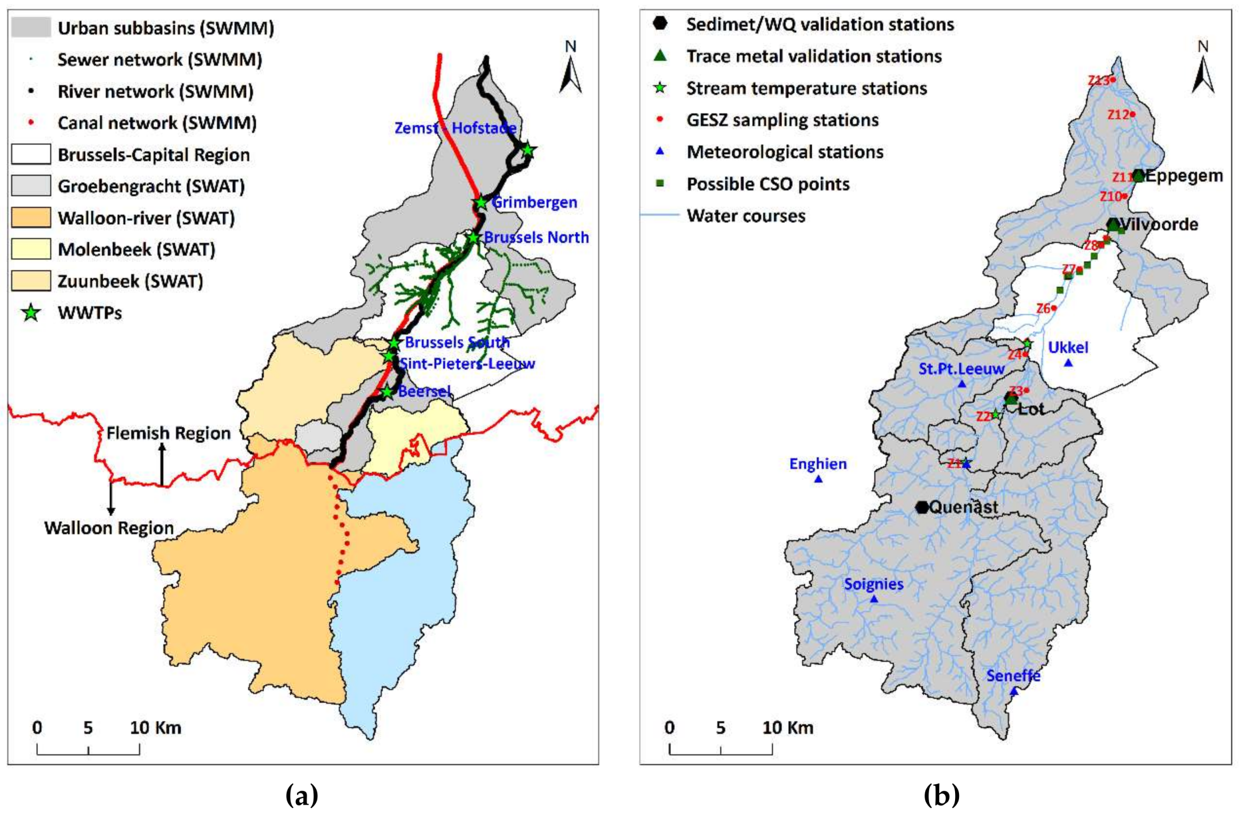
Figure 2.
Model components of the integrated trace metal transport model and the data exchange between the components in Open Modelling Interface (OpenMI).
Figure 2.
Model components of the integrated trace metal transport model and the data exchange between the components in Open Modelling Interface (OpenMI).
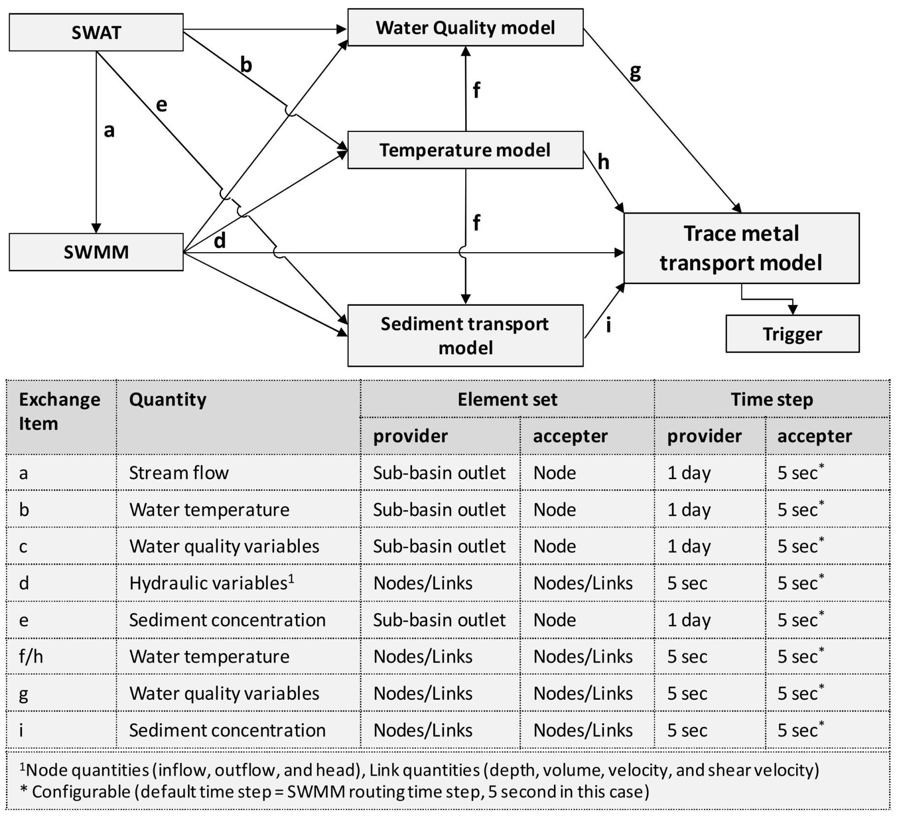
Figure 3.
Box plots of the total metal concentrations at the outlet of waste water treatment plants (WWTPs) (top row) and at Good Ecological Status of the river Zenne (GESZ) station Z13, near the river outlet (bottom row), measured during the GESZ sampling campaigns.
Figure 3.
Box plots of the total metal concentrations at the outlet of waste water treatment plants (WWTPs) (top row) and at Good Ecological Status of the river Zenne (GESZ) station Z13, near the river outlet (bottom row), measured during the GESZ sampling campaigns.
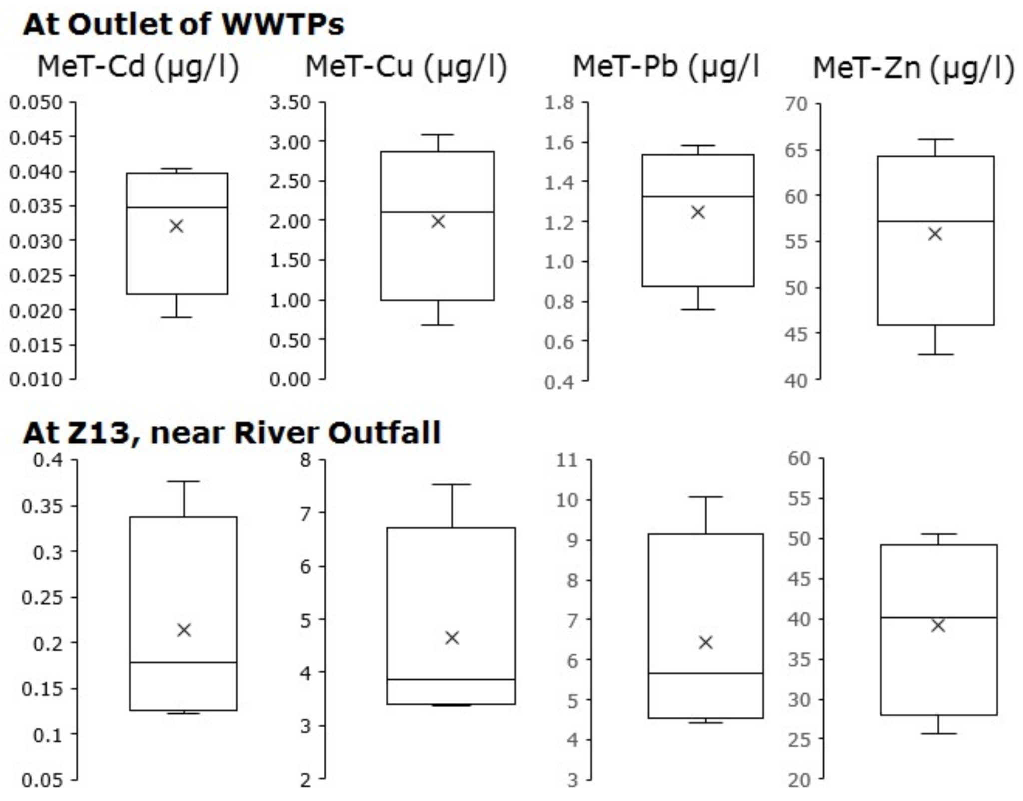
Figure 4.
Predicted versus observed (a) total concentrations: MeT (b) Partitioning coefficients (log based: Log Kd) of Cd, Cu, Pb and Zn based on multi-linear regression (MLR) (circles) and principle component regression (PCR) (triangles). Dotted lines indicate the 1-standard deviation prediction interval. The solid lines correspond to the bisector lines.
Figure 5.
Multi-linear regression (MLR) and principle component regression (PCR) based simulated (daily aggregated) and observed total (MeT), dissolved (MeD) and particulate (MeP) metal concentration for Cu, Cd, Zn and Pb for the time frame of 2007–2010.
Figure 5.
Multi-linear regression (MLR) and principle component regression (PCR) based simulated (daily aggregated) and observed total (MeT), dissolved (MeD) and particulate (MeP) metal concentration for Cu, Cd, Zn and Pb for the time frame of 2007–2010.


Table 1.
Concentration limits imposed by different legislation.
| Species | Unit | EU WFD | US EPA | Flemish Level # | |
|---|---|---|---|---|---|
| Cd * | total | µg/L | - | 5 c | 8 |
| dissolved | 0.08–0.25 a,† | 0.72 d (1.8 $) | 0.08–0.25 † | ||
| Cu | total | µg/L | - | 1300 c | 30 |
| dissolved | 5–112 b,† | - | 7 | ||
| Pb ** | total | µg/L | - | 15 c | 50 |
| dissolved | 7.2 a | 2.5 d (65 $) | 7.2 | ||
| Zn | total | µg/L | 30–500 b,^, 300–2000 b,^^ | 5000 c | 200 |
| dissolved | - | 120 d,$ | 20 | ||
* Priority hazardous substance; ** Priority substance; † Depending on hardness as expressed in mgCaCO3/l; EU WFD: European Union Water Framework Directive; a EQS: Environmental Quality Standard, yearly average value EU [2]; Directive 2008/105/EC; b Quality of fresh waters to support fish life, yearly average value Directive 2006/44/EC EU [6]; ^ Salmonoid waters; ^^ Cyprinid waters; US EPA: United States Environmental Protection Agency; c Drinking water quality, based on instantaneous concentration US EPA [7]; d Aquatic Life Criteria US EPA [8], criterion continuous concentration. $ Criterion maximum concentration; # Basic quality standard, and yearly average value for rivers and oceans VLAREM [9].
Table 2.
Model inputs for the integrated model.
| Input | Value/Resolution | Remarks/References |
|---|---|---|
| A. SWAT | ||
| Digital Elevation Model (DEM) | 30 × 30 m | ASTER GDEM 1, DHM-OC GIS Vlaanderen |
| Soil map | 20 × 20 m | Carte Numérique des Sols de Wallonie (CNSW) 2, VLM-OC GIS Vlaanderen |
| Landuse map | 20 × 20 m | Corrine (Walloon region), VLM-OC GIS Vlaanderen |
| Hydro-meteorological data (Rainfall, relative humidity, wind speed, solar radiation, temperature) | daily | Royal Meteorological Institute of Belgium (RMI), Direction Générale opérationnelle de la mobilité et des Voies Hydrauliques (DGVH) 3, Vlaamse Milieumaatschappij (VMM) 4 |
| Fertilizer application | Seasonal 5 | Direction Générale Opérationnelle Agriculture, Ressources Naturelles et Environnement (DGARNE) 6, Vlaamse Landmaatschappij (VLM) 7 |
| Point sources | yearly/constant | Société Publique de la Gestion de l’Eau (SPGE) 8 |
| B. SWMM | ||
| River/Canal logitudinal profile and cross section geometry | ca. 100 m | Waterbouwkundig Laboratorium 9 |
| River logitudinal profile and cross section geometry | ca. 100 m | Waterbouwkundig Laboratorium 9 |
| WWTP-Brussels-North sewer system geometry | ca. 100 m | Translated from a hydraulic model HYSTEM-EXTRAN built by Department of Hydrology and Hydraulic Entgineering, Vrije Universiteit Brussel |
| Rainfall | hourly | Royal Meteorological Institute of Belgium (RMI) 10, Société Bruxelloise de Gestion de l’Eau-Brusselse Maatschappij voor Waterbeheer (SBGE/BMWB) 11 |
| Tide levels at outlet | 30 min | Waterbouwkundig Laboratorium 9 |
| Boundary flows at tributaries | daily | SWAT simulated |
| C. Temperature model | ||
| Air temperature | daily | Royal Meteorological Institute of Belgium (RMI) 10 |
| Temperature of WWTP effluent | 20 °C | Constant (Based on GESZ measurements) 12 |
| Temperature of CSO points | 15 °C | Constant (assumed) |
| D. Sediment transport model | ||
| Sediment concentration at tributaries | daily | SWAT simulated |
| Sediment concentration at WWTP outlets | daily | Observed series (Aquiris 13, Vivaqua 14, Aquafin 15) |
| Sediment concentration at CSO points | 207 mg/L | Constant (Based on GESZ measurements) 12 |
| Sediment concentration at outlet | 8.1 mg/L | Constant (Based on GESZ measurements) 12 |
| Particle size distributions, PSDs | - | Based on GESZ measurement 12, constant |
| E. Water Quality model | ||
| Water quality concentration at tributaries | daily | SWAT simulated |
| Water quality concentration at WWTP outlets | weekly | Observed series (Aquiris 13, Vivaqua 14, Aquafin 15) |
| Water quality concentration at CSO points | - | Constant (Based on GESZ measurements) 12 |
| Water quality concentration at river outlet | - | Constant (Based on GESZ measurements) 12 |
| F. Trace metal model | ||
| Trace metal concentration at tributaries | - | Based on MLR and PCA regression |
| Trace metal concentration at WWTP outlets | - | Constant (Based on GESZ measurements) 12 |
| Trace metal concentration at CSO points | - | Constant (Based on GESZ measurements) 12 |
| Trace metal concentration at river outlet | - | Constant (Based on GESZ measurements) 12 |
1 http://www.gdem.aster.ersdac.or.jp/search.jsp; 2 http://cartographie.wallonie.be/NewPortailCarto/; 3 http://voies-hydrauliques.wallonie.be; 4 http://www.hydronet.be; 5 Considered to be typically applied from February to August of every year; 6 http://environnement.wallonie.be/; 7 http://www.vlm.be/; 8 http://www.spge.be/; 9 http://www.watlab.be/nl; 10 http://www.meteo.be/meteo/view/en/65239-Home.html; 11 http://www.sbge.be/; 12 GESZ measurement: observed during GESZ sampling campaigns at different stations (Figure 1, right); 13 http://www.aquiris.be/; 14 http://www.vivaqua.be/; 15 http://www.aquafin.be/nl/.
Table 3.
The Good Ecological Status of the river Zenne (GESZ) sampling campaigns.
| Group | Date/Period | Locations | Samples | Remarks |
|---|---|---|---|---|
| Group 1 | 30 September–1 October 2009 | GESZ sampling stations (Z1–Z13), outlets of canals and tributaries, WWTP Brussels South and North. | 16 | During dry weather conditions (DWFs) |
| 26–27 April 2010 | 17 | |||
| 6–7 Jul 2010 | 17 | |||
| 26–27 October 2010 | 17 | |||
| 16–17 September 2010 | GESZ sampling stations (Z4, Z7 and Z9) | 46 | 24-hcampaign | |
| Group 2 | 15–16 December 2009 | Z4 to Z13 | 7 | During dry weather conditions (DWFs) |
| 16 June 2011 | Z9 | 22 | 30-min measurement at wet weather |
Table 4.
Summary of total metal concentration (MeT) and partitioning coefficient (log based: LogKd) regression equations using the multi-linear regression (MLR) and principle component regression (PCR) techniques at rural catchment runoff discharging points.
Table 4.
Summary of total metal concentration (MeT) and partitioning coefficient (log based: LogKd) regression equations using the multi-linear regression (MLR) and principle component regression (PCR) techniques at rural catchment runoff discharging points.
| Dependent Variable | Regression Type | Regression Equations | R2 | Press |
|---|---|---|---|---|
| MeT-Cd | MLR | 3 (EC, pH, SPM) 267.72 − 179.48 × EC − 1.35 × pH × SPM + 14.46 × SPM | 0.26 | 328 |
| PCR | 3 (3 components) 0.17 × F3 − 0.32 × F4 − 0.33 × F5 | 0.26 | 76 | |
| MeT-Cu | MLR | 2 (EC, SPM) −2.38 − 22.26 × EC × SPM + 36.61 × SPM | 0.42 | 24 |
| PCR | 9 (7 components) 0.15 × F1 + 0.03 × F1 × F2 − 0.09 × F1 ×F3 − 0.18 × F1 × F5 − 0.07 × F2 + 0.25 × F3 − 0.27 × F4 − 0.39 × F5 − 1.945 × F7 | 0.59 | 58 | |
| MeT-Pb | MLR | 4 (EC, SPM, Ts, pH) 266.7 − 173.2 × EC + 2.36 × SPM + 0.05 × Ts − 0.006 × Ts × pH | 0.42 | 42 |
| PCR | 5 (4 components) 0.1291 × F1 − 0.1698 ×F1 × F5 + 0.2224 × F3 − 0.1538 × F4 − 0.6083 × F5 | 0.46 | 62 | |
| MeT-Zn | MLR | 3 (EC, pH, SPM) 50.76 − 31.99 × EC − 0.31 × pH × SPM + 3.24 × SPM | 0.39 | 8 |
| PCR | 5 (4 components) −0.07031 × F2 × F3 − 0.7675 × F2 × F4 + 0.1849 × F3 − 0.4553 × F4 − 0.3606 × F5 | 0.41 | 68 | |
| LogKd-Cd | MLR | 5 (MeTCd, EC, SO2, SPM) 217.4 − 0.24 × MeTCd − 135.2 × EC + 0.05 × SO2 × MeTCd + 0.17 × SPM × MeTCd | 0.55 | 19 |
| PCR | 7 (5 components) 5.54 + 0.08 × F2 + 0.03 × F2 × F3 + 0.13 × F2 × F7 + 0.14 × F3 − 0.05 × F3 × F6 + 0.21 × F5 − 0.25 × F6 | 0.65 | 17 | |
| LogKd-Cu | MLR | 6 (MeTCu, SO2, pH, SPM) 10.15 − 1.187 × MeTCu + 0.36 × SO2 × SPM − 0.11 × pH × O2 − 2.7 × SPM + 0.91 × SPM × MeTCu | 0.52 | 14 |
| PCR | 11 (7 components) 5.43 − 0.056 × F1 + 0.0098F1 × F2 − 0.094 × F1 × F7 + 0.087 × F2 − 0.109 × F4 + 0.1189 × F5 − 0.0483 × F7 | 0.53 | 15 | |
| LogKd-Pb | MLR | 4 (MeTPb, pH, SPM) 8.46 + 0.26 × pH × SPM − 3.69 × SPM + 0.27 × SPM × MeTPb | 0.49 | 15 |
| PCR | 6 (5 components) 6.04 + 0.05 × F1 + 0.008 × F1 × F2 + 0.05 × F2 + 0.06 × F3-0.12 × F4 + 0.17 × F5 | 0.51 | 16 | |
| LogKd-Zn | MLR | 2 (EC, Ts) 177.62 − 110.9 × EC + 0.002 × Ts × EC | 0.19 | 27 |
| PCR | 11 (7 components) 4.93 + 0.149 × F5 − 0.333 × F6 − 0.368 × F7 − 0.11 × F5 × F6-0.143 × F5 × F7 + 0.176 × F6 × F7 | 0.28 | 25 |
MLR: Multilinear Regression; PCR: Principle Component Regression; MeT: Total metal concentration (μg/L); Kd: Distribution coefficient (l/kg); EC: Electrical Conductivity (μS/cm); SPM: Suspended Particulate Matter (mg/L); Ts: Stream water temperature (°C); DO: Dissolved Oxygen (mg/L); PRESS: Predicted Residual Sums of Squares.
Table 5.
Goodness-of-fit statistics and final performance rating of different model components of the integrated trace metal transport model.
Table 5.
Goodness-of-fit statistics and final performance rating of different model components of the integrated trace metal transport model.
| Variable | Station | Model | Period | Time Span | Obs. | RMSE | MAE | PBIAS (%) | RSR | NSE | Performance Rating # |
|---|---|---|---|---|---|---|---|---|---|---|---|
| Stream flows | Tubize *,*** | SWAT standalone | Cal. | 1998–2008 | 4018 | 1.28 | 0.60 | −7.58 | 0.46 | 0.79 | Very good |
| Val. | 1994–1997 | 1461 | 1.68 | 0.87 | 3.00 | 0.59 | 0.65 | Good | |||
| Lot *** | Integrated | Cal. | 2007–2008 | 731 | 1.45 | 0.79 | −11.39 | 0.53 | 0.72 | Good | |
| Val. | 2009–2010 | 730 | 2.17 | 1.44 | 47.72 | 0.95 | 0.11 | Unsatisfactory | |||
| Vilvoorde *** | Cal. | 2007–2008 | 731 | 1.23 | 0.80 | 0.29 | 0.39 | 0.85 | Very good | ||
| Val. | 2009–2010 | 730 | 2.35 | 1.66 | −3.38 | 0.58 | 0.65 | Good | |||
| Eppegem *** | Cal. | 2007–2008 | 731 | 3.38 | 2.10 | 13.67 | 0.45 | 0.80 | Very good | ||
| Val. | 2009–2010 | 730 | 5.63 | 2.99 | 21.21 | 0.55 | 0.67 | Good | |||
| SPM † | Quenast | SWAT standalone | Cal. | 1998–2008 | 140 | 229.12 | 79.34 | −4.09 | 1.04 | −0.08 | Satisfactory |
| Val. | 1994–1997 | 49 | 121.92 | 52.93 | −11.99 | 1.54 | −1.38 | Satisfactory | |||
| Lot | Integrated | Cal. | 2007–2008 | 22 | 93.82 | 49.61 | 1.41 | 0.81 | 0.34 | Satisfactory | |
| Val. | 2009–2010 | 23 | 123.89 | 43.61 | 13.57 | 1.13 | −0.28 | Satisfactory | |||
| Vilvoorde | Cal. | 2007–2008 | 22 | 68.66 | 47.55 | −14.20 | 1.60 | −1.55 | Satisfactory | ||
| Val. | 2009-2010 | 36 | 87.77 | 45.83 | −6.06 | 1.03 | −0.05 | Satisfactory | |||
| Eppegem | Cal. | 2007–2008 | 22 | 63.28 | 45.09 | −27.31 | 2.31 | −4.32 | Satisfactory | ||
| Val. | 2009–2010 | 36 | 42.63 | 31.54 | −23.69 | 2.20 | −3.86 | Satisfactory | |||
| Ts † | U/S Brussels | Standalone | Cal. | 1990–2010 | 626 | 2.61 | 2.09 | −3.16 | 0.51 | 0.74 | Good |
| Lot | Integrated | Val. | 2007–2010 | 47 | 2.26 | 1.79 | 20.51 | 0.39 | 0.85 | Very good | |
| Vilvoorde | 72 | 1.74 | 1.47 | −10.53 | 0.35 | 0.88 | Very good | ||||
| Eppegem | 75 | 1.47 | 1.25 | −11.78 | 0.3 | 0.91 | Very good | ||||
| DO † | Quenast | SWAT standalone | Cal. | 1998–2008 | 171 | 0.90 | 0.66 | −15.27 | 0.97 | 0.06 | Satisfactory |
| Val. | 1994–1997 | 36 | 2.83 | 2.10 | −25.71 | 1.31 | −0.75 | Unsatisfactory | |||
| GESZ St. | Integrated | Cal. | ** | 13 | 0.86 | 0.72 | −11.46 | 0.86 | 0.26 | Satisfactory | |
| Lot | Val. | 2007–2010 | 45 | 1.44 | 1.20 | 10.63 | 0.61 | 0.63 | Good | ||
| Vilvoorde | 66 | 2.23 | 1.71 | −1.32 | 1.19 | −0.41 | Satisfactory | ||||
| Eppegem | 70 | 2.59 | 2.23 | 47.56 | 1.08 | −0.16 | Unsatisfactory | ||||
| pH † | GESZ St. | Integrated | Cal. | ** | 13 | 0.24 | 0.20 | −2.21 | 2.28 | −4.21 | Satisfactory |
| Lot | Val. | 2007–2010 | 45 | 0.60 | 0.58 | −9.16 | 3.72 | −12.87 | Satisfactory | ||
| Vilvoorde | 70 | 0.26 | 0.20 | −1.32 | 1.19 | −0.41 | Satisfactory | ||||
| Eppegem | 74 | 0.19 | 0.14 | −0.93 | 1.15 | −0.32 | Satisfactory | ||||
| EC † | GESZ St. | Integrated | Cal. | ** | 13 | 142.91 | 88.24 | −0.05 | 0.69 | 0.52 | Good |
| Lot | Val. | 2007–2010 | 46 | 171.05 | 133.20 | 0.17 | 1.32 | −0.74 | Satisfactory | ||
| Vilvoorde | 70 | 334.13 | 218.43 | 0.07 | 1.03 | −0.06 | Satisfactory | ||||
| Eppegem | 73 | 363.58 | 273.97 | −0.05 | 1.02 | −0.03 | Satisfactory | ||||
| MeT-Cu † | Lot | Int.-MLR | Val. | 2007–2010 | 13 | 7.29 | 6.02 | −14.78 | 1.31 | −0.70 | Satisfactory |
| Int.-PCR | 10.49 | 7.30 | −0.44 | 1.24 | −0.53 | Satisfactory | |||||
| Vilvoorde | Int.-MLR | 43 | 14.19 | 10.03 | −2.42 | 0.98 | 0.05 | Satisfactory | |||
| Int.-PCR | 14.42 | 10.17 | −2.38 | 0.94 | 0.11 | Satisfactory | |||||
| Eppegem | Int.-MLR | 41 | 17.49 | 11.61 | 12.41 | 1.28 | −0.65 | Satisfactory | |||
| Int.-PCR | 15.40 | 10.37 | 3.97 | 1.21 | −0.47 | Satisfactory | |||||
| MeT-Cd † | Vilvoorde | Int.-MLR | Val. | 2007–2010 | 23 | 0.31 | 0.25 | 6.19 | 1.20 | −0.45 | Satisfactory |
| Int.-PCR | 0.61 | 0.33 | 16.25 | 1.14 | −0.30 | Satisfactory | |||||
| Eppegem | Int.-MLR | 25 | 0.30 | 0.19 | 25.16 | 1.16 | −0.35 | Satisfactory | |||
| Int.-PCR | 0.28 | 0.18 | 18.94 | 1.21 | −0.45 | Satisfactory | |||||
| MeT-Zn † | Lot | Int.-MLR | Val. | 2007–2010 | 26 | 72.60 | 44.64 | 11.70 | 1.07 | −0.16 | Satisfactory |
| Int.-PCR | 111.05 | 70.38 | 17.81 | 1.69 | −1.86 | Satisfactory | |||||
| Vilvoorde | Int.-MLR | 55 | 78.10 | 50.94 | 3.25 | 0.88 | 0.23 | Satisfactory | |||
| Int.-PCR | 91.12 | 64.27 | 4.93 | 1.13 | −0.27 | Satisfactory | |||||
| Eppegem | Int.-MLR | 49 | 105.68 | 69.60 | 8.65 | 1.31 | −0.71 | Satisfactory | |||
| Int.-PCR | 123.31 | 86.53 | 12.14 | 1.85 | −2.43 | Satisfactory | |||||
| MeT-Pb † | Vilvoorde | Int.-MLR | Val. | 2007–2010 | 55 | 21.97 | 13.00 | 5.98 | 0.86 | 0.26 | Satisfactory |
| Int.-PCR | 21.29 | 12.00 | 2.71 | 0.84 | 0.29 | Satisfactory | |||||
| Eppegem | Int.-MLR | 40 | 20.74 | 15.62 | 9.00 | 1.33 | −0.77 | Satisfactory | |||
| Int.-PCR | 19.00 | 13.82 | 3.19 | 1.26 | −0.59 | Satisfactory | |||||
| MeD-Pb † | Eppegem | Int.-MLR | Val. | 2007–2010 | 24 | 0.28 | 0.16 | 12.57 | 1.01 | −0.01 | Satisfactory |
| Int.-PCR | 0.27 | 0.18 | −2.28 | 1.12 | −0.26 | Satisfactory | |||||
| MeD-Zn † | Vilvoorde | Int.-MLR | Val. | 2007–2010 | 49 | 56.71 | 40.23 | 16.40 | 2.74 | −6.51 | Satisfactory |
| Int.-PCR | 85.74 | 48.41 | 8.26 | 3.05 | −8.32 | Satisfactory | |||||
| Eppegem | Int.-MLR | 30 | 96.04 | 44.59 | 30.28 | 3.46 | −11.00 | Unsatisfactory | |||
| Int.-PCR | 87.59 | 65.43 | 32.67 | 3.98 | −14.82 | Unsatisfactory | |||||
| Performance rating | PBIAS (%) (Stream flow) | PBIAS (%) (Metal) | RSR | NSE | Color Scheme | ||||||
| Very good | <±10 | <±15 | 0 to 0.5 | 0.75 to 1 | |||||||
| Good | ±10 to ±15 | ±15 to ±30 | 0.5 to 0.6 | 0.65 to 0.75 | |||||||
| Satisfactory | ±15 to ±25 | ±30 to ±55 | 0.6 to 0.7 | 0.5 to 0.65 | |||||||
| Unsatisfactory | >±25 | >±55 | >0.7 | <0.5 | |||||||
* Tubize is located approximately 4 km downstream of Quenast; ** Five GESZ sampling campaigns were conducted from September 2009 to October 2010; *** Based on daily time series; † Values were Box-Cox transformed before calculating statistics; # Based on Moriasi et al. [60] considering the PBIAS, RSR and NSE (see below); Obs.: Numbers of Observations; Cal.: Calibration; Val.: Validation; Int.: Integrated; U/S: Upstream; Ts: Stream Water Temperature; SPM: Suspended Particulate Matter; DO: Dissolved Oxygen; EC: Electrical Conductivity at 25 °C; MeT: Total Metal concentration; MeD: Dissolved Metal concentration.
Table 6.
Simulated yearly average concentration of different metal species at Lot, Vilvoorde and Eppegem and comparison with Flemish and European Union (EU) mandatory levels.
Table 6.
Simulated yearly average concentration of different metal species at Lot, Vilvoorde and Eppegem and comparison with Flemish and European Union (EU) mandatory levels.
| Lot | ||||||||||
|---|---|---|---|---|---|---|---|---|---|---|
| Metal Species | Flemish 1 | EU WFD 1 | 2007 | 2008 | 2009 | 2010 | ||||
| MLR | PCR | MLR | PCR | MLR | PCR | MLR | PCR | |||
| CdT | 8 | - | 0.16 | 0.17 | 0.21 | 0.48 | 0.22 | 0.23 | 0.34 | 0.68 |
| CdD | 0.09 | 0.09 | 0.003 | 0.014 | 0.002 | 0.015 | 0.002 | 0.012 | 0.002 | 0.013 |
| CuT | 30 | 3.77 | 5.53 | 4.80 | 7.56 | 4.92 | 7.58 | 6.93 | 10.38 | |
| CuD | 7 | 40 | 0.39 | 0.40 | 0.36 | 0.36 | 0.35 | 0.34 | 0.32 | 0.34 |
| PbT | 50 | - | 8.98 | 6.44 | 11.44 | 8.36 | 11.60 | 8.34 | 19.32 | 14.39 |
| PbD | 7.2 | 7.2 | 0.34 | 0.25 | 0.34 | 0.25 | 0.34 | 0.24 | 0.32 | 0.23 |
| ZnT | 200 | 300 | 61.20 | 103.08 | 77.64 | 116.31 | 78.34 | 126.00 | 108.77 | 177.02 |
| ZnD | 20 | - | 22.74 | 47.13 | 19.86 | 21.26 | 19.54 | 27.70 | 20.74 | 23.25 |
| Vilvoorde | ||||||||||
| CdT | 8 | - | 0.15 | 0.14 | 0.17 | 0.26 | 0.18 | 0.18 | 0.24 | 0.33 |
| CdD | 0.09 | 0.09 | 0.008 | 0.023 | 0.009 | 0.027 | 0.009 | 0.027 | 0.010 | 0.030 |
| CuT | 30 | 9.91 | 9.75 | 9.42 | 9.74 | 11.00 | 11.04 | 12.55 | 12.49 | |
| CuD | 7 | 40 | 0.85 | 0.71 | 0.91 | 0.72 | 0.88 | 0.63 | 1.00 | 0.74 |
| PbT | 50 | - | 12.08 | 11.12 | 12.25 | 11.01 | 14.85 | 13.56 | 16.87 | 14.73 |
| PbD | 7.2 | 7.2 | 0.20 | 0.23 | 0.22 | 0.26 | 0.20 | 0.24 | 0.22 | 0.25 |
| ZnT | 200 | 300 | 90.66 | 104.07 | 92.70 | 105.27 | 98.07 | 114.81 | 114.81 | 137.68 |
| ZnD | 20 | - | 60.73 | 59.38 | 63.02 | 60.41 | 62.98 | 66.78 | 73.49 | 77.57 |
| Eppegem | ||||||||||
| CdT | 8 | - | 0.17 | 0.17 | 0.18 | 0.14 | 0.20 | 0.20 | 0.26 | 0.37 |
| CdD | 0.09 | 0.09 | 0.013 | 0.036 | 0.015 | 0.039 | 0.015 | 0.042 | 0.017 | 0.043 |
| CuT | 30 | 14.13 | 10.98 | 13.10 | 10.05 | 14.76 | 11.73 | 15.78 | 13.09 | |
| CuD | 7 | 40 | 2.29 | 1.02 | 2.63 | 0.93 | 2.67 | 0.87 | 2.63 | 1.01 |
| PbT | 50 | - | 15.48 | 13.34 | 14.80 | 11.95 | 16.70 | 14.50 | 18.61 | 15.79 |
| PbD | 7.2 | 7.2 | 0.21 | 0.22 | 0.21 | 0.23 | 0.22 | 0.24 | 0.22 | 0.25 |
| ZnT | 200 | 300 | 92.19 | 162.50 | 91.89 | 122.12 | 99.76 | 143.59 | 115.90 | 166.38 |
| ZnD | 20 | - | 73.52 | 133.15 | 75.27 | 98.91 | 80.52 | 114.44 | 90.39 | 127.99 |
© 2018 by the authors. Licensee MDPI, Basel, Switzerland. This article is an open access article distributed under the terms and conditions of the Creative Commons Attribution (CC BY) license (http://creativecommons.org/licenses/by/4.0/).
Share and Cite
MDPI and ACS Style
Shrestha, N.K.; Punzal, C.; Leta, O.T.; Bauwens, W. Trace Metal Modelling of a Complex River Basin Using the Suite of Models Integrated in the OpenMI Platform. Environments 2018, 5, 48. https://doi.org/10.3390/environments5040048
AMA Style
Shrestha NK, Punzal C, Leta OT, Bauwens W. Trace Metal Modelling of a Complex River Basin Using the Suite of Models Integrated in the OpenMI Platform. Environments. 2018; 5(4):48. https://doi.org/10.3390/environments5040048
Chicago/Turabian StyleShrestha, Narayan Kumar, Chrismar Punzal, Olkeba Tolessa Leta, and Willy Bauwens. 2018. "Trace Metal Modelling of a Complex River Basin Using the Suite of Models Integrated in the OpenMI Platform" Environments 5, no. 4: 48. https://doi.org/10.3390/environments5040048
Note that from the first issue of 2016, this journal uses article numbers instead of page numbers. See further details here.