
Spatial and Temporal Variability Patterns of the Urban Heat Island in São Paulo


1
Center for Weather Forecasting and Climate Studies (CPTEC), National Institute for Space Research (INPE), São José dos Campos, SP 12227-010, Brazil
2
Universities Space Research Association/Goddard Earth Sciences Technology and Research (USRA/GESTAR), NASA Goddard Space Flight Center, Greenbelt, MD 29771, USA
*
Author to whom correspondence should be addressed.
Environments 2017, 4(2), 27; https://doi.org/10.3390/environments4020027
Submission received: 18 January 2017
/
Revised: 11 March 2017
/
Accepted: 22 March 2017
/
Published: 29 March 2017
Abstract
:The spatial and temporal variability patterns of the urban heat island (UHI) in the metropolitan area of Sao Paulo (MASP) were investigated using hourly temperature observations for a 10-year period from January 2002 to December 2011. The empirical orthogonal function (EOF) and cluster analysis (CA) techniques for multivariate analysis were used to determine the dominant modes of UHI variability and to identify the homogeneity between the temperature observations in the MASP. The EOF method was used to obtain the spatial patterns (T-mode EOF) and to define temporal variability (S-mode EOF). In the T-mode, three main modes of variability were recognized. The first EOF explained 66.7% of the total variance in the air temperature, the second explained 24.0%, and the third explained 7.8%. The first and third EOFs were associated with wind movement in the MASP. The second EOF was considered the most important mode and was found to be related to the level of urbanization in the MASP, the release of heat stored in the urban canopy and the release of heat by anthropogenic sources, thus representing the UHI pattern in the MASP. In the S-mode, two modes of variability were found. The first EOF explained 49.4% of the total variance in the data, and the second explained 30.9%. In the S-mode, the first EOF represented the spatial pattern of the UHI and was similar to the second EOF in the T-mode. CA resulted in the identification of six homogeneous groups corresponding to the EOF patterns observed. The standard UHI according to the scale and annual seasons for the period from 2002 to 2010 presented maximum values between 14:00 and 16:00 local time (LT) and minimum values between 07:00 and 09:00 LT. Seasonal analysis revealed that spring had the highest maximum and minimum UHI values relative to the other seasons.
1. Introduction
Urbanization produces significant changes in the radiative, thermal, and aerodynamic properties of surfaces by forming heat domes over cities, termed urban heat islands (UHIs) [1,2,3,4]. The spatial distribution of UHIs is typically marked by a strong horizontal temperature gradient at the urban–rural boundary and a gradual temperature decrease from the center to the edge of the city, and these gradients are strongly affected by local circulation and weather conditions; thus, they are defined by diurnal and seasonal variations [5,6,7].
The major contributing factors to the development and scale of the spatial patterns of UHIs include the scarcity of vegetation; the extensive use of waterproof, high thermal-capacity and/or albedo materials in construction and paving, thereby reducing evaporation; the typical three-dimensional geometry of the urban surface (canyon-type configuration), which traps energy; the size of the population; the release of anthropogenic heat through vehicle traffic, industrial processes, human and animal metabolism and energy consumption; and a high concentration of energy-absorbing pollutants (gases and aerosols) in the urban atmosphere. Furthermore, the spatial patterns of UHIs can be strongly influenced by surface characteristics, such as green areas, water bodies and local topographies [1,2,8,9,10,11,12,13,14,15,16,17,18,19].
The most widely recognized method of studying the spatial and temporal variability patterns of UHIs is by applying statistical techniques to observational meteorological databases [20,21,22,23,24]. This approach can analyze differences between urban and rural areas by comparing the intensity of the day and night UHI periods and by identifying variations at seasonal, interannual and decadal scales [25,26].
The metropolitan area of São Paulo (MASP) in southeast Brazil is among the top ten most highly populated cities and is one of the largest urban areas in the world. Previous attempts to determine the UHI patterns of the MASP have revealed that feedback occurs between the UHI and sea breezes [27,28,29]. According to Freitas et al. [29], the MASP’s UHI induces the formation of an active convergence zone in the city and accelerates the movement of the sea breeze front radially towards the urban center. The mixture of dry and warm urban air, with relatively damp and cold maritime air, favors convective instability and the development of intense convective cells, transporting a significant amount of humidity from the surface to upper levels, and only when the heat island dissipates, the sea breeze progresses beyond the city. The net effect is the retention of the sea breeze over the metropolitan area for up to two hours [29]. The UHI predominates during daytime, with the maximum and minimum intensities in the afternoon and morning, respectively [30]. However, during November, December, and January the minimum UHI intensity occurs at night. July and September exhibit the highest intensity, and June and November the lowest [30].
To the best of our knowledge, previous studies of the UHI of the MASP are all based on studies of climatological time series [31] and analyses of the effects of urbanization and morphology on temperature patterns [30,32,33]. Recent studies have also included remote sensing [34] and atmospheric modelling [29,35]. Other approaches have investigated the UHI according to its effects on comfort and human health; for example, areas with a more intense UHI (land surface temperature >32 °C) have a higher incidence of the disease dengue fever than other urban areas [36]. Nonetheless, the spatial and temporal patterns of urban temperatures and UHIs are not well understood for the largest metropolitan area of South America.
The main goal of this study was to determine the spatial and temporal structures of the UHI of the MASP. Specifically, we chose to investigate the diurnal, seasonal and interannual patterns, with a focus on the dominant modes of variability in air temperature anomaly data, to determine the characteristic similarities and differences in the MASP. Multivariate statistical analyses were performed using observational data. The study area, datasets and a review of the statistical analysis methods are described in Section 2, the results are presented and discussed in Section 3, and a summary and conclusions are provided in Section 4.
2. Materials and Methods
2.1. Study Area and Datasets
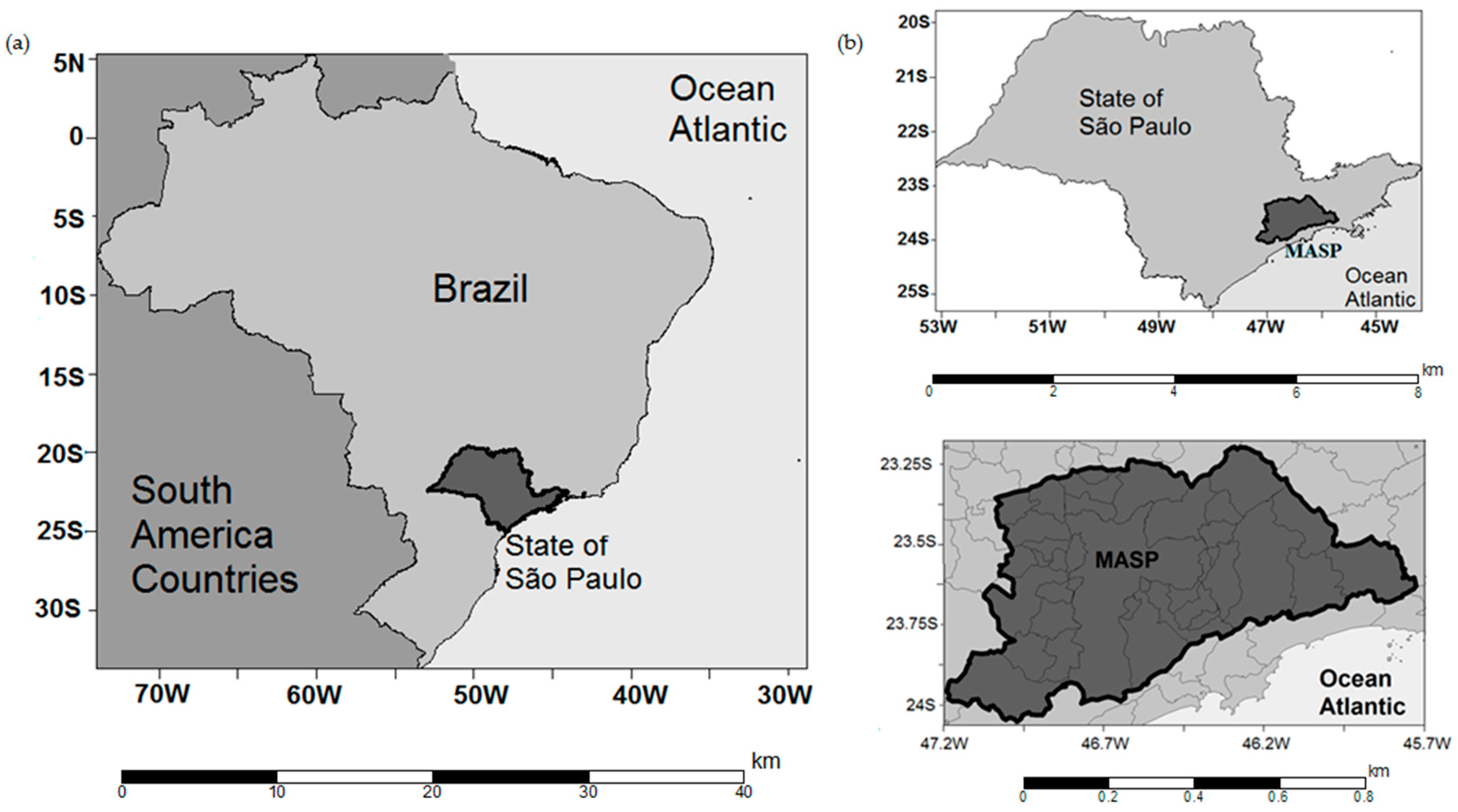
São Paulo city, in the southeast Brazil, is one of the most populated and largest urban conglomerates in South America (Figure 1a). The MASP consists of 39 cities (Figure 1b), and it is the largest hub of national wealth and the sixth largest city in the world. The MASP occupies a land area of 944 km2 and has a population of approximately 20 million (IBGE/2011).
The MASP has a topography dominated by hills ranging from 650 to 1200 m above the sea level (asl); the Mantiqueira and Serra do Mar Mountain chains standing out in the northern and southern limits of the region, respectively, and the Jaraguá Peak standing out at the west end of the Mantiqueira Mountains (Figure 2). São Paulo city is approximately 55 km from the Atlantic Ocean. The topography, the proximity to the ocean, and the intense urbanization significantly influence the pattern of atmospheric circulation and create peculiar weather conditions in the MASP.
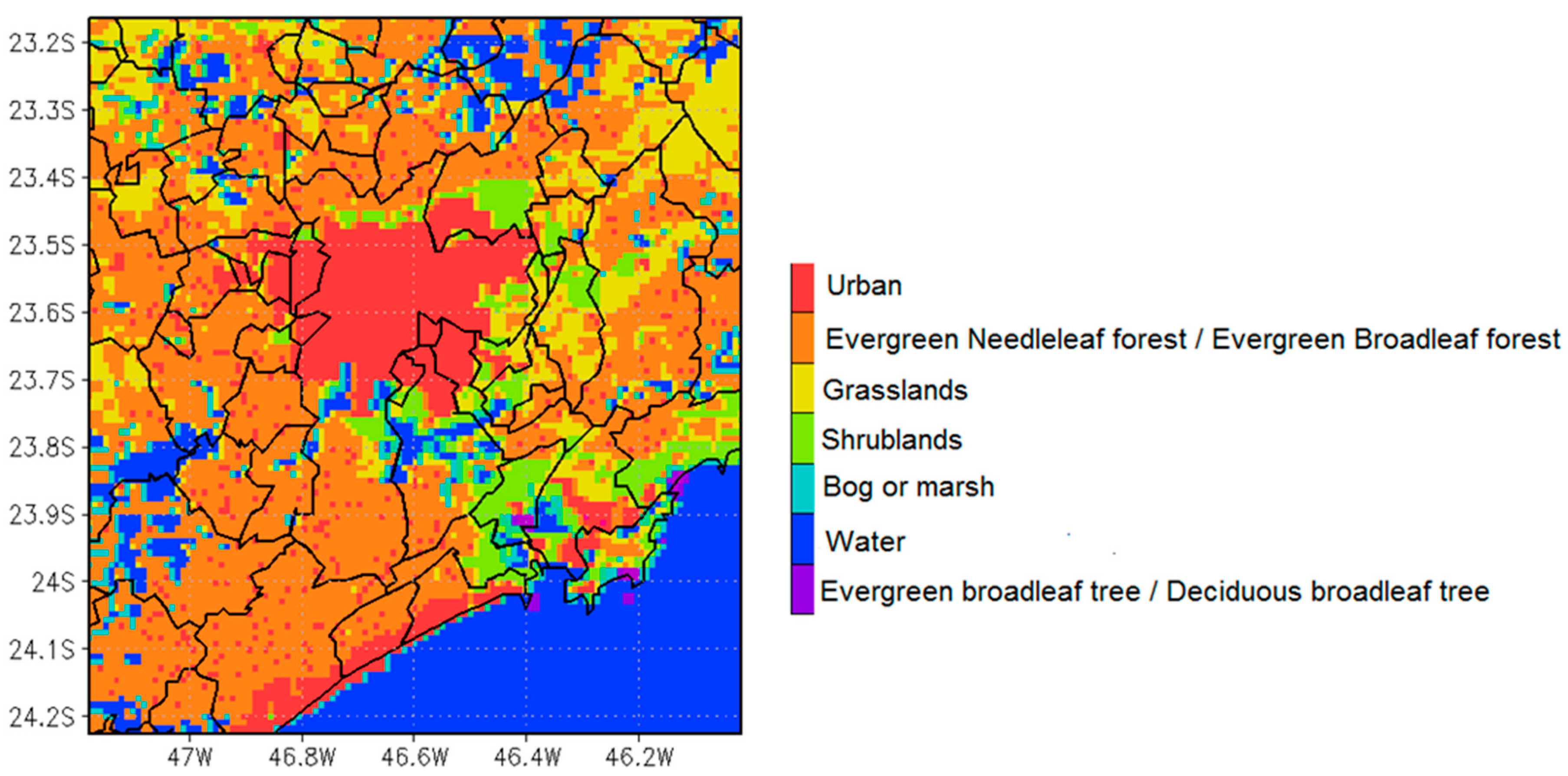
The MASP experienced a growth rate of 56% in the 30-year period from 1980 to 2010. There were nearly 12 million inhabitants in 1980, whereas in 2010 the population jumped to almost 21 million inhabitants (IBGE, 2010). The population growth triggered urban expansion at an accelerated rate. From 1962 to 2002, the urban area increased from 874 km2 to 2209 km2. Figure 3 shows a map of the current land use distribution in the MASP, highlighting the extensive urban area and the predominant types of land cover.
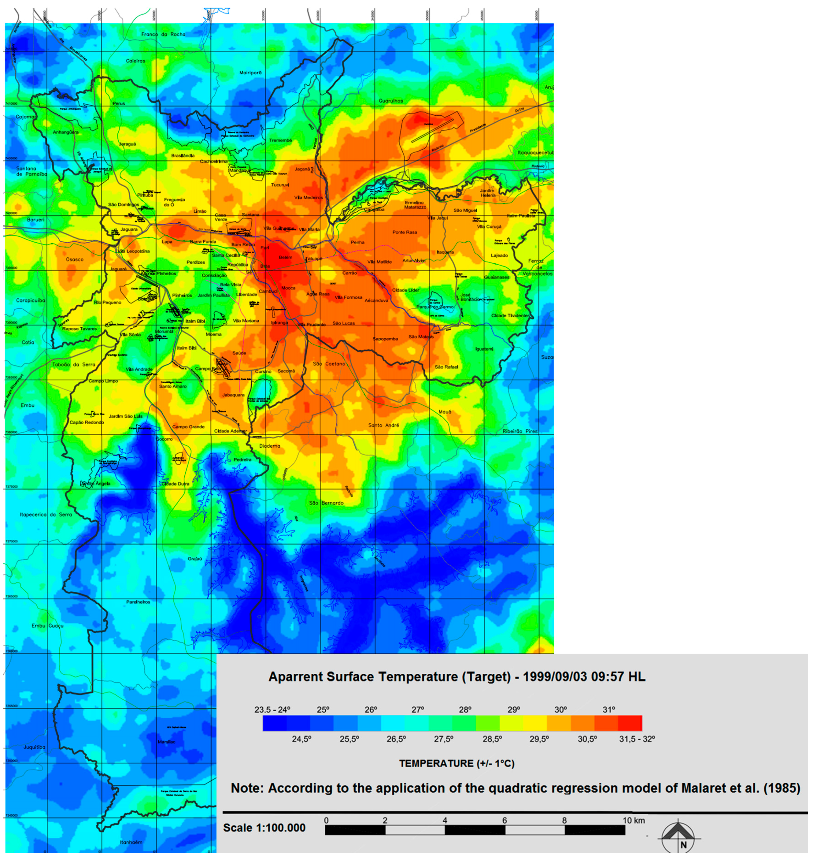
The large urban spot in the MASP (Figure 3) due to a rapid growth and unplanned urbanization produced several alterations of the natural landscape, which changed the surface energy fluxes and triggered dynamic and thermodynamic atmospheric changes, including the temperature pattern. The urbanization has promoted a heterogeneous distribution of surface temperatures in the MASP, with a warmer region in the nucleus and colder outer regions, which has led to the generation of various microclimates within this area. The map of apparent surface temperature in Figure 4, obtained by digital processing techniques of the high gain thermal band (TM6+) of the images captured by the LANDSAT-7 satellite sensor on 3 September 1999, illustrates the spatial distribution of these microclimates. This map reflects the quantitative spatial distribution of the apparent temperature, as it captures the emissivity of the surface and presents sensitivity to thermal contrasts. The processed image shows the areas with the highest apparent temperature of the surface (in red), in contrast to the cooler areas represented in blue. Temperatures range from about 24 °C to 32 °C. Detailed information is available at [37], last accessed 3 March 2017.
The analyzed database includes ten years of hourly air temperature observations from nine near-surface weather stations in the MASP from 2002 to 2011, with approximately 87,600 data points per station, hourly distributed. In total, the MASP dataset consists of 788,400 data points, in which approximately 244,304 (31%) are missing data. The missing data is however randomly distributed within the hours, days, and years. Therefore, no statistical method was used to fill the gaps in the dataset because these failures were not significant relative to the overall size of the dataset, or compromise its general pattern. Figure 5 depicts the locations of the MASP stations distributed within the 39 cities that compose the MASP (Figure 5a), and according to the land-use classification (Figure 5b). The weather stations available include conventional aerodrome stations (METAR code), automatic stations under the responsibility of the Environmental Protection Agency of the State of São Paulo (CETESB) and one automatic station operated by the University of São Paulo (USP). The spatial distribution of the meteorological stations with 10-year data available is not homogenous and does not cover the entire MASP. Therefore, we reduced the study to a smaller region with observational representativeness. In Figure 5a, the dark grey area illustrates the area under analysis in this study. Except for Parelheiros (number 9) and Guarulhos (number 6), which are in the transition region of urban area and shrublands, most stations are within the urban area.
In addition, we analyzed the correlation coefficients of the sea surface temperature (SST) anomalies between the Equatorial Pacific and southern Atlantic Oceans and the mean temperature anomalies observed in the MASP to investigate whether teleconnections affect the temporal variability of the urban temperature and to determine the related intensification or attenuation of the UHI. The SST data was from the ERA-Interim European Centre for Medium-Range Weather Forecasts (ECMWF) reanalysis data, with 1.5° × 1.5° horizontal resolution [39]. The monthly average SST grid data corresponds to the same 10-year period of the meteorological data (2002 to 2011).
2.2. Statistical Analysis
2.2.1. EOF Analysis
We applied the Empirical Orthogonal Function (EOF) analysis, also known as principal component analysis (PCA), to investigate the spatial and temporal variabilities in the UHI of the MASP. The EOF technique is one of the most widely used multivariate statistical techniques for atmospheric science analyses [40,41], and it became popular after Lorenz [42].
In this study, we employed the EOF technique to analyze the hourly mean temperature data over a 10-year period from January 2002 to December 2011. We subtracted the temperature at each station by the spatially averaged temperature in the MASP, therefore, linear combinations of temperature anomalies ( were used to calculate the Principal Components (PC’s). The EOF could be either based on analysis of the correlation matrix or the covariance matrix. In this study, we used the correlation matrix obtained from the standardized (n × K) anomalies matrix [Z], where K is the number of variables under analysis (temperature anomalies) and n is the number of observations from each weather station [43].
Depending on which parameters are selected, the EOF variables can be specified with different modes of decomposition. To obtain the spatial anomaly pattern, the T-mode EOF is used, and to define the temporal trend and variability of the grid points, the S-mode EOF is used [44,45,46,47,48,49,50]. In this study, we analyzed both the T-mode and S-mode EOFs to identify the characteristics of the spatial and temporal pattern and the temperature anomaly fields, respectively.
Detailed information about EOF analysis and about the T mode and S mode are in Appendix A.
2.2.2. Cluster Analysis
In addition to the EOF, we also applied the cluster analysis (CA). EOF and CA are useful tools for verifying how samples are related by determining the level of similarity with specific variables. CA is used to identify and classify objects/individuals based on their characteristics and to obtain similar groups. This analysis uses predetermined selection criteria to classify objects according to the similarities of elements to those within other groups [51,52].
In this study, regions of homogeneity were identified by arranging the temperature data in a (m × n) matrix, where m corresponds to the nine stations and n corresponds to the mean hourly temperature anomalies. Thus, CA was performed to provide a statistical description of the standard air temperature of each region to determine the temperature variability and weather patterns or local control factors in the MASP.
Detailed information about cluster analysis is in Appendix B.
2.2.3. Urban Heat Island Intensity
We calculated the UHI intensity (UHII) in the MASP based on differences in the mean hourly temperature between urban/suburban (Tu) areas and non-urban/vegetated (Tr) areas. This definition has been used in many studies, such as [25,53]:
Equation (1) is a traditional approach in which two stations (urban and vegetated) are applied to analyze the UHII. This approach is typically used when there are few stations in the study area. However, when there is only one station in the urban area and many stations in neighboring areas, the UHII is best defined as the difference between the urban station and a representative average of the countryside stations. When there are many stations within both the urban area and vegetated area, a representative station for the urban area should be carefully selected because significant variations usually occur within an urban area. In this study, we chose the representative stations in the urban and vegetated areas used for the UHII analysis after performing the CA.
3. Results
3.1. MASP Local Climate
For the 10-year period from January 2002 to December 2011, the average temperature of the MASP was 17 °C in the coldest month and 23 °C in the hottest month (Figure 6). Summer and spring months presented the highest solar radiation mean values (between 180 W/m2 and 200 W/m2), and winter months presented the lowest solar radiation mean values (approximately 100 W/m2). The mean spatial distribution of the 10-year temperature in the MASP was substantially uniform and ranged from 17 to 23 °C.
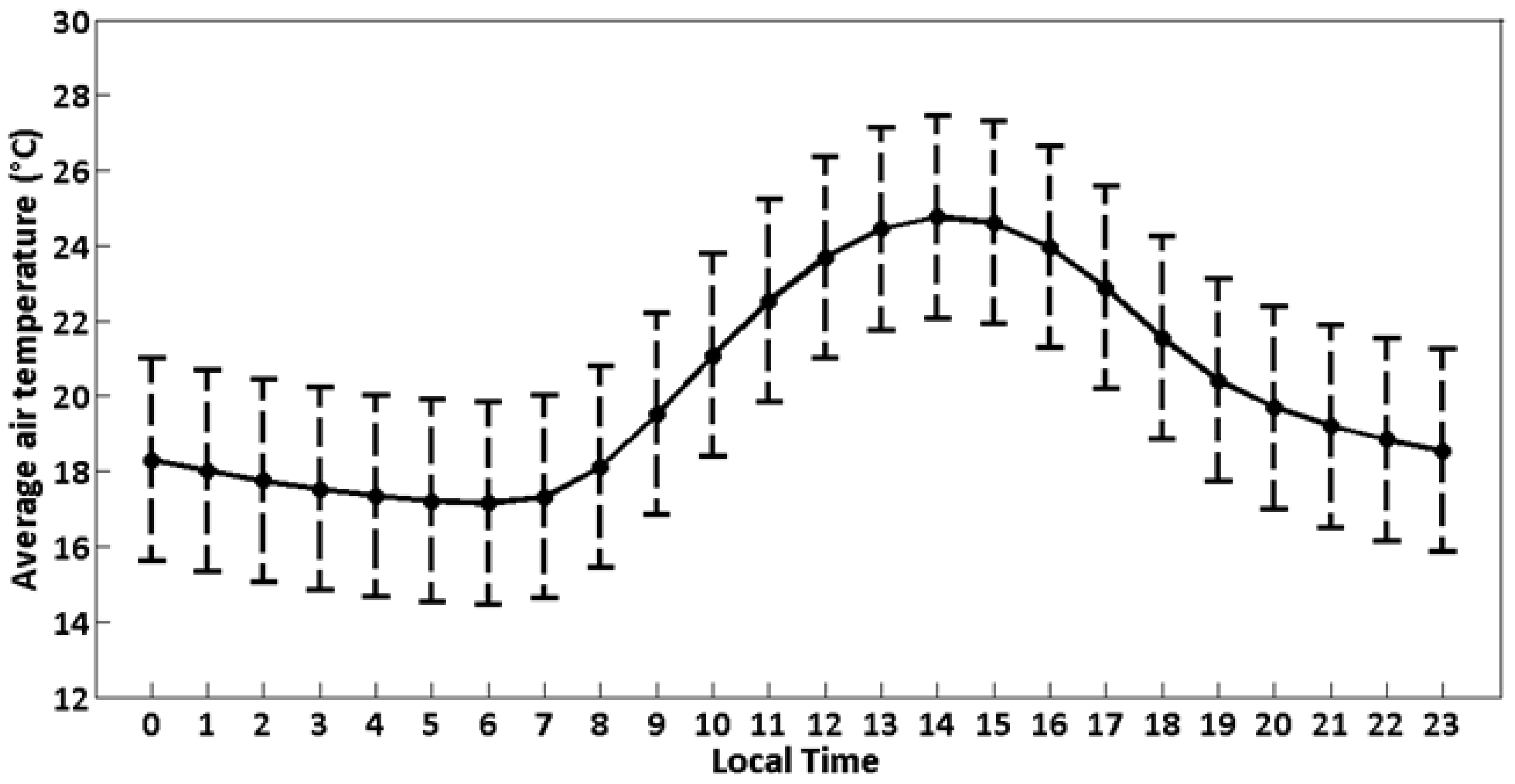
The 10-year mean diurnal temperature cycle in the MASP presented a peak of 25 °C at approximately 14:00 local time (LT) (Figure 7), primarily related to the solar radiation cycle, although also influenced by the high level of anthropogenic heat release. With the nighttime cooling, the temperature dropped to a minimum of 17 °C on average around 06:00 LT. Moreover, the daily cycle fluctuated with an amplitude of approximately 7.6 °C.
The sea breeze prevailing to the south/southeast, which corresponds to the oceanic/continental path that occurs during the daytime, strongly influences the wind regime in MASP, despite its 55 km distance from the coast (Figure 8). In addition, there was an eastern component throughout most of the region, which is most likely related to differential surface heating and the surface characteristics, such as the parks, water bodies, and more built-up environments. The wind speed in the MASP was typically low, ranging from 0.5 to 2.1 m/s.
3.2. EOF Analysis
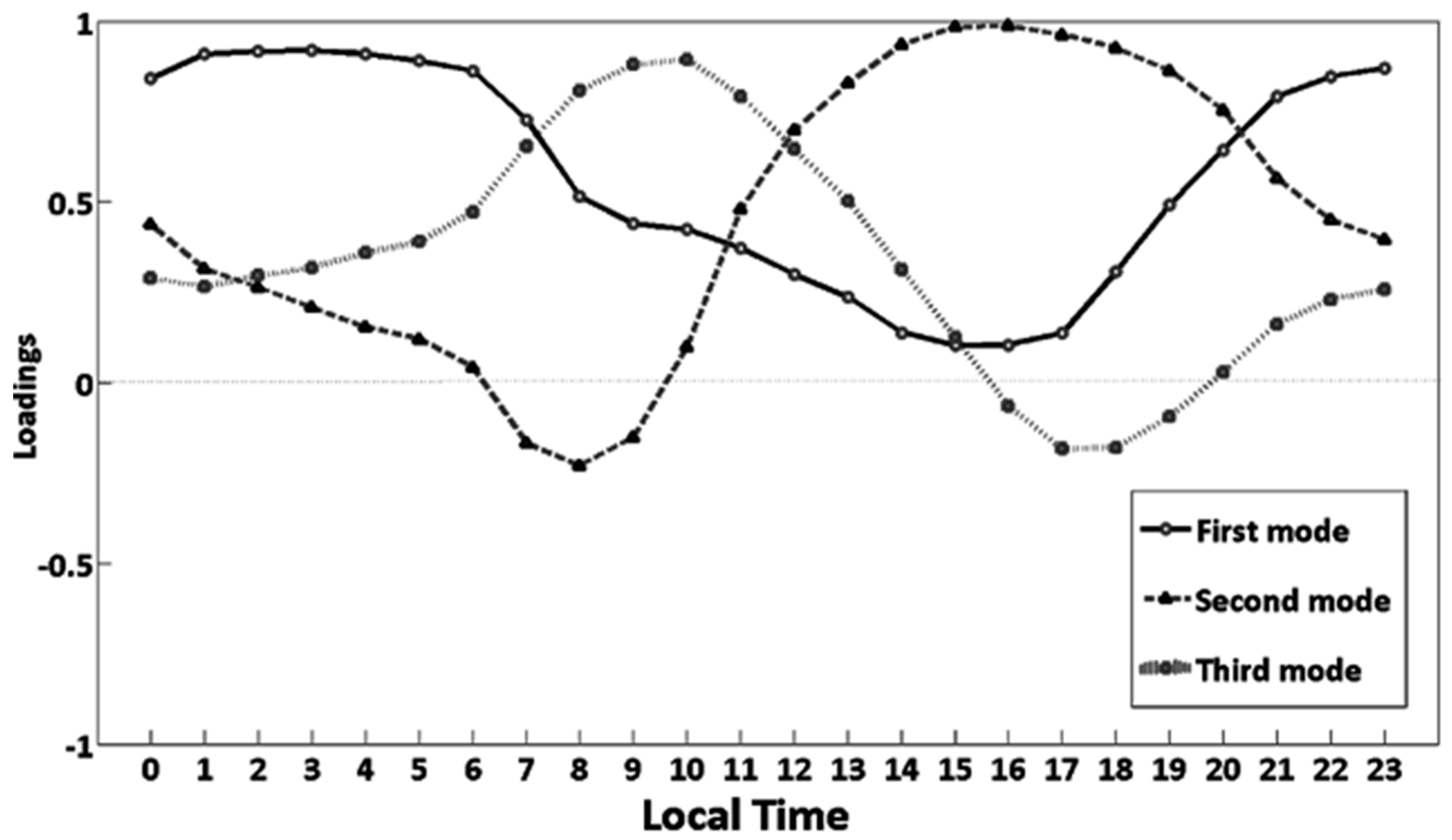
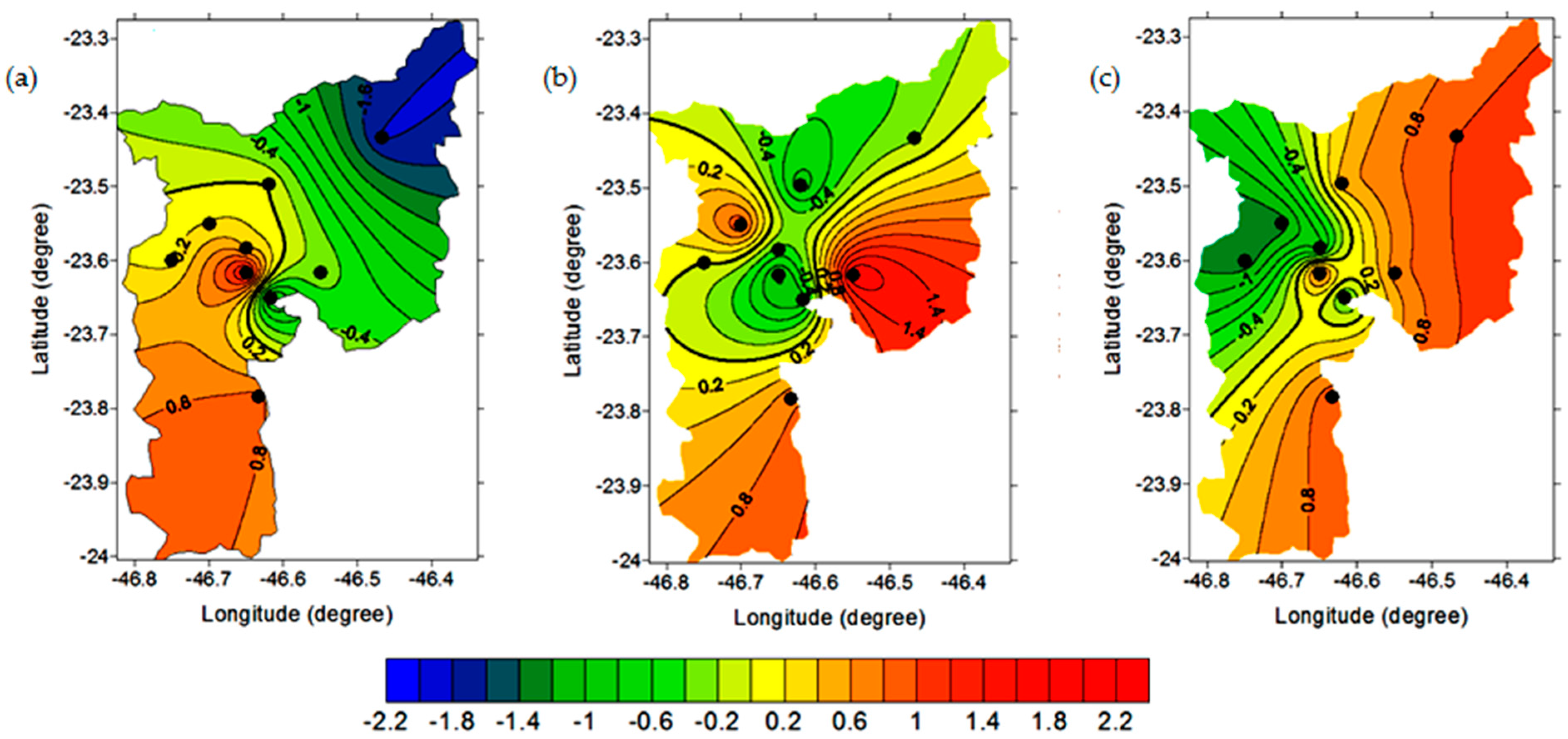
The T-mode EOF produced three dominant modes of temperature variability in the MASP, with the first, second and third EOFs together explaining approximately 99% of the total variance. The first mode (or the first PC score) explains 67% of the total variance and has a clear diurnal cycle. The temporal coefficient of the first mode or PC loadings (Figure 9) has the highest correlation (values greater than 0.8) between 00:00 and 06:00 and 21:00 and 23:00 LT. This result indicates that the late night and early morning periods are subject to a distinct spatial pattern. Thus, during these periods, a structural correspondence occurs in the temperature anomaly fields. The spatial structure associated with the first PC score (Figure 10a) has a dipole pattern with negative values in the east, north, and northwest MASP regions and positive values in the south MASP region. This pattern is associated with the MASP circulation mechanisms, representing the strong influence of the sea breeze with south and southeast winds in the southern part of the MASP, while in the north part prevailing the circulation of terrestrial breeze with east and northeast winds.
The second PC score explained 24% of the total variance, with the highest correlation values from 12:00 to 20:00 LT (Figure 9). The spatial structure of the second PC score had a pattern of negative and positive scores at the center and edges of the MASP, respectively (Figure 10b). Comparison of the spatial pattern of the temperature anomaly of the second PC (Figure 10b) with the map of the apparent surface temperatures of the MASP (Figure 4) revealed similarities in spatial behaviors, with the warmest regions coinciding with positive nuclei of the mode. The central region towards the northeast–southwest axis had a warmer core (Figure 4), and this region coincided with the central area in Figure 10b. The areas in Figure 4 that show colder core temperatures match the negative anomaly values of −0.2 to −0.6 in Figure 10b. Therefore, the second mode is associated with urbanization, representing the release of heat stored from urban areas as well as from other anthropogenic sources beyond the circulation process in the MASP. The second mode of the EOF is the one that better represents the UHI of the MASP.
The third mode explains 8% of the total variance, and the PC loading time series exhibits the highest correlation values from 07:00 to 11:00 LT (Figure 9). The third mode’s spatial structure (Figure 10c) is similar to that of the first mode because it also displays dipole behavior, although it displays positive values in the southwestern, southern, and eastern areas of the MASP and negative values in the northern and northwestern areas of the MASP region. The third EOF appears to be associated with the local circulation due to terrain or urban effects, and is therefore related to the first mode. It can be interpreted as a complementary representation of the wind circulation mechanisms in the MASP.
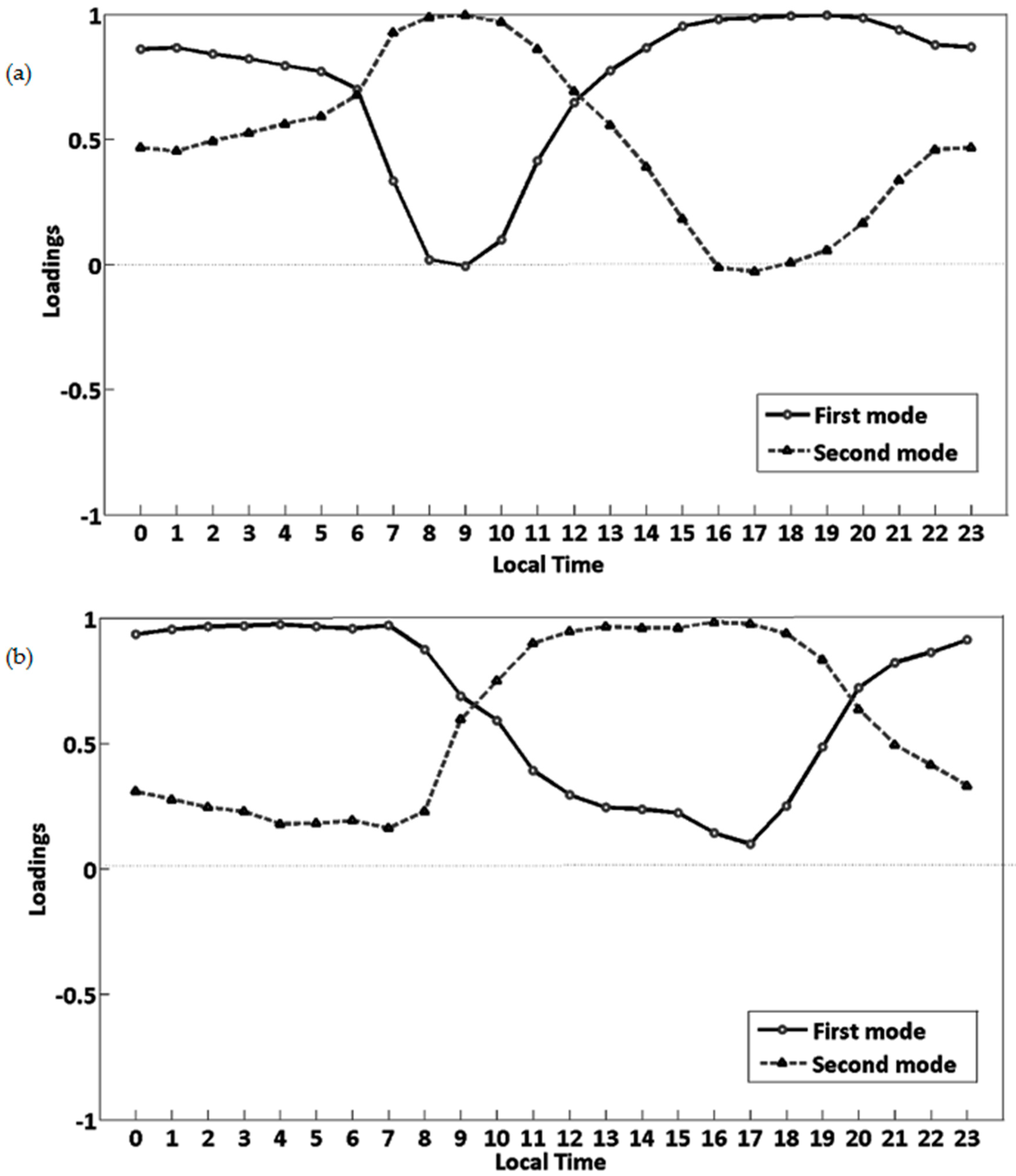
In the S-mode EOF, there were two dominant modes of variability, and they explained approximately 80% of the total variance. For the S-mode, the spatial pattern (or PC loading) of the variable under study shows the correlation fields determined by the PC score time series and all points in the spatial domain. The PC loading map shows the region(s) where the time series is representative of the temporal behavior of the temperature anomalies. Areas with low PC loadings do not correspond to the behavior of the original observations for that particular PC. The time series (or PC score) describes the principal types or patterns of temporal variability for the temperature anomaly [50].
The first PC (or first PC score) explained 49% of the total variance and had a clear diurnal cycle (Figure 11). The time series highlights the patterns of variability of the temperature anomalies during each period, with positive values between 00:00 and 11:00 LT and negative values between 12:00 and 23:00 LT. The spatial pattern of the first PC loading map (Figure 12a) is similar to that of the second PC of the T-mode EOF (Figure 10b), with positive values in the center and negative values at the edges of the MASP. The S-mode EOF demonstrates that the temperature anomaly in the center of the MASP is positive between 00:00 and 11:00 LT and negative otherwise, whereas the edge areas presented an inverted pattern, representing the temporal behavior of the MASP temperature anomaly. Therefore, the first PC of the S-mode corresponds to the spatial pattern of the UHI in the MASP, and it is similar to the second PC of the T-mode.
The second PC score pattern explains 31% of the total variance in temperature and also features a well-defined diurnal cycle (Figure 11). The temporal behavior of the second PC is similar to the first PC although advanced by 3 h. The dominant feature of the spatial structure of the second PC loading map (Figure 12b) is a positive structure on the west side of the MASP and negative structures elsewhere. Thus, on the western side of the MASP, the temperature anomaly is negative between 07:00 and 15:00 LT and positive otherwise. On the east side of the MASP, the temperature anomaly is positive from 07:00 to 15:00 LT and negative otherwise. This dipole pattern, also observed in the first and third PC of the T-mode EOF (Figure 10a,c), is associated with wind circulation in the MASP.
In summary, the second PC of the T-mode approach and the first PC of the S-mode approach represent the spatial pattern of the UHI in the MASP, whereas the first and third PCs of the T-mode approach and the second PC of the S-mode represent the wind circulation pattern in the MASP. According to Salles [47], similar results in both modes implies a simple linear spatial and temporal relationship that precludes other effects, such as dispersion, which occurs over time because of the non-linearity of real systems.
We also performed seasonal analysis of the spatial structures of the EOF for the T-mode EOF intending to obtain the spatial patterns of the temperature anomaly field and their sequences of occurrence throughout the year. The temporal and spatial patterns (Figure 13, Figure 14, Figure 15 and Figure 16) were similar to the T-mode patterns (Figure 9 and Figure 10). However, summer and winter only presented two modes (Figure 13 and Figure 14), whereas autumn and spring presented three modes (Figure 15 and Figure 16). During summer and winter, the first EOF mode explained 78% and 75% of the variance, and the second mode explained 17% and 20% of the variance, respectively. During fall and spring, the first EOF mode explained 69% and 55% of the total temperature variance, the second explained 23% and 28%, and the third explained 6% and 14%, respectively. This reduction in the number of variability modes is likely associated with a consolidated configuration of the thermodynamic properties of the atmosphere during summer and winter compared with those of the transition seasons in the MASP.
Another result that stands out in this seasonal analysis is the total variance representative of the variability modes of each season. During summer and winter, two dominant variability modes explain about 98% of the total variance, whereas in fall, three variability modes explain approximately 98% of the total variance, and in spring, three modes explain 97% of the variance. These differences between seasons and the different atmospheric thermodynamic patterns that occur at each station (as described above) may be associated with remote influences, which can increase the total variance in the transitional seasons relative to the other seasons. The most prominent remote influences that affect the southeastern part of Brasil are the El Niño-Southern Oscillation (ENSO), Madden-Julian Oscillation (MJO) and Pacific-South American (PSA) [54].
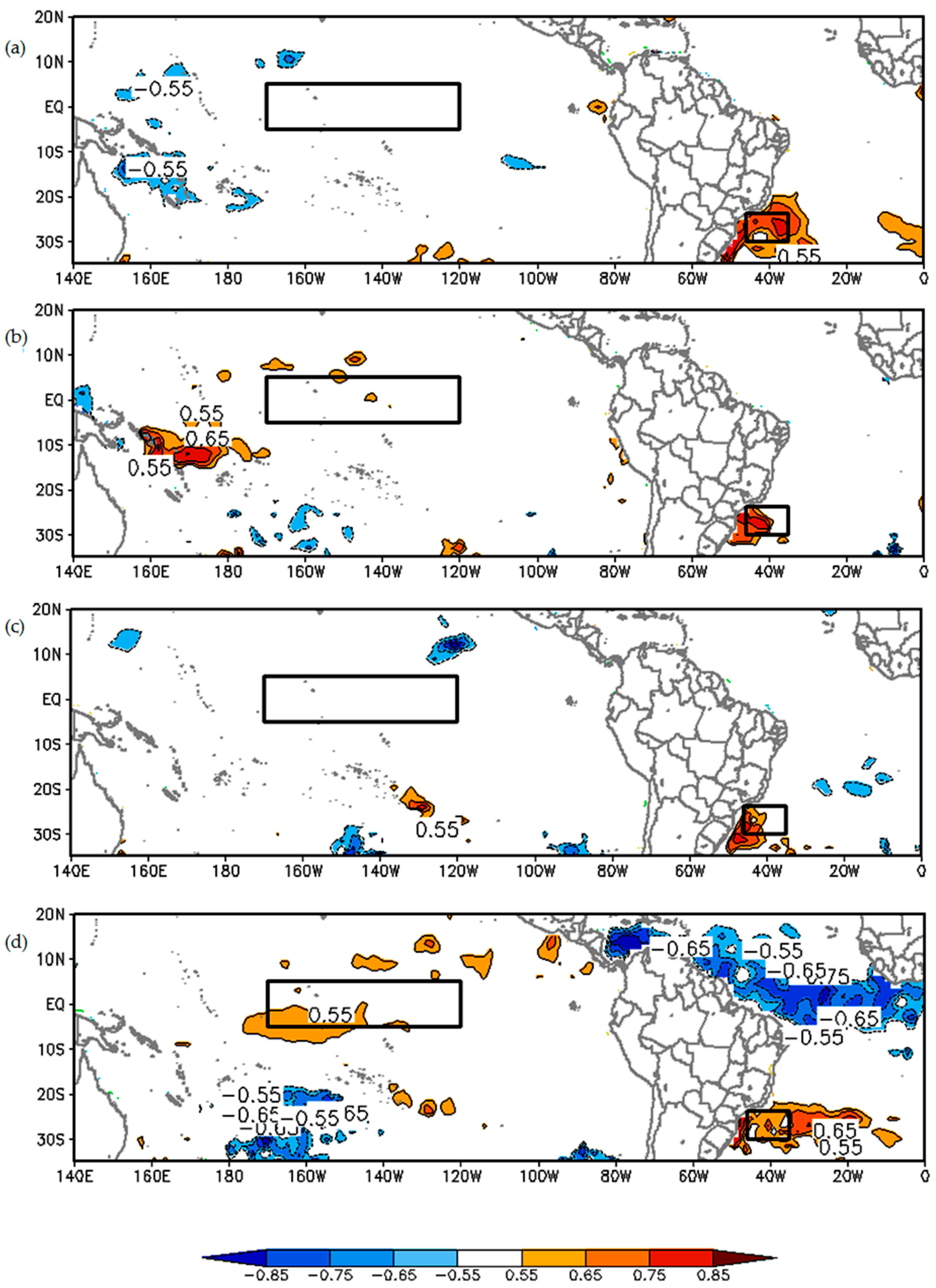
We analyzed the seasonal distribution of the correlation coefficients between the SST anomalies and the mean temperature anomalies observed in the MASP for the 10-year period (2002–2011) (Figure 17). We found an intense correlation between these two coefficients in the Atlantic Ocean area off the coast of southeast Brazil (anomaly marked as a square on the Atlantic Ocean near the MASP in Figure 17), which indicates that the MASP is primarily affected by the nearby ocean SST. The ENSO remote influence (square on the Equatorial Pacific Ocean in Figure 17) has no remote influence, except during fall and spring. During the transition seasons (Figure 17b,d) we detected a correlation, although weaker than the one with South Atlantic Ocean area, with the Niño 3.4 area. These results indicate that the seasonal factors in this area, such as the air temperature/UHI intensity in the MASP, as well as local-level phenomena, are also remotely influenced by the ENSO.
3.3. Cluster Analysis
The EOF methodology allowed the determination of the spatial patterns of temperature anomalies in the MASP, identifying warmer and cooler core areas as well as the temporal evolution of these spatial patterns throughout the day. Based on these results, we identified homogeneous regions or groups and determined the degree of similarity and differences among individual observations. Based on these results, we defined groups of stations that are similar. In the CA, the homogeneous groups should correspond with the groups observed in the spatial regionalization of the EOF analysis.
There is no theory or definition to determine the node heights in a CA dendrogram. As the goal is to gather stations with similar characteristics, we will not consider high-rescaled distances because they form large groups with high intra-cluster diversity. Therefore, we used 50% of the distance to determine the number of groups.
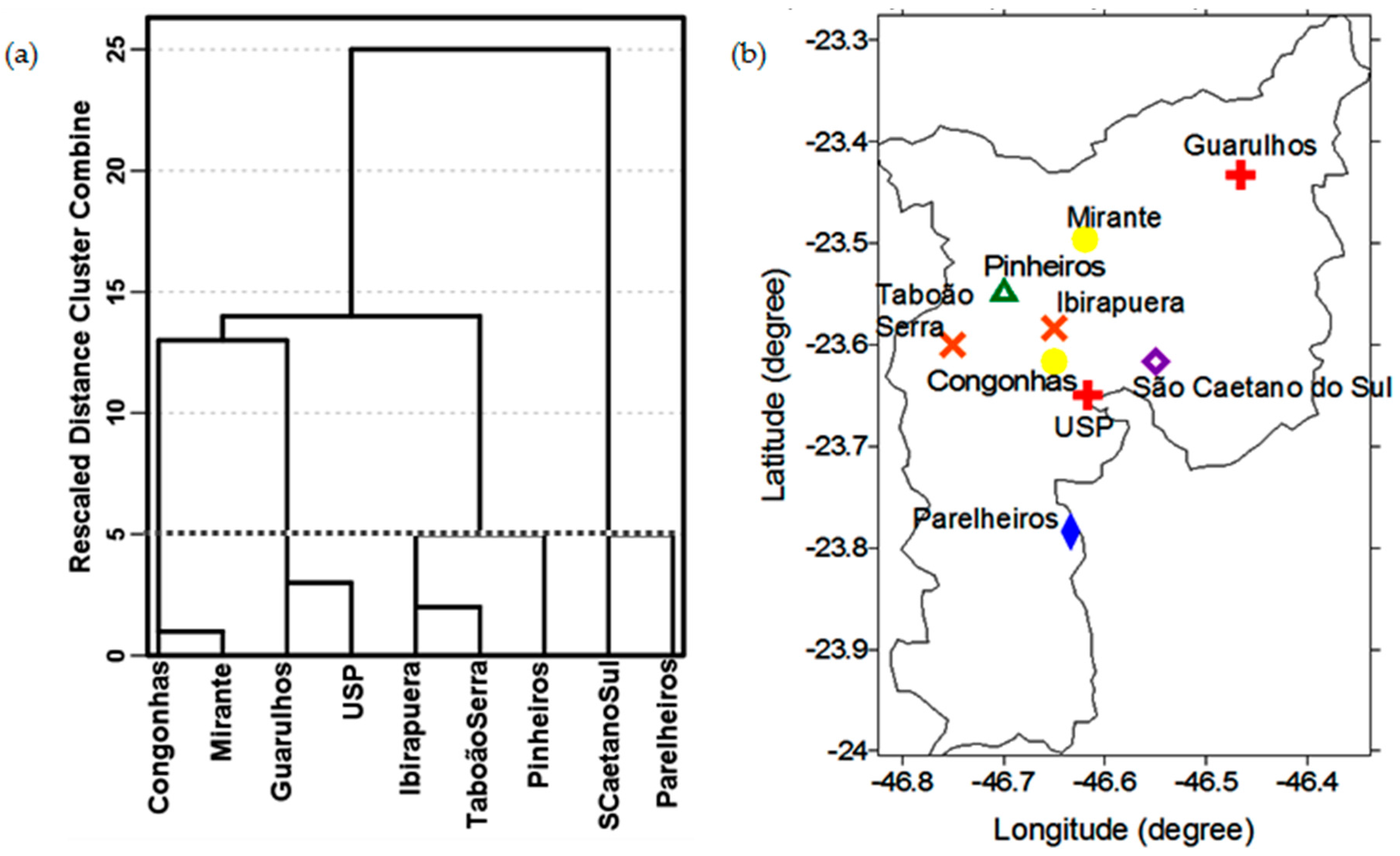
The threshold of six intra-homogeneous groups was the best representation of the MASP pattern and was consistent with the results we found with the EOF analysis. The six inner groups (Figure 18a) are group 1 (USP, Guarulhos), group 2 (Congonhas, Mirante), group 3 (Ibirapuera, Taboão Serra), group 4 (Pinheiros), group 5 (São Caetano do Sul), and group 6 (Parelheiros). Figure 18b illustrates the distribution map of the stations according to the six homogeneous groups in the MASP, and each color corresponds to a group. The spatial distribution of the groups (Figure 18b) indicates that the six homogeneous groups from the CA correspond to areas with spatial patterns found with the EOF analysis in both modes. Overall, the CA corroborates the EOF analysis, with the CA groups matching the spatial pattern of the second PC of the T-mode and the first PC of the S-mode.
A subjective analysis of the land-use classification map (Figure 5b) resulted in the identification of six groups, which we classified as follows: urban group 1 (São Caetano do Sul, purple), urban group 2 (Pinheiros, green), urban group 3 (Taboa Serra and Ibirapuera, orange), urban group 5 (Congonhas and Mirante, yellow), urban group 6 (Guarulhos and USP, red) and the vegetated group (Parelheiros, blue).
3.4. UHI Intensity
We used the average air temperature in each of the six homogeneous groups to determine the UHI intensity, being, therefore, a mean UHII. It should be emphasized that no filtering or removal of the influence of synoptic scale was carried out; also, no filtering or removal was carried out for days with a prevalence of weak winds, days with significant cloudiness, and even days corresponding to weekends and holidays.
Among the six groups identified with the CA, group 6 (composed of Parelheiros station only) stands out for being located in the region farthest from the central area of MASP and was predominantly characterized by scarce urbanization and more vegetated area. Therefore, to estimate the UHII, we chose group 6 to represent the temperature of non-urban/vegetated areas, and the other groups (1, 2, 3, 4 and 5) to represent the urban area.
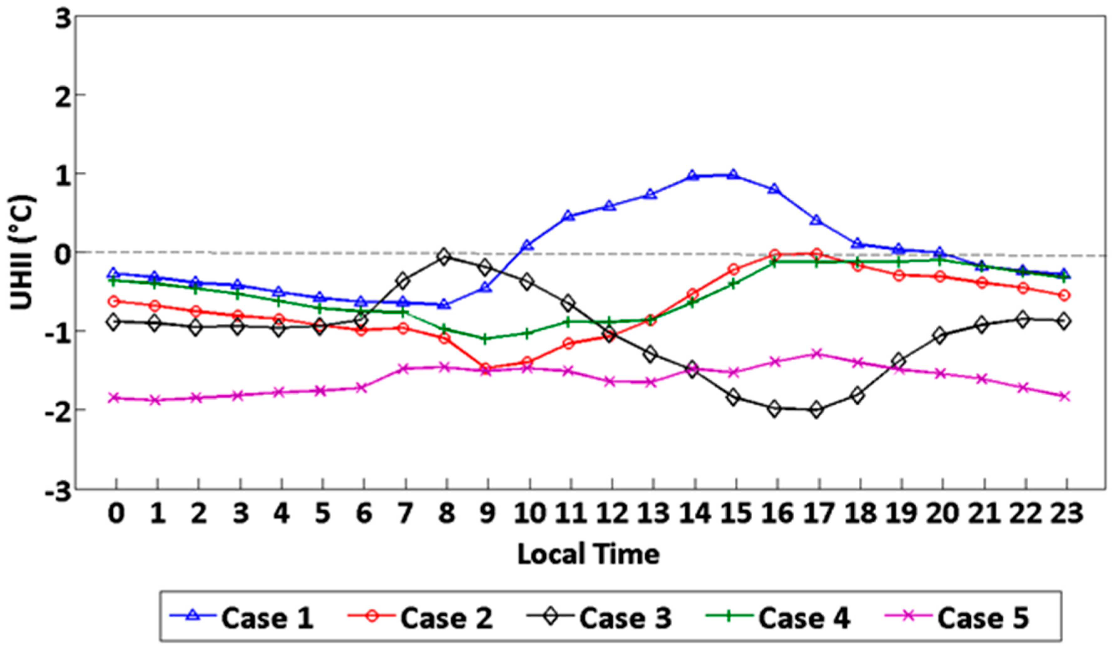
We estimated the UHII for each one of the urban groups considering the differences between the average temperature of each urban group and Parelheiros (group 6), which were then, respectively, denominated as case 1 to 5, after the group number. Except for case 5, we observed a clear diurnal cycle of the UHII, although each case peaks at different times (Figure 19).
For cases 1, 2 and 4, the UHII peaks in the afternoon, at approximately 15:00 LT for cases 1 and 2, and 17:00 LT for case 4. For case 3, a peak occurs in the morning at approximately 08:00 LT and a secondary peak occurs late in the evening at approximately 22:00 LT. The selection of reference stations reflects very distinct patterns of the UHII, therefore, specific criteria are recommended for their selection.
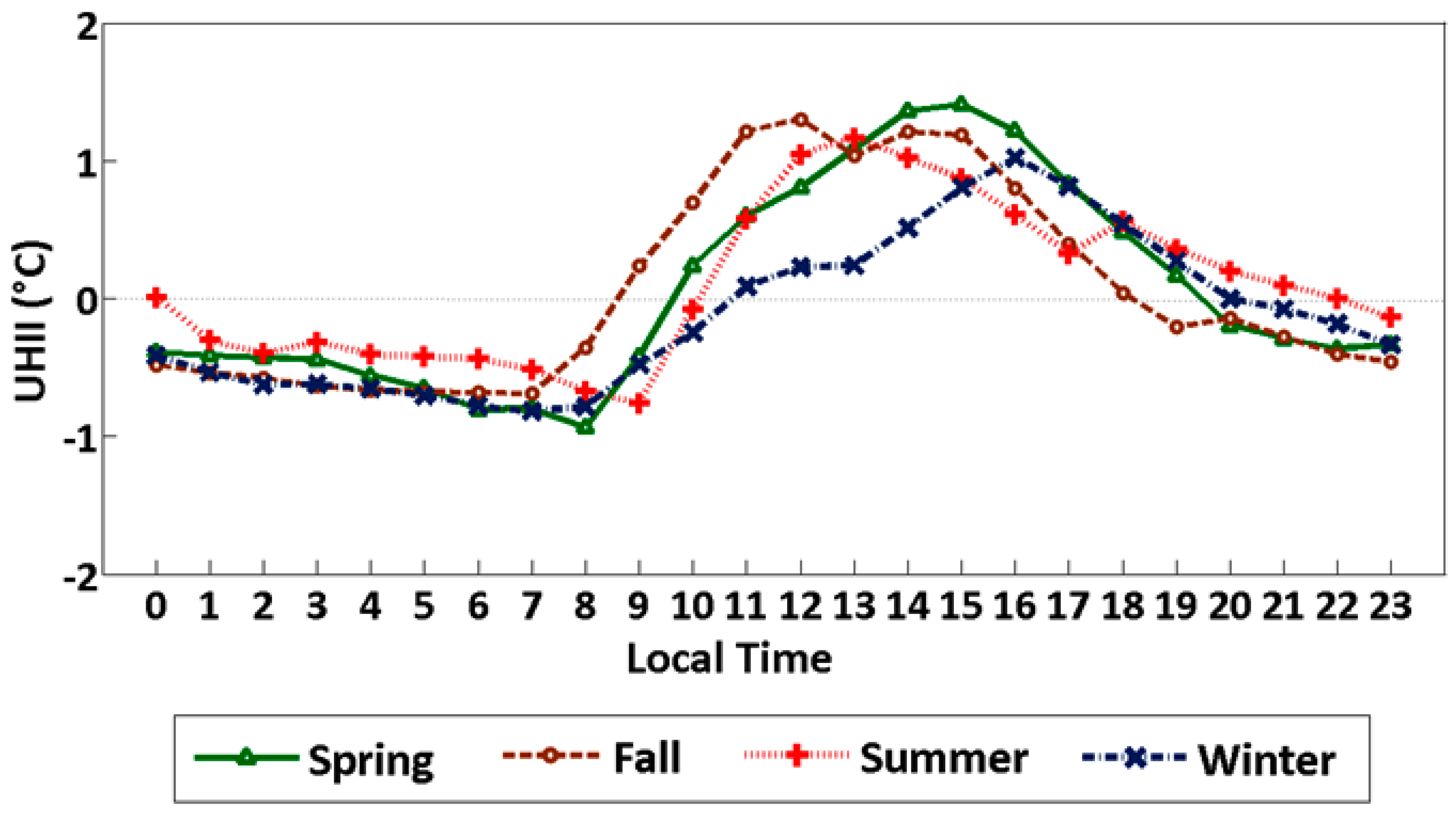
Among the UHII cases analyzed, case 1 is consistent with the pattern found by Ferreira et al. [30], who estimated the monthly UHI for 2004. The daytime behaviour of the UHII follows the diurnal evolution of net radiation at the surface for all months of the year, with a 3-h delay with the maximum intensity of net radiation. Therefore, we chose case 1 to assess the seasonal variability of the MASP UHI (Figure 20). Spring had the highest maximum and lowest minimum UHII values compared with the other seasons, and winter had the lowest UHII values. The maximum UHII occurred at different times for each season. In spring, summer and winter, the maximum UHII values occurred at 15:00 LT, 13:00 LT, and 16:00 LT, respectively. In autumn, there were two peaks, one at 12:00 LT and another between 14:00 and 15:00 LT. This variation is likely to be related to the incident solar radiation at the surface, which does have a significant seasonal variation. The shortwave radiation in São Paulo peaks during spring, particularly in September, and presents minimum values during fall and winter [30,55].
4. Conclusions
Multivariate analysis of observational temperature data demonstrated the spatial and temporal structures of the UHI in the MASP for the period from 2002 to 2011. In EOF analysis, both S- and T-modes allowed the recognition of dominant modes of variability of the UHI.
For the T-mode EOF, we identified three main modes of variability in the MASP, and they explained 99% of the total variance. The first mode explained 67% of the variance, the second mode explained 24%, and the third mode explained 8%. We associated the first and third modes of the EOF with the wind movement mechanisms of the MASP related to the sea breeze, whereas the second mode with the urbanization and the release of heat from the urban canopy and anthropogenic sources, as well as local wind circulation in the MASP. The spatial pattern of the temperature anomaly of the second PC is similar to the spatial distribution of the apparent surface temperature of the MASP.
For the S-mode EOF, we found only two modes of variability, and they accounted for 49% and 31% of the total variance. In the S-mode, the first mode represented the spatial pattern of the UHI in the MASP, and it was similar to the second mode of the T-mode EOF.
In the analysis of seasonal EOFs, we observed a difference in the number of variability modes, with summer and winter each presenting two modes, and fall and spring each presenting three modes. This difference is probably associated with the thermodynamic patterns of the atmosphere, which are different during each season, as well as due to remote influences, such as El Ninõ/La Ninã events, which can influence seasonal air temperatures in MASP.
Both forms of EOF analysis enabled the identification of the various warm core temperatures and their intensities, sizes, locations, and variations throughout the diurnal cycle. We identified six homogeneous groups with the CA, which were consistent with the core spatial patterns we found with the EOF analysis. Therefore, by applying multivariate analysis, we determined the main temperature anomaly patterns for the MASP.
In analysis of UHII, estimates of the temperature differences between the urban/suburban areas and the non-urban/vegetated areas were calculated. Group 6 (Parelheiros station) was regarded as the non-urban/vegetated group because it is located further from the central area of the MASP, and the other groups (1, 2, 3, 4 and 5) were regarded as the urban/suburban groups. The results of the UHII estimations showed that the maximum and minimum intensities of the UHI occurred at different hours for each case. Therefore, the selected reference stations may have reflected distinct UHII patterns, indicating what criteria should be adopted when selecting stations.
Detailed annual and seasonal analyses of the UHI for case 1 (temperature differences between the São Caetano do Sul and Parelheiros stations), demonstrated—in UHII annual analysis—a diurnal pattern with a maximum UHII between 14:00 and 16:00 LT and a minimum UHII between 07:00 and 09:00 LT. The daytime behavior of UHII found in the results agrees with the study of Ferreira et al. [30]; the maximum UHII value in the diurnal pattern occurred in the afternoon at approximately 3 h after the maximum intensity of net radiation. In UHII seasonal analysis, spring had the highest maximum and minimum UHI values. The maximum UHII in spring, particularly in September, is related to the maximum incident solar radiation caused by significant seasonal variations in atmospheric transmissivity and emissivity. In September, additional solar radiation reaches the surface and transmits a greater amount of longwave radiation.
The characterization of the air temperature field using multivariate analysis techniques (principal component analysis and cluster analysis) is an approach that is not well explored in urban climate studies. In this study, we demonstrated the robustness of this type of analyses, identifying the spatial and temporal patterns near the surface temperature in the urban area and surroundings of the MASP, which allowed us to assess and quantify the UHI phenomenon. Within the principal components, we recognized the primary physical patterns and mechanisms that act and influence the MASP, such as urbanization, local circulation, and the mutual influence between them that derives from other effects, such as urban breeze circulation. In the cluster analysis, the stations with similar characteristics are distributed in groups. The application of the multivariate analysis techniques highlights a new approach that could be further explored for urban studies to determine the intensity of UHI across regions and similar microclimatic zones.
In addition, this study evidenced another aspect not commonly discussed in urban studies. Although the UHI phenomenon is primarily established and dimensioned by the local characteristics of the urban area, the remote and local influences can also play a role in the seasonal behavior of air temperature, and thus in the UHI intensity. Our results highlight the importance of taking into account the remote and local influences in urban studies.
Acknowledgments
The authors would like to thank the National Council of Technological and Scientific Development (CNPq) for the financial support for this research. We also thank the CETESB, INEA, INMET, REDEMET and USP for providing access to their data.
Author Contributions
This paper is part of the first author Ph.D. thesis. The second and third authors are the advisor and a climate expert, respectively. Fernanda Batista Silva designed and carried out the research, gathering the data and applying the multivariate analysis. Karla Maria Longo de Freitas contributed with the data analysis and reviewed the work. Felipe Marques de Andrade contributed to the analysis of the relationship of remote and local influences with the local UHI phenomenon. All the authors reviewed and approved the final manuscript.
Conflicts of Interest
The authors declare no conflict of interest.
Appendix A
EOF Analysis
The EOF analysis aims to transform correlated original variables (K) to new uncorrelated or orthogonal (M) components/variables. These components are linear functions of the original components. Therefore, for vector × with multiple observations of (K × 1) data, the EOF generates a new vector u of (M × 1), which includes elements that are linear combinations of the elements of vector x and contain most of the information from the original vector. The elements of this new vector represent the maximum fraction of the variability in the original data and are called the principal components (PCs) [43].
Each PC generated by the EOF represents a portion of the variability in the dataset, and as the variance explained by the PC increases, the importance of PC in the representation of the dataset increases. The first mode or first PC is the linear combination of the original standardized variables, and it represents the fraction or percentage of the maximum variance. The second mode or second PC is the main component, or the linear combination of variables, which does not correlate with the first mode, and represents the largest proportion of the remaining variance. The subsequent principal components include linear combinations with the largest proportion of the remaining variance, and they are uncorrelated with principal components that have lower indices. The EOFs of each PC are mutually uncorrelated. Thus, the major advantage of using the EOF technique is that the classification of the eigenvectors associated with the largest eigenvalues of the correlation matrix allows the maximum variance to be explained [40].
The correlation matrix is written as follows:
where [Z]T is the transposed matrix of Z. The correlation matrix [R] is obtained by M eigenvalues λm (λ1 ≥ λ2 ≥ .... ≥ λk), and each of the eigenvalues corresponds to an eigenvector (:
Each eigenvector is one of the M components of the new orthogonal basis.
The new variables (PCs) are obtained projecting the original data on the new basis given by the eigenvectors of [R]:
Each of the M eigenvectors contains one element pertaining to each of the K variables and can be represented on a map that indicates the locations with the largest contributions to their main component and the simultaneous anomalies that are represented by this major component.
The EOF also provides the variance of the total analysis, which is defined by the sum of the variances of the observed variables as follows:
The value of the variance accounted for by each component is given by:
An important question regarding the EOF technique pertains to the number of eigenvalues that must be retained to differentiate between significant information and noise. To select the appropriate number of PCs for the analysis, the Kaiser truncation criterion is applied to retain the λm that meets the criterion:
where sk,k is the sample variance of the kth element and T is a threshold parameter. Kaiser’s criterion [54] uses Equation (6) with a threshold parameter T = 1 [43]. In this criterion, eigenvalues greater than one are considered the most significant.
The EOF rotated by the varimax orthogonal rotation method [56] was used to maximize the variance of the results. This method is a commonly used approach, and it is determined by choosing the elements of the rotation matrix to maximize as follows:
where n is the number of variables, r is the number of PCs, and bi are the eigenvectors. The rotated EOF has the advantage of producing new compact patterns that can be used for regionalization; thus, it divides the area into a limited number of homogeneous subareas [41]. The main objectives of rotated EOF analysis are to alleviate the strong constraints of the EOF (i.e., orthogonal/uncorrelated variables of PCs), to alleviate the dependence of the EOF pattern on the domain shape, and to obtain simple structures and easy interpretations of obtained patterns.
In the T-mode approach, the spatial fields (at a given time) of the variables used in analysis are considered the statistical variables. The domain is now temporal and the statistical observations are the different spatial points included in the instantaneous field [47]. Therefore, the T-mode not only identifies the main spatial patterns of the temperature anomaly field but also the order of occurrence.
To analyze the T-mode, a data matrix (n × m) was built, where n corresponds to the spatial field or “snapshot” of the mean hourly temperature anomalies (n = 9, which are weather stations of the MASP) and m corresponds to the statistical observations (m = 24, which are the mean hourly temperature anomalies of the 10 years of observations).
In the T-mode, the spatial patterns (PC scores) correspond to the principal types of temperature anomalies that describe the observed spatial variability, whereas the time series (PC loading) represents the correlation between the spatial patterns and each of the hourly mean anomaly fields. In the time series, the time at which a specific pattern occurs and the significance of its contribution to the real field at that time are observed. Therefore, when the time series shows low values (low PC loadings) for a specific time, the spatial pattern does not correspond to the structure of the temperature anomaly field. Thus, values closer to 1 in the time series represent sequences of weather conditions similar to the sequences of obtained patterns [48,49].
In the S-mode, the statistical variables are points in space, and the statistical observations are the observation times at which the variables are measured; thus, this mode can be used to study the behavior of the time series. The aim of the S-mode is to isolate the subsets of the spatial domain that have similar time variations and identify regions of similar behavior in time [50]. Therefore, although the characteristics of the field of study are not identified, the main features of the temporal variability of the field and the areas of influence of these modes are determined.
For S-mode analysis, a data matrix (n × m) was built, where n is the number of variables (n = 24, which is the mean hourly temperature anomalies of the 10 years of observations) and m corresponds to the number of observations (m = 9, which is the nine weather stations of the MASP).
In the S-mode approach, the time series (PC scores) correspond to the principal patterns of temporal variability for the temperature anomaly, and the spatial patterns (PC loadings) represent the correlation fields determined by the time series and all points in space. The spatial pattern field shows areas where the grid-point time series presents an in-level or anti-phase temporal behavior similar to that of the time series [50] such that low correlation values (low PC loadings) do not correspond to the behavior of the original observations for that particular mode.
T-mode and S-mode EOFs describe different aspects of the same real case. However, these two modes are supplementary and equally exclusive because their results cannot be reproduced by the mathematical manipulation of one another. In certain special cases, the S-mode and T-mode EOFs may produce results that are apparently similar, and a relationship might be observed between these “similarities” if there is an intrinsic and large linear spatial and temporal relationship that precludes any other effects, such as dispersion, which occurs over time because of the non-linearity of real systems [47,50].
Appendix B
Cluster Analysis
In Cluster analysis, the degree of similarity and difference between individual observations, x, is used to define the groups and to assign group membership. For a data vector sample x, which is defined by the (n × k) data of matrix [X], a classification scheme will define G groups and assign group memberships at varying levels of aggregation [43].
The CA fundamentally consists of a grouping function (called a distance or similarity measure) and a mathematical grouping criterion [51]. The composition of a cluster is based on the measured distances; thus, it is composed of points separated by small distances relative to the distances between clusters [43]. The similarity measure most commonly used in a CA is the Euclidean distance in the spatial dimension of the data vectors, and this approach was used here. A detailed discussion of various similarity measures can be found in [52]. The Euclidean distance between two vectors xi and xj is defined as follows:
After selecting a distance measure to quantify the dissimilarity or similarity between the pair of vectors xi and xj, the next step in CA is to choose a method or grouping criteria. The grouping processes can be divided into hierarchical or non-hierarchical processes, and hierarchical processes are more commonly used. The hierarchical clustering method is characterized by creating a set of groups in a hierarchy, each of which is formed by the integration of one pair from a collection of previously defined groups. The hierarchical method used in this study was Ward’s method [57], which is the most commonly used hierarchical method. In this method, the pair of groups to be merged minimizes the sum of the squared distances between the points and the centroids of their respective groups summed over the resulting groups. Thus, among all possible methods of merging two of the G + 1 groups to make G groups, the merge that minimizes W, is performed [43]:
This hierarchical search method for partitions minimizes the loss of information associated with each cluster [51]. One of the main advantages of the Ward method beyond its effectiveness in forming groups is that it tends to produce groups with the same number of elements.
The CA results are presented by a dendrogram or tree diagram, where the successive mergers of individuals into a single group are verified and the results are summarized. One of the difficulties of a CA is choosing how many clusters for analysis because an intermediate phase must be selected as the final solution. Thus, a level of clustering must be selected that minimizes the differences between the members of a given cluster and maximizes the differences between the members of different clusters [43]. There are no set criteria for the selection of clusters, although the process of interruption requires a subjective choice according to the goals of the analysis.
References
- Oke, T.R. The energetic basis of the urban heat island. Q. J. R. Meteorol. Soc. 1982, 108, 1–24. [Google Scholar] [CrossRef]
- Oke, T.R. Boundary Layer Climates, 2nd ed.; Routledge: London, UK, 1987. [Google Scholar]
- Arya, S.P. Introduction to Micrometeorology; Academic Press: San Diego, CA, USA, 2001; Volume 79. [Google Scholar]
- Arnfield, A.J. Two decades of urban climate research: A review of turbulence, exchanges of energy and water, and the urban heat island. Int. J. Climatol. 2003, 23, 1–26. [Google Scholar] [CrossRef]
- Kim, Y.; Baik, J. Spatial and temporal structure of the urban heat island in Seoul. J. Appl. Meteorol. 2005, 5, 591–605. [Google Scholar] [CrossRef]
- Sun, C.Y.; Brazel, A.J.; Chow, W.T.L.; Hedquist, B.C.; Prashad, L. Desert heat island study in winter by mobile transect and remote sensing techniques. Theor. Appl. Climatol. 2009, 98, 323–335. [Google Scholar] [CrossRef]
- Roth, M. Review of urban climate research in (sub) tropical regions. Int. J. Climatol. 2007, 27, 1859–1873. [Google Scholar] [CrossRef]
- Landsberg, H.E. The Urban Climate; Academic Press: New York, NY, USA, 1981; Volume 28. [Google Scholar]
- Oke, T.R.; Johnson, G.T.; Steyn, D.G.; Watson, I.D. Simulation of surface urban heat islands under “ideal” conditions at night. Part 2: Diagnosis of causation. Bound. Layer Meteorol. 1991, 56, 339–358. [Google Scholar] [CrossRef]
- Yoshikado, H. High levels of winter air pollution under the influence of the urban heat island along the shore of Tokyo Bay. J. Appl. Meteorol. 1996, 35, 1804–1813. [Google Scholar] [CrossRef]
- Taha, H. Urban climates and heat islands: Albedo, evapotranspiration, and anthropogenic heat. Energy Build. 1997, 25, 99–103. [Google Scholar] [CrossRef]
- Grimmond, C.S.B. Progress in measuring and observing the urban atmosphere. Theor. Appl. Climatol. 2006, 84, 3–22. [Google Scholar] [CrossRef]
- Rosenzweig, C.; Solecki, W.; Slosberg, R. Mitigating New York City’s Heat Island with Urban Forestry, Living Roofs, and Light Surfaces; A Report to the New York State Energy Research and Development Authority; American Meteorological Society: Boston, MA, USA, 2006. [Google Scholar]
- Sarrat, C.; Lemonsu, A.; Masson, V.; Guedalia, D. Impact of urban heat island on regional atmospheric pollution. Atmos. Environ. 2006, 40, 1743–1758. [Google Scholar] [CrossRef]
- Rizwan, A.M.; Dennis, L.; Liu, C. A review on the generation, determination and mitigation of Urban Heat Island. J. Environ. Sci. 2008, 20, 120–128. [Google Scholar] [CrossRef]
- Hidalgo, J.; Masson, V.; Baklanov, A.; Pigeon, G.; Gimeno, L. Advances in urban climate modeling. Ann. N. Y. Acad. Sci. 2008, 1146, 354–374. [Google Scholar] [CrossRef] [PubMed]
- Onishi, A.; Cao, X.; Ito, T.; Shi, F.; Imura, H. Evaluating the potential for urban heat-island mitigation by greening parking lots. Urban For. Urban Green. 2010, 9, 323–332. [Google Scholar] [CrossRef]
- Sailor, D.J. A review of methods for estimating anthropogenic heat and moisture emissions in the urban environment. Int. J. Climatol. 2011, 31, 189–199. [Google Scholar] [CrossRef]
- Kolokotroni, M.; Ren, X.; Davies, M.; Mavroganni, A. London’s urban heat island: Impact on current and future energy consumption in office buildings. Energy Build. 2012, 47, 302–311. [Google Scholar] [CrossRef]
- Montávez, J.P.; Rodríguez, A.; Jiménez, J.I. A Study of the Urban Heat Island of Granada. Int. J. Climatol. 2000, 20, 899–911. [Google Scholar] [CrossRef]
- Oliveira, A.P.; Bornstein, R.D.; Soares, J. Annual and diurnal wind patterns in the city of São Paulo. Water Air Soil Pollut. Focus 2003, 3, 3–15. [Google Scholar] [CrossRef]
- Fujibe, F. Detection of urban warming in recent temperature trends in Japan. Int. J. Climatol. 2009, 29, 1811–1822. [Google Scholar] [CrossRef]
- Hicks, B.B.; Callahan, W.J.; Hoekzema, M.A. On the Heat Islands of Washington, DC, and New York City, NY. Bound. Layer Meteorol. 2010, 135, 291–300. [Google Scholar] [CrossRef]
- Murphy, D.J.; Hall, M.H.; Hall, C.A.; Heisler, G.M.; Stehman, S.V.; Anselmi-Molina, C. The relationship between land cover and the urban heat island in northeastern Puerto Rico. Int. J. Climatol. 2011, 31, 1222–1239. [Google Scholar] [CrossRef]
- Camilloni, I.; Barrucand, M. Temporal variability of the Buenos Aires, Argentina, urban heat island. Int. J. Climatol. 2011, 31, 1222–1239. [Google Scholar] [CrossRef]
- Ozdemir, H.; Unal, A.; Kindap, T.; Turuncoglu, U.U.; Demir, G.; Tayanc, M.; Karaca, M. Quantification of the urban heat island under a changing climate over Anatolian Peninsula. Theor. Appl. Climatol. 2012, 108, 31–38. [Google Scholar] [CrossRef]
- Pereira Filho, A.J. Summer convection in urban environments and the flash floods. An. Acad. Bras. Ciênc. 2000, 72, 289–290. [Google Scholar] [CrossRef]
- Freitas, E.D. Circulações Locais em São Paulo e Sua Influência Sobre a Dispersão de Poluentes. Ph.D. Thesis, Department of Atmospheric Sciences, University of São Paulo, São Paulo, Brazil, 2003; p. 165. Available online: http://www.teses.usp.br/teses/disponiveis/14/14133/tde-16032006–160700/pt-br.php (accessed on 18 January 2017).
- Freitas, E.D.; Rozoff, C.; Cotton, W.R.; Silva Dias, P.L. Interactions of urban heat island and sea breeze circulations during winter over The Metropolitan Area of São Paulo—Brazil. Bound.-Layer Meteorol. 2007, 122, 43–65. [Google Scholar] [CrossRef]
- Ferreira, M.J.; de Oliveira, A.P.; Soares, J.; Codato, G.; Bárbaro, E.W.; Escobedo, J.F. Radiation balance at the surface in the city of São Paulo, Brazil: Diurnal and seasonal variations. Theor. Appl. Climatol. 2012, 107, 229–246. [Google Scholar] [CrossRef]
- Monteiro, C.A.F. Some aspects of the urban climates of tropical South America: The Brazilian contribution. In Urban Climatology and Its Applications with Special Regard to Tropical Areas; WMO No. 652; Oke, T.R., Ed.; World Meteorological Organization: Geneva, Switzerland, 1986; pp. 166–198. [Google Scholar]
- Gonçalves, F.L.T.; Silva Dias, P.L.; Araújo, G.P. Climatological analysis of wintertime extreme low temperatures in São Paulo City, Brazil: Impact of sea-surface temperature anomalies. Int. J. Climatol. 2002, 22, 1511–1526. [Google Scholar] [CrossRef]
- Ferreira, M.J.; de Oliveira, A.P.; Soares, J. Anthropogenic heat in the city of São Paulo, Brazil. Theor. Appl. Climatol. 2011, 104, 43–56. [Google Scholar] [CrossRef]
- Ogashawara, I.; Bastos, V.D.S.B. A quantitative approach for analyzing the relationship between urban heat islands and land cover. Remote Sens. 2012, 4, 3596–3618. [Google Scholar]
- Johansson, E.; Spangenberg, J.; Gouvêa, M.L.; Freitas, E.D. Scale-integrated atmospheric simulations to assess thermal comfort in different urban tissues in the warm humid summer of São Paulo, Brazil. Urban Clim. 2013, 6, 24–43. [Google Scholar] [CrossRef]
- Araujo, R.V.; Albertini, M.R.; Costa-da-Silva, A.L.; Suesdek, L.; Franceschi, N.C.; Bastos, N.M.; Katz, G.; Cardoso, V.A.; Castro, B.C.; Capurro, M.L.; et al. São Paulo urban heat islands have a higher incidence of dengue than other urban areas. Braz. J. Infect. Dis. 2015, 19, 146–155. [Google Scholar] [CrossRef] [PubMed]
- SVMA—Municipal Secretariat for Environment, Environmental Atlas of São Paulo, São Paulo City Hall. Available online: http://atlasambiental.prefeitura.sp.gov.br/mapas/105.pdf (accessed on 3 March 2017).
- NASA LP DAAC, 2010, Combined MODIS—Land Cover Type Yearly L3 Global 500 m SIN Grid (MCD12Q1). Version 5.1. NASA EOSDIS Land Processes DAAC, USGS Earth Resources Observation and Science (EROS) Center: Sioux Falls, South Dakota. Available online: http://dx.doi.org/10.5067/modis/modis_products_table/MCD12Q1 (accessed on 3 March 2017).
- Simmons, A.J.; Poli, P.; Dee, D.P.; Berrisford, P.; Hersbach, H.; Kobayashi, S.; Peubey, C. Estimating low-frequency variability and trends in atmospheric temperature using ERA-Interim. Q. J. R. Meteorol. Soc. 2014, 140, 329–353. [Google Scholar] [CrossRef]
- Preisendorfer, R.W. Principal Component Analysis in Meteorology and Oceanography; Mobley, C.D., Ed.; Elsevier: Amsterdam, The Netherlands, 1988. [Google Scholar]
- Hannachi, A.; Jolliffe, I.T.; Stephenson, D.B. Empirical orthogonal functions and related techniques in atmospheric science: A review. Int. J. Climatol. 2007, 27, 1119–1152. [Google Scholar] [CrossRef]
- Lorenz, E.N. Empirical Orthogonal Functions and Statistical Weather Prediction; Scientific Report No. 1, Statistical Forecasting Project; Massachusetts Institute of Technology: Cambridge, MA, USA, 1956. [Google Scholar]
- Wilks, D.S. Statistical Methods in the Atmospheric Sciences; Academic Press: Amsterdam, The Netherlands, 2006; Volume 100. [Google Scholar]
- Cattell, R.B. Factor Analysis; Harper and Row: New York, NY, USA, 1952. [Google Scholar]
- Green, P. Analyzing Multivariate Data; The Dryden Press: Oak Brook, IL, USA, 1978. [Google Scholar]
- Richman, M. Rotation of Principal Components. J. Climatol. 1986, 6, 293–335. [Google Scholar] [CrossRef]
- Salles, M.A.; Canziani, P.O.; Compagnucci, R.H. The spatial and temporal behaviour of the lower stratospheric temperature over the Southern Hemisphere: The MSU view. Part II: Spatial behaviour. Int. J. Climatol. 2001, 21, 439–454. [Google Scholar] [CrossRef]
- Harman, H. Modern Factor Analysis; The University of Chicago Press: Chicago, IL, USA, 1976. [Google Scholar]
- Cattell, R.B. The Scientific Use of Factor Analysis: In Behavioral and Life Sciences; Plenum Press: New York, NY, USA; London, UK, 1978. [Google Scholar]
- Compagnucci, R.H.; Salles, M.A.; Canziani, P.O. The spatial and temporal behaviour of the lower stratospheric temperature over the Southern Hemisphere: The MSU view. Part I: Data, methodology and temporal behaviour. Int. J. Climato. 2001, 21, 419–437. [Google Scholar] [CrossRef]
- Everitt, B.S. Cluster Analysis. In Heinemann Educational Books; Academic Press: London, UK, 1993. [Google Scholar]
- Duran, B.S.; Odell, P.L. Cluster Analysis: A Survey; Volume 100 of Lecture Notes in Economics and Mathematical Systems; Springer: Berlin/Heidelberg, Germany, 1974. [Google Scholar]
- Memon, R.A.; Leung, D.Y.; Liu, C.H. An investigation of urban heat island intensity (UHII) as an indicator of urban heating. Atmos. Res. 2009, 94, 491–500. [Google Scholar] [CrossRef]
- Grimm, A.M.; Ambrizzi, T. Teleconnections into South America from the tropics and extratropics on interannual and intraseasonal timescales. In Past Climate Variability in South America and Surrounding Regions; Springer: Dordrecht, The Netherland, 2009; pp. 159–191. [Google Scholar]
- Oliveira, A.P.; Escobedo, J.F.; Machado, A.J.; Soares, J. Diurnal evolution of solar radiation at the surface in the City of São Paulo. Seasonal variation and modeling. Theor. Appl. Climatol. 2002, 71, 231–249. [Google Scholar] [CrossRef]
- Kaiser, H.F. The varimax criterion for analytic rotation in factor analysis. Psychometrika 1958, 23, 187–200. [Google Scholar] [CrossRef]
- Ward, J.H. Hierarchical grouping of otimize an objetive function. J. Am. Stat. Assoc. 1963, 58, 236–244. [Google Scholar] [CrossRef]
Figure 1.
(a) Geographical location of the metropolitan area of São Paulo (MASP) in Brazil; (b) magnified views of the MASP.
Figure 1.
(a) Geographical location of the metropolitan area of São Paulo (MASP) in Brazil; (b) magnified views of the MASP.

Figure 2.
Three-dimensional view of the MASP, including the Mantiqueira and Serra do Mar Mountains and part of the Paulista Coast. The altitude of Mantiqueira and Serra do Mar Mountains near to MASP range between 900 and 1200 m and 400 and 700 m above the sea level (asl), respectively; while the MASP altitudes are between 700 and 800 m asl.
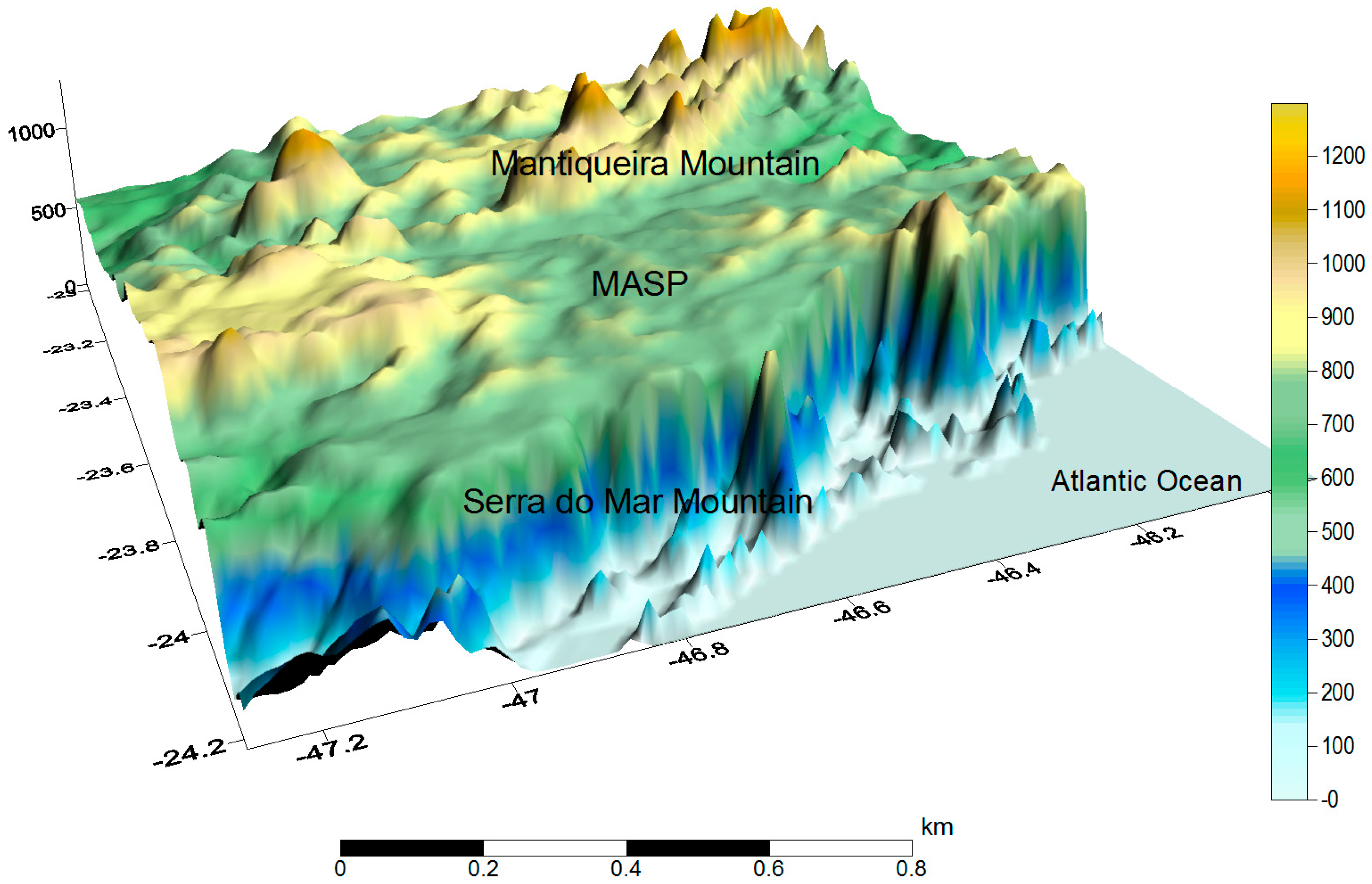
Figure 3.
Present land use of the MASP. The color scale indicates the urban area (red), and the predominant types of land covers MASP [38].
Figure 3.
Present land use of the MASP. The color scale indicates the urban area (red), and the predominant types of land covers MASP [38].

Figure 4.
Map of the apparent surface temperature in MASP on 3 September 1999, 09:57 local time (LT) inferred by the satellite Landsat-7 [37].
Figure 4.
Map of the apparent surface temperature in MASP on 3 September 1999, 09:57 local time (LT) inferred by the satellite Landsat-7 [37].

Figure 5.
(a) Map of the MASP with the following weather station locations: (1) Ibirapuera Park; (2) Congonhas Airport; (3) Taboão da Serra; (4) Pinheiros; (5) Mirante de Santana; (6) Guarulhos Airport; (7) São Caetano do Sul; (8) Água Funda; and (9) Parelheiros. The dark grey area highlights the new delimitation of the maps, which demarcates the effective area used in this study; (b) MASP station locations shown over a land-use satellite image. The same color scale depicted in Figure 3 is valid here [38].
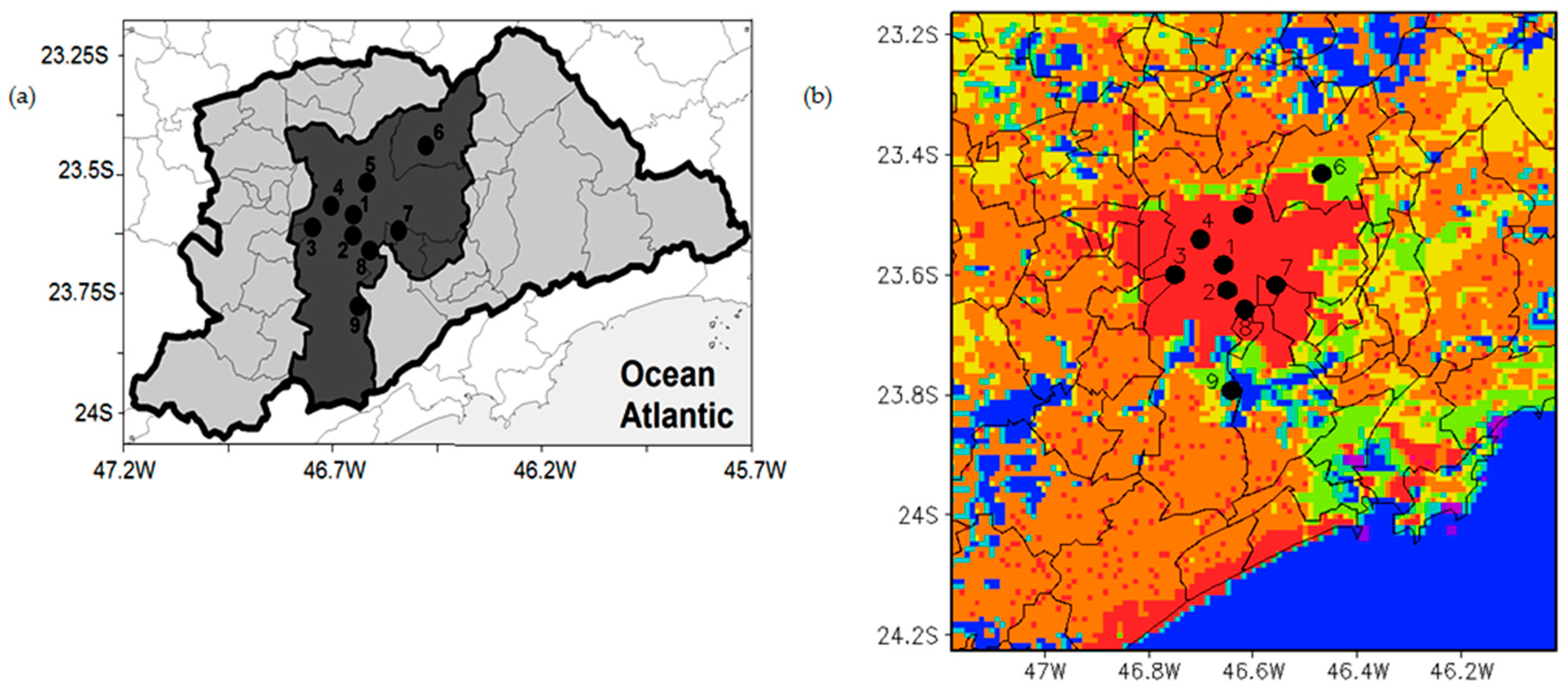
Figure 6.
Annual cycle of temperature near the surface (blue bars), and solar radiation (red line) averaged over the 10-year period from January 2002 to December 2011 in the MASP.
Figure 6.
Annual cycle of temperature near the surface (blue bars), and solar radiation (red line) averaged over the 10-year period from January 2002 to December 2011 in the MASP.
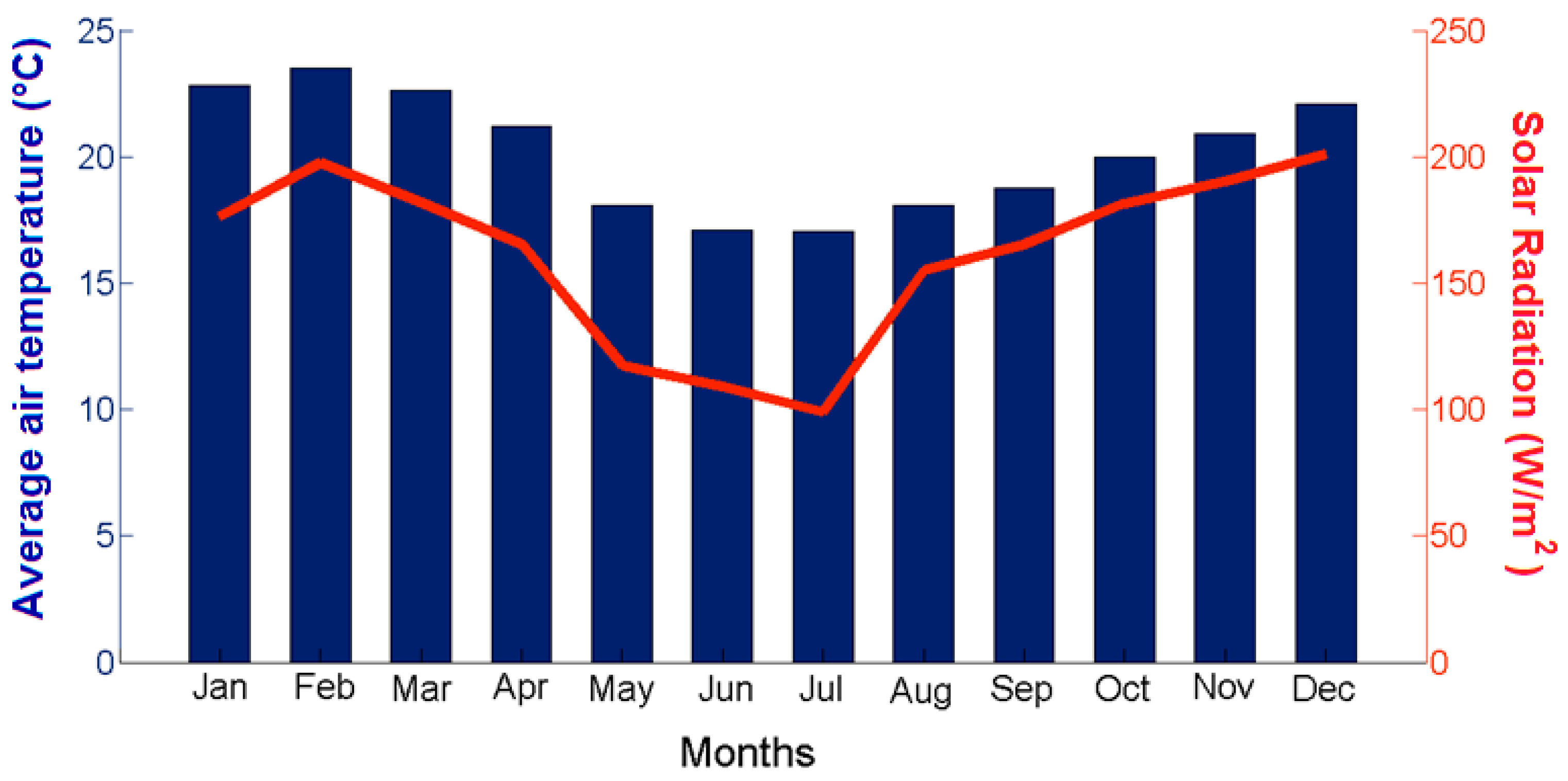
Figure 7.
Diurnal cycle of air temperatures averaged over the period from January 2002 to December 2011 in the MASP.
Figure 7.
Diurnal cycle of air temperatures averaged over the period from January 2002 to December 2011 in the MASP.

Figure 8.
Mean compass rose (direction and intensity) measurements at stations in the MASP for the period from 2002 to 2011.
Figure 8.
Mean compass rose (direction and intensity) measurements at stations in the MASP for the period from 2002 to 2011.
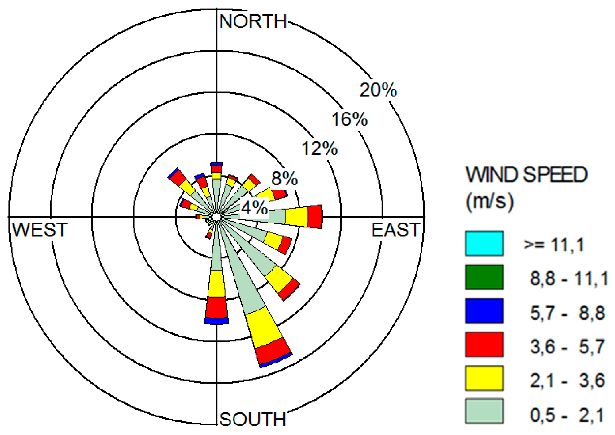
Figure 9.
Principal components (PC) loading time series of the first (67%), second (24%) and third (8%) T-mode empirical orthogonal functions (EOFs) calculated using the hourly mean temperature anomaly data for the MASP from January 2002 to December 2011.
Figure 9.
Principal components (PC) loading time series of the first (67%), second (24%) and third (8%) T-mode empirical orthogonal functions (EOFs) calculated using the hourly mean temperature anomaly data for the MASP from January 2002 to December 2011.

Figure 10.
PC score spatial pattern of the (a) first (67%); (b) second (24%) and (c) third (8%) T-mode EOFs calculated using the hourly mean temperature anomaly data of the MASP from January 2002 to December 2011. The thicker black line represents zero value. Isolines are on 0.2 intervals.
Figure 10.
PC score spatial pattern of the (a) first (67%); (b) second (24%) and (c) third (8%) T-mode EOFs calculated using the hourly mean temperature anomaly data of the MASP from January 2002 to December 2011. The thicker black line represents zero value. Isolines are on 0.2 intervals.

Figure 11.
PC score time series of the first (49%) and second (31%) S-mode EOFs calculated using the hourly mean temperature anomaly data of the MASP from January 2002 to December 2011.
Figure 11.
PC score time series of the first (49%) and second (31%) S-mode EOFs calculated using the hourly mean temperature anomaly data of the MASP from January 2002 to December 2011.
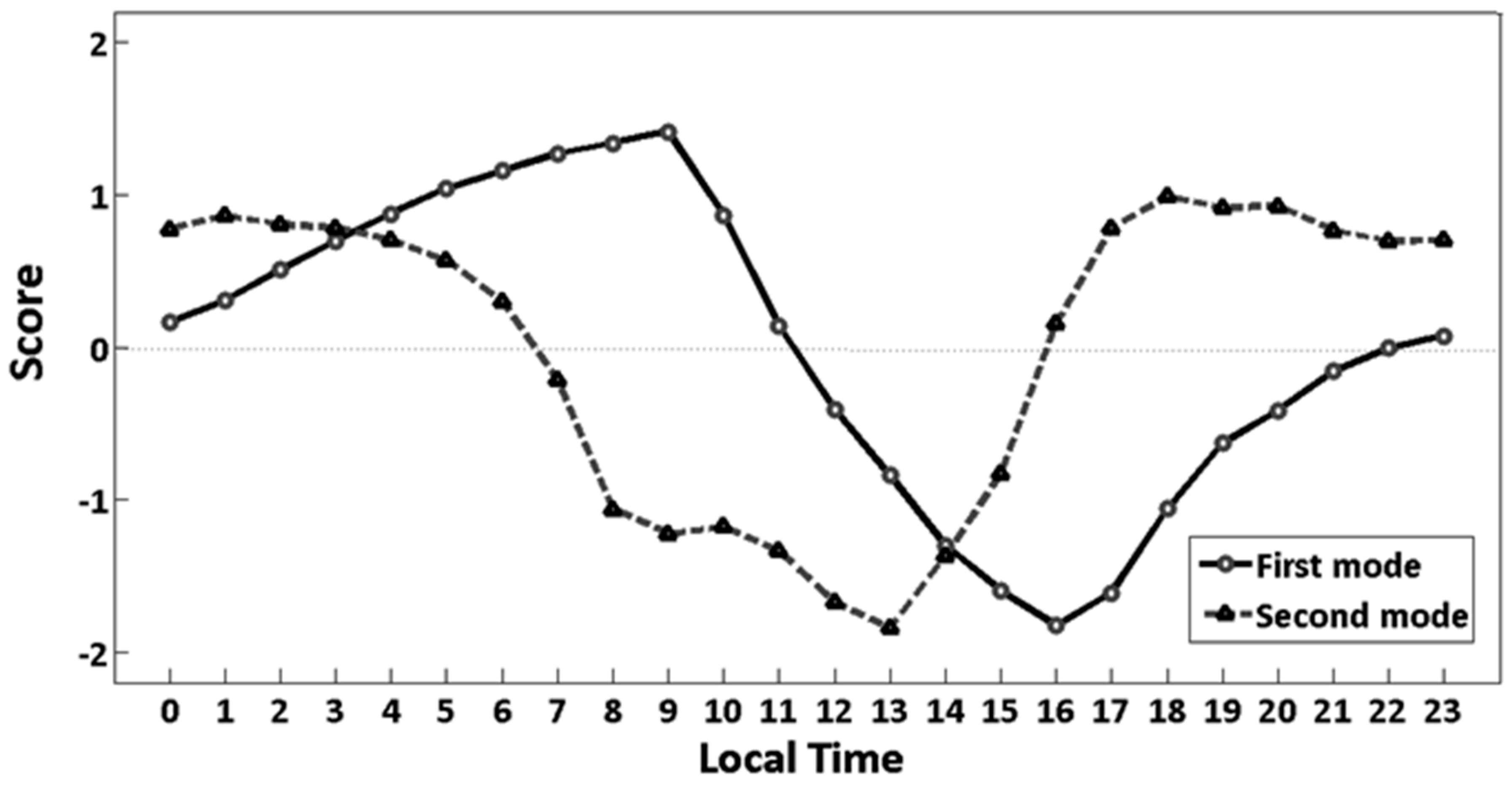
Figure 12.
PC loading spatial pattern of the (a) first (49%) and (b) second (31%) S-mode EOFs calculated using the hourly mean temperature anomaly data of the MASP from January 2002 to December 2011. The thicker black line represents zero value. Isolines are on 0.2 intervals.
Figure 12.
PC loading spatial pattern of the (a) first (49%) and (b) second (31%) S-mode EOFs calculated using the hourly mean temperature anomaly data of the MASP from January 2002 to December 2011. The thicker black line represents zero value. Isolines are on 0.2 intervals.
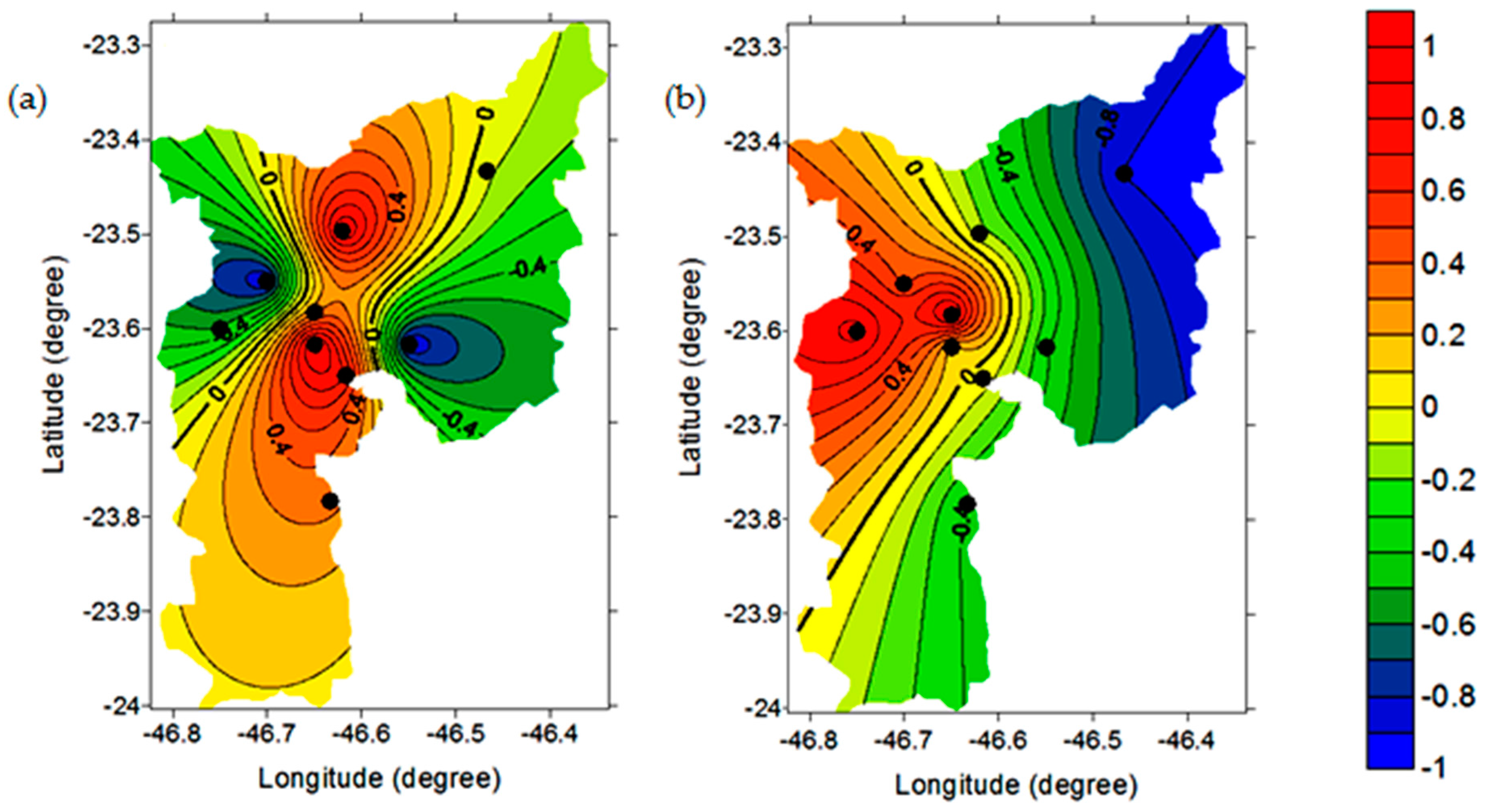
Figure 13.
PC score spatial patterns of the (a) first (78%) and (b) second (17%) T-mode EOFs in summer and the patterns in the (c) first (75%) and (d) second (20%) T-mode EOFs in winter; these patterns were calculated using the hourly mean temperature anomaly data of the MASP from January 2002 to December 2011. The thicker black line represents zero value. Isolines are on 0.2 intervals.
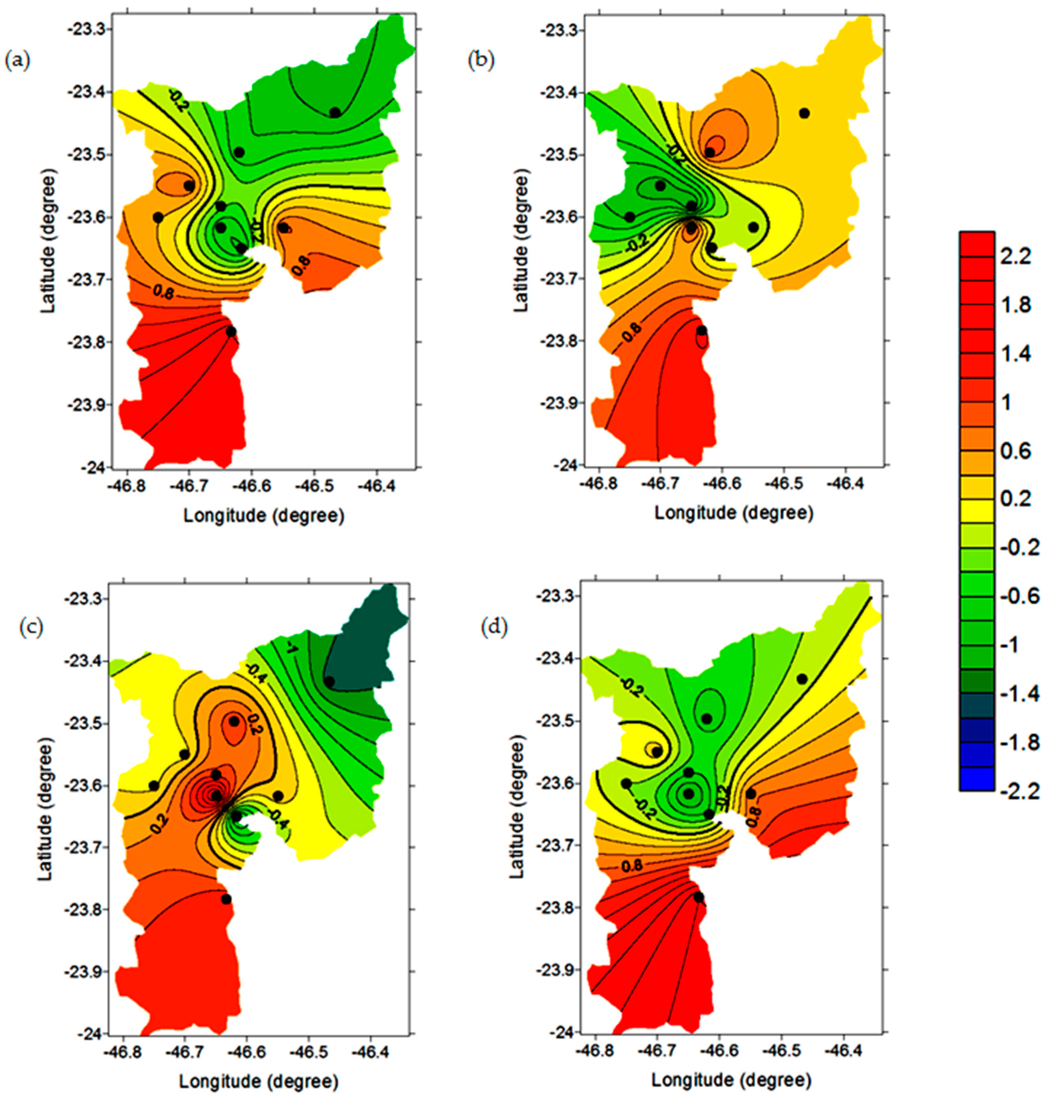
Figure 14.
PC loading time series of the first and second T-mode EOFs during (a) summer and (b) winter, which were calculated using hourly mean temperature anomaly data of the MASP from January 2002 to December 2011.
Figure 14.
PC loading time series of the first and second T-mode EOFs during (a) summer and (b) winter, which were calculated using hourly mean temperature anomaly data of the MASP from January 2002 to December 2011.

Figure 15.
PC score spatial pattern of the (a) first (69%); (b) second (23%) and (c) third (6%) T-mode EOFs during fall and the pattern in the (d) first (55%); (e) second (28%) and (f) third (14%) T-mode EOFs during spring; these patterns were calculated using the hourly mean temperature anomaly data of the MASP from January 2002 to December 2011. The thicker black line represents zero value. Isolines are on 0.2 intervals.
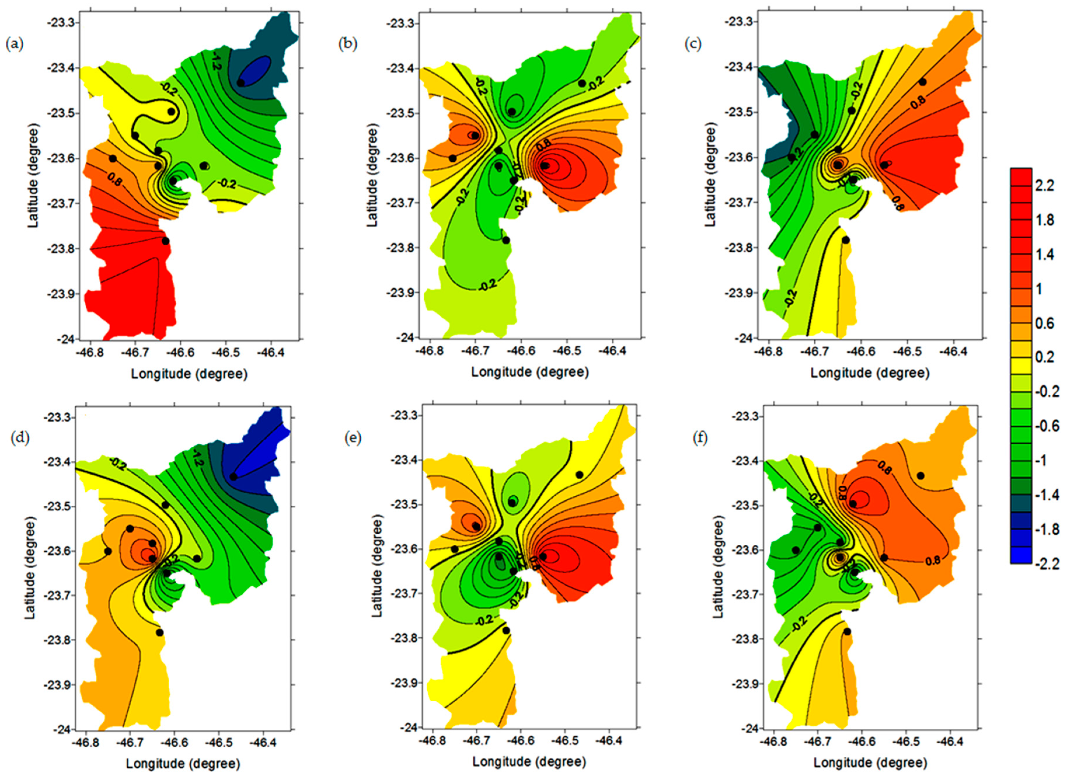
Figure 16.
PC loading time series of the first and second T-mode EOFs during (a) fall and (b) spring, which were calculated using hourly mean temperature anomaly data of the MASP from January 2002 to December 2011.
Figure 16.
PC loading time series of the first and second T-mode EOFs during (a) fall and (b) spring, which were calculated using hourly mean temperature anomaly data of the MASP from January 2002 to December 2011.
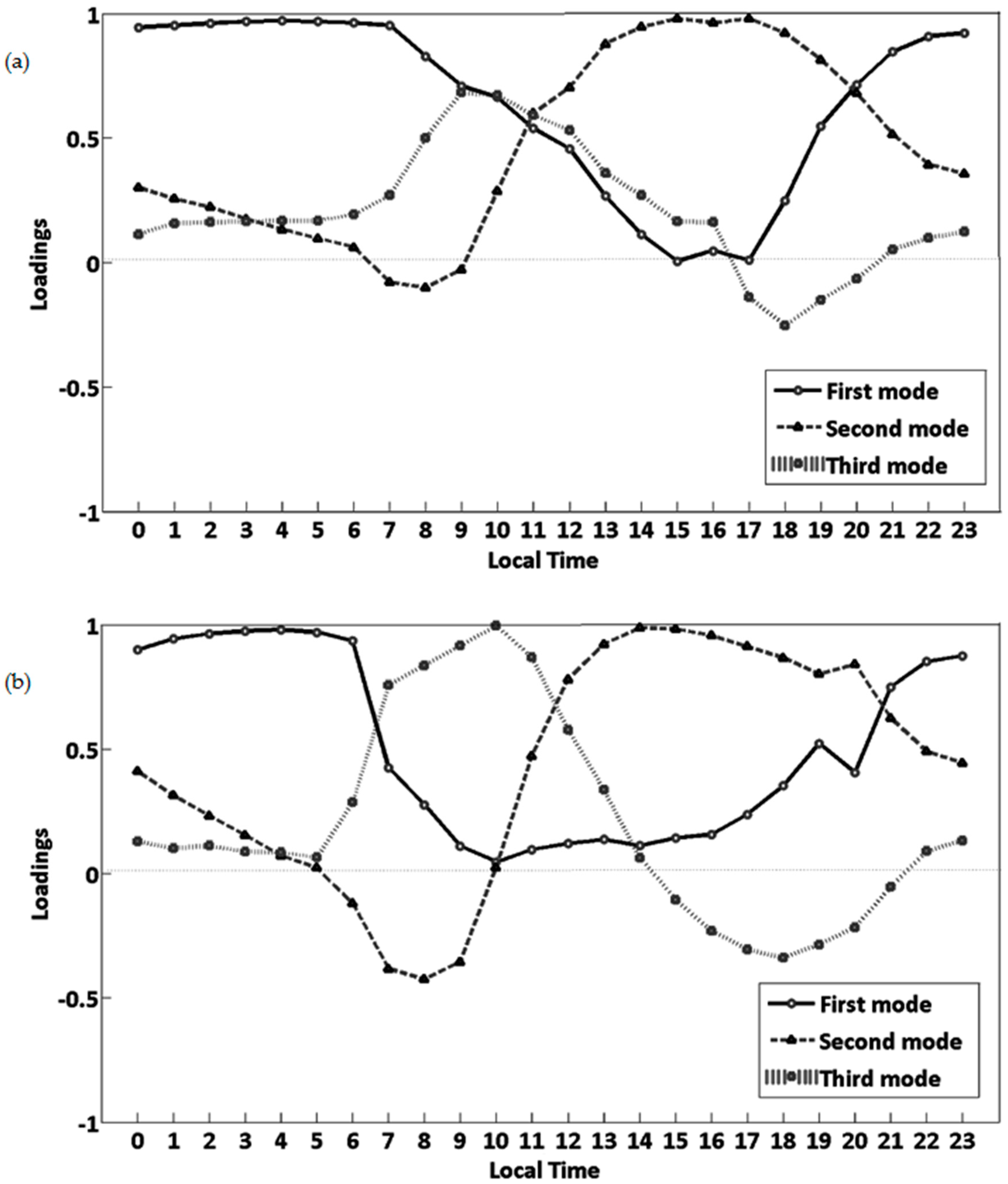
Figure 17.
Distribution of the correlation coefficients between the sea surface temperature (SST) anomaly data and mean temperature anomaly data in the MASP at the 95% significance level (Student’s t-test): (a) summer; (b) fall; (c) winter and (d) spring. The regions with positive (negative) correlation are solid (dashed) isolines and the first value is 0.55 (−0.55). Isolines are on 0.1 intervals. Oceanic areas of the South Atlantic along the southeastern region of Brazil and Equatorial Pacific corresponding area of the Niño 3.4 are delimited in square.

Figure 18.
(a) The resulting dendrogram for nine weather stations and (b) the distribution map of the stations within six homogeneous groups in the MASP. Each symbol (or colour) corresponds to a group: ![Environments 04 00027 i001]() (red—group 1);
(red—group 1); ![Environments 04 00027 i002]() (yellow—group 2);
(yellow—group 2); ![Environments 04 00027 i003]() (orange—group 3);
(orange—group 3); ![Environments 04 00027 i004]() (green—group 4);
(green—group 4); ![Environments 04 00027 i005]() (purple—group 5) and
(purple—group 5) and ![Environments 04 00027 i006]() (blue—group 6).
(blue—group 6).
 (red—group 1);
  (yellow—group 2);
  (orange—group 3);
  (green—group 4);
  (purple—group 5) and
  (blue—group 6).
Figure 18.
(a) The resulting dendrogram for nine weather stations and (b) the distribution map of the stations within six homogeneous groups in the MASP. Each symbol (or colour) corresponds to a group: ![Environments 04 00027 i001]() (red—group 1);
(red—group 1); ![Environments 04 00027 i002]() (yellow—group 2);
(yellow—group 2); ![Environments 04 00027 i003]() (orange—group 3);
(orange—group 3); ![Environments 04 00027 i004]() (green—group 4);
(green—group 4); ![Environments 04 00027 i005]() (purple—group 5) and
(purple—group 5) and ![Environments 04 00027 i006]() (blue—group 6).
(blue—group 6).
(red—group 1); (yellow—group 2); (orange—group 3); (green—group 4); (purple—group 5) and (blue—group 6).
Figure 19.
Annual mean diurnal cycle of the urban heat island (UHI) intensity for the different cases: case 1 (São Caetano do Sul—Parelheiros), case 2 (Pinheiros—Parelheiros), case 3 (Congonhas/Mirante—Parelheiros), case 4 (Ibirapuera/Taboão da Serra—Parelheiros), and case 5 (Guarulhos/USP—Parelheiros).

Figure 20.
Seasonal diurnal cycle of UHI intensity in the MASP for case 1: spring (green), fall (brown), summer (red) and winter (blue).
Figure 20.
Seasonal diurnal cycle of UHI intensity in the MASP for case 1: spring (green), fall (brown), summer (red) and winter (blue).

© 2017 by the authors. Licensee MDPI, Basel, Switzerland. This article is an open access article distributed under the terms and conditions of the Creative Commons Attribution (CC BY) license (http://creativecommons.org/licenses/by/4.0/).
Share and Cite
MDPI and ACS Style
Silva, F.B.; Longo, K.M.; De Andrade, F.M. Spatial and Temporal Variability Patterns of the Urban Heat Island in São Paulo. Environments 2017, 4, 27. https://doi.org/10.3390/environments4020027
AMA Style
Silva FB, Longo KM, De Andrade FM. Spatial and Temporal Variability Patterns of the Urban Heat Island in São Paulo. Environments. 2017; 4(2):27. https://doi.org/10.3390/environments4020027
Chicago/Turabian StyleSilva, Fernanda Batista, Karla Maria Longo, and Felipe Marques De Andrade. 2017. "Spatial and Temporal Variability Patterns of the Urban Heat Island in São Paulo" Environments 4, no. 2: 27. https://doi.org/10.3390/environments4020027
Note that from the first issue of 2016, this journal uses article numbers instead of page numbers. See further details here.