
Estimating the Probability of Vegetation to Be Groundwater Dependent Based on the Evaluation of Tree Models


Abstract
:
1. Introduction
- Ecosystems dependent on the surface expression of groundwater: this category includes springs, “minerogenous” wetlands (wetlands supported by groundwater that has been in contact with mineral soils or bedrock), river baseflow systems, and some estuarine and near-shore marine ecosystems that depend on the near-shore discharge of groundwater.
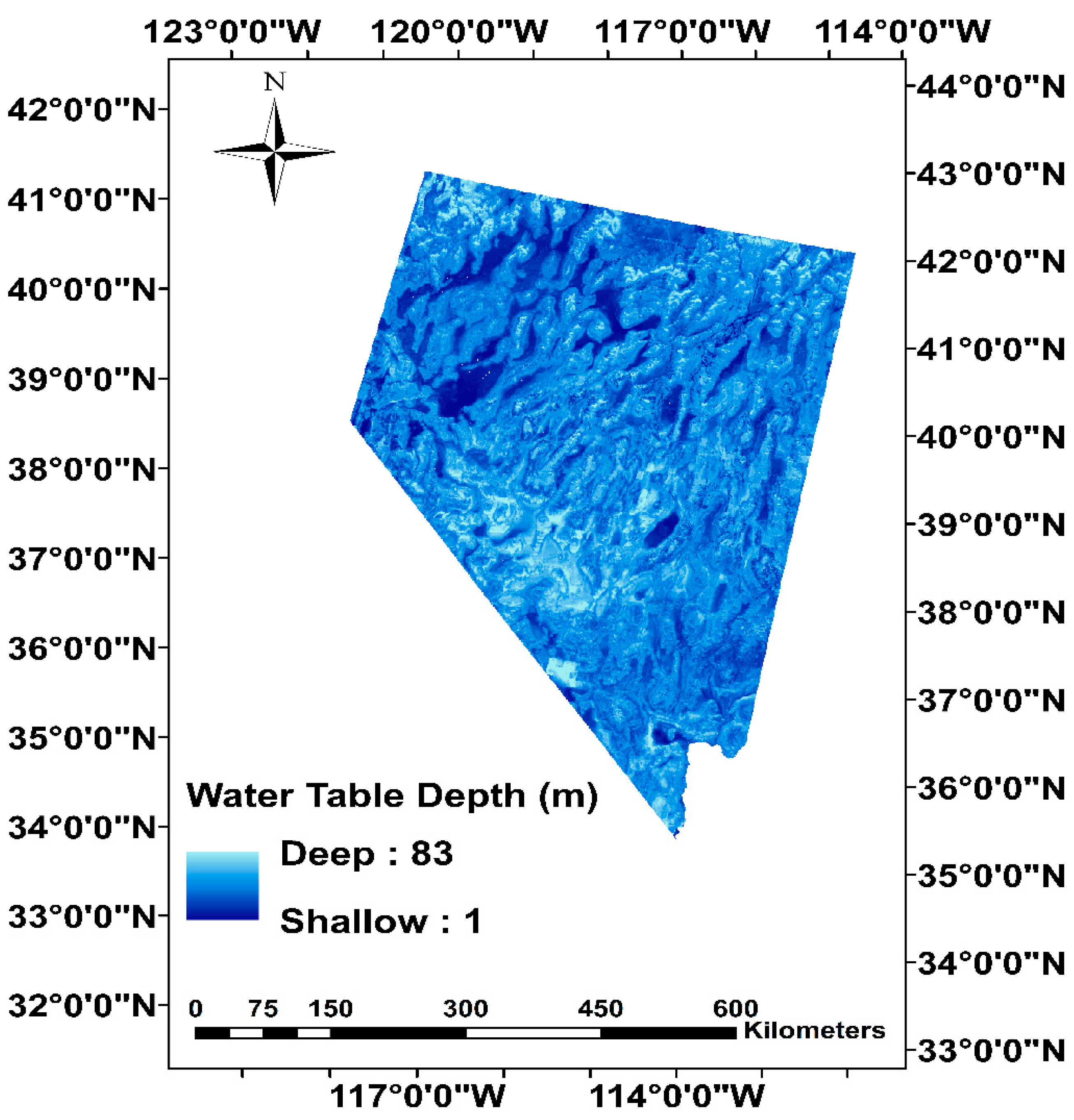
- Ecosystems dependent on the subsurface expression of groundwater: terrestrial vegetation that uses shallow groundwater (commonly referred to as phreatophytes). The water table can be considered shallow if it is less or equal to 10 m in depth [3], intermediate if it is between 10 m and 30 m, and deep if it is greater than 30 m. Plants can access groundwater by extending their roots to the water table and capillary fringe right above it. The roots of phreatophytes extend up to 3 m to almost 15 m below the land surface depending on the species [4].
- Aquifer and cave ecosystems: these include fractured rock, karstic, and alluvial aquifers, hyporheic zones of rivers and floodplains (saturated interstitial area beneath and alongside a stream bed where shallow groundwater and surface water mix), and stygofauna (organisms living in groundwater systems or aquifers).
1.1. Ecohydrology of GDEs
1.2. Research Objectives
2. Materials and Methods
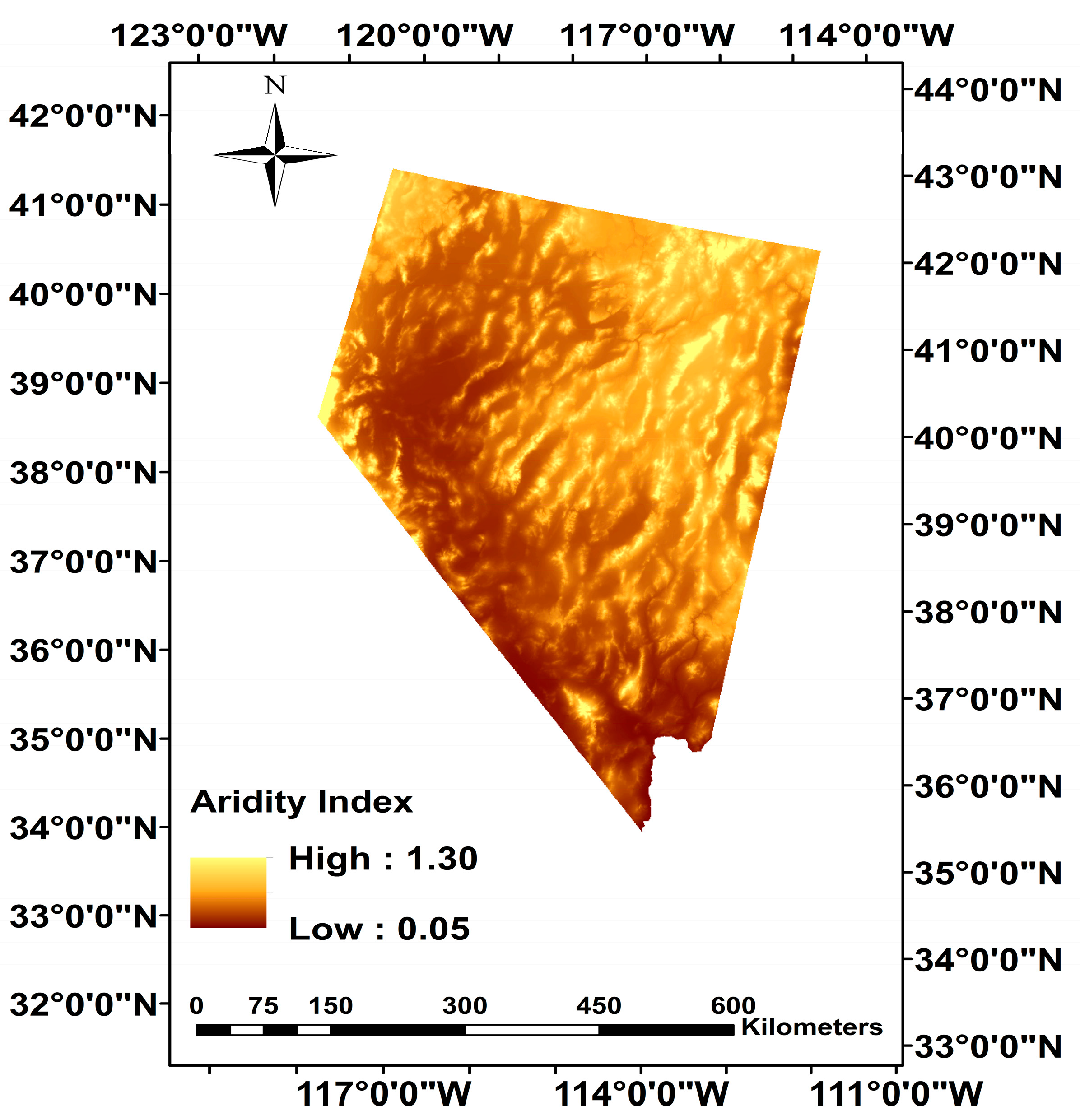
2.1. Study Area
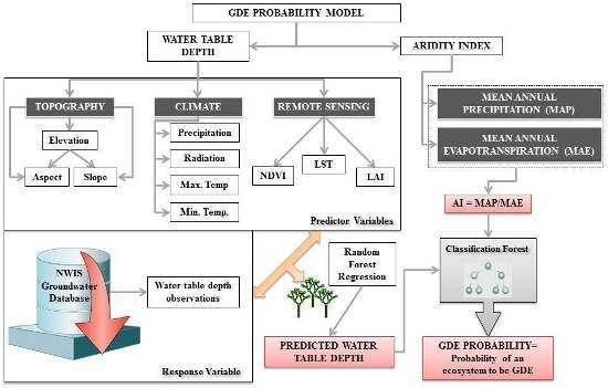
2.2. Predictor Variables
2.3. Response Variable
2.3.1. Groundwater Discharge as Evapotranspiration
2.3.2. Potential Areas of Groundwater Discharge
2.3.3. Phreatophytic Land-Cover Map of the Northern and Central Great Basin Ecoregion
2.4. Modeling
2.5. Evaluation of Model Performance
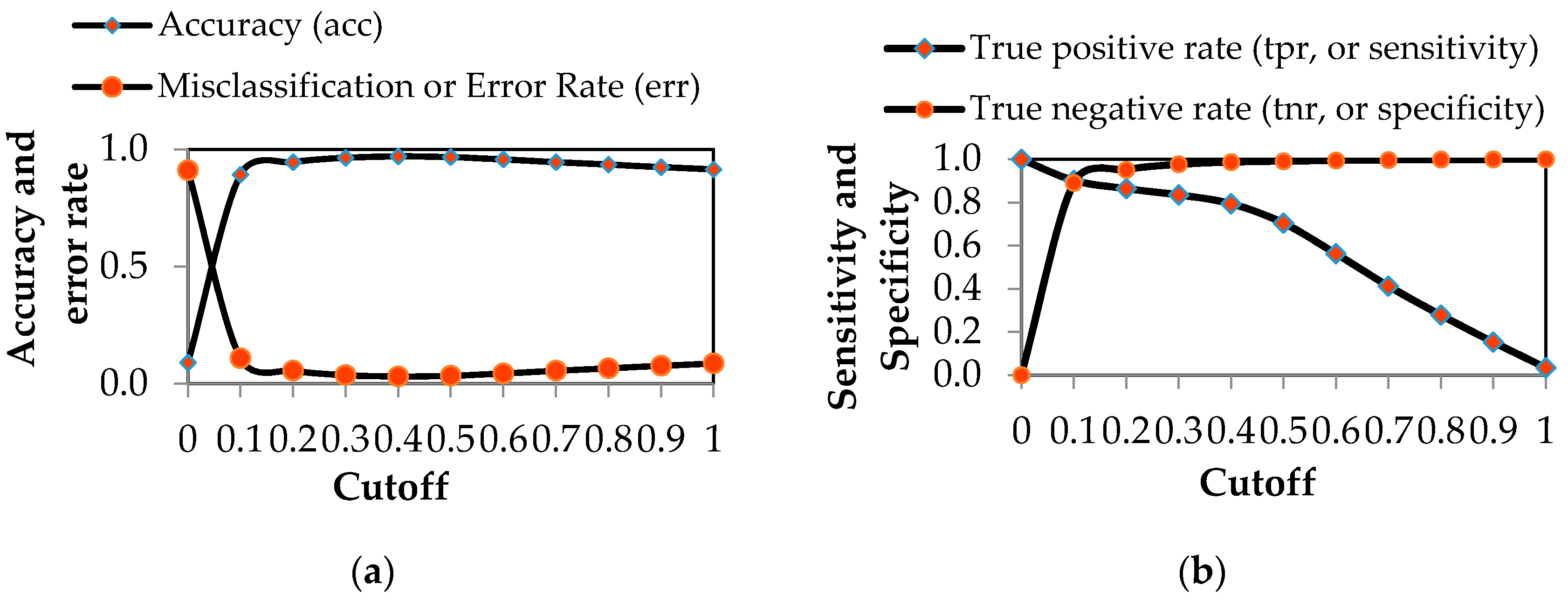
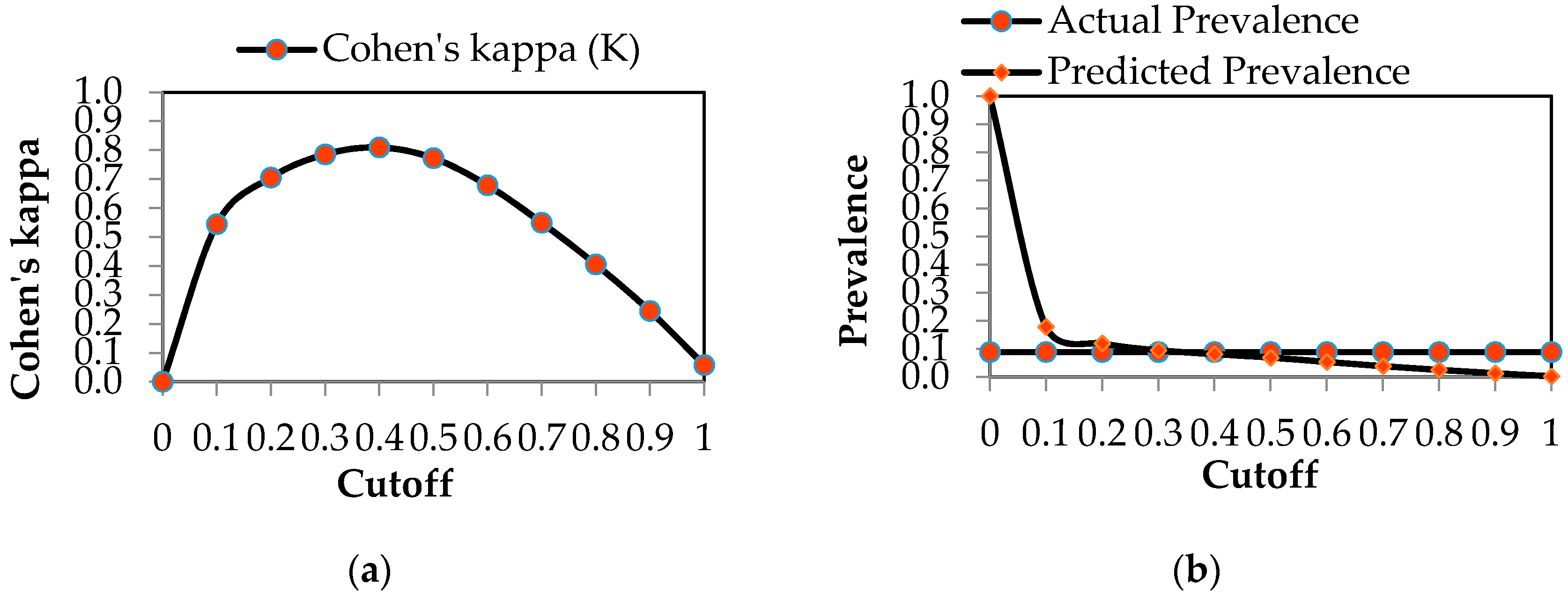
2.5.1. Threshold-Dependent Accuracy Measures
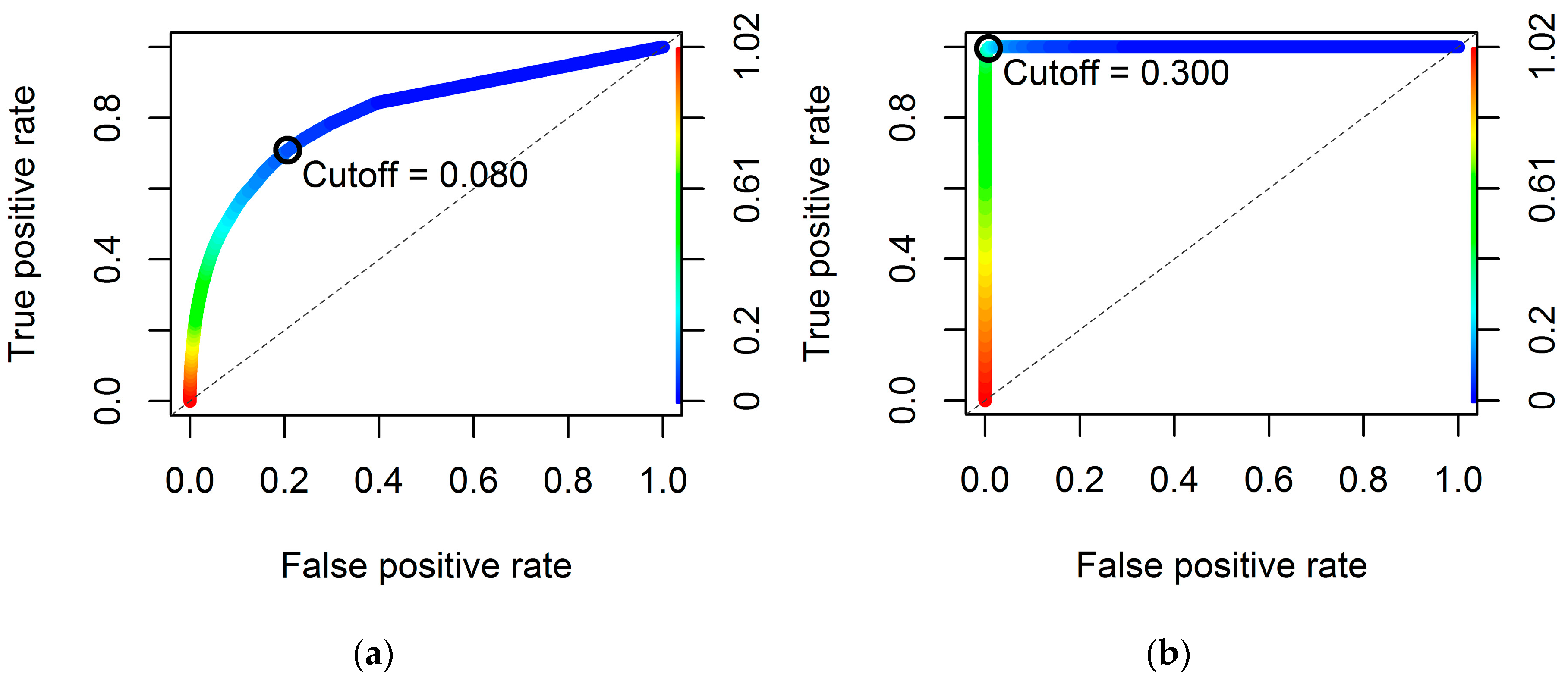
2.5.2. Model Selection Using ROC Curves
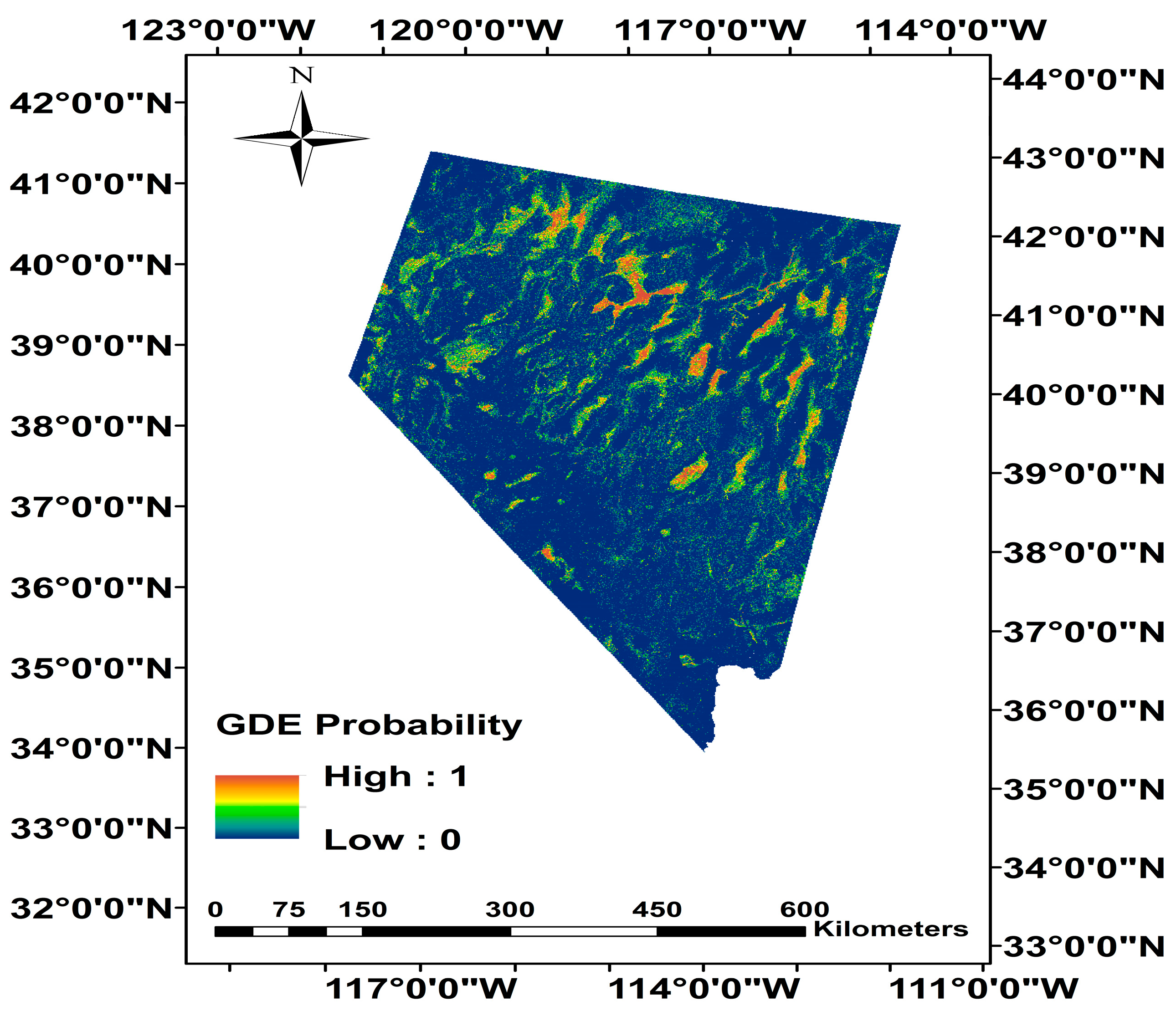
3. Results
Random Forest Performance Summary
4. Discussion
5. Conclusions
Acknowledgments
Author Contributions
Conflicts of Interest
References
- Glasser, S.; Gauthier-Warinner, J.; Keely, J.; Gurrieri, J.; Tucci, P.; Summers, P.; Wireman, M.; McCormack, K. Technical Guide to Managing Ground Water Resources; United States Department of Agriculture: Washington, DC, USA, 2007.
- Eamus, D. Identifying Groundwater Dependent Ecosystems: A Guide for Land and Water Managers; Australian Government, Land and Water Australia: Sydney, Australia, 2009.
- Contreras, S.; Jobbágy, E.G.; Villagra, P.E.; Nosetto, M.D.; Puigdefábregas, J. Remote sensing estimates of supplementary water consumption by arid ecosystems of central Argentina. J. Hydrol. 2011, 397, 10–22. [Google Scholar] [CrossRef]
- Mathie, A.M.; Welborn, T.L.; Susong, D.D.; Tumbusch, M.L. Phreatophytic Land-Cover Map of the Northern and Central Great Basin Ecoregion: California, Idaho, Nevada, Utah, Oregon, and Wyoming; U.S. Geological Survey: Reston, VA, USA, 2011.
- Lawford, R.; Strauch, A.; Toll, D.; Fekete, B.; Cripe, D. Earth observations for global water security. Curr. Opin. Environ. Sustain. 2013, 5, 633–643. [Google Scholar] [CrossRef]
- Münch, Z.; Conrad, J. Remote sensing and GIS based determination of groundwater dependent ecosystems in the Western Cape, South Africa. Hydrogeol. J. 2006, 15, 19–28. [Google Scholar] [CrossRef]
- Merz, S.K. Atlas of Groundwater Dependent Ecosystems (GDE Atlas); Australian Government, National Water Commission: Melbourne, Australia, 2012.
- Colvin, C.; Le Maitre, D.; Hughes, S. Assessing Terrestrial Groundwater Dependent Ecosystems in South Africa; Water Research Commission: Pretoria, South Africa, 2003. [Google Scholar]
- Gow, L.; Brodie, R.S.; Green, R.; Punthakey, J.; Woolley, D.; Redpath, P.; Bradburn, A. Identification and monitoring GDEs using MODIS time series: Hat Head National Park—A case study. In Groundwater 2010: The Challenge of Sustainable Management; National Convention Centre: Canberra, Australia, 2010. [Google Scholar]
- Werstak, C.E.; Housman, I.; Maus, P.; Fisk, H.; Gurrieri, J.; Carlson, C.P.; Johnston, B.C.; Stratton, B.; Hurja, J.C. Groundwater-Dependent Ecosystem Inventory Using Remote Sensing, RSAC-10011-RPT1; Remote Sensing Applications Center: Salt Lake City, UT, USA, 2012. [Google Scholar]
- Heidel, B.; Rodemaker, E. Inventory of Peatland Systems in the Beartooth Mountains, Shoshone National Forest; Environmental Protection Agency: Laramie, WY, USA, 2008.
- Brown, J.; Wyers, A.; Bach, L.; Aldous, A. Groundwater-Dependent Biodiversity and Associated Threats: A Statewide Screening Methodology and Spatial Assessment of Oregon; The Nature Conservancy: Arlington, VA, USA, 2009. [Google Scholar]
- Howard, J.; Merrifield, M. Mapping groundwater dependent ecosystems in California. PLoS ONE 2010, 5. [Google Scholar] [CrossRef] [PubMed]
- Brown, J.; Bach, L.; Aldous, A.; Wyers, A.; DeGagné, J. Groundwater-dependent ecosystems in Oregon: An assessment of their distribution and associated threats. Front. Ecol. Environ. 2011, 9, 97–102. [Google Scholar] [CrossRef]
- Elith, J.; Leathwick, J.R. Species Distribution Models: Ecological Explanation and Prediction across Space and Time. Annu. Rev. Ecol. Evol. Syst. 2009, 40, 677–697. [Google Scholar] [CrossRef]
- Manel, S.; Dias, J.M.; Buckton, S.T.; Ormerod, S.J. Alternative methods for predicting species distribution: An illustration with Himilayan river birds. J. Appl. Ecol. 1999, 36, 734–747. [Google Scholar] [CrossRef]
- Kath, J.; Le Brocque, A.; Leyer, I.; Mosner, E. Hydrological and land use determinants of Eucalyptus camaldulensis occurrence in floodplain wetlands. Austral Ecol. 2014, 39, 643–655. [Google Scholar] [CrossRef]
- Leyer, I. Predicting plant species’ responses to river regulation: The role of water level fluctuations. J. Appl. Ecol. 2005, 42, 239–250. [Google Scholar] [CrossRef]
- Kath, J.; Powell, S.; Reardon-Smith, K.; El Sawah, S.; Jakeman, A.J.; Croke, B.F.W.; Dyer, F.J. Groundwater salinization intensifies drought impacts in forests and reduces refuge capacity. J. Appl. Ecol. 2015, 52, 1116–1125. [Google Scholar] [CrossRef]
- Cunningham, S.C.; Thomson, J.R.; Mac Nally, R.; Read, J.; Baker, P.J. Groundwater change forecasts widespread forest dieback across an extensive floodplain system. Freshw. Biol. 2011, 56, 1494–1508. [Google Scholar] [CrossRef]
- Wilson, K.A.; Westphal, M.I.; Possingham, H.P.; Elith, J. Sensitivity of conservation planning to different approaches to using predicted species distribution data. Biol. Conserv. 2005, 122, 99–112. [Google Scholar] [CrossRef]
- Pérez Hoyos, I.; Krakauer, N.; Khanbilvardi, R.; Armstrong, R. A review of advances in the identification and characterization of groundwater dependent ecosystems using geospatial technologies. Geosciences 2016, 6. [Google Scholar] [CrossRef]
- Batelaan, O.; Witte, J.P.M. Ecohydrology and groundwater dependent terrestrial ecosystems. In Proceedings of the 28th Annual Conference of the International Association of Hydrogeologists (Irish Group), Tullamore, Ireland, 22–23 April 2008; pp. 1–8.
- Rodriguez-Iturbe, I. Ecohydrology: A hydrologic perspective of climate-soil-vegetation dynamics. Water Resour. Res. 2000, 36, 3–9. [Google Scholar] [CrossRef]
- Froend, R.; Loomes, R.; Horwitz, P.; Bertuch, M.; Storey, A.; Bamford, M. Study of Ecological Water Requirements on the Gnangara and Jandakot Mounds under Section 46 of the Environmental Protection Act Task 2: Determination of Ecological Water Requirements; Center for Ecosystem Management: Perth, Australia, 2004. [Google Scholar]
- Kløve, B.; Ala-aho, P.; Bertrand, G.; Boukalova, Z.; Ertürk, A.; Goldscheider, N.; Ilmonen, J.; Karakaya, N.; Kupfersberger, H.; Kvoerner, J.; et al. Groundwater dependent ecosystems. Part I: Hydroecological status and trends. Environ. Sci. Policy 2011, 14, 770–781. [Google Scholar] [CrossRef]
- Laio, F.; Tamea, S.; Ridolfi, L.; D’Odorico, P.; Rodriguez-Iturbe, I. Ecohydrology of groundwater-dependent ecosystems: 1. Stochastic water table dynamics. Water Resour. Res. 2009, 45. [Google Scholar] [CrossRef]
- Guswa, A.J.; Celia, M.; Rodriguez-Iturbe, I. Models of soil moisture dynamics in ecohydrology: A comparative study. Water Resour. Res. 2002, 38. [Google Scholar] [CrossRef]
- Guswa, A.J. Soil-moisture limits on plant uptake: An upscaled relationship for water-limited ecosystems. Adv. Water Resour. 2005, 28, 543–552. [Google Scholar] [CrossRef]
- Laio, F. A vertically extended stochastic model of soil moisture in the root zone. Water Resour. Res. 2006, 42, 1–10. [Google Scholar] [CrossRef]
- Laio, F.; Porporato, A.; Fernandez-Illescas, C.; Rodriguez-Iturbe, I. Plants in water-controlled ecosystems: Active role in hydrologic processes and response to water stress. Adv. Water Resour. 2001, 24, 745–762. [Google Scholar] [CrossRef]
- Porporato, A.; D’Odorico, P.; Laio, F.; Ridolfi, L.; Rodriguez-Iturbe, I. Ecohydrology of water-controlled ecosystems. Adv. Water Resour. 2002, 25, 1335–1348. [Google Scholar] [CrossRef]
- Rodríguez-Iturbe, I.; Porporato, A. Ecohydrology of Water-Controlled Ecosystems; Soil Moisture and Plant Dynamics; Cambridge University Press: Cambridge, UK, 2004. [Google Scholar]
- Rodriguez-Iturbe, I.; Porporato, A.; Ridolfi, L.; Isham, V.; Coxi, D.R. Probabilistic modelling of water balance at a point: The role of climate, soil and vegetation. Proc. R. Soc. Lond. A Math. Phys. Eng. Sci. 1999, 455, 3789–3805. [Google Scholar] [CrossRef]
- Tamea, S.; Laio, F.; Ridolfi, L.; D’Odorico, P.; Rodriguez-Iturbe, I. Ecohydrology of groundwater-dependent ecosystems: 2. Stochastic soil moisture dynamics. Water Resour. Res. 2009, 45. [Google Scholar] [CrossRef]
- D’odorico, P.; Laio, F.; Porporato, A.; Ridolfi, L.; Rinaldo, A.; Rodriguez, I. Ecohydrology of Terrestrial Ecosystems. Bioscience 2010, 60, 898–907. [Google Scholar] [CrossRef]
- Asbjornsen, H.; Goldsmith, G.R.; Alvarado-Barrientos, M.S.; Rebel, K.; Van Osch, F.P.; Rietkerk, M.; Chen, J.; Gotsch, S.; Tobón, C.; Geissert, D.R.; et al. Ecohydrological advances and applications in plant-water relations research: A review. J. Plant Ecol. 2011, 4, 3–22. [Google Scholar] [CrossRef]
- Sinclair Knight Merz Pty. Ltd. Environmental Water Requirements to Maintain Groundwater Dependent Ecosystems; Commonwealth of Australia: Canberra, Australia, 2001.
- Richardson, S.; Irvine, E.; Froend, R.; Boon, P.; Barber, S.; Bonneville, B. Australian Groundwater Dependent Ecosystems Toolbox Part 1: Assessment Framework; National Water Commission: Canberra, Australia, 2011.
- Dresel, P.E.; Clark, R.; Cheng, X.; Reid, M.; Terry, A.; Fawcett, J.; Cochrane, D. Mapping Terrestrial Groundwater Dependent Ecosystems: Method Development and Example Output; Department of Primary Industries: Melbourne, Australia, 2010.
- Freeman, E.A.; Moisen, G.G. A comparison of the performance of threshold criteria for binary classification in terms of predicted prevalence and kappa. Ecol. Model. 2008, 217, 48–58. [Google Scholar] [CrossRef]
- Perez Hoyos, I.C.; Krakauer, N.; Khanbilvardi, R. Random Forest for Identification and Characterization of Groundwater Dependent Ecosystems. WIT Trans. Ecol. Environ. 2015, 196, 89–100. [Google Scholar]
- Weisberg, P. Nevada Vegetation Overview. Available online: http://www.onlinenevada.org/articles/nevada-vegetation-overview (accessed on 14 November 2015).
- Pritchett, D.; Manning, S.J. Response of an Intermountain Groundwater-Dependent Ecosystem to Water Table Drawdown. West. N. Am. Nat. 2012, 72, 48–59. [Google Scholar] [CrossRef]
- Pritchett, D.W.; Manning, S.J. Effects of Fire and Groundwater Extraction on Alkali Meadow Habitat in Owens Valley, California. Madroño 2009, 56, 89–98. [Google Scholar] [CrossRef]
- Aldous, A.R.; Bach, L.B. Hydro-ecology of groundwater-dependent ecosystems: Applying basic science to groundwater management. Hydrol. Sci. J. 2014, 59, 530–544. [Google Scholar] [CrossRef]
- Roberts, J.J.; Best, B.D.; Dunn, D.C.; Treml, E.A.; Halpin, P.N. Environmental Modelling & Software Marine Geospatial Ecology Tools: An integrated framework for ecological geoprocessing with ArcGIS, Python, R, MATLAB, and C++. Environ. Model. Softw. 2010, 25, 1197–1207. [Google Scholar]
- Threneau, T.; Atkinson, B.; Ripley, B. Package “rpart”: Recursive Partitioning and Regression Trees; CRANR Project: Rochester, NY, USA, 2015; pp. 1–34. [Google Scholar]
- Liaw, A.; Wiener, M. Classification and Regression by Random Forest. R News 2002, 2, 18–22. [Google Scholar]
- R Foundation for Statistical Computing. R Development Core Team: A Language and Environment for Statistical Computing; R Core Team: Vienna, Austria, 2011. [Google Scholar]
- ESRI ArcGIS Desktop: Release 10.2. Environmental Systems Research Institute: Redlands, USA, 2013.
- Middleton, N.; Thomas, D. World Atlas of Desertification, 2nd ed.; United Nations Environment Program, Ed.; Routledge: London, UK, 1997. [Google Scholar]
- Fan, Y.; Li, H.; Miguez-Macho, G. Global Patterns of Groundwater Table Depth. Science 2013, 339, 940–943. [Google Scholar] [CrossRef] [PubMed]
- Perez Hoyos, I.C.; Krakauer, N.; Khanbilvardi, R. Prediction of water table depth from geospatial and remote sensing data using random forests. WIT Int. J. Sustain. Dev. Plan. 2016. submitted. [Google Scholar]
- Zomer, R.J.; Trabucco, A.; Bossio, D.A.; Verchot, L.V. Climate change mitigation: A spatial analysis of global land suitability for clean development mechanism afforestation and reforestation. Agric. Ecosyst. Environ. 2008, 126, 67–80. [Google Scholar] [CrossRef]
- Zomer, J.R.; Bossio, A.D.; Trabucco, A.; Yuanjie, L.; Gupta, C.D.; Singh, P.V. Trees and Water: Smallholder Agroforestry on Irrigated Lands in Northern India; International Water Management Institute: Colombo, Sri Lanka, 2007. [Google Scholar]
- Piper, M.E.; Loh, W.-Y.; Smith, S.S.; Japuntich, S.J.; Baker, T.B. Using decision tree analysis to identify risk factors for relapse to smoking. Subst. Use Misuse 2011, 46, 492–510. [Google Scholar] [CrossRef] [PubMed]
- Buto, S.G.; Sweetkind, D.S. 1:1,000,000-Scale Hydrographic Areas and Flow Systems for the Great Basin Carbonate and Alluvial Aquifer System of Nevada, Utah, and Parts of Adjacent States; U.S. Geological Survey: Reston, VA, USA, 2011.
- Batelaan, O.; De Smedt, F.; Triest, L. Regional groundwater discharge: Phreatophyte mapping, groundwater modelling and impact analysis of land-use change. J. Hydrol. 2003, 275, 86–108. [Google Scholar] [CrossRef]
- Tóth, J. Groundwater Discharge: A Common Generator of Diverse Geologic and Morphologic Phenomena. Int. Assoc. Sci. Hydrol. Bull. 1971, 16, 7–24. [Google Scholar] [CrossRef]
- Klijn, F.; Witte, J.P.M. Eco-hydrology: Groundwater flow and site factors in plant ecology. Hydrogeol. J. 1999, 7, 65–77. [Google Scholar] [CrossRef]
- Rosenberry, D.O.; Striegl, R.G.; Hudson, D.C. Plants as indicatosr of focused ground water discharge to a Northern Minnesota Lake. Ground Water 2000, 38, 296–303. [Google Scholar] [CrossRef]
- Laczniak, R.J.; Moreo, M.T.; Smith, J.L.; Harper, D.P.; Welborn, T.L. Potential Areas of Ground-Water Discharge in the Basin and Range Carbonate-Rock Aquifer System, White Pine County, Nevada, and Adjacent Parts of Nevada and Utah; U.S. Geological Survey: Reston, VA, USA, 2007.
- Provost, F.; Domingos, P. Well-Trained PETs: Improving Probability Estimation Trees; New York University: New York, NY, USA, 2000. [Google Scholar]
- Prasad, A.M.; Iverson, L.R.; Liaw, A. Newer Classification and Regression Tree Techniques: Bagging and Random Forests for Ecological Prediction. Ecosystems 2006, 9, 181–199. [Google Scholar] [CrossRef]
- Waljee, A.K.; Higgins, P.D.R.; Singal, A.G. A primer on predictive models. Clin. Transl. Gastroenterol. 2014, 5. [Google Scholar] [CrossRef] [PubMed]
- Moons, K.G.M.; Royston, P.; Vergouwe, Y.; Grobbee, D.E.; Altman, D.G. Prognosis and prognostic research: What, why, and how? BMJ 2009, 338. [Google Scholar] [CrossRef] [PubMed]
- Chawla, N.; Cieslak, D. Evaluating probability estimates from decision trees. Am. Assoc. Artif. Intell. 2006, 23, 18–23. [Google Scholar]
- Provost, F.; Domingos, P. Tree Induction for Probability-based Ranking. Mach. Learn. 2003, 52, 199–215. [Google Scholar] [CrossRef]
- Zadrozny, B.; Elkan, C. Learning and making decisions when costs and probabilities are both unknown. In Proceedings of the Seventh International Conference on Knowledge Discovery and Data Mining, San Diego, CA, USA, 21–24 August 2001; pp. 204–213.
- Moisen, G.G.; Freeman, E.A.; Blackard, J.A.; Frescino, T.S.; Zimmermann, N.E.; Edwards, T.C. Predicting tree species presence and basal area in Utah: A comparison of stochastic gradient boosting, generalized additive models, and tree-based methods. Ecol. Model. 2006, 199, 176–187. [Google Scholar] [CrossRef]
- Fawcett, T. An introduction to ROC analysis. Pattern Recognit. Lett. 2006, 27, 861–874. [Google Scholar] [CrossRef]
- Swets, J.A. Measuring the Accuracy of Diagnostic Systems. Science 1988, 240, 1285–1293. [Google Scholar] [CrossRef] [PubMed]
- Fielding, A.H.; Bell, J.F. A review of methods for the assessment of prediction errors in conservation presence/absence models. Environ. Conserv. 1997, 24, 38–49. [Google Scholar] [CrossRef]
- Manel, S.; Ceri Williams, H.; Ormerod, S.J. Evaluating presence-absence models in ecology: The need to account for prevalence. J. Appl. Ecol. 2001, 38, 921–931. [Google Scholar] [CrossRef]
- Krakauer, N.Y.; Grossberg, M.D.; Gladkova, I.; Aizenman, H. Information content of seasonal forecasts in a changing climate. Adv. Meteorol. 2013, 2013. [Google Scholar] [CrossRef]
- Allouche, O.; Tsoar, A.; Kadmon, R. Assessing the accuracy of species distribution models: Prevalence, kappa and the true skill statistic (TSS). J. Appl. Ecol. 2006, 43, 1223–1232. [Google Scholar] [CrossRef]
- Viera, A.J.; Garrett, J.M. Understanding interobserver agreement: The kappa statistic. Fam. Med. 2005, 37, 360–363. [Google Scholar] [PubMed]
- Eamus, D.; Zolfaghar, S.; Villalobos-Vega, R.; Cleverly, J.; Huete, A. Groundwater-dependent ecosystems: Recent insights from satellite and field-based studies. Hydrol. Earth Syst. Sci. 2015, 19, 4229–4256. [Google Scholar] [CrossRef]
- Lv, J.; Wang, X.S.; Zhou, Y.; Qian, K.; Wan, L.; Eamus, D.; Tao, Z. Groundwater-dependent distribution of vegetation in Hailiutu River catchment, a semi-arid region in China. Ecohydrology 2013, 6, 142–149. [Google Scholar] [CrossRef]
- Jin, X.M.; Schaepman, M.E.; Clevers, J.G.P.W.; Su, Z.B.; Hu, G.C. Groundwater Depth and Vegetation in the Ejina Area, China. Arid Land Res. Manag. 2011, 25, 194–199. [Google Scholar] [CrossRef]
- Foster, S.; Koundouri, P.; Tuinhof, A.; Kemper, K.; Nanni, M.; Garduño, H. Groundwater Dependent Ecosystems: The Challenge of Balanced Assessment and Adequate Conservation; The World Bank: Washington, DC, USA, 2006. [Google Scholar]


| Datasets | Mapping Scale or Spatial Resolution | Mapped Features | Spatial Extent | Data Source | Reference |
|---|---|---|---|---|---|
| Groundwater discharge as evapotranspiration | 1:1,000,000-scale map (Horizontal accuracy estimation of 550 m) | Outer extent of preatophyte areas | Great Basin carbonate and alluvial aquifer system. Includes portions of Nevada, Utah, California, and Idaho | Data compiled from previous studies: BARCAS, DVRFS, Eastern Nevada, and RASA. These studies are a combination of satellite, aerial imagery, field studies, and visual verification. | [58] |
| Potential areas of ground-water discharge | 1:1,000,000-scale map (Horizontal accuracy estimation of 550 m) | Outer extent of preatophyte areas | Eastern Nevada and Western Utah | USGS and SNWA data mapped during aerial field reconnaissance. Field verification was done using GPS and visual verification. | [63] |
| Phreatophytic Land-Cover Map of the Northern and Central Great Basin Ecoregion: California, Idaho, Nevada, Utah, Oregon, and Wyoming | 30 m | Phreatophytic vegetation | Northern and Central Great Basin Ecoregion: California, Idaho, Nevada, Utah, Oregon, and Wyoming | The data are based on the combination of land cover phreatophytic vegetation classes (obtained from Shrub Map and GAP data which are both a combiation of satellite imagery with digital elevation model derived datasets). | [4] |
| Accuracy Measure | Test Data (n = 85,888) | Training Data (n = 200,405) | ||
|---|---|---|---|---|
| CT | RF | CT | RF | |
| Area under the ROC curve (AUC) | 0.740 | 0.813 | 0.741 | 1.000 |
| Cutoff value | 0.224 | 0.080 | 0.224 | 0.300 |
| Accuracy (ACC) | 0.879 | 0.786 | 0.880 | 0.993 |
| True positive rate (Sensitivity) | 0.551 | 0.709 | 0.554 | 0.997 |
| True negative rate (Specificity) | 0.911 | 0.794 | 0.912 | 0.992 |
| Cohen’s kappa (K) | 0.384 | 0.277 | 0.386 | 0.957 |
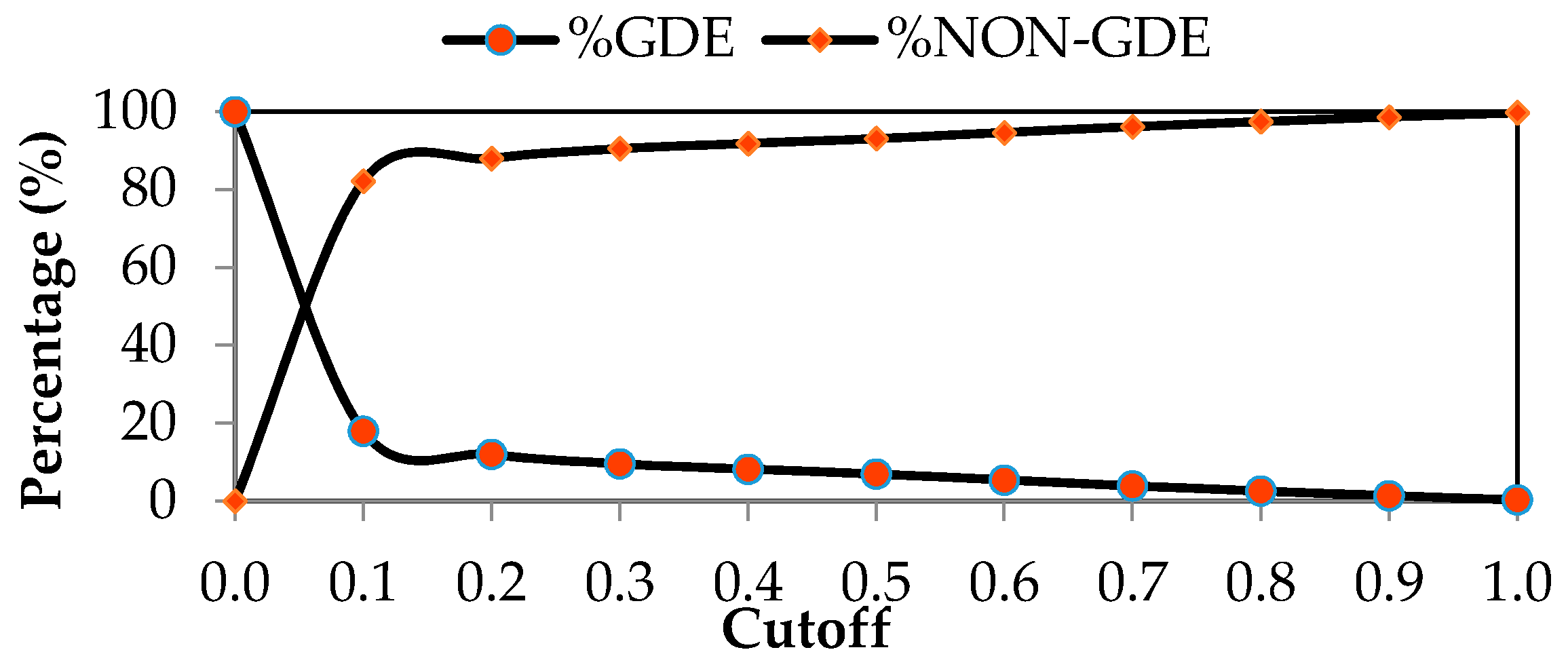
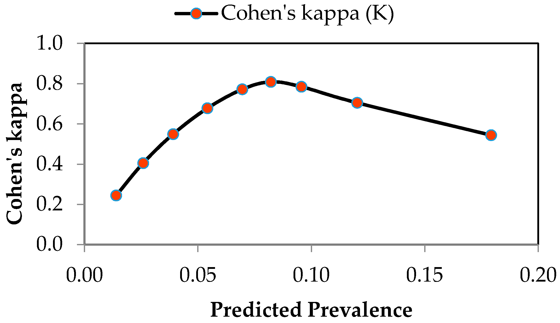
| Specified Cutoff | 0.0 | 0.1 | 0.2 | 0.3 | 0.4 |
|---|---|---|---|---|---|
| Number of pixels classified as GDEs | 286,291 | 51,294 | 34,407 | 27,359 | 23,500 |
| %GDE | 100.0 | 17.9 | 12.0 | 9.6 | 8.2 |
| Number of pixels classified as NON-GDEs | 0.000 | 234,997 | 251,884 | 258,932 | 262,791 |
| %NON-GDE | 0.0 | 82.1 | 88.0 | 90.4 | 91.8 |
| Accuracy (acc) | 0.089 | 0.892 | 0.945 | 0.964 | 0.970 |
| Misclassification or Error Rate (err) | 0.911 | 0.108 | 0.055 | 0.036 | 0.030 |
| True positive rate (tpr, or sensitivity) | 1.000 | 0.902 | 0.864 | 0.835 | 0.794 |
| True negative rate (tnr, or specificity) | 0.000 | 0.891 | 0.952 | 0.977 | 0.987 |
| Cohen’s kappa (K) | 0.000 | 0.544 | 0.705 | 0.785 | 0.809 |
| Specified Cutoff | 0.5 | 0.6 | 0.7 | 0.8 | 0.9 | 1.0 |
|---|---|---|---|---|---|---|
| Number of pixels classified as GDEs | 19,900 | 15,498 | 11,167 | 7387 | 3986 | 848 |
| %GDE | 7.0 | 5.4 | 3.9 | 2.6 | 1.4 | 0.3 |
| Number of pixels classified as NON-GDEs | 266,391 | 270,793 | 275,124 | 278,904 | 282,305 | 285,443 |
| %NON-GDE | 93.0 | 94.6 | 96.1 | 97.4 | 98.6 | 99.7 |
| Accuracy (acc) | 0.967 | 0.957 | 0.945 | 0.935 | 0.924 | 0.914 |
| Misclassification or Error Rate (err) | 0.033 | 0.043 | 0.055 | 0.065 | 0.076 | 0.086 |
| True positive rate (tpr, or sensitivity) | 0.704 | 0.562 | 0.412 | 0.277 | 0.152 | 0.033 |
| True negative rate (tnr, or specificity) | 0.992 | 0.995 | 0.997 | 0.999 | 1.000 | 1.000 |
| Cohen’s kappa (K) | 0.772 | 0.678 | 0.549 | 0.405 | 0.244 | 0.058 |
| Surface Water Shortage | Priority Stakeholder | Threshold Selection Criteria |
|---|---|---|
| No shortage | Environment—Local water resource, land planning, and environmental protection agencies | Required sensitivity |
| Moderate shortage | Humans and Environment (Rural, urban, industrial, tourism sectors, and Environment) | Predicted prevalence = Actual prevalence |
| High shortage | Humans (Rural, urban, industrial, tourism sectors) | Required specificity |
© 2016 by the authors; licensee MDPI, Basel, Switzerland. This article is an open access article distributed under the terms and conditions of the Creative Commons by Attribution (CC-BY) license (http://creativecommons.org/licenses/by/4.0/).
Share and Cite
Pérez Hoyos, I.C.; Krakauer, N.Y.; Khanbilvardi, R. Estimating the Probability of Vegetation to Be Groundwater Dependent Based on the Evaluation of Tree Models. Environments 2016, 3, 9. https://doi.org/10.3390/environments3020009
Pérez Hoyos IC, Krakauer NY, Khanbilvardi R. Estimating the Probability of Vegetation to Be Groundwater Dependent Based on the Evaluation of Tree Models. Environments. 2016; 3(2):9. https://doi.org/10.3390/environments3020009
Chicago/Turabian StylePérez Hoyos, Isabel C., Nir Y. Krakauer, and Reza Khanbilvardi. 2016. "Estimating the Probability of Vegetation to Be Groundwater Dependent Based on the Evaluation of Tree Models" Environments 3, no. 2: 9. https://doi.org/10.3390/environments3020009