Article

Understanding the Impact of Intensive Horticulture Land-Use Practices on Surface Water Quality in Central Kenya

Department of Earth and Environmental Studies, Montclair State University, Montclair, NJ 07043, USA
*
Author to whom correspondence should be addressed.
Environments 2015, 2(4), 521-545; https://doi.org/10.3390/environments2040521
Submission received: 9 July 2015 / Revised: 8 October 2015 / Accepted: 27 October 2015 / Published: 6 November 2015

Abstract

:
Rapid expansion of commercial horticulture production and related activities contribute to declining surface water quality. The study sought to understand the impacts on select rivers in Laikipia and Meru, production hotspots. The specific aims were (1) to identify prevailing surface water quality by examining variations of 14 physico-chemical parameters, and (2) to categorize measured surface water quality parameters into land use types highlighting potential pollutant source processes. Water samples were collected in July and August 2013 along 14 rivers in the study area. The data were analyzed using principal component analysis (PCA) and discriminant analysis (DA). Principal components (PCs) explained 70% of the observed total variability of water quality, indicating a prevalence of heavy metal traces (cadmium, phosphate, and zinc). These were linked to the rigorous use of phosphate fertilizers and copper-based agrochemicals in intensive farming. DA provided four significant (p < 0.05) discriminant functions, with 89.5% correct assignment enabling the association of land use with observed water quality. Concentrations of dissolved solids, electro-conductivity, and salinity spiked at locations with intensive small-scale and large-scale horticulture. Understanding the impacts of intensive commercial horticulture and land use practices on water quality is critical to formulating ecologically sound watershed management and pollution abatement plans.

1. Introduction

Surface streams and rivers are important sources of fresh water for domestic, industrial, and irrigation purposes in Kenya. The rapid rise of commercial horticulture [1,2,3,4,5] has impaired water quality, affecting the physico-chemical properties of surface waters [6,7,8]. Horticultural pollutants transported in runoff or through leaching into surface streams contribute to declining water quality that limits stream integrity and usefulness. The management of horticultural pollutants in watersheds with diverse land uses [9,10,11] is a complex process, and is often faced with the difficulty of separating effluents from different land processes and land use types. In addition, horticultural effluents are high in nitrogen and phosphorus, pesticide residues, and soil enhancements [7], which degrade water quality, making it unhealthy for human use, while also exposing the aquatic communities to habitation stress.
Since the late 1990s, Kenya’s demand for pesticides has been increasing, a trend attributable to horticulture farming [12]. Close to 7000 metric tons of pesticides are imported annually to meet the growing demand. Recently, [13] found high levels of pollutants and heavy metals (lead, mercury, and copper) in the Nairobi River and its tributaries. They highlighted a need to review the existing land use policy in the country in order to limit encroachment of unplanned land use activities into important watershed areas. Horticultural vegetable farmers use a wide variety of pesticides, including herbicides (e.g., linurex 50 wp, diurex 80 wp), insecticides (e.g., diazol 60 EC, methomex 90S), and fungicides (e.g., Folicur EW and dithane M45) [8]. Their work [8] is among the limited few recent studies documenting the prevalent use and mismanagement of pesticides in horticulture farming. Consequently, the extent of pollution and the dominance of organic and inorganic elements in surface streams and rivers draining horticultural watersheds surrounding the Mount Kenya region are poorly understood. Previous work on Lake Naivasha, which is surrounded by intensive horticulture, suggests that the practice has detrimental effects on the lake’s fresh water quality and quantity [7]. In the foot zones of Mount Kenya, where horticulture is rapidly expanding, Liniger et al. [14] identified a decline in surface flow and an increase in water abstraction by the farmers. Nevertheless, the study did not report water quality conditions despite a desire to create a long-term, sustainable water monitoring institution within the basin. Agrochemicals and fertilizers applied on agricultural lands are recognized as a main source of pollution to water systems, and are therefore a threat to the environment and human health [15]. Regular use of pesticides to ensure “pure” undefiled fresh produce free of insect marks promotes increased applications of agrochemicals, which may vary in degree of persistence in the environment. Long-term continued exposure to aquatic creatures, even when the environmental concentrations are not acutely toxic, is not sustainable and can become critical [16].
As often in practice, however, the intensification of agriculture is often accompanied by the use of additional agrochemicals, a common approach to maximize production per unit of land area [17]. Water contamination by heavy metals due to intensified agriculture, rapid urbanization, and industrialization is of global concern [18]. Commonly used basal and top-dressing fertilizers in intensive horticulture have a phosphorite base, which is high in heavy metals that are of environmental concern such as cadmium, uranium, and arsenic [19]. The long-term application of phosphorus (P) fertilizers contributes to cadmium build-up in soils [20] and global surveys of metals in P fertilizers corroborate the finding [15]. Also, other metals such as zinc and lead have shown positive correlations with increasing P concentrations in soils. Once in the soil, metals may accumulate, or even enter the food chain, through hyper-accumulating plants. They may also enter the surface streams through leaching and erosion processes. The use of contaminated surface waters for irrigation purposes propagates the pollution effect onto land as well [21]. Depending on regional application of agrochemicals, and more so the P fertilizers, the inputs of trace metals and metalloids into the agricultural soils and surface water may differ spatially.
In this work, sub-watersheds with intensive small-scale (SSHORT) and large-scale commercial horticulture (LSHORT) are considered in an effort to examine underlying characteristics in water quality. Clustering of intensive farming in specific sub-watersheds [22] accompanied by growing changes in land use and land cover pattern pose pollution risks to surface waters. In many cases, the water obtained from these streams is not screened for contaminants before use, which poses a public health concern. In this study, we intend to: (1) evaluate prevailing surface water quality by examining physico-chemical parameter variations in samples, and (2) categorize measured surface water quality parameters into land use types highlighting potential pollutant source processes.
Water quality monitoring studies commonly assess water quality indicators such as phosphate, nitrate, potassium, zinc, copper, cadmium, iron, sulfide, dissolved oxygen, pH, salinity, electrical conductivity, total dissolved substances, and water temperature. These indicators are critical for sustaining aquatic life, plants, humans, and animals [23,24,25,26]. Some of these parameters occur as rare earth elements and thus their occurrence in surface waters has been applied as tracers of anthropogenic processes in environmental studies [27].
To design better water resource management strategies, there is an urgent need for comprehensive water quality monitoring across the diverse land use platform in Kenya. Information on elemental composition in surface waters will help facilitate efficient policy decisions. However, diverse land use systems within sub-watersheds present a complex situation when tracking source processes, necessitating an application of combined methods of analyzing field data.
In this study, we adopt the commonly used principal component analysis (PCA) and discriminant analysis (DA) techniques to analyze water quality data. These techniques not only facilitate the analysis and interpretation of intricate water quality data [25,28,29], but also allow for an in-depth understanding of the prevailing surface water quality and the detection of source processes influencing water systems.
Following this introduction section, we will discuss the study area and methodology in detail. Results from the data analysis will be presented in the third section. The fourth section presents a discussion of these results, and we conclude the research with a summary and proposals for future research.

2. Materials and Methods

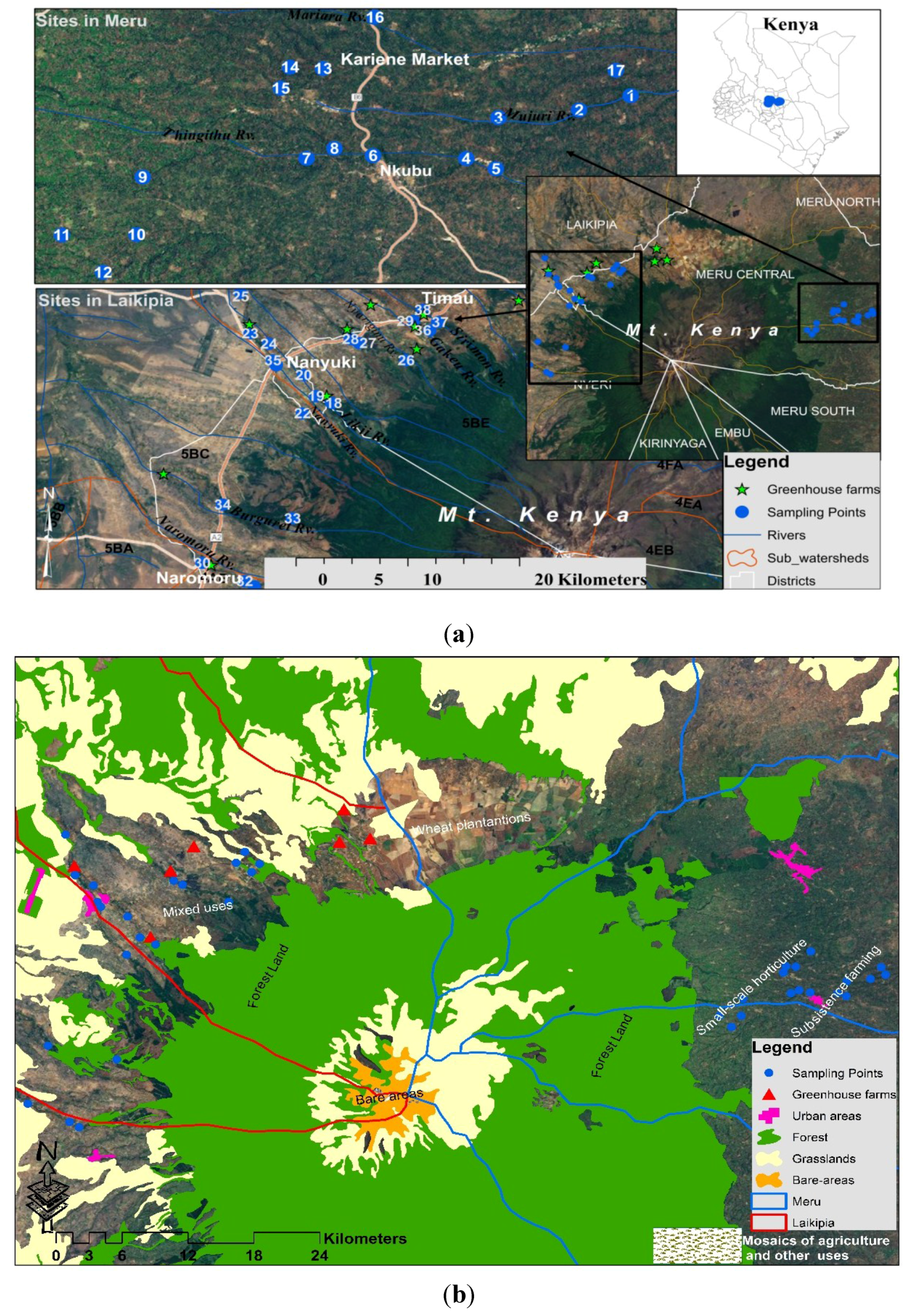
2.1. Study Area: Rivers in the Sub-Watersheds

This research focuses on the major rivers in the Laikipia and Meru central regions, which are major horticultural producing zones in Central Kenya. In Laikipia, export-oriented horticultural farming is mainly carried out by large-scale farms and a few small-scale farmers. Intensive horticulture farming in Meru is carried out by small-scale farmers on a contractual basis. The two regions are geographically separated by Mount Kenya Forest (Figure 1), an important source of fresh water. Major rivers in Laikipia include Likii, Nanyuki, Naromoru, and Burguret, which form tributaries to the Ewaso Nyiro River. In Meru, the major rivers are Kathita and Mutonga, which provide water for irrigation as well as human use. Because of the strong shadow effect of Mount Kenya, the adjoining Laikipia plateau is actually a semi-arid region, with a bimodal rainfall of ~450–750 mm/year [30]. Due to the low average annual rainfall, the dominant vegetation is Acacia and Themeda grass, which is typical of savanna environments [31]. Meru is on the northeast slopes of Mount Kenya, where the vegetation changes dramatically to thick mixed forest due to more annual rainfall varying between 1200 and 1500 mm [32]. The mean annual temperature is ~20 °C. Soils in the Laikipia area have formed as a result of volcanic activity along the Rift Valley. They are predominantly fertile, deep (>160 cm), rich in clay, well drained, and support diverse agricultural activities [33,34]. The soils in Meru are of two origins: (a) soils developed on volcanic material and (b) soils developed on basement system rocks. Volcanic-developed soils are mainly well drained, very deep, and contain red and friable clays (nitisols, andisols, and acrisols). Soils developed on basement system rocks are excessively drained, shallow to deep, red, with friable to firmly loamy sand to clay (luvisols, cambisols, lithosols) [35].
Surface waters in the area form a radial drainage pattern, characteristic of volcanic mountains of a relatively young drainage network [30]. In the upper zones of Mount Kenya, the rivers are fed by glacial and snow melt. As the river flow through the thick forest cover, they form dense networks of deeply incised tributaries, which find ways into the foot zones of the mountain, resulting in meandering and ephemeral tributaries. The headwaters are generally cold, but the temperature increases as they exit the forest. The transitional zones are experiencing increased anthropogenic perturbations (Figure 1a,b) in the form of land clearing on forest edges mainly for farming practices and settlements. The mid-waters in Laikipia flow through dense horticultural production zones characterized by greenhouses and open crop fields as well as urban areas with increased human settlements. The prevailing mix of land uses is a concern to the mid-water’s quality mainly due to nutrient-loaded horticultural effluents and municipal waste discharges. The lower reaches of the rivers in Laikipia have low river flow due to the overuse of the head- and mid-waters. Towards Meru, the rivers flow to Tana and Ura, and later to the Indian Ocean. Like Laikipia, forest-clearing to create farming land is common along the forest edges. These practices affect the quality and flow of surface waters in the study area.
Generally, five main land use practices exist in the study area: irrigation-dependent, all-season, large-scale intensive horticulture (LSHORT) (in greenhouses and also open fields); all-season, small-scale intensive horticulture (SSHORT), consisting of mainly vegetables for export, with farmers sub-contracted by large exporting companies; mixed agriculture (MAG) farming of subsistence and cash crops that depends on the prevailing rainfall; urban uses (including residential settlement, small industries/auto businesses, car washes, automobile repair shops); and forest. The mix of land uses and diverse waste effluents present a complex environmental management challenge to water resource managers.
Figure 1. Study area maps. (a) Shows sub-watersheds around Mount Kenya, the surface water sampling points, and towns. To the West is Laikipia, which represents a growing cluster of large-scale commercial horticulture; and to the East is Meru, consisting of a mix of subsistence farming and intensive small-scale contracted horticulture farmers. (b) Shows various land cover and land uses within the study area (data source—World Resources Institute (WRI) [36].
Environments 02 00521 g001

2.1.1. Field Sampling—Sites

Thirty-eight sampling sites were established across five land use types common in the region. Twenty-one sites were in Laikipia sub-watersheds, and 17 sites in Meru central sub-watersheds. The site selection was based on prior knowledge of the area and land use types, accessibility of rivers to conduct sampling, and also proximity to greenhouse farming (particularly in Laikipia where greenhouses are utilized). The sites in Laikipia were located on six main rivers, i.e., Nanyuki, Likii, Burgureti, Naromoru, Nyariginu, Sirimon, and Gakeu (See Table 1). Sampling sites in Meru were located on eight rivers, i.e., Mujuri, Thinghithu, Mariara, Njoe, Kithinu, Gitauga, Gatauga, and Kiuna Ndegwa. At each site, a grab sample was collected by directly filling a one-gallon sample bottle at various vertical depths at the center of the channel where water was well mixed. In deeper waters, sampling was done by lowering a weighted bottled on a rope or steel rod into the stream. Samples were representative of the site conditions under the different land use to enable accurate assessment of the study area with a minimum number of samples.
Table 1. Sampled sites (Site ID) and the respective rivers.
Site IDNameSite IDName
Site 1Mujuri Rv. (downstream)Site 20Likii Rv. near Likii high sch.(midstream)
Site 2Mujuri Rv. (midstream)Site 21Nanyuki Rv. below Bucaneer club (midstream)
Site 3Mujuri Rv. (upstream)Site 22Nanyuki Rv. at Mt.Kenya Safariclub (upstream)
Site 4Thingithu Rv. (downstream; quary)Site 23Nanyuki Rv. (downstream)
Site 5Thingithu Rv. Mujwa bridge (downstream)Site 24Likii Rv. near Likii (downstream)
Site 6Thingithu Rv. at Nkubu bridge (midstream)Site 25Likii Rv. and Nanyuki Rv. (downstream)
Site 7Kiuna Ndegwa Rv. (downstream)Site 26Nyariginu Rv. (upstream)
Site 8Thingithu Rv.(upstream)Site 27Nyariginu Rv. (midstream)
Site 9Kiuna Ndegwa Rv. (upstream)Site 28Nyariginu Rv. (midstream)
Site 10Kithinu Rv. (downstream)Site 29Gakeu stream (downstream)
Site 11Kithinu Rv. (upstream)Site 30Narumoru Rv. (downstream)
Site 12Kirimbia Rv. (midstream)Site 31Narumoru Rv. (upstream)
Site 13Gitauga Rv. (midstream)Site 32Narumoru Rv. (midstream)
Site 14Gakuri Rv. (midstream)Site 33Burguret Rv. (downstream)
Site 15Gatauga Rv. (midstream)Site 34Burguret Rv. (upstream)
Site 16Mariara below bridge (midstream)Site 35Nanyuki Rv. (midstream)
Site 17Njoe Rv. (downstream)Site 36Gakeu stream (upstream)
Site 18Likii Rv. (upstream)Site 37Sirimon Rv. (upstream)
Site 19Likii Rv. (midstream)Site 38Sirimon Rv. (downstream)

2.1.2. Field Measurement and Analysis

Water samples were collected during the months of July and August 2013. Data for 14 commonly used physico-chemical water quality indicators [23,26,37,38], i.e., phosphate, nitrate, potassium, zinc, copper, cadmium, iron, sulphide, dissolved oxygen, pH, salinity, electric-conductivity, total dissolved substances, and water temperature, were collected.
No rainfall events occurred during the sampling period and all samples were obtained between 9 a.m. and 11 a.m. to avoid the influence of increased temperatures over the parameters. GPS locations of all sites were recorded and field notes were taken, documenting the surrounding river/stream habitat characteristics, bank conditions, and other general observations that could be useful in result interpretation.
Measurements of water pH, water temperature (°C), salinity (mg/L), TDS (mg/L), and electrical conductivity (EC-µS/cm) were determined in situ by dipping an EXTECH EC500 meter into a subsample. For dissolved oxygen evaluation, sub-samples from the main grab sample were obtained and treated on site, and then later analyzed alongside other parameters. Since dissolved oxygen results are affected easily by factors including the contact with atmosphere, field quality assurance procedures require the DO sample to be “treated/fixed” by adding two drops of manganese sulfate solution (4167) and two drops of alkaline potassium iodide azide (7166). The sample is then inverted to mix and precipitate. Following this step, eight drops of sulfuric acid, 1:1 (6141 WT), are added, and the sample is mixed gently until the precipitate dissolves. When DO samples are treated in this manner, they allow enough time to return to the testing station for performance of the actual test procedures [39].
Field analytical procedures outlined for the SMART3 colorimeter, an EPA-accepted multisensory field instrument, were followed (the specific methods and codes are cited in parentheses): copper (bicinchoninic acid—CODE 3640); sulphide (methylene blue—CODE 3654-020); dissolved oxygen (Winkler colorimetric—CODE 3688); cadmium (Pan—CODE 4017-01); nitrate (zinc reduction—CODE 3689); zinc (Zincon—CODE 3667); iron (bipyridyl—CODE 3648); phosphate (ascorbic acid reduction—CODE 3653); and potassium (tetraphenylboron—CODE 3639) (Geotech Smart3 Colorimenter Manual, 2011). Samples collected were assumed representative of the water quality, not contaminated or altered from improper handling, to ensure strict standards of sampling procedures and guidelines set by the EPA.

2.1.3. Statistical Analysis of Water Quality Data

Principal Component Analysis (PCA)

PCA detects similarities and differences in water quality while pinpointing fewer important parameters that explain a high variability in samples. The technique is therefore useful in describing water quality with multiple variables. The generated principal components (PC) are uncorrelated new variables, obtained by multiplying the original correlated variables with the eigenvector loadings. The principal component (PCs) can be expressed as:
zij = ai1x1j + ai2x2j + ai3x3j +…+ aimxmj
where z is the component score, a is the component loading, x is the measured value of the variable, i is the component number, j is the sample number, and m is the total number of variables.
As a common practice, PCs with eigenvalues greater than one were retained since they explained the highest total variability in water quality. Biplots of the resulting scores and loading were also constructed. Biplots are considered a standard tool to present multivariate data, providing a meaningful investigation of the data structure. The arrangement and display of rays (loadings) is based on the overall correlation matrix [40]. Our use of biplots was mainly to enhance a profound understanding of system processes, while visualizing the pattern of spread and concentration of elements in water [41]. Compared to bivariate scatterplots, biplots provide an overall planar view of the multivariate relationships of the parameters [42].

2.1.4. Discriminant Analysis (DA)

Though PCA is able to reduce data dimensionality and complexity while providing parameters of great variability and similarity in waters in a study area, it lacks the statistical means of associating observed source variation (pollution) to particular processes or activities (land use) in the sub-watersheds. Discriminant analysis (DA), on the other hand, is commonly used in pattern recognition and interpretation [43,44]. The analytical approach classifies cases into categorically dependent values, where prior knowledge of the membership of objects to a particular group is essential [43]. Multiple quantitative attributes (in this study, water quality parameters) are used to discriminate between two or more occurring groups, providing a statistical classification of samples. In our study, DA was used to classify samples (sites) into five classes representing the main land use groups in the study area. DA was carried out using SPSS by defining water quality parameters as independent variables, and the land use types were considered dependent variables. Water quality indicators common to a land use type, e.g., nitrates and phosphorus are highly linked to agricultural land use, are grouped together and considered pollutants and processes of interest borne by that group [24]. DA also provides a classification accuracy assessment matrix where 100% accuracy indicates a perfect discrimination of sites based on water quality characteristics.

3. Results

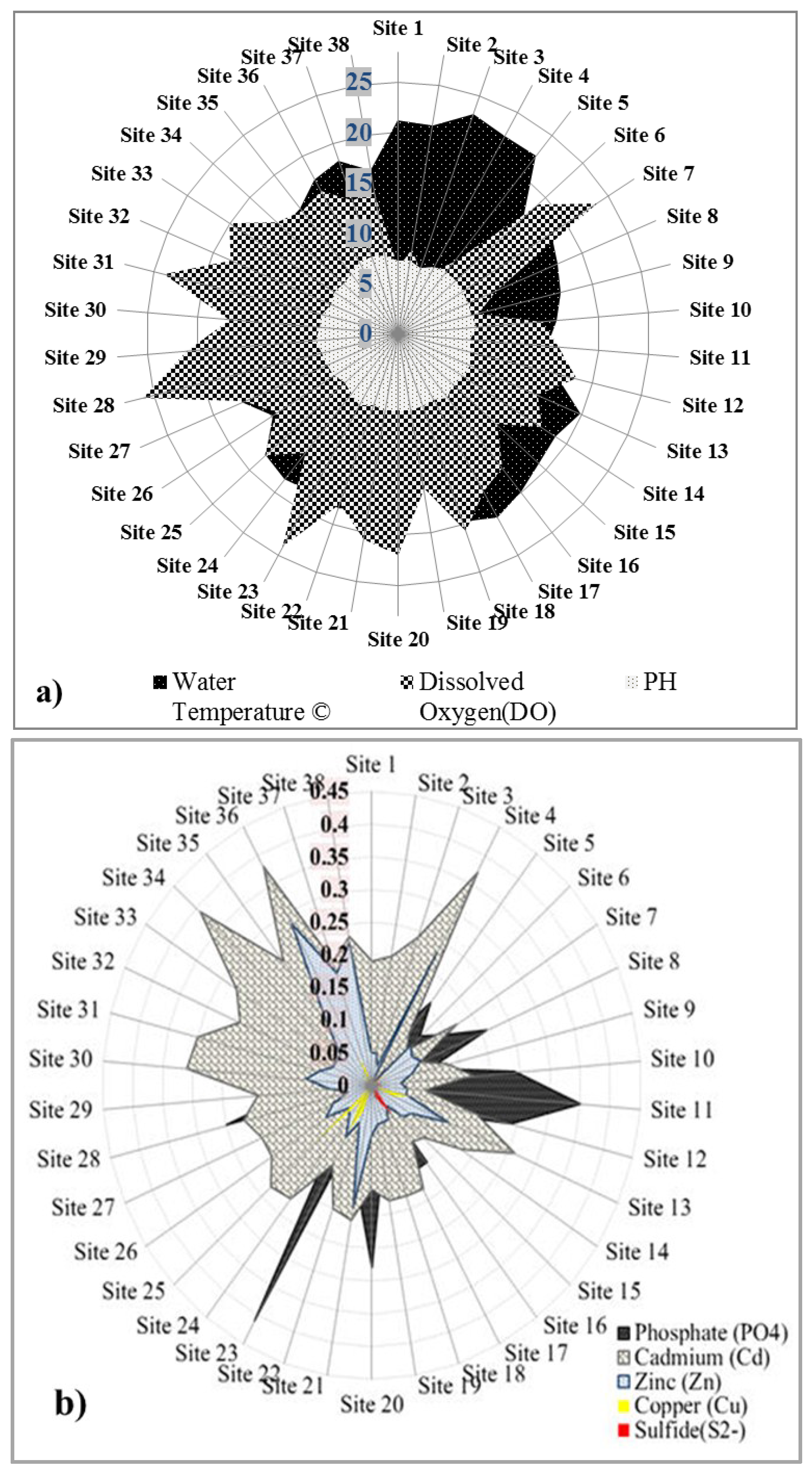
3.1. Field Data Description

Figure 2, Figure 3 and Figure 4 show variation of the physico-chemical water quality parameters, i.e., phosphate, nitrate, potassium, zinc, copper, cadmium, iron, dissolved oxygen, pH, salinity, EC, TDS, and water temperature (°C).
Results in Figure 2 show a positive direct relationship between the concentrations of EC, TDS, and salinity such that high (low) traces of TDS were accompanied by high (low) EC and salinity. The pattern is repeated for all stations except at site 3 (Figure 2). The concentration of the three elements is extraordinarily high at sites 13, 14, 15, 29, and 36 compared to other sites. Site 14 and site 15 are located on the Gakuri and Gatauga rivers, and both are tributaries to the Gitauga River where site 13 was located. The area surrounding these sites showed ongoing intensive SSHORT farming and very little stream bank cover. Likewise, sites 36 and 29 are located on the same river (Gakeu), with site 29 at the downstream of a large-scale horticulture farm. These results (Figure 2) identify sites with extremely high EC, TDS, and salinity.
Figure 2. A scatterplot showing the spatial variation of electrical conductivity (EC, in µS/cm), salinity, and total dissolved substances (TDS) concentrations (mg/L) across the sites in Meru (red line) and Laikipia (blue line).
Environments 02 00521 g002
Figure 3. A scatterplot showing the spatial variation of potassium (mg/L) and iron (mg/L) across all 38 sampling sites in Meru (brown dotted line) and Laikipia (black dotted line).
Environments 02 00521 g003
In Figure 3, the potassium concentration ranged from 1.4 to 5.9 mg/L, with a mean of 3.2 mg/L. The majority of sites had a high potassium concentration (>3 mg/L), which spikes at site 29 and site 36 (both on the Gakeu stream). The variability of both potassium and iron is greater in the Laikipia sub-watersheds than in Meru. Results show that while concentrations of potassium and iron in Laikipia sites are in synchrony such that iron increases as potassium increases, their relationship in the Meru sites is the opposite (when potassium is high, iron is low and vice versa). It is interesting to note that sites with potassium peaks in Laikipia coincide with sites identified with high EC, TDS, and salinity, suggesting common land use processes and sources of pollution. Iron concentration ranged from 0.01 to 2.66 mg/L, with a mean concentration of 0.65 mg/L. Site 29 had the highest iron concentration (2.66 mg/L).
We also generated radar charts that describe the other measured elements of water quality. Radar charts primarily display multivariate observations with an arbitrary number of variables [45]. Each individual ray on the chart represents the maximum magnitude of the variable. In our study, two radar charts (Figure 4a,b) were drawn in Excel®. The charts provided a meaningful way of examining the relative values of the individual data points at each site, thereby assisting to locate similar or dissimilar sites.
Figure 4. (a) Radar plot of water pH, water temperature (°C), and dissolved oxygen (DO), with water temperature and dissolved oxygen varying inversely. (b) Radar plot showing concentration (mg/L) of phosphate (PO4), cadmium (Cd), zinc (Zn 2+), copper (Cu 2+), and sulphide (S2−) as measured in water samples.
Environments 02 00521 g004
In Figure 4a, sites with high water temperature had corresponding low dissolved oxygen as shown on the chart. Samples taken in surface waters in Meru central sites showed higher water temperatures compared to the Laikipia region, with the exception of two sites (24, 37). The pH across the sites was fairly smooth, with little variability, ranging between 6.9 and 8.18, with a standard deviation of 0.27.
In Figure 4b, cadmium, phosphate, and zinc traces were prevalent across the sites, with larger values than copper and sulphide. Seventeen sites (44.7%) had copper traces ranging between 0.01 and 0.22 mg/L. Ten of these sites were found in Laikipia. Seventeen sites (44.7%) had traces of sulphide ranging from 0.01 to 0.06 mg/L. Sulphide was also found in Meru (10 sites out of 17 sites) and was highest at the Mariara (below bridge), Njoe, and Kithinu Rivers.
Phosphate was present in all samples except at sites 27 and 30, ranging from 0.01 to 0.61 mg/L. Notable high phosphate concentrations were found at sites 4, 8, 10, 11, 12, 20, and 23 (high spike 0.61 mg/L). Surprisingly, all sites (100%) were found to contain traces of cadmium with concentrations ranging from 0.08 to 0.39 mg/L. Five sites, 30, 31, 34, 36, and 4, had cadmium levels > 0.3 mg/L, and 20 sites (52%) with levels > 0.2 mg/L. The majority of sites with cadmium also showed traces of zinc.
Zinc was present at all sites except site 5, ranging from 0.03 to 0.28 mg/L. A high zinc concentration was observed at sites 36, 4, 38, 21, 37, and 35, with values exceeding 0.18 mg/L. Sites 37 and 38 were located on the Sirimon River, right next to the Timau town center and heavy large-scale horticulture farming. Sites 21 and 35 were near car washes and car repair stations in the midwaters of the Nanyuki River in the town of Nanyuki, while site 4 (on the Thingithu River) was located downstream of quarry activity in Meru.
Nitrate (not included in the plot due to scale variation) was found in 14 sites, and ranged between 0.04 and 8 mg/L. Eleven out of these 14 sites were in streams in Meru.

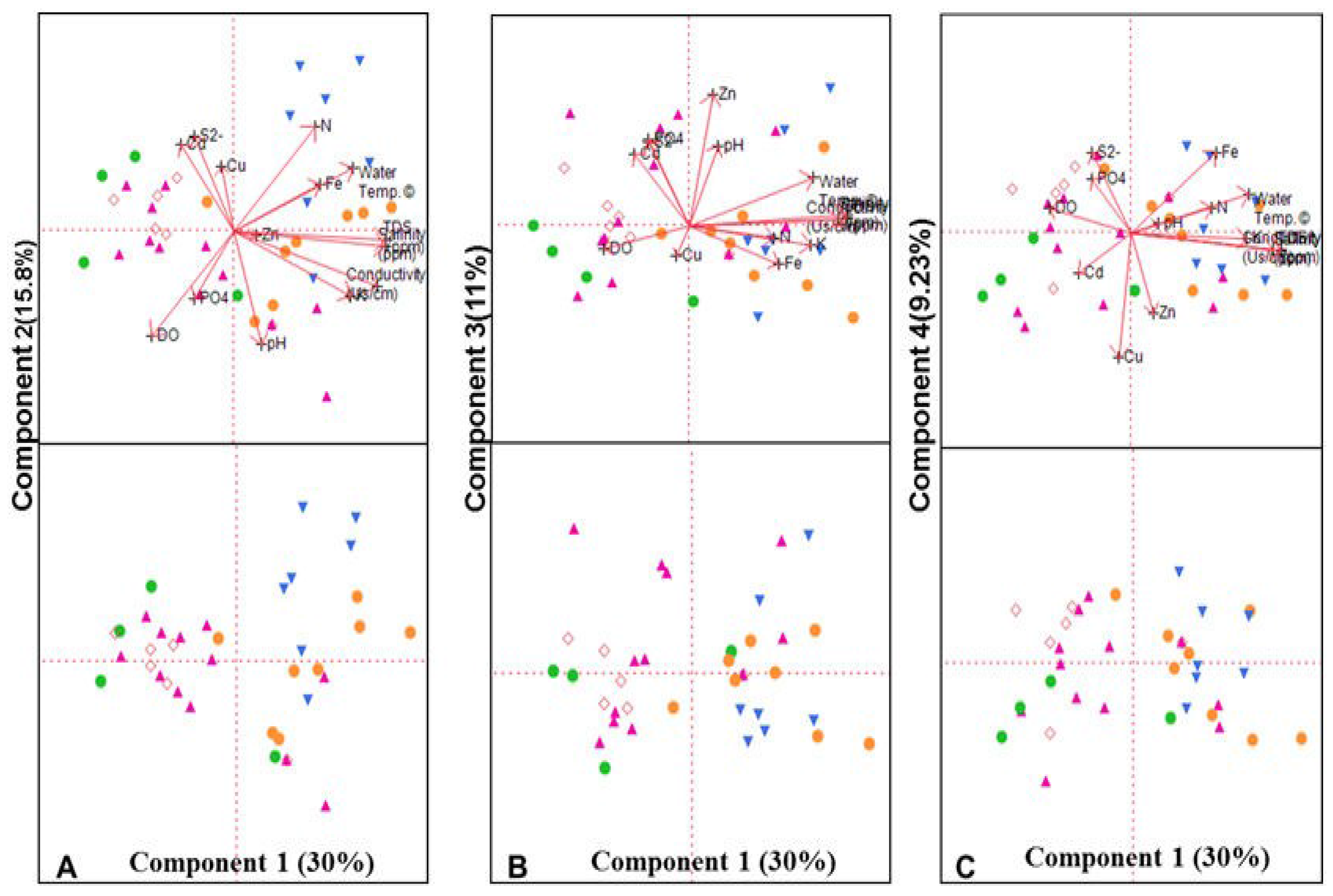
3.2. PCA Results of Water Quality Data from Rivers Sampled in Laikipia and Meru

3.2.1. Principal Components (PCs)

The field raw data consisting of all 14 measured variables for all 38 sites were log transformed to make sure the data follow an approximate normal distribution [46] prior to principal component analysis (PCA). The resulting single matrix consisted of 14 parameter measurements of concentrations (mg/L, EC (µS/cm), pH, water temperature (°C)). The Bartlett’s sphericity adequacy test was performed to test data suitability for PCA. We obtained a significant (p < 0.001) score of 0.69, which was within the recommended range for PCA. A robust PCA was done in SPSS using varimax rotation. The PCA produced four rotated principal components (PCs) that accounted for 70% variance in water quality samples (Table 2).
From the table, the PC1 had strong positive relations with EC, salinity, TDS, and potassium. The variables showing high scores for PC1 (i.e., >0.8) were mainly in sampling points in Meru (Figure 2 and Figure 3).
PC2 has high positive loading with nitrate and water temperature, but negative loading with dissolved oxygen (DO).
Table 2. Results of PCA for all 38 sites located on main rivers in Meru and Laikipia regions. Loadings with absolute values <0.4 were omitted [47,48].
VariablesPC1PC2PC3PC4% Explained Variance
EC0.89 32.34
Salinity0.88 17.01
TDS0.87 11.53
Potassium(K)0.84 8.68
Sulfide (S2−)−0.520.470.42 6.32
Cadmium (Cd)−0.44 −0.436.22
Iron (Fe)0.44 4.91
DO −0.78 3.59
Nitrate (NO3) 0.75 3.37
Water temp. (C°)0.500.73 2.75
Zinc (Zn 2+) 0.77 1.56
pH −0.420.60 0.96
Phosphate (PO43−) 0.58 0.67
Copper (Cu 2+) −0.810.09
Eigen value4.532.381.611.22
Explained variance0.300.180.120.10
Notes: PC denotes rotated principal components. EC is electrical conductivity; DO is dissolved oxygen; Water temp. is water temperature in °C.
The negative relationship between water temperature and DO is a natural occurrence due to decreasing oxygen solubility with increasing water temperature and vice versa.
Zinc and water pH had high loadings for PC3, while phosphate and sulfide showed moderate loadings.
Copper had a strong negative loading for PC4, while cadmium showed a moderate negative loading. Both loadings are heavy metal traces of environmental concern.

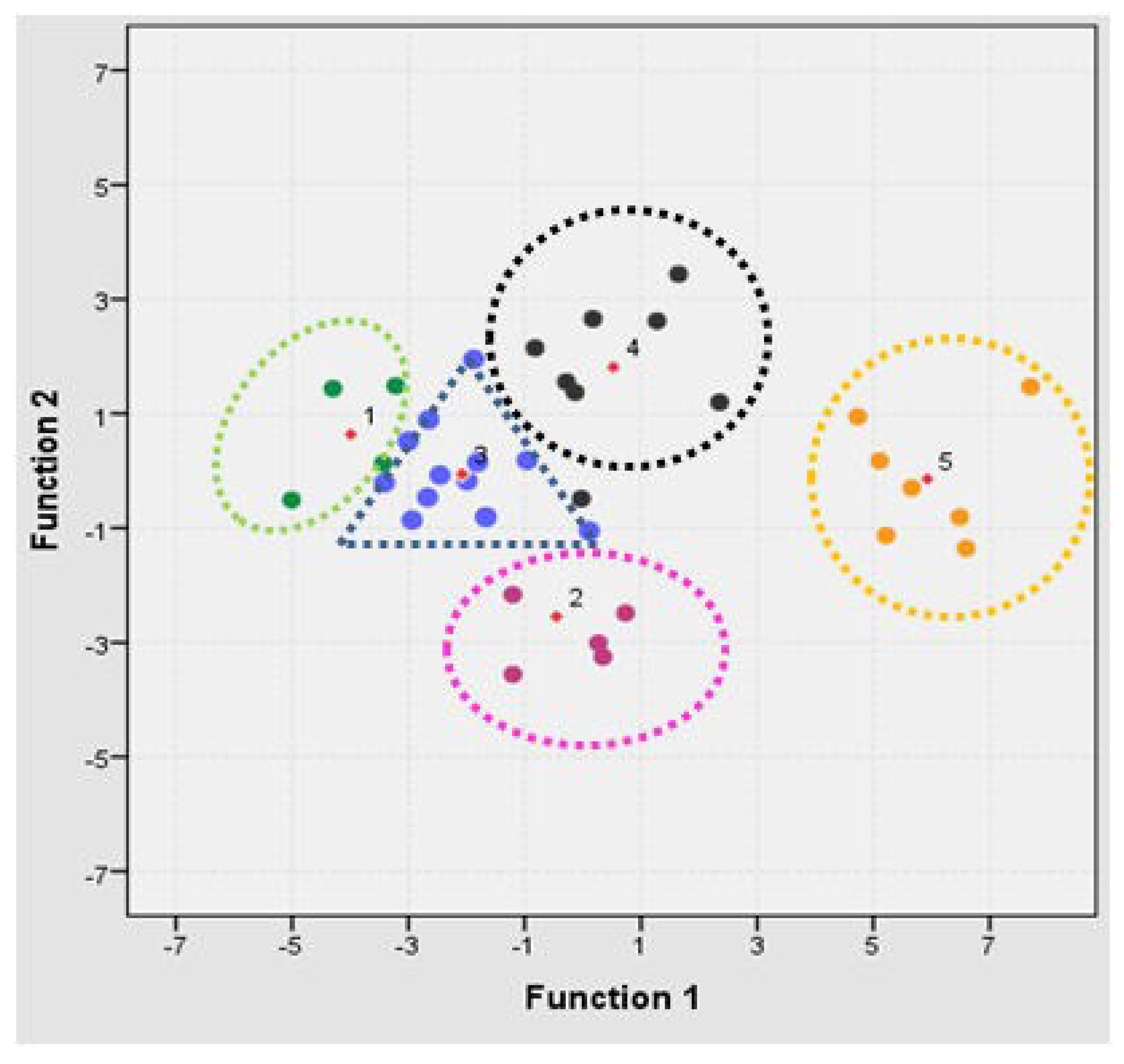
3.2.2. PCA Biplots—Loadings and Scores

The biplots provide a standard tool for investigating and presenting the multivariate data structure based on the overall correlation matrix [40].
Since water quality data is expressed in part per million (mg/L), or milligram/liter (mg/L), it is considered compositional data of multivariate observations [42]. Such data can be displayed in biplots which provide a meaningful way of visualizing the relative information on single compositional parts as well as existing multivariate relationships of parameters [27,41]. The PC scores and loading biplots (Figure 5A–C) show distinctive groups of rays that spread from the origin to different directions, suggesting existing variations in parameters and their magnitudes in the systems.
The symbols represent sites, which are color-coded to represent the five land use types classified (Figure 5 and Figure 6). The rays in the left quadrants identify the dominant parameters in this order: dissolved oxygen (DO) < cadmium (Cd) < sulphide (S2−) < phosphate (PO4) < copper (Cu), where sulphide and DO show longer rays indicative of high variability in the system. The rays in the right quadrants strongly define nitrate, water temperature, salinity, conductivity, potassium, TDS, iron, pH, and zinc.
Figure 5. A group of three biplot panels displaying the PC loadings and component scores. (A) PC1 vs. PC2 explain highest variability in water quality (i.e., 30% and 15.8% respectively); (B) PC1 vs. PC3 illustrate moderate variation (i.e., 30% and 11% respectively); and (C) PC1 vs. PC4 illustrate lowest variation (i.e., 30% and 9.23% respectively). Highly correlating variables form a small angle between the rays and may often overlap, as seen in the right quadrant. Long rays indicate magnitude of the specific variable loading.
Environments 02 00521 g005

3.2.3. Results of Discriminant Analysis (DA)

The main aim of DA was to categorize measured surface water quality parameters into land use types, thereby highlighting potential pollutant source processes. The DA yielded four discriminant functions separating the parameters into five land use groups. A summary table of discriminant function analysis (DFA) statistics is given in Table 3a for all four functions, including the Wilks’ lambda (p < 0.05) test that determines the discriminating capability of the land use groups. The larger the eigenvalue, the more variance shared by the linear combination of variables. The eigenvalues are sorted in descending order of importance, with Functions 1 and 2 explaining great variation in land use type and related water quality characteristic. Discriminant Function 1 significantly accounted for 80.36% of the variability in water quality, while Functions 2, 3, and 4 accounted for 14.59%, 3.61%, and 1.45% of the variability, respectively. From this finding, and as depicted in Figure 6, the surface waters within the MAG, urban, and SSHORT strongly separate/discriminate from the other two land uses based on Function I, implying likely similarities in the type of driving processes. The functions at group centroids showed a clear separation of the land use categories as indicated by the large differences in their group means (Table 3b).
Figure 6. Canonical discriminant functions plot showing different color-coded land use types. Groups 1–5 represent; Environments 02 00521 i001 = Forest; Environments 02 00521 i002 = Urban; Environments 02 00521 i003 = LSHORT; Environments 02 00521 i004 = SSHORT; and Environments 02 00521 i005 = Mixed agriculture land uses respectively.
Environments 02 00521 g006
Table 3a. Summary of discriminant function analysis results.
ResultsFunction 1Function 2Function 3Function 4
Eigen value11.182.030.500.20
% variance80.3614.593.611.45
Canonenical correlation % of variance0.960.820.580.41
Wilks‘ Lambda0.020.180.550.83
Table 3b. Functions at group centroids.
Land Use GroupsFunction
1234
Forest−3.990.64−1.700.04
Urban−0.45−2.550.04−0.53
LSHORT−2.08−0.060.490.40
SSHORT0.521.810.34−0.53
MAG5.93−0.14−0.370.29
Table 3c. Classification results and predicted group membership.
ForestUrbanLSHORTSSHORT MAGTotal
CountForest400004
Urban051006
LSHORT11110013
SSHORT010708
MAG000077
%Forest100.00.00.00.00.0100.0
Urban0.083.316.70.00.0100.0
LSHORT7.77.784.60.00.0100.0
SSHORT0.012.50.087.50.0100.0
MAG0.00.00.00.0100.0100.0
Note: 89.5% of original grouped cases correctly classified.
The classification matrix resulted in 89.5% correct assignment of water quality parameters into corresponding land use categories (Table 3). The values in the diagonal of the table show the correct classification of observations into groups. Land use categories that attain less than 100% predicted group membership imply that the missing percentage was assigned to a different land use group, and are therefore considered a misclassification. Forest and mixed agriculture (MAG) land use groups achieved 100% correct assignations. Small-scale intensive horticulture (SSHORT), large-scale intensive horticulture (LSHORT), and urban land uses received 87.5%, 84.6%, and 83.3% correct assignations, respectively. Some LSHORT sites were misclassified into forest (7.7%) and as urban uses (7.7%), while SSHORT sites (12.5%) were misclassified as urban.

4. Discussion

4.1. Occurrence and Variability of Common Elements in Surface Water

An initial exploratory evaluation of the raw surface water quality data was important in the present study in an effort to understand the prevailing water quality and source processes.

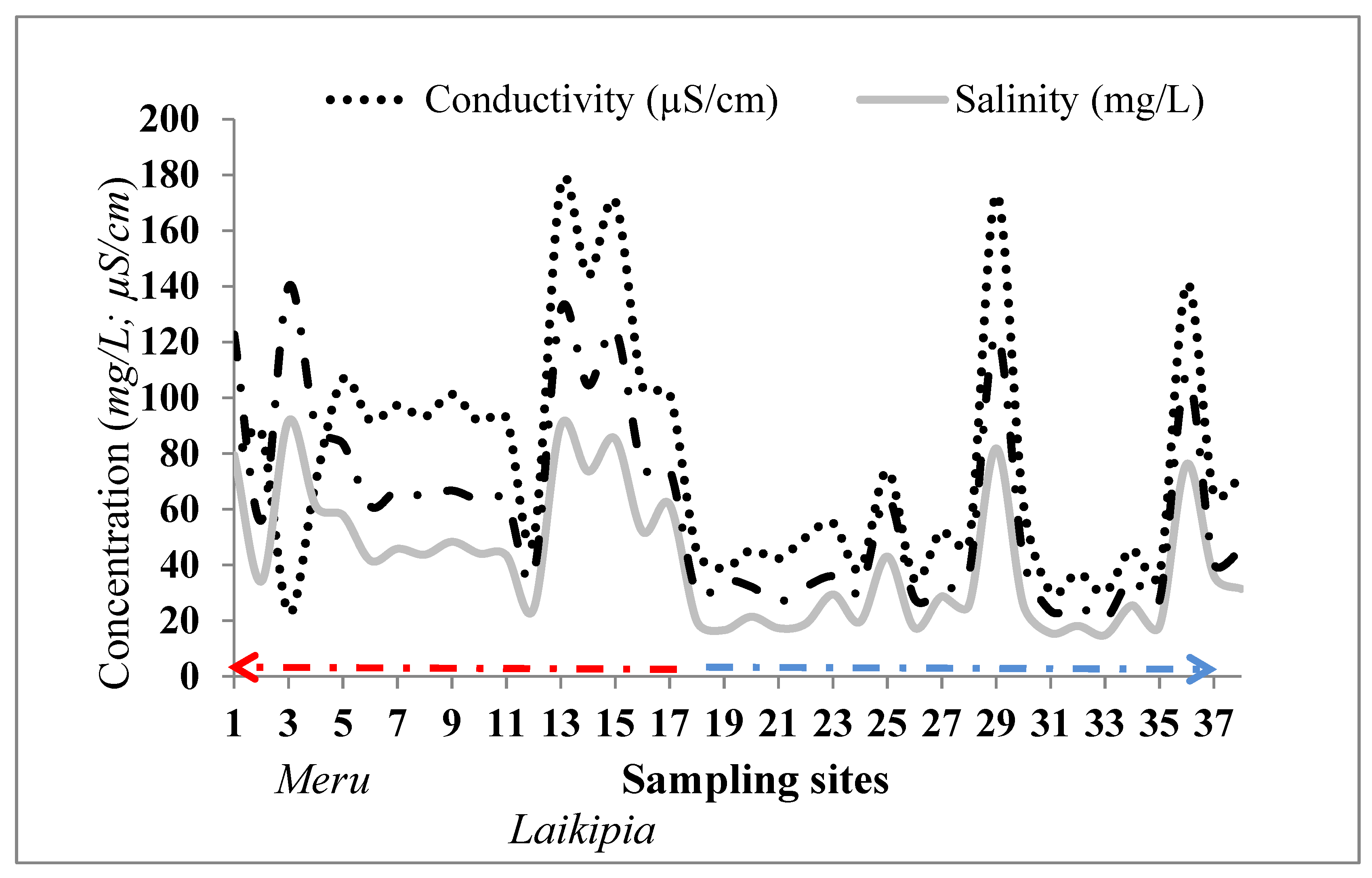
4.1.1. Electrical Conductivity (EC), Total Dissolved Solids (TDS), and Salinity

Our data suggest that EC, TDS, and salinity are highly correlated water quality indicators, central to stream health. These indicators commonly identify processes related to human disturbances such as farming, erosion, and movement of suspended materials and contaminants into rivers [46]. In our analysis, the changes in EC, TDS, and salinity (Figure 2) to high spikes at sites 13, 14, 15, 29, 36 correspond to zones of increased pollutant discharge into river system from adjoining land activities. At sites 13 and 14, snowpea farming by SSHORT intensive farmers was observed, often occurring on stream edges. Farming practices along river banks reduce riparian vegetation buffers, providing an easy pathway for eroding materials into surface waters, affecting water quality. Similar conclusions were drawn by [46], where poor water quality and loss of riparian canopy were negatively correlated with a high concentration of EC, TDS, and salinity. Sites 36 and 29 are located upstream and downstream of large-scale horticulture farms. The ongoing large-scale greenhouse and open-field horticulture activities likely contributed to observed spikes and variability in element concentration. The sudden decline in EC at site 3 was related to a high deposition of fine clay material from upland erosion processes intensified by anthropogenic disturbance. Such a disturbance has implications on the stream bank stability, as it limits stream functionality in sieving/preventing debris entry into the surface waters. The addition of oxygen depleting organic debris, nutrients, and pesticides trigger, significant negative impacts on aquatic ecosystems. This suggests the need for follow-up monitoring, and a management strategy to control runoff and soil erosion by adding cover on riparian zones.

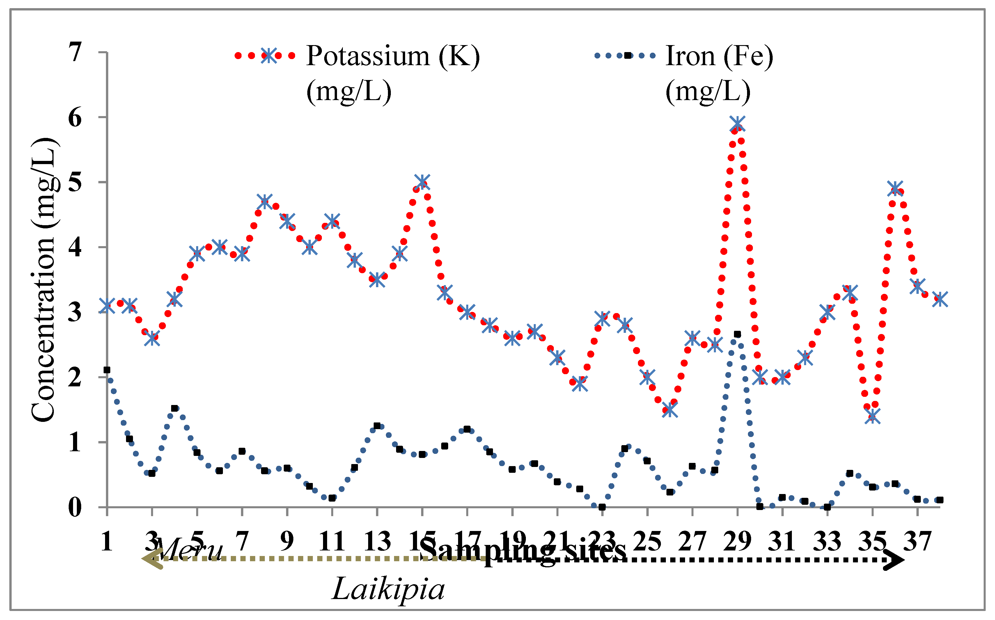
4.1.2. Potassium and Iron

The natural potassium concentration in rivers ranges ~2–3 mg/L, resulting from the weathering of minerals such as feldspars. Higher concentrations of potassium in our study show stronger links to anthropogenic sources than to natural processes. While the potassium concentration presents a smoother curve among sites in Meru, its behavior in Laikipia (sites 18–38) varied greatly, producing a rugged curve (Figure 3). This behavior highlights specific areas where the use of potassium in the surrounding landscape was high, causing spikes in concentration relative to the waters in the same region. The heterogeneous spatial pattern distribution of large-scale greenhouse farming [22] in the sub-watershed may explain the varied potassium peaks in Laikipia where such farming is common. The less noisy potassium concentrations across sites in Meru indicate the consistency of applications by small-scale intensive horticulture (SSHORT) and mixed subsistence agriculture (MAG). Both types of farming are widespread in Meru. The available land parcels are small yet can be turned into productive units under intensive SSHORT, while other farmers maintain tracks of tea farms. Our results (Figure 3) also suggest that the concentration of soluble iron is mainly a function of geological processes. As a matter of fact, kaolinite clays and montmorillonite clays are found in Meru and Laikipia, respectively. These two clays behave differently in water [49,50]. Kaolinite clays could limit the solubility of iron, resulting in low measured levels. On the other hand, montmorillonite clay could enhance the solubility of iron.

4.1.3. Water Temperature, Dissolved Oxygen (DO) and pH

The prevailing temperature differences between the northeast slope (Meru) and the west slope of Mount Kenya (Laikipia) contributed to the observed variation in water temperature and, consequently, the measured DO in the samples. The warmer climatic temperature in Meru directly influenced the water temperature, causing low DO, while in Laikipia, the prevailing cooler temperatures enhanced DO (Figure 4a). The stability of DO in river ecosystems is crucial for the survival of aquatic plants and organisms. Moreover, high temperature and TDS in surface waters leads to lower oxygen solubility. They also concurrently facilitate river eutrophication, particularly in the presence of nitrates [51]. In our study, therefore, the co-occurrence of nitrate (Figure 5A–C), warm waters, and very low DO presents a critical resource management scenario that may accelerate water quality degradation. The use of manure and sludge by SSHORT and MAG farmers as substitutes for synthetic fertilizer is associated with high nitrate concentrations in surface water [52].

4.2. Discussion of Results from Principal Component Analysis (PCA)

4.2.1. Principal Components (PCs)

Up to ~70% variability in surface water quality in the study area was explained by the four PCs (PC1, PC2, PC3, and PC4) (Table 2). The PCs were largely interpreted as processes related to increased commercial horticulture farming and effluent release to surface waters, encroaching farming onto forest lands, vegetation cover reduction, bank instability and erosion, mismanagement of waste streams from coffee factories, automobile repair shops, and urban waste. Geological weathering of underlying bedrock material was also identified as an important process affecting waters in both regions, and contributed to the low iron concentration in Meru water (Figure 3). This interpretation was partially based upon field observation during sampling and site descriptions.
On a scale of 0 to 1, each of the 14 variables (termed as loadings after PCA) scored differently, contributing to the strength of extracted principal components (PC1–PC4). A score close to +1 or −1 by a particular loading indicates a strong influence on the specific PC (Table 2).
PC1 had strong scores from EC, TDS, salinity, and potassium loadings. These processes were mainly associated with increased runoff from on-going SSHORT and MAG uses. The observed peaks in concentration spatially corresponded to areas with intensive commercial horticulture, signaling effluents released into rivers from adjoining landscapes, and hence identifying critical pollution zones.
PC2 had strong positive loading (>0.73) for nitrate and water temperature, and a negative loading for dissolved oxygen (DO). The high nitrate loading was linked to the soaring use of animal manure by both MAG and SSHORT farmers, unlike LSHORT where use of manure is not feasible. The high negative loading for DO shown by the long rays predominantly in the left quadrants (Figure 5A) was associated with cooler headwaters exiting the forests. The mid-zones and lower reaches of the rivers were warmer, presenting important implications for the survival of aquatic ecosystems. Limited stream bank vegetation cover, erosion, cultivation on river banks, and cattle use of the waters are primary factors that significantly degrade the mid-zones and lower waters. Steps towards minimizing such activities can be pursued in an effort to minimize effluent movement.
PC3 had strong to moderate scores from zinc, phosphate, and sulfide loading (Table 2). The strong zinc loading for PC3 can be allied to processes such as the application of phosphate-based fertilizers and agrochemicals, urban effluents from the surrounding town center, car washes and repair stations on the mid-waters of the Nanyuki River in the town of Nanyuki (sites 21, 35), and quarrying activities. Our biplot loadings (rays) for phosphate and sulphide dominate the left quadrant (Figure 5A–C), where the primary land uses are LSHORT and forest. The presence of phosphate across sites indicates its augmented use in the region, with notable spikes in concentration (site 23) (Figure 4b), at sites neighboring on-going LSHORT farming, and sites adjoining tea farming zones (sites 10, 11, and 12 on the headwaters in Meru). Interestingly, sulphide had a moderate loading on PC1, PC2, and PC3, identifying common processes that generate waste effluents into streams. Such processes include industrial waste generated by coffee and tea processing factories in Meru and municipal effluents from residential areas of Nanyuki, and Likii. The common use of pit latrines and poor sanitation systems were also plausible causes explaining observed sulfide traces.
PC4 had a negative moderate loading for cadmium and a high negative loading for copper (Table 2). Both elements are related to phosphate fertilizers, and identify anthropogenic sources of heavy metals and metalloids in surface waters in the region.
While our study presents a one-time sampling event, the obtained information is critical to set discussions on appropriate steps towards managing water resources in the sub-watersheds. Further investigation to examine seasonal variations and flux of parameters into water systems, as well as the integrity of aquatic organisms, may provide more insights into surface systems behavior.

4.2.2. Contributions of Different Land Uses on Stream Water Quality as Revealed by DA

The strength of DA in our study was in its ability to provide a statistical categorization of land use types as sources of pollution. Based on our analysis, the group centroids (Table 3b; Figure 6) provided a better predictive power to the Discriminant Function 1, as seen by the large differences between land use types. Up to 89.5% correct separation of land use types was attained, as shown by the classification matrix. The discriminant results (Table 3c) strongly illustrate the distinct variability in water quality as driven by land use. Similar conclusions were drawn by [53], who argue that significant differences in land use contributed to buildup of Escherichia coli and Enterococci bacteria, and heavy metals in stream waters.

Forest Use and Mixed Agriculture (MAG) Land Use

DA results show that the forest and MAG land use types obtained 100% accuracy in classified water samples. This was supported by a large difference in the forest and MAG group mean (−3.99 and 5.93, respectively, Table 3b) as shown by Function 1. The complete separability of these two land use types by Function 1 is an indication of the underlying variability in surface water quality.
Forest: The headwaters existing in forest use had low temperatures and high DO, which was not unusual. From our findings, the traces of pollutants in waters exiting forest land cover are mainly due to encroaching farming activities and clearing of trees and shrubs on slopes of Mount Kenya (Figure 1).
Mixed agriculture (MAG): MAG was a significant source of nitrate, water temperature, and iron (Figure 5). Soaring fertilizer prices in Kenya prompt subsistence farmers to seek affordable alternatives to crop nutrition [54]. The application of aged dry livestock manure from cattle, goat, and sheep is a common practice among MAG farmers, despite its association with stream water degradation. Even though these types of manures have phosphorous, it is in small amounts compared to nitrogen [55]. Primarily, warmer waters in the MAG land use were attributed to naturally occurring warmer agro-ecological climates. Nonetheless, observed farming along river banks and reduced shade could also exacerbate stream temperatures. Traces of iron (Figure 5) found in samples from MAG were interpreted as resulting from geological weathering of underlying bedrock. The observed high zinc at one site in Meru (site 4 on the Thingithu River) was a result of upstream quarry activity.

Large-Scale Horticulture (LSHORT) Land Use

The LSHORT group mean was −2.08, with 84.6% classification accuracy (Table 3b and Table 3c). A complete separability was not achieved, because two sites were misclassified, one site as belonging to forest and the other to urban uses, due to unclear boundaries between land uses. Besides, large-scale farms are rapidly encroaching on forest edges where access to water by directly tapping the headwaters provides a constant supply of irrigation water. Growth of settlements adjacent to LSHORT farming areas has created urban residential areas, which provide a plausible cause of the misclassification. Linking the DA finding to our earlier analysis, we find dominance of phosphorus, cadmium, copper, and sulphide in samples from the left quadrants (Figure 5A–C) with LSHORT land use, and therefore recognize these elements as important primary pollutants related to LSHORT. This is an important finding because the clustering of commercial companies in the region is ongoing, and poses long-term impacts on stream ecosystems and their health.
Phosphorus promotes bud formation and flowering. It is rigorously used by LSHORT in fertilizer formulations to promote crop development and increase yield. Soluble liquid fertilizers are applied on the plants' foliage or through pressurized drip lines placed near plant roots to enhance uptake. Both methods of application (foliage and soil) are common in horticulture, and of concern due to nutrient leaching and runoff arising during excessive rainfall or frequent irrigation [56]. This provides a realistic explanation to observed traces of phosphorous. Besides, the occurrence of cadmium and copper traces in soils under horticulture land use is highlighted in several literatures [57,58]. The application of copper-based herbicides and fungicides in intensive horticulture is also commonplace [57,59]. This corroborates our finding of copper traces in water samples in LSHORT land use. Horticultural effluents are a global concern, necessitating standards of compliance to regulate the greenhouse horticulture industry. For example, Sweden prohibits greenhouse wastewater disposal into drains, watercourses, or groundwater [60], and in the Netherlands, an effort is underway toward zero nutrient emissions by the year 2027. Under the current situation, we suggest the use of constructed wetlands to collect and treat horticultural wastewaters as a sustainable approach to manage the greenhouse wastewaters. Such wetlands are efficient and relatively inexpensive to construct and operate [61] when land is not limited.

Small-Scale Intensive Horticulture (SSHORT)

The DA results show a high accuracy of classification for SSHORT (87.5% in Table 3c). However, total separability was not achieved due to unclear land use boundaries, where one site was categorized into urban land use. Our findings identify potassium, EC, TDS, and salinity as common indicators of surface waters in SSHORT land use. The domineering use of potassium by SSHORT farmers contributes to the observed little variability in potassium concentration across sites in Meru (Figure 3). Although the weathering of rocks and minerals, and the type of parent rock, may dictate the level of potassium in the water system, our results (Figure 3) exceed the natural range of potassium in rivers (2–3 mg/L). It is plausible that increased SSHORT plays a key role in driving the observed values.
Moreover, intensive farming along river banks reduces the natural riparian buffer, creating the easy movement of eroded materials into surface waters. Such anthropogenic disturbances introduce suspended materials into river system, thereby augmenting the amount of dissolved materials, EC, and salinity of surface waters within SSHORT land use.

Urban Use

The urban land use was highly separable with 83.3% classification accuracy (Table 3c) identifying patterns in water quality associated with urban use. The DA finding supports our earlier highlight identifying sulphide as a major trace element linked to several processes, among them urban waste water effluents. Urban residential areas and suburban settlements have increased in Laikipia, following the rise of commercial horticulture [5,14]. The sudden sprawl has taken a toll on water quality due to the mismanagement of diverse waste streams loaded with pollutants that are swept into surface waters. The anaerobic decomposition of sulphur-containing organic matter, sewage, algae, and industrial wastes from petroleum plants, paper mills, and heavy water plants are recognized as the main anthropogenic sources of sulphide in the environment. Zinc traces in water samples were also likely due to waste dumped from automobile repair shops, and car washes and repair stations in surrounding urban centers.

5. Conclusions

The study findings resonated with an increasing body of literature highlighting the negative implications of intensive horticultural production on aquatic ecosystems. Pollutants from the farms are transported in runoff or through leaching into surface streams and contribute to declining water quality that can limit stream integrity and usefulness. Sub-watersheds experiencing increased commercial horticulture may be more vulnerable to rapid surface water deterioration. The multivariate statistical methods, i.e., principal component analysis (PCA) and discriminant analysis (DA), that were utilized to evaluate the field data enhanced our current understanding of the impacts of increasing horticulture on surface waters in central Kenya. Principal component analysis identified four important principle components that explained 70% of the total variance of the 14 parameters examined in the study. Even though principal component analysis provided a proposition of existing variability in water quality in the study area, it alone was inadequate in providing a statistical approach for determining responsible source processes. Discriminant analysis was effective in separating the heterogeneous samples into five land use groups with high classification accuracy. Based on Discriminant Function 1, forest use and mixed agriculture land use were perfectly separable, while a few misclassifications occurred for large-scale intensive horticulture (two), small-scale intensive horticulture (one), and urban land use (one). This was mainly due to indistinguishable land use boundaries.
Our results show that total dissolved solids, electrical conductivity, and salinity were common in the waters, but increased in concentration at locations with intensive small-scale horticulture and large-scale intensive horticulture. Traces of cadmium, phosphates, and zinc were prevalent in the study area, and highly driven by applications of phosphate-based fertilizers. However, the applications among large-scale intensive horticulture seem intense, frequently prompting the spikes in concentration at sites proximate to such farming. Nitrate was prevalent in small-scale intensive horticulture and mixed agriculture, and linked to the use of farmyard manure. From our results, the relationship between surface water quality and land uses in the sub-watersheds indicates that proliferating commercial horticulture and related activities, e.g., rapid population pressure in a watershed, sprawl of urban areas, and encroachment into forests, has a growing effect towards increasing nutrient loads and other pollutants of environmental concern to surface water.
We recognize that stream waters vary seasonally and diurnally and that several sampling events may provide more representative conditions of the water and land activity. Furthermore, biological assessment of the abundance and diversity of the benthic macro-organisms study component may have been included to obtain a more accurate picture. The study recognizes that a laboratory of the examination of the water samples may have provided a validation to the on-field kit results. However, due to financial strain, time, and the geographical location of the study region (international laws and regulations, and sample movement), a one-time assessment of the physico-chemical characteristics of the rivers was done. Nonetheless, the results reveal interesting patterns that are very significant in watershed management. In a region where no previous works have examined the rivers considered in the study, and in relation to land use processes, our study provides baseline reference data for future investigations and follow-up. Identifying types and sources of pollutants, and how they impact the surface water systems, will help generate discussions on the best management approaches towards sustainable horticulture farming in the region. Currently, the role of stakeholder participation in watershed management in Kenya needs to be strengthened such that the communities sharing the same natural resource base have an equal voice towards figuring what is best for all of them. This effort has been initiated in Laikipia. An integration of water quality management and land use planning in sub-watersheds experiencing a rapid conversion of cover to intensive farming practices can help reduce stream degradation. This can also help reduce the pollution of waters, while promoting the biological integrity of aquatic ecosystems and the protection of human health. Further follow-up investigations are necessary to examine the biological integrity of the river systems, which can provide a longer-term indication of the surface water quality status.

Acknowledgement

We gratefully acknowledge the extensive assistance provided by an undergraduate student, Martin Mwongera, and a local guide (Kimathi Ruteere) while in the field. We also thank Clement Alo for his assistance in providing helpful insights and suggestions on the manuscript.

Author Contributions

The first author designed the study, carried out field work, data analysis and developed the manuscript. The second author did extensive reviews of the methodology, draft organization and editing of the work.

Conflicts of Interest

The authors declare no conflict of interest.

References

  1. Thoen, R.; Jaffee, S.; Dolan, C. Equatorial rose: The Kenyan-European cut flower supply chain. Supply Chain Development in Emerging Markets: Case Studies of Supportive Public Policy; World Bank: Washington, DC, USA, 2000. [Google Scholar]
  2. Dolan, C.; Humphrey, J. Changing governance patterns in the trade in fresh vegetables between Africa and the United Kingdom. Environ. Plan. 2004, 36, 491–509. [Google Scholar] [CrossRef]
  3. Dever, J. Case study #6–5. Small-farm access to high-value horticultural markets in Kenya. In Food Policy for Developing Countries: Case Studies; Cornell University library: Ithaca, NY, USA, 2007. [Google Scholar]
  4. Weinberger, K.; Lumpkin, T.A. Diversification into horticulture and poverty reduction: A research agenda. World Dev. 2007, 35, 1464–1480. [Google Scholar] [CrossRef]
  5. Ulrich, A. Export-oriented horticultural production in Laikipia, Kenya: Assessing the implications for rural livelihoods. Sustainability 2014, 6, 336–347. [Google Scholar] [CrossRef]
  6. Kibichii, S.; Shivoga, W.A.; Muchiri, M.; Miller, S.N. Macroinvertebrate assemblages along a land-use gradient in the upper River Njoro watershed of Lake Nakuru drainage basin, Kenya. Lakes Reservoirs Res. Manag. 2007, 12, 107–117. [Google Scholar] [CrossRef]
  7. Owiti, G.E.; Oswe, I.A. Human impact on Lake ecosystems: The case of Lake Naivasha, Kenya. Afr. J. Aquat. Sci. 2007, 32, 79–88. [Google Scholar] [CrossRef]
  8. Nyakundi, W.O.; Magoma, G.; Ochora, J.; Myende, A.B. A Survey of Pesticide Use and Application Patterns among Farmers: A Case Study from Selected Horticultural Farms in Rift Valley and Central Provinces, Kenya. Available online: http://elearning.jkuat.ac.ke/journals/ojs/index.php/jscp/article/view/744 (accessed on 29 October 2015).
  9. Zhu, W.; Joseph, G.; Karen, S. Land-use impact on water pollution: Elevated pollutant input and reduced pollutant retention. J. Contemp. Water Res. Edu. 2008, 138, 15–21. [Google Scholar] [CrossRef]
  10. West, P.C.; Narisma, G.T.; Barford, C.C.; Kucharik, C.J.; Foley, J.A. An alternative approach for quantifying climate regulation by ecosystems. Front. Ecol. Environ. 2010, 9, 126–133. [Google Scholar] [CrossRef]
  11. Wan, R.; Cai, S.; Li, H.; Yang, G.; Li, Z.; Nie, X. Inferring land use and land cover impact on stream water quality using a bayesian hierarchical modeling approach in the Xitiaoxi River watershed, China. J. Environ. Manag. 2014, 133, 1–11. [Google Scholar] [CrossRef] [PubMed]
  12. Saoke, P. Kenya pops situation report: DDT, pesticides and Polychlorinated Biphenyls. Available online: http://www.ipen.org/ipepweb1/library/ipep_pdf_reports/1ken%20kenya%20country%20situation%20report.pdf (accessed on 29 October 2015).
  13. Kithiia, S.M. Effects of Sediments Loads on Water Quality within the Nairobi River Basins, Kenya. Available online: http://www.ij-ep.org/paperInfo.aspx?ID=85 (accessed on 29 October 2015).
  14. Liniger, H.; Gikonyo, J.; Kiteme, B.; Wiesmann, U. Assessing and managing scarce tropical mountain water resources. Mt. Res. Dev. 2005, 25, 163–173. [Google Scholar] [CrossRef]
  15. Nziguheba, G.; Smolders, E. Inputs of trace elements in agricultural soils via phosphate fertilizers in European countries. Sci. Total Environ. 2008, 390, 53–57. [Google Scholar] [CrossRef] [PubMed]
  16. Magnusson, M.; Heimann, K.; Ridd, M.; Negri, A.P. Pesticide contamination and phytotoxicity of sediment interstitial water to tropical benthic microalgae. Water Res. 2013, 47, 5211–5221. [Google Scholar] [CrossRef] [PubMed]
  17. Arunakumara, K.K.I.U.; Walpola, B.; Yoon, M.H. Current status of heavy metal contamination in Asia’s rice lands. Rev. Environ. Sci. Biotechnol. 2013, 12, 355–377. [Google Scholar] [CrossRef]
  18. Singh, B.P. Nontraditional crop production in Africa for export. In Trends in New Crops and New Uses; ASHS Press: Alexandria, VA, USA, 2011. [Google Scholar]
  19. Otero, N.; Vitòria, L.; Soler, A.; Canals, A. Fertiliser characterisation: Major, trace and rare earth elements. Appl. Geochem. 2005, 20, 1473–1488. [Google Scholar] [CrossRef]
  20. Lugon-Moulin, N.; Ryan, L.; Donini, P.; Rossi, L. Cadmium content of phosphate fertilizers used for tobacco production. Agrono. Sustain. Dev. 2006, 26, 151–155. [Google Scholar] [CrossRef]
  21. Chanda, A.; Akhand, A.; Das, A.; Hazra, S. Cr, Pb and Hg contamination on agricultural soil and paddy grain after irrigation using metropolitan sewage effluent. J. Appl. Environ. Biol. Sci. 2011, 1, 464–469. [Google Scholar]
  22. Justus, F.; Yu, D. Spatial distribution of greenhouse commercial horticulture in Kenya and the role of demographic, infrastructure and topo-edaphic factors. ISPRS Int. J. Geo-Inf. 2014, 3, 274–296. [Google Scholar] [CrossRef]
  23. Vega, M.; Pardo, R.; Barrado, E.; Debán, L. Assessment of seasonal and polluting effects on the quality of river water by exploratory data analysis. Water Res. 1998, 32, 3581–3592. [Google Scholar] [CrossRef]
  24. Tong, S.; Chen, W. Modeling the relationship between land use and surface water quality. J. Environ. Manag. 2002, 66, 377–393. [Google Scholar] [CrossRef]
  25. Bhardwaj, V.; Singh, D.S.; Singh, A.K. Water potential of microorganisms. Acta. Hortic. 2010, 93, 155–167. [Google Scholar]
  26. Arrigo, J.S. Using cooperative water quality data for a holistic understanding of Rivers and streams: Quality of the Chhoti Gandak River using principal component analysis, Ganga Plain, India. J. Earth Syst. Sci. 2011, 119, 117–127. [Google Scholar]
  27. Otero, N.; Tolosana-Delgado, R.; Soler, A.; Pawlowsky-Glahn, V.; Canals, A. Relative vs. Absolute statistical analysis of compositions: A comparative study of surface waters of a Mediterranean River. Water Res. 2005, 39, 1404–1414. [Google Scholar] [CrossRef] [PubMed]
  28. Olsen, R.L.; Chappell, R.W.; Loftis, J.C. Water quality sample collection, data treatment and results presentation for principal components analysis—Literature review and Illinois River Watershed case study. Water Res. 2012, 46, 3110–3122. [Google Scholar] [CrossRef] [PubMed]
  29. Selle, B.; Schwientek, M.; Lischeid, G. Understanding processes governing water quality in catchments using principal component scores. J. Hydrol. 2013, 486, 31–38. [Google Scholar] [CrossRef]
  30. Notter, B. Rainfall-Runoff Modeling of Meso-Scale Catchments in the Upper Ewaso Ng’iro Basin, Kenya. Master’ Thesis, University of Berne, Bern, Switzerland, 2003. [Google Scholar]
  31. Dougall, H.W.; Glover, P.E. On the chemical composition of Themeda Triandra and cynodondactylon. Afr. J. Ecol. 1964, 2, 67–70. [Google Scholar] [CrossRef]
  32. Shisanya, C.A.; Mucheru, M.W.; Mugendi, D.N.; Kung’u, J.B. Effect of organic and inorganic nutrient sources on soil mineral nitrogen and maize yields in Central highlands of Kenya. Soil Tillage Res. 2009, 103, 239–246. [Google Scholar] [CrossRef]
  33. Murage, E.W.; Karanja, N.K.; Smithson, P.C.; Woomer, P.L. Diagnostic indicators of soil quality in productive and non-productive smallholders’ fields of Kenya’s Central highlands. Agric. Ecosyst. Environ. 2000, 79, 1–8. [Google Scholar] [CrossRef]
  34. Okoba, B.O.; Sterk, G. Farmers’ identification of erosion indicators and related erosion damage in the Central highlands of Kenya. CATENA 2006, 65, 292–301. [Google Scholar] [CrossRef]
  35. Gicheru, P.T.; Kiome, R.M. Reconnaissance Soil Survey of Chuka-Nkubu Area. Available online: http://library.wur.nl/isric/fulltext/isricu_i23135_001.pdf (accessed on 29 October 2015).
  36. WRI. World Resources Institute (WRI). Download Kenya GIS Data. Available online: http://www.Wri.Org (accessed on 29 October 2015).
  37. Eyre, B.D.; Pepperell, P. A spatially intensive approach to water quality monitoring in the Rous River catchment, NSW, Australia. J. Environ. Manag. 1999, 56, 97–118. [Google Scholar] [CrossRef]
  38. Wang, X. Integrating water-quality management and land-use planning in a watershed context. J. Environ. Manag. 2001, 61, 25–36. [Google Scholar] [CrossRef] [PubMed]
  39. Geotech. Smart3 Colorimeter Operator’s Manual. 2011. Available online: http://www.geotechenv.com/Manuals/LaMotte_Manuals/smart3_colorimeter_operators_manual.pdf (accessed on 29 October 2015).
  40. Reimann, C.; Filzmoser, P.; Garrett, R.G.; Dutter, R. Statistical Data Analysis Explained: Applied Environmental Statistics with R; Wiley: Hoboken, NJ, USA, 2008. [Google Scholar]
  41. Filzmoser, P.; Hron, K.; Reimann, C. The bivariate statistical analysis of environmental (compositional) data. Sci. Total Environ. 2010, 408, 4230–4238. [Google Scholar] [CrossRef] [PubMed]
  42. Filzmoser, P.; Hron, K.; Reimann, C. Interpretation of multivariate outliers for compositional data. Comput. Geosci. 2012, 39, 77–85. [Google Scholar] [CrossRef]
  43. Shrestha, S.; Futab, K.; Takashi, N. Use of principal component analysis, factor analysis and discriminant analysis to evaluate spatial and temporal variations in water quality of the Mekong River. J. Hydroinform. 2008, 10, 43–56. [Google Scholar] [CrossRef]
  44. Gonçalves, C.; Esteves da Silva, J.C.G.; Alpendurada, M.F. Chemometric interpretation of pesticide occurence in soil samples from an intensive horticulture area in North Portugal. Analytica. Chimica. Acta. 2006, 560, 164–171. [Google Scholar] [CrossRef]
  45. Chambers, J.M.; Cleveland, W.S.; Kleiner, B.; Tukey, P.A. Graphical Methods for Data Analysis; Wadsworth Publishing: Belmont, CA, USA, 1983. [Google Scholar]
  46. Kasangaki, A.; Chapman, L.J.; Balirwa, J. Land use and the ecology of benthic macroinvertebrate assemblages of high-altitude rainforest streams in Uganda. Freshw. Biol. 2008, 53, 681–697. [Google Scholar] [CrossRef]
  47. Hair, J.F.; Anderson, R.E.; Tatham, R.L.; Black, W.C. Multivariate Data Analysis; Prentice Hall: Upper Saddle River, NJ, USA, 1998. [Google Scholar]
  48. Mishra, G.; Ball, K.; Arbuckle, J.; Crawford, D. Dietary patterns of Australian adults and their association with socioeconomic status: Results from the 1995 national nutrition survey. Eur. J. Clin. Nutr. 2002, 56, 687–693. [Google Scholar] [CrossRef] [PubMed]
  49. Palomino, A.; Santamarina, C. Fabric map for kaolinite: Effects of pH and ionic concentration on behavior. Clays Clay Miner. 2005, 53, 211–223. [Google Scholar] [CrossRef]
  50. Rolfe, R.F.; Miller, R.F.; McQueen, I.S. Dispersion Characteristics of Montmorillonite, Kaolinite, and Hike Clays in Waters of Varying Quality, and Their Control with Phosphate Dispersants. Available online: https://pubs.er.usgs.gov/publication/pp (accessed on 29 October 2015).
  51. Razmkhah, H.; Abrishamchi, A.; Torkian, A. Evaluation of spatial and temporal variation in water quality by pattern recognition techniques: A case study on Jajrood River (Tehran, Iran). J. Environ. Manag. 2010, 91, 852–860. [Google Scholar] [CrossRef] [PubMed]
  52. Nyakeya, K.; Raburu, P.O.; Masese, F.O.; Gichuki, J. Assessment of pollution impacts on the ecological integrity of the Kisian and Kisat Rivers in Lake Victoria drainage basin, Kenya. Afr. J. Sci. Technol. 2009, 3, 97–107. [Google Scholar]
  53. 1. Kanga, J.; Lee, S.W.; Cho, K.H.; Ki, S.J.; Cha, S.M.; Kim, J.H. Linking land-use type and stream water quality using spatial data of fecal indicator bacteria and heavy metals in the Yeongsan River Basin. Water Res. 2010, 44, 4143–4157. [Google Scholar] [CrossRef] [PubMed]
  54. Kipkoech, A.K.; Okalebo, J.R.; Kifuko-Koech, M.K.; Ndungu, K.W.; Nekesa, A.O. Assessing Factors Influencing Types, Rate of Application and Timing of Fertilizer Use among Small-Scale Farmers of Western Kenya. Available online: http://repository.ruforum.org/documents/assessing-factors-influencing-types-rate-application-and-timing-fertilizer-use-among-small (accessed on 29 October 2015).
  55. Espinoza, L.; Norman, R.; Salton, N.; Daniels, M. The Nitrogen and Phosphorous Cycle in Soils. Available online: https://www.uaex.edu/publications/pdf/FSA-2148.pdf (accessed on 29 October 2015).
  56. Silberbush, M.; Lieth, J.H. Nitrate and potassium uptake by greenhouse roses (rosa hybrida) along successive flower-cut cycles: A model and its calibration. Sci. Hortic. 2004, 101, 127–141. [Google Scholar] [CrossRef]
  57. Gaw, S.K.; Wilkins, A.L.; Kim, N.D.; Palmer, G.T.; Robinson, P. Trace element and ΣDDT concentrations in horticultural soils from the Tasman, Waikato and Auckland regions of New Zealand. Sci. Total Environ. 2006, 355, 31–47. [Google Scholar] [CrossRef] [PubMed]
  58. Better Farming. Greenhouse Wastewater Discharges Provoke Legislation Debate. Available online: http://www.betterfarming.com/online-news/greenhouse-wastewater-discharges-provoke-legislation-debate 5435 (accessed on 29 October 2015).
  59. Atkinson, J.D.; Chamberlain, E.E.; Dingley, J.M.; Reid, W.H.; Brien, R.M.; Cottier, W.; Jack, H.; Taylor, G.G. Plant protection in New Zealand; New Zealand Department of Education: Wellington, New Zealand, 1956. [Google Scholar]
  60. Alsanius, B.W.; Jung, V.; Hultberg, M.; Khalil, S.; Gustafsson, A.K.; Burleigh, S. Sustainable greenhouse systems—The potential of microorganisms. Acta. Hortic. 2011, 893, 155–167. [Google Scholar] [CrossRef]
  61. Grasselly, D.; Merlin, G.; Sédilot, C.; Vanel, F.; Dufour, G.; Rosso, L. Denitrification of soilless tomato crops run-off water by horizontal subsurface constructed wetlands. Acta. Hortic. 2005, 691, 329–332. [Google Scholar] [CrossRef]

