Detection of Stones in Marine Habitats Combining Simultaneous Hydroacoustic Surveys


Alfred Wegener Institute, Helmholtz Centre for Polar and Marine Research, Wadden Sea Research Station, 25992 List/Sylt, Germany
*
Author to whom correspondence should be addressed.
Geosciences 2018, 8(8), 279; https://doi.org/10.3390/geosciences8080279
Submission received: 18 June 2018
/
Revised: 24 July 2018
/
Accepted: 26 July 2018
/
Published: 28 July 2018
(This article belongs to the Special Issue Geological Seafloor Mapping)
Abstract
:Exposed stones in sandy sublittoral environments are hotspots for marine biodiversity, especially for benthic communities. The detection of single stones is principally possible using sidescan-sonar (SSS) backscatter data. The data resolution has to be high to visualize the acoustic shadows of the stones. Otherwise, stony substrates will not be differentiable from other high backscatter substrates (e.g., gravel). Acquiring adequate sonar data and identifying stones in backscatter images is time consuming because it usually requires visual-manual procedures. To develop a more efficient identification and demarcation procedure of stone fields, sidescan sonar and parametric echo sound data were recorded within the marine protected area of “Sylt Outer Reef” (German Bight, North Sea). The investigated area (~5.900 km2) is characterized by dispersed heterogeneous moraine and marine deposits. Data from parametric sediment echo sounder indicate hyperbolas at the sediment surface in stony areas, which can easily be exported. By combining simultaneous recorded low backscatter data and parametric single beam data, stony grounds were demarcated faster, less complex and reproducible from gravelly substrates indicating similar high backscatter in the SSS data.
1. Introduction
In sublittoral environments, hard substrates like cobbles, boulders, blocks and bedrock provide essential ecosystem functions [1,2]. Especially single stones (cobble, boulders and blocks) in areas where soft substrates dominate, are hotspots for marine biodiversity [3]. For fishes and marine mammals, those areas are important breeding and feeding places [4].
The localization, mapping and documentation of stones in the North Sea (and elsewhere) gains increasing importance since the European Union (EU) implemented the protection of stony areas in the European seas in 1992 [5]. Detailed seafloor information is also a relevant precondition for resource assessments, coastal management and further protection measures. In the German Bight, existing area wide sediment distribution maps [6,7] were interpolated from grab-sample data, which lack resolution and tend to under-represent “coarse sediment” (gravel and stones). Especially stones can hardly be representatively sampled with grab samplers.
Currently, there are no clear definition and consistent demarcation criteria in the international literature for stony areas. Descriptions like “high concentration of stones” [8] or “reef like structures” [9] are very vague and insufficient for habitat classification and modelling according to e.g., EUNIS (European Nature Information System) or HELCOM HUB (HELCOM Underwater Biotope and Habitat System) standards. Standardized demarcation criteria such as the distance between stones and the number of objects on a certain area do not exist. Both approaches require at least the localization of the single stones in adequate resolution. In this context, remote sampling techniques such as trawling, dredging, grab sampling and video inspection are inappropriate.
Sidescan sonar (SSS) imaging is a method to detect differences in material and texture of the seabed as well as to identify objects on the seafloor [10,11,12,13]. In general, coarser sediments (rougher surface) will backscatter more energy than finer sediments (smoother surface) [12]. Elevated objects affect the sonar pulse by causing high backscatter at the front and an acoustic shadow (no backscatter) behind the object. The shadow length is strongly related to the location of the object relative to the sound source (here: the SSS tow fish) and the object height [10]. The geometric relationship between these parameters enables the calculation of object heights. Objects close to the tow fish cast shorter shadows when compared to objects of the same size located farther away. As a result, objects close to the sonar produced a shadow below the sonar data resolution and makes them undetectable. Further limitation in the detection of objects is given by benthos living on it. The biomass may absorb and scatter part of the acoustic signal so that the typical high backscatter at the front of the object does not occur [10]. Therefore, automatic detection of objects like stones in sidescan sonar backscatter data is difficult. It basically works out for objects (e.g., mines) lying on homogeneous backscatter grounds [14]. In principle, manual detection is possible but it requires time and high resolution of backscatter to detect small objects. Moreover, the smaller the objects to be identified, the higher resolved data are necessary and the more time consuming is the data acquisition as the survey speed needs to be reduced in order to fit more pings on a given survey line. If the data resolution is insufficient to show the acoustic shadow, a differentiation from the surrounding sediment is hardly possible.
The use of swath systems like multibeam echo sounder (MBES) for object identification is only known for mine detection [15]. The implementation for area-wide stone detection is not practicable due to the very narrow swath in shallow waters and relative low resolution compared to SSS.
Acoustic ground discrimination systems (AGDS) can be instrumental in the effort to demarcate stony areas [16,17,18]. Aside from the standard single-beam technique that does not allow areawide measurements, the disadvantage of such systems is the relatively large opening angle causing a large foot print (e.g., ~5.2 m at 30 m water depth). A smaller foot print is given by parametric sediment echo sounders (pSES) [19,20]. The nonlinear acoustic propagation generated by pSES provides high vertical resolution (decimeter) data with small footprints (e.g., ~1.0 m at 30 m water depth) at low frequencies (e.g., 12 kHz). This technique has been successfully used for the detection of anthropogenic objects lying on or embedded in the seabed like wrecks or pipelines [19,20,21,22]. Generally, hard objects are indicated in the pSES as hyperbolic curves.
The motivation of this paper is to develop an innovative and novel approach to efficiently and reproducibly identify and demarcate areas of exposed stones (erratic cobble, boulders and blocks) by combining SSS and pSES data. In particular, the goals for this new method are to:
- differentiate zones of high SSS backscatter into:
- (a)
- rippled gravelly seafloor largely without stones
- (b)
- seafloor with exposed stones
- identify stone-bearing areas for further high-resolution investigations
Validation measurements were carried out in the area of the paleo Elbe valley (PEV) and the protected area “Sylt Outer Reef” (SOR) in the German Bight. The working areas include homogeneously distributed sands with single scattered stones on the seafloor and areas with heterogeneous sediment distribution where glacial lag deposits (mixed sediments including stones), gravelly substrate and Holocene fine sands change on small scales.
2. Materials and Methods
2.1. Regional Settings
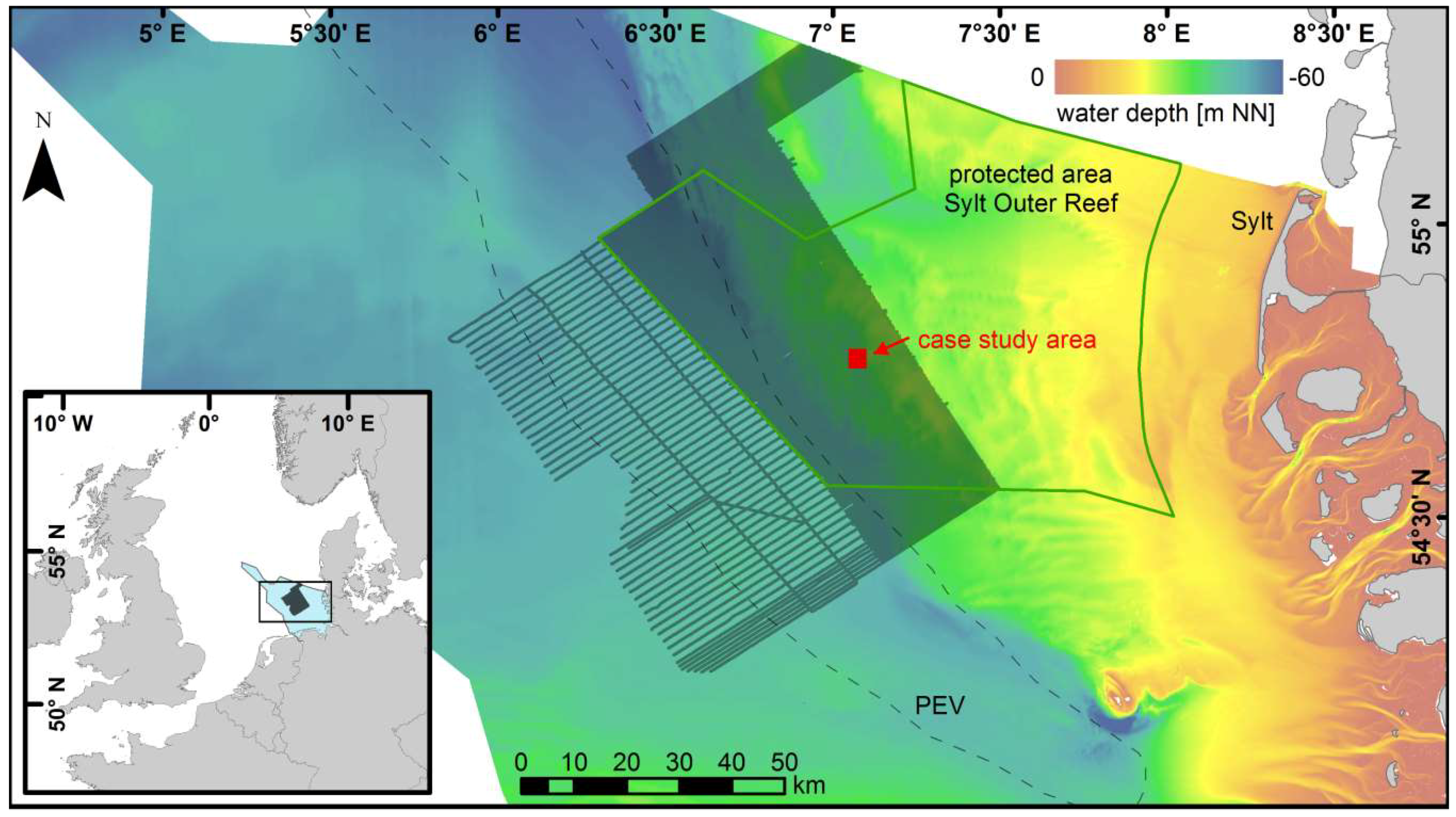
The study site is located in the German Bight, 60–130 km west of the northernmost German island Sylt (Figure 1). Several glacial advances and retreats during the Saalian [23,24] and earlier glaciations shaped the seafloor and left complex sequences of glaciofluvial and glacial deposits e.g., [24,25,26]. During the last glacial phase, the Weichselian (sea level −130 m below present), the German Bight was not covered by ice [24]. At this time the western part of the study area was cut by the paleo Elbe valley (PEV, Figure 1), an approximately 16 m deep and 30–40 km wide valley which discharged large amounts of melt water in north-westerly direction [27,28,29]. The eastern flank of the valley is marked by Pleistocene moraine deposits (including stones up 1.5 m in size) that were exposed to subaerial processes until the sea level rose to 40 m below the present, around 10 ka BP. During the Holocene sea-level transgression, the PEV and the adjacent Pleistocene deposits were submerged. Eventually, the valley filled with Holocene marine sediments [28], whereas part of the moraine deposits is still visible at the seafloor or covered only by a relatively thin layer of sand [30]. As a result homogeneous fine sands characterize the modern sediment surface of the PEV. Heterogeneously distributed fine and coarse sediments mark the SOR [6,7]. However, there is currently no further differentiation of coarse sediments (gravels and stones) in this area.
The seafloor is under permanent influence of near-bed currents which are characterized by semidiurnal tidal cycle and of storm-induced waves which can reach the seafloor in the shallower parts of the study area. The water depth is 20–47 m and bottom slope does not exceed 1°. Nonetheless, earlier SSS monitoring programs in parts of the study area indicated that the sediment distribution pattern especially in the heterogeneous areas is quite stable over time [30].
2.2. Methods
An area of 5900 km2 (Figure 1) was hydroacoustically (SSS, pSES, AGDS), sedimentologically (grab sampler) and optically (underwater video) investigated during four surveys with the German RV Heincke between 2013 and 2015 (see also Table 1). The track orientation was generally set perpendicular to the course of the PEV (NE-SW); the distance of the hydroacoustic profiles was 400 m in areas with heterogeneous sediment distribution and 1600 m in areas with homogeneous sediment distributions (e.g., PEV). An additional hydroacoustic survey was carried out in a small case study area (13 km2) with profiles in north-south and east-west direction and a track distance of 100 m. The survey speed was 5–6 knots during all surveys. Data positioning was accomplished via DGPS (Differential Global Positioning System) (Trimble SPS461).
Data source for seafloor characterization are SSS backscatter images recorded with a towed multi pulse Edgetech 4200-MP. For area-wide mapping, the 300 kHz frequency was used. The swath was set to 460 m in order to obtain a resolution of 1 m along track. The case study area was investigated with a range of 75 m in order to obtain a resolution of 0.25 m along track. Raw data were processed (correction of slant range, speed, layback and gain normalization) using SonarWiz (Chesapeake Technology: California, CA, USA). Stone signatures were manually digitized based on high and low resolution backscatter mosaic of the case study area. Criteria to identify stones were high backscatter at the front and an acoustic shadow (no backscatter) behind the stone. Ground truthing was carried out with grab samples (Van-Veen-Type HELCOM standard) and underwater video inspection (Kongsberg Color Zoom Camera and GOPRO 3+ Black Edition). Back in the home lab grain-size analyses for samples with fractions smaller than 2 mm were carried out with a CILAS 1180 L laser particle sizer (0.04–2500 µm) after chemical treatment according to standard procedures [31]. Sediments with fractions larger than 2 mm were analyzed by wet sieving. The textural classes are according to FOLK [32].
Internal sediment structures as well as objects lying on the sediment surface directly under the ship track were detected using the pSES “SES-2000 medium” (hull mounted) by Innomar Technology GmbH (Rostock, Germany). In comparison to common linear sub-bottom profilers, non-linear systems give an improved signal to noise ratio which results in a high vertical and lateral resolution. The nonlinear interference of two propagating and slightly different frequencies generate a lower, second frequency which corresponds to the differences of the transmitted primary frequencies [19,20]. The secondary frequency has the same narrow beam as the primary frequencies resulting in a small footprint, short pulses and a main lobe with no significant side lobes [19,20]. The horizontal resolution (along track) depends on the footprint which is less than 3.5% of the water depth. In this study the footprint varied between 0.7 and 1.6 m (in comparison: 3.5–8.3 m footprint for linear single beam systems). The ping rate was at 7–10 pps resulting in one ping every 30–40 cm at a survey speed of 6 knots.
The primary (high) frequency is preset to 100 kHz. The secondary (low) frequency was set between 5 and 15 kHz with a pulse length of 1 and 2 to test the detection precision of objects in dependence of the acoustic behavior (see also Table 2). Stone signatures (hyperbolic curves) were manually marked and exported as XY-data using the software ISE by Innomar Technology GmbH.
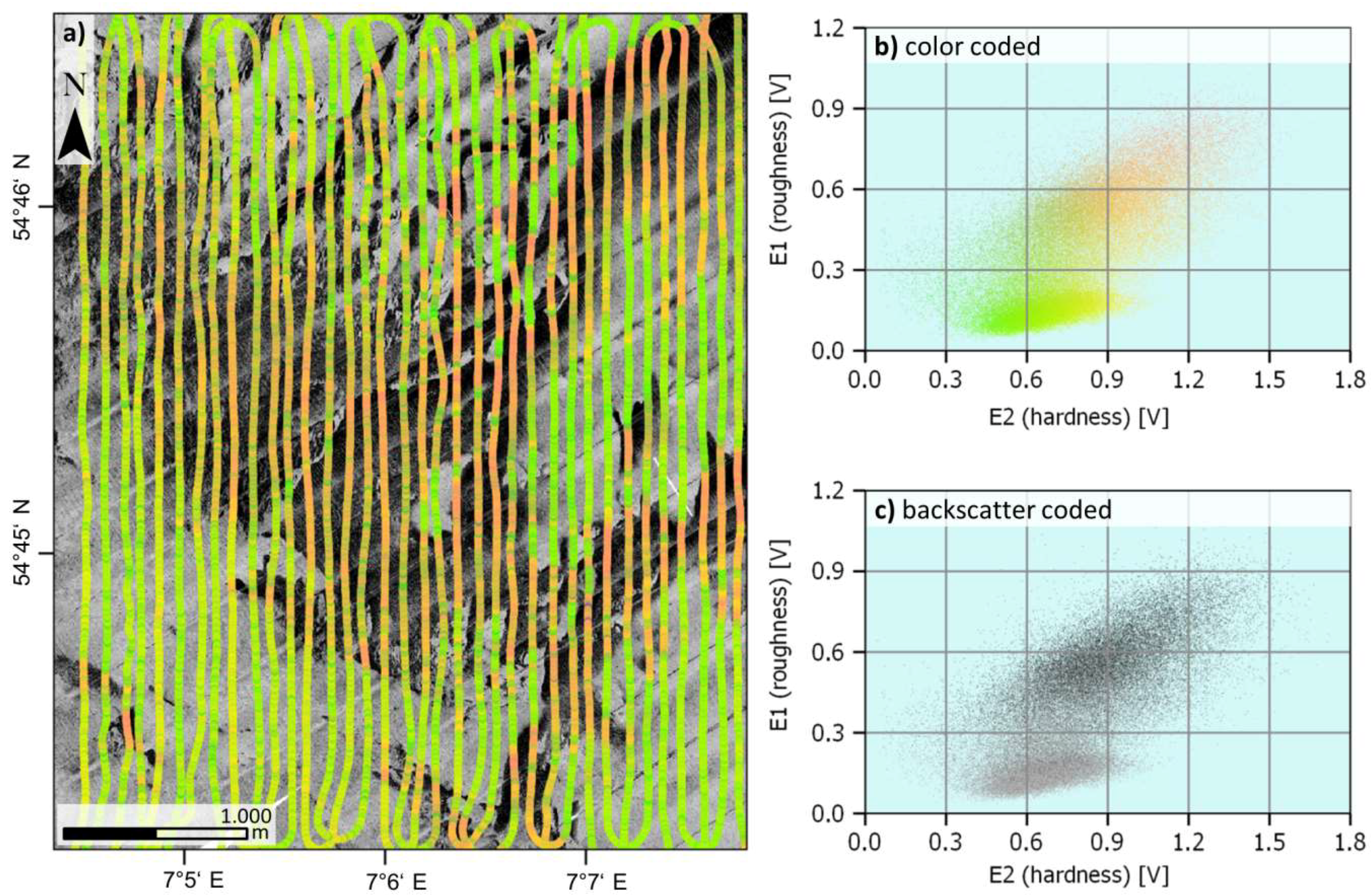
For additional acoustic ground discrimination, the AGDS RoxAnn GD-X (Sonavision Ltd., Aberdeen, UK) together with Furunu 520-5MSD 50/200 kHz dual-frequency transducer and RoxMap acquisition software were used. The frequency was set to 200 kHz with a sampling rate of 1 Hz. The system records the water depth, a specific part of the tail of the first echo return (E1) and the entire second echo (E2). E1 is commonly interpreted as the roughness and E2 as the hardness of the seafloor. The values are given in voltage. For more details see Penrose [33] and Hass et al. [16]. For graphic representation, the E1 and E2 values were plotted in two XY diagrams with different color scales.
- Color coding: according to Hass et al. [16].
- Backscatter coding: AGDS data points are colored in the SSS backscatter gray value that occurred at the point location. This value was extracted from the high resolution SSS mosaic raster with the ArcGIS (Esri Inc., Redlands, CA, USA) spatial analyst tool “Extract values to Point”.
3. Results
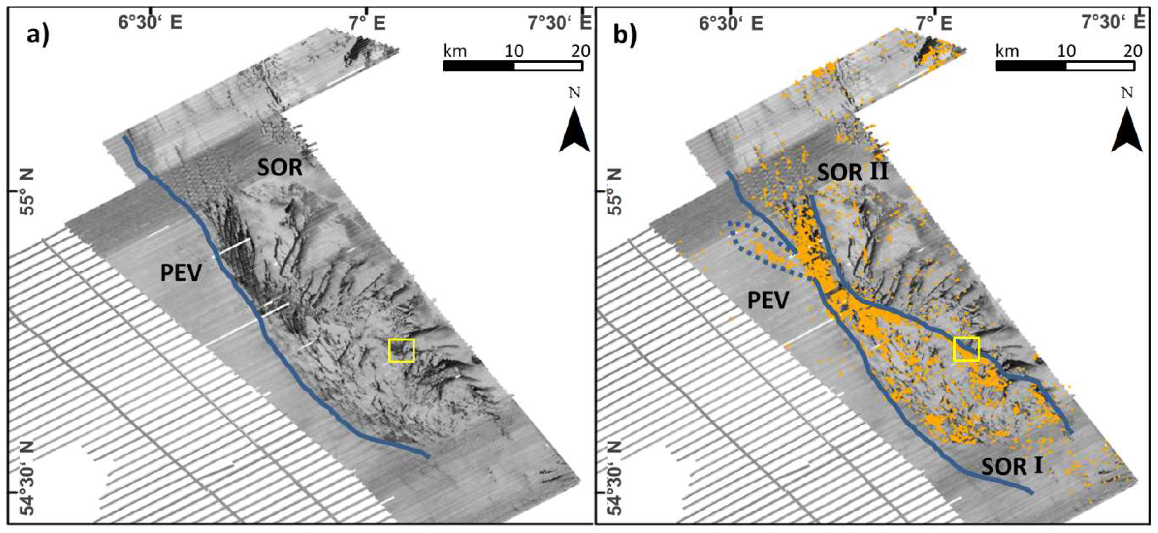
The area-wide, low-resolution SSS backscatter mosaic in combination with the ground-truth data suggest to differentiate the working area into two sedimentologically different areas as shown in Figure 2a:
- the paleo Elbe valley (PEV)
- the Sylt Outer Reef (SOR)
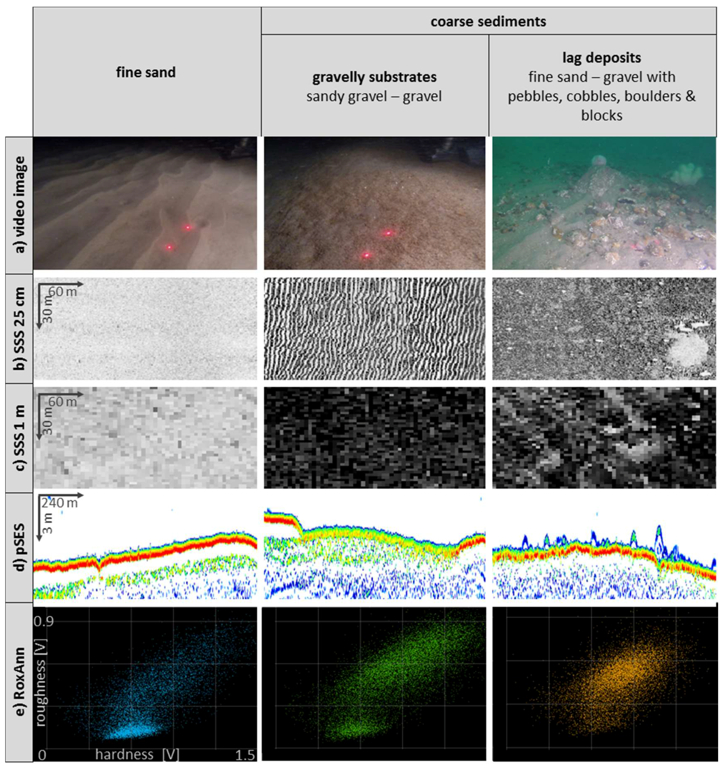
The PEV reveals low backscatter data representing muddy fine sands (mean 100 µm). The SOR located east of the valley shows small-scale changes of high, medium and low backscatter. Low-backscatter data represent fine sands (mean 190 µm) and medium backscatter rippled medium sands (mean 320 µm). High backscatter represents two different coarse sediments (Figure 3):
- lag deposits: poorly sorted sediments with a matrix of fine sand to gravel with pebbles, cobbles, boulders and blocks up 1.5 m in size
- gravelly substrates: large ripples (up to 30 cm in height) of sandy gravel to gravel (described in more detail by Papenmeier et al. [34])
A differentiation of gravelly substrate and lag deposits by means of the backscatter on a larger scale is hardly possible. There are no differences in the backscatter values and typical ripple marks or stone signatures are hardly visible at a spatial resolution of 1 m (Figure 3). In the case study area with a spatial resolution of 0.25 m such signatures are apparent. The amount of stones identified manually from the two SSS mosaics differ significantly (844:11,079) (Figure 4a,b). Generally, the stones were identified on high backscatter data in the central part of the case study area. Almost no stones are present in the northeastern high backscatter area.
The AGDS data suggest a sediment distribution pattern similar to the low resolution SSS backscatter (Figure 5). The E1/E2-scatter plot indicates two clusters: (1) smoother and softer values which corresponds with low SSS-backscatter values (sand); and (2) rougher and harder values which corresponds with high backscatter data (gravelly substrate and lag sediments). Moreover, lag sediments with stones do not produce significantly different AGDS-values compared to rippled sandy gravel to gravel areas (Figure 5c).
In areas with high SSS backscatter, the pSES data sometimes reveal diffracted hyperbolas at the sediment surface (Figure 6). They become best-defined with the following pSES settings: high frequency, small pulse length and a minimum window length (Figure 6c). The position of the diffraction hyperbolas is plotted on top of the SSS backscatter mosaic in Figure 2b and Figure 4c,d. Every hyperbola always represents multiple acoustic pings. Extensive ground truthing data, including high-quality underwater videos, show that these hyperbolas are associated with accumulations of pebbles, cobbles, boulders and blocks occurring together with fine sands to gravel (lag deposits). Locations of the hyperbolas clearly correlate with locations of stone deposits that were identified manually in the backscatter mosaics of the case study area (Figure 4a,b).
4. Discussion
Area-wide mapping of SSS backscatter data showed that the differentiation of lag sediments (containing stones) from gravelly substrate (without stones) is challenging in the area of the SOR, because backscatter values are too similar and typical textures and bedforms were unidentifiable in the 1 m resolution data set. To figure out ecologically important stony areas, further information or high resolution data is needed.
The case study showed that it is principally possible to identify stony areas using SSS data with adequate resolution. However, the effort to manually “click” objects visible to the eye on a computer screen for demarcation purposes is high. It is only feasible for small areas or special investigations such as marine constructional ground investigations and environmental impact assessments. Extrapolating observations from smaller case studies to larger areas is generally impossible [35]. Even studies using a large dataset of sediment sample information often underestimate size classes of gravel and stones [36]. Moreover, earlier studies reported that grab samplers deployed in stony areas mainly catch finer sediment in between stones and are therefore not representative [37,38,39,40]. This has been confirmed during surveys for this study.
Automated object identification for demarcation purposes was not applicable for this data set because stones are always present in areas of mixed sediments which generate a diffused backscatter. So far, quick and automated object identification is only successful when the objects are sitting on homogeneous, low backscatter substrates (e.g., fine sand) [14]. Object identification becomes difficult and even impossible close to the nadir and also when the backscatter is unclear (e.g., stones on mixed sediment). Moreover, noises in the record created by rough sea conditions or by fishes in the water column can produce spots on the record that may be misinterpreted. Even the data acquisition time is almost sixfold for data with a resolution of 0.25 m when compared to one-meter resolution.
The AGDS RoxAnn, originally designed for the fishing industry [41], to distinguish rocks from sand (to save bottom trawls from being destroyed) was indeed able to differentiate between fine and coarse sediments at the SOR. Fine sands with only small ripples have a much smoother surface (lower backscatter) than the large gravelly ripples and the lag deposits with stones (higher backscatter). However, the acoustic properties of the two coarse sediment types are very similar and cannot be differentiated by RoxAnn with certainty. Similar findings were reported by Humborstad et al. [42] who related this deficiency to the relation of size between footprint and hard bottom patches and to the effect of sessile biota on the acoustic characteristics. The substrate patches at the SOR are mostly larger than the footprint due to relative low water depth. That sessile biota affects the acoustic properties of objects such as stones is reasonable by all means. Michaelis et al. [43] have shown that more than 85% of stones in the area of the SOR are colonized to a varying degree by sessile organisms. As a result, the biotic cover may mask stones and make them undetectable by AGDS. Further, RoxAnn cannot clearly distinguish areas with and without stones as the stones of mostly cobble and boulder size are usually much smaller than the footprint (3.5–8 m).
Areas of stone occurrence are clearly apparent in the echogram of the pSES. The elevated surfaces of stones on the seafloor caused the hyperbolas in the pSES data. The incident wave is diffracted at the edges of the stones similar as it is known from manmade structures like pipelines at the sediment surface as described by several authors e.g., [19,20,22,44,45]. Müller and Wunderlich [44] have shown that even objects (pipeline) of 40 cm diameter can be successfully detected due to the optimized signal to noise ratio of pSES. Dybedal and Bøe [46] reported that one single pass over or along the object, in that case a pipeline, is sufficient for accurate detection and positioning. According to a formula for vertical resolution given by Wunderlich et al. [19], objects of even 5 cm elevation can be detected if the pulse length is low and both the secondary frequency and the ping rate are high.
Aside from stones, the number of features that would generate hyperbolas is small in the study area. Pipelines, wrecks, moorings or rebuilt foundations are the only features that tower over the seafloor. These are usually easy to identify as manmade structures because they are normally registered in navigation charts. Geogenic features like eroded substrate (e.g., marine clay horizons or peat) could possibly generate comparable hyperbolas but so far none of these structures have been observed during ground truthing within the study area. Features that do not exist in the German North Sea, but that are potentially able to produce similar signals, include reef building fauna (e.g., Sabellaria) or manganese nodules. Lo Iacono et al. [47] have observed impedance anomalies close to the seafloor that were likely produced by fish schools and seagrass meadows. However, these hyperbolas differ in intensity and geometry from those generated by stones. Generally, the hyperbolas of stones indicate much stronger impedance than those produced by organic material (e.g., seagrass meadows). Unknown is the effect of sessile assemblages attached on stones. Possibly, they attenuate the acoustic wave and cause less clear or intense hyperbolas. According to the high proportion of colonized stones in the study area [43] it has to be expected, however, that most of the hyperbolas are altered. This is not the case, though. Only view diffuse hyperbolas have been observed. The authors assume that the degree of colonization plays a role. For future research it is interesting to investigate the effect of sessile fauna on the hyperbola characteristics and whether the SES approach can also be used to differentiate colonized from barren stones.
The distribution pattern of hyperbola position and manually marked stones reveals a good to perfect match (Figure 4). However, the single beam information by oneself is insufficient to trace each single stone and to discriminate larger areas of stone coverage in high detail, especially in areas with heterogeneous sediment distribution. The information can be enhanced through a narrow grid of profiles at the cost of more ship time. Best demarcation of stony areas will be achieved when simultaneously recorded pSES and SSS will be combined. SSS backscatter data of lower resolution (e.g., 1 m, i.e., greater survey speed, wider transect distances) proved to be sufficient and can reduce time and costs.
In this study, the combination of SSS backscatter and pSES hyperbola occurrence provides a more detailed description of stone occurrence east of the PEV. Here, several authors e.g., [25,28,30,48] described frequent occurrences of lag deposits and single stones. However, intensive mapping using the SSS-pSES approach reveals that the area east of the PEV can be divided in two areas: SOR I is characterized by frequent occurrences of lag deposits and stones whereas in SOR II rippled sandy gravel to gravel deposits largely without stones dominate. As yet, such a discrimination exclusively based on low resolution backscatter data was not possible.
5. Conclusions
Stones located at the seafloor surface provide important ecosystem functions and thus need to be precisely identified and mapped. Hydroacoustic mapping has proven to be an adequate cost-effective way to produce gapless maps but it lacks the ability to distinguish between stony areas and coarse sediments without stones (e.g., gravel). In this context, our study has provided a time efficient and reproducible method to demarcate stony areas in marine environments.
AGDS turned out to be impracticable to demarcate stony areas because the footprint of the linear acoustic propagating system is too large. To meet the optimum cost-effective ratio, we recommend to simultaneously record wide swath, low resolution SSS backscatter data and pSES data. As a result, SSS data provide regional precise maps of coarse sediments (including areas with and without stones) while pSES data provide information on the occurrence of exposed stones along the nadir. The pSES information about stones is not area-wide but it is dense enough to allow for extrapolation from one transect line to the next. The combination of SSS and pSES compensate for individual limitations of the respective instruments, allow a survey speed of 6 kn (or more) and prevent excessive survey and data acquisition time as well as time consuming data processing and manual stone identification. The extraction of stone signals from pSES data is easy and fast and will be automated for future surveys.
Author Contributions
Conceptualization, S.P. and H.C.H.; Methodology, S.P.; Formal Analysis, S.P.; Investigation, S.P. and H.C.H.; Writing-Original Draft Preparation, S.P.; Writing-Review & Editing, H.C.H.; Visualization, S.P.; Funding Acquisition, H.C.H.
Funding
This research was funded by the project AMIN I–III, a research and development cooperation between the Alfred Wegener Institute Helmholtz Centre for Polar and Marine Research and the Federal Maritime and Hydrographic Agency in Hamburg (BSH). It is part of the project SedAWZ coordinated by the BSH and financed by the Federal Agency for Nature Conservation (BfN).
Acknowledgments
We thank the captain and crew of RV Heincke for their support during our research surveys. We thank our student assistants for their help during the survey and data processing.
Conflicts of Interest
The authors declare no conflict of interest.
References
- Sheehan, E.V.; Bridger, D.; Attrill, M.J. The ecosystem service value of living versus dead biogenic reef. Estuar. Coast. Shelf Sci. 2015, 154, 248–254. [Google Scholar] [CrossRef]
- Taylor, R.B. Density, biomass and productivity of animals in four subtidal rocky reef habitats: The importance of small mobile invertebrates. MEPS 1998, 172, 37–51. [Google Scholar] [CrossRef]
- European Commission. Council Directive 92/43/EEC of 21 May 1992 on the Conservation of Natural Habitats and of Wild Fauna and Flora (Habitat Directive). 1992. Available online: https://eur-lex.europa.eu/legal-content/EN/TXT/?uri=celex%3A31992L0043 (accessed on 27 July 2018).
- Coolen, J.W.P.; Bos, O.G.; Glorisu, S.; Lengkeek, W.; Cuperus, J.; van der Weide, B.; Agüera, A. Reefs, sand and reef-like sand: A comparison of the benthic biodiversity of habitats in the Dutch Borkum Reef Grounds. J. Sea Res. 2015, 103, 84–92. [Google Scholar] [CrossRef]
- Von Nordheim, H.; Boedecker, D.; Krause, J.C. Progress in Marine Conservation in Europe; Springer: Berlin/Heidelberg, Germany, 2006; Chapter 6; p. 263. ISBN 978-3-540-33290-9. [Google Scholar]
- Figge, K. Sedimentverteilung in der Deutschen Bucht (Blatt-Nr. 2900, Maßstab 1:250 000); Deutsches Hydrographisches Institut: Hamburg, Germany, 1981. [Google Scholar]
- Laurer, W.-U.; Naumann, M.; Zeiler, M. Erstellung der Karte zur Sedimentverteilung auf dem Meeresboden in der deutschen Nordsee nach der Klassifikation von FIGGE (1981). Available online: https://www.gpdn.de/media/1449 (accessed on 26 July 2018).
- Schwarzer, K.; Diesing, M. Erforschung der FFH-Lebensraumtypen Sandbank und Riff in der AWZ der deutschen Nord- und Ostsee, Abschlussbericht für das FuE-Vorhaben FKZ 802 85 270 (Bundesamt für Naturschutz); Institut für Geowissenschaften, Christian-Albrechts-Universität zu Kiel: Kiel, Germany, 2006; p. 71. [Google Scholar]
- Rachor, E.; Nehmer, P. Erfassung und Bewertung ökologisch wertvoller Lebensräume in der Nordsee, Abschlussbericht für das FuE-Vorahben FKZ 899 85 310 (Bundesamt für Naturschutz); Alfred-Wegener Institut für Polar- und Meeresforschung: Bremerhaven, Germany, 2003; p. 175. [Google Scholar]
- Blondel, P. The Handbook of Sidescan Sonar; Springer Praxis Books—Geophysical Sciences; Springer Science & Business Media: Berlin/Heidelberg, Germany, 2009; 316p, ISBN 978-3-540-42641-7. [Google Scholar]
- BSH. Guideline for Seafloor Mapping in German Marine Waters Using High-Resolution Sonars; No. 7201; BSH: Munich, Germany, 2016; p. 147. [Google Scholar]
- Lurton, X. An Introduction to Underwater Acoustics: Principles and Applications; Springer: London, UK, 2002; p. 680. ISBN 978-3-540-78480-7. [Google Scholar]
- Wille, P.C. Sound Images of the Ocean in Research and Monitoring; Springer: Berlin/Heidelberg, Germany, 2005; 471p, ISBN 978-3540241225. [Google Scholar]
- Blondel, P. Automatic mine detection by textural analysis of COTS sidescan sonar imagery. Int. J. Remote Sens. 2000, 21, 3115–3128. [Google Scholar] [CrossRef]
- Brisette, M.B.; Clarke, J.E. Side scan versus multibeam echosounder object detection: A comparative analysis. Int. Hydrogr. Rev. 1999, 76, 21–34. [Google Scholar]
- Hass, H.C.; Mielck, F.; Fiorentino, D.; Papenmeier, S. Seafloor monitoring west of Helgoland (German Bight, North Sea) using the acoustic ground discrimination system RoxAnn. Geo-Mar. Lett. 2016, 37, 125–136. [Google Scholar] [CrossRef] [Green Version]
- Mielck, F.; Bartsch, I.; Hass, H.C.; Wölfl, A.C.; Bürk, D.; Betzler, C. Predicting spatial kelp abundance in shallow coastal waters using the acoustic ground discrimination system RoxAnn. Estuar. Coast. Shelf Sci. 2014, 143, 1–11. [Google Scholar] [CrossRef] [Green Version]
- Wölfl, A.C.; Lim, C.H.; Hass, H.C.; Lindhorst, S.; Tosonotto, G.; Lettmann, K.A.; Kuhn, G.; Wolff, J.O.; Abele, D. Distribution and characteristics of marine habitats in a subpolar bay based on hydroacoustics and bed shear stress estimates—Potter Cove, King George Island, Antarctica. Geo-Mar. Lett. 2014, 34, 435–446. [Google Scholar] [CrossRef]
- Wunderlich, J.; Müller, S.; Erdmann, S.; Hümbs, P.; Buch, T.; Endler, R. High-Resolution Acoustical Site Exploration in Very Shallow Water—A Case Study; EAGE Near Surface: Palermo, Italy, 2005; pp. 1–4. [Google Scholar]
- Wunderlich, J.; Wendt, G.; Müller, S. High-resolution echo-sounding and detection of embedded archaeological objects with nonlinear sub-bottom profilers. Mar. Geophys. Res. 2005, 26, 123–133. [Google Scholar] [CrossRef]
- Kozaczka, E.; Grelowska, G.; Kozaczka, S.; Szymczak, W. Detection of objects buried in the sea bottom with the use of parametric echosounder. Arch. Acoust. 2013, 38, 99–104. [Google Scholar] [CrossRef]
- Vasudevan, M.; Sivakholundu, K.M.; Venkata Rao, D.; Kathiroli, S. Application of Parametric Acoustics for Shallow-Water Near-Surface Geophysical Investigations. In Proceedings of the OCEANS 2006—Asia Pacific, Singapore, Singapore, 16–19 May 2007; pp. 1–4. [Google Scholar] [CrossRef]
- Ehlers, J.; Grube, A.; Stephan, H.-J.; Wansa, S. Pleistocene Glaciations of North Germany—New Results. In Developments in Quaternary Science; Ehlers, J., Gibbard, P.L., Hughes, P.D., Eds.; Elsevier: Amsterdam, The Netherlands, 2011; Volume 15, pp. 149–162. ISBN 978-0-444-53447-7. [Google Scholar]
- Streif, H. Sedimentary record of Pleistocene and Holocene marine inundations along the North Sea coast of Lower Saxony, Germany. Quat. Int. 2004, 112, 3–28. [Google Scholar] [CrossRef]
- Pratje, O. Die Deutung der Steingründe in der Nordsee als Endmoräne. Dtsch. Hydrogr. Z. 1951, 4, 106–114. [Google Scholar] [CrossRef]
- Woldstedt, P. Saalezeit, Warthestadium und Weichseleiszeit in Norddeutschland. E&G Quat. Sci. J. 1954, 4, 34–48. [Google Scholar]
- Behre, K.-E. A new Holocene sea-level curve for the southern North Sea. Boreas 2007, 36, 82–102. [Google Scholar] [CrossRef]
- Figge, K. Das Elbe-Urstromtal im Bereich der Deutschen Bucht (Nordsee). E&G Quat. Sci. J. 1980, 30, 203–211. [Google Scholar]
- Konradi, P.B. Biostratigraphy and environment of the Holocene marine transgression in the Heligoland Channel, North Sea. Bull. Geol. Soc. Den. 2000, 47, 71–79. [Google Scholar]
- Diesing, M.; Schwarzer, K. Identification of submarine hard-bottom substrates in the German North Sea and Baltic Sea EEZ with high-resolution acoustic seafloor imaging. In Progress in Marine Conservation in Europe, 1st ed.; Von Nordheim, H., Boedeker, D., Krause, J.C., Eds.; Springer: Berlin/Heidelberg, Germany, 2006; Chapter 6; pp. 111–112. ISBN 978-3-540-33290-9. [Google Scholar]
- Hass, H.C.; Kuhn, G.; Monien, P.; Brumsack, H.J.; Forwick, M. Climate fluctuations during the past two millennia as recorded in sediments from Maxwell Bay, South Shetland Islands, West Antarctica. Geol. Soc. Lond. Spec. Publ. 2010, 344, 243–260. [Google Scholar] [CrossRef]
- Folk, R.L. The distinction between grain size and mineral composition in sedimentary-rock nomenclature. J. Geol. 1954, 62, 344–359. [Google Scholar] [CrossRef]
- Penrose, J.D.; Siwabessy, P.J.W.; Gavrilov, A.; Parnum, I.; Hamilton, L.J.; Bickers, A.; Brooke, B.; Ryan, D.A.; Kennedy, P. Acoustic Techniques for Seabed Classification; Technical Report; CRC for Coastal Zone Estuary and Waterway Management: Queensland, Australia, 2005; Volume 32, pp. 1–130. [Google Scholar]
- Papenmeier, S.; Galvez, D.; Günther, C.-P.; Pesch, R.; Propp, C.; Hass, H.C.; Schuchardt, B.; Zeiler, M. Winnowed gravel lag deposits between sandbanks in the German North Sea. In Seafloor Geomorphology as Benthic Habitat, GeoHab Atlas of Seafloor Geomorphic Features and Benthic Habitats, 2nd ed.; Harris, P.T., Baker, E.K., Eds.; Elsevier: New York, NY, USA, in press.
- Holland, K.T.; Elmore, P.A. A review of heterogeneous sediments in coastal environments. Earth Sci. Rev. 2008, 89, 116–134. [Google Scholar] [CrossRef]
- Fiorentino, D.; Pesch, R.; Guenther, C.-P.; Gutow, L.; Holstein, J.; Dannheim, J.; Ebbe, B.; Bildstein, T.; Schroeder, W.; Schuchardt, B.; et al. A ’fuzzy clustering‘ approach to conceptual confusion: How to classify natural ecological associations. Mar. Ecol. Prog. Sers. 2017, 584, 17–30. [Google Scholar] [CrossRef]
- Beisiegel, K.; Darr, A.; Gogina, M.; Zettler, M.L. Benefits and shortcomings of non-destructive benthic imagery for monitoring hard-bottom habitats. Mar. Pollut. Bull. 2017, 121, 5–15. [Google Scholar] [CrossRef] [PubMed]
- Eleftheriou, A.; Moore, D.C. Macrofauna techniques. In Methods for the Study of Marine Benthos, 4th ed.; Eleftheriou, A., Ed.; Willey Blackwell: Oxford UK, 2013; pp. 175–251. ISBN 9780470670866. [Google Scholar]
- Jamieson, A.J.; Boorman, B.; Jones, D.O.B. Deep-sea benthic sampling. In Methods for the Study of Marine Benthos, 4th ed.; Eleftheriou, A., Ed.; Willey Blackwell: Oxford, UK, 2013; pp. 285–347. ISBN 9780470670866. [Google Scholar]
- Rees, H.L. Guidelines for the Study of the Epibenthos of Subtidal Environments; ICES Techniques in Marine Environmental Sciences: No. 42; ICES: Copenhagen, Denmark, 2009; p. 90. ISBN 978-87-7482-045-1. [Google Scholar]
- Hamilton, L.J. Acoustic Seabed Classification Systems; Defence Science and Technology Organization, Victoria (Australia), Aeronautical and Maritime Research Lab, No. DSTO-TN-0401; National Library of Australia: Canberra, Australia, 2001.
- Humborstad, O.-B.; Nøttestad, L.; Løkkeborg, S.; Rapp, H.T. RoxAnn bottom classification system, sidescan sonar and video-sledge: Spatial resolution and their use in assessing trawling impacts. ICES J. Mar. Sci. 2004, 61, 53–63. [Google Scholar] [CrossRef]
- Michaelis, R.; Hass, H.C.; Mielck, F.; Papenmeier, S.; Sander, L.; Ebbe, B.; Gutow, L.; Wiltshire, K.H. Hard-substrate habitats in the German Bight (south-eastern North Sea) observed using drift videos. J. Sea Res. 2018, under review.
- Müller, S.; Wunderlich, J. Detection of embedded objects using parametric sub-bottom profiler. Int. Hydrogr. Rev. 2003, 4, 76–82. [Google Scholar]
- Von Deimling, J.S.; Held, P.; Feldens, P.; Wilken, D. Effects of using inclined parametric echosounding on sub-bottom acoustic imaging and advances in buried object detection. Geo-Mar. Lett. 2016, 36, 113–119. [Google Scholar] [CrossRef] [Green Version]
- Dybedal, J.; Bøe, R. Ultra high resolution sub-bottom profiling for detection of thin layers and objects. In Proceedings of the OCEANS ‘94. ‘Oceans Engineering for Today’s Technology and Tomorrow’s Preservation’, Brest, France, 13–16 September 1994. [Google Scholar] [CrossRef]
- Lo Iacono, C.; Mateo, M.A.; Gràcia, E.; Guasch, L.; Carbonell, R.; Serrano, L.; Serrano, O.; Danobeitia, J. Very high-resolution seismo-acoustic imaging of seagrass meadows (Mediterranean Sea): Implications for carbon sink estimates. Geophys. Res. Lett. 2008, 35. [Google Scholar] [CrossRef] [Green Version]
- Diesing, M.; Kubicki, A.; Winter, C.; Schwarzer, K. Decadal scale stability of sorted bedforms, German Bight, southeastern North Sea. Cont. Shelf Res. 2006, 26, 902–916. [Google Scholar] [CrossRef]
Figure 1.
Map of the German Bight showing hydroacoustically covered area (black). The paleo Elbe valley (PEV) is crossing the study area (dashed line, modified after Behre [27]). The bathymetric data set is provided by the Federal Maritime and Hydrographic Agency of Germany.
Figure 1.
Map of the German Bight showing hydroacoustically covered area (black). The paleo Elbe valley (PEV) is crossing the study area (dashed line, modified after Behre [27]). The bathymetric data set is provided by the Federal Maritime and Hydrographic Agency of Germany.

Figure 2.
(a) Backscatter mosaic showing two sedimentologically different areas: “PEV” (paleo Elbe valley) with homogeneously distributed muddy fine sands and “SOR” (Sylt Outer Reef) with small-scale changes of fine sands and coarse sediments. Yellow box shows the location of the case study area. (b) Backscatter mosaic with positions of hyperbolas retrieved from the parametric sediment echo sounder data. Based on that, the SOR can be divided in a more stony (SOR I) and a more gravelly (SOR II) area.

Figure 3.
Main sediment types found in the study area: fine sand, gravelly substrate, lag deposits. For each class, the following supplementary information is provided exemplary: (a) underwater video image (the red laser dots have a spacing of 10 cm), (b) sidescan sonar (SSS) backscatter image in high (25 cm) and (c) low (1 m) resolution, (d) a pSES and (e) the RoxAnn scatter plot.

Figure 4.
Stone observations using different techniques: (a) manually tagged on the low resolution SSS backscatter mosaic, (b) manually tagged on the high resolution SSS backscatter mosaic, (c) hyperbola extraction from pSES survey with track distance of 400 m (NE-SW), (d) hyperbola extraction pSES survey with track distance of 100 m (N-S and E-W). Dark colors in the SSS mosaic represent high backscatter and bright colors low backscatter values.
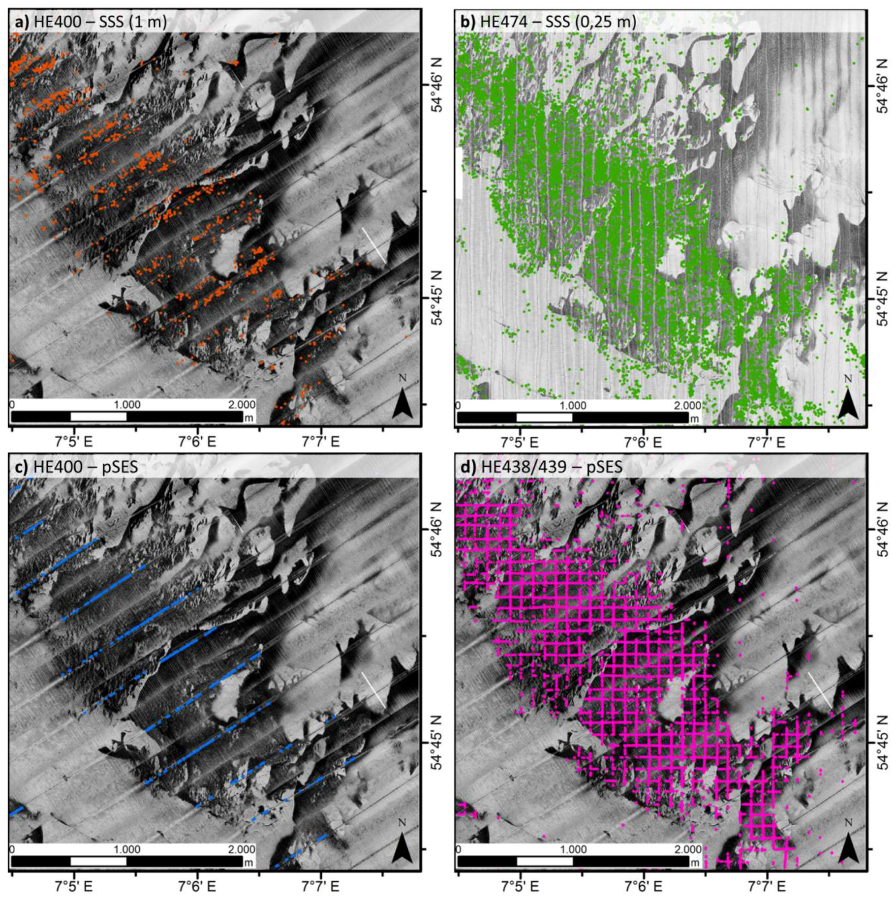
Figure 5.
(a) Low resolution SSS backscatter mosaic (1 m, high backscatter is dark colored) with acoustic ground discrimination systems (AGDS) RoxAnn track color-coded according to (b). (b) RoxAnn E1/E2 diagram. (c) E1 and E2 values colored in the corresponding SSS backscatter gray values. Two classes are suggested: light gray = lower E1/E2 values and dark gray = higher E1/E2 values.

Figure 6.
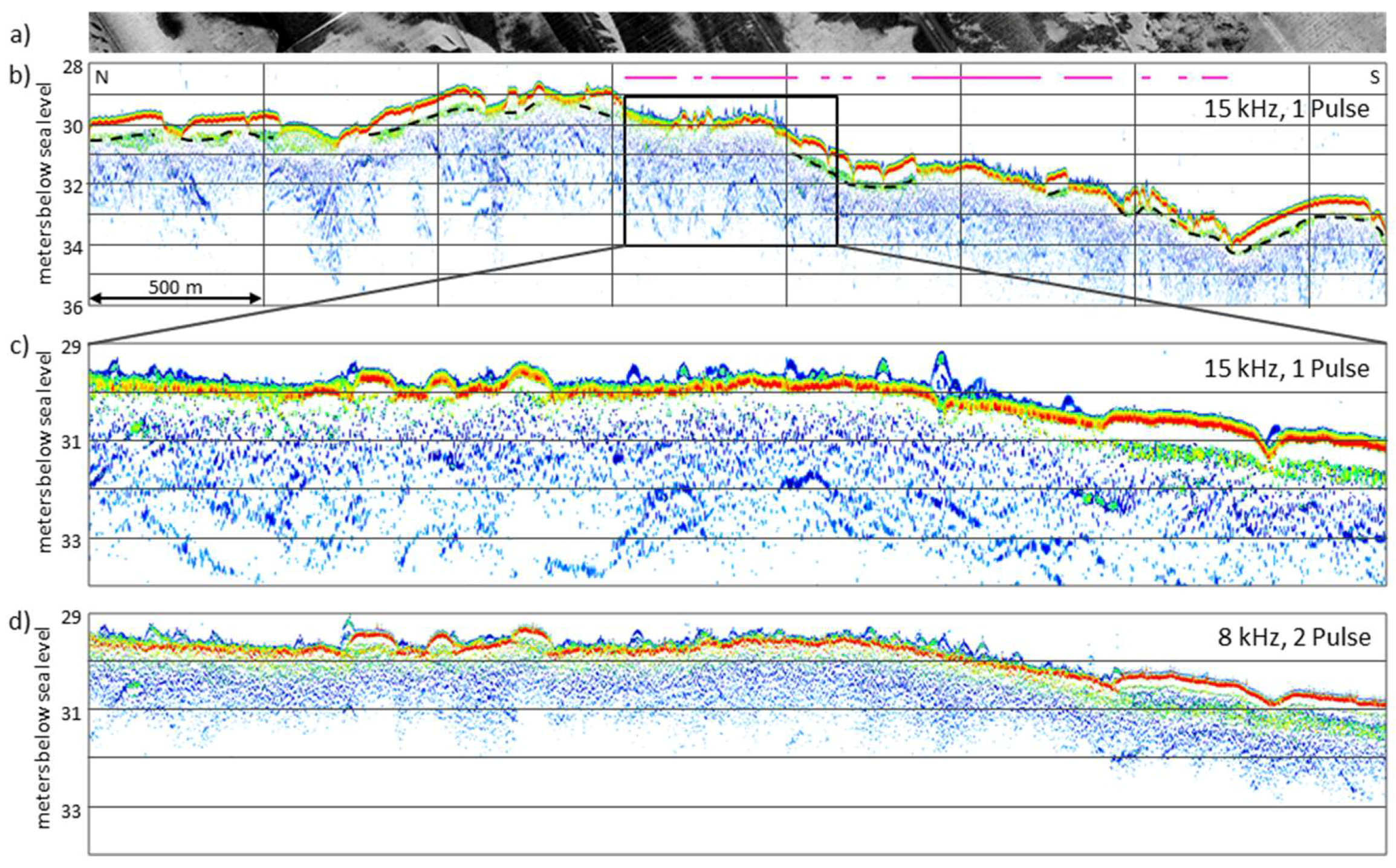
Exemplary pSES profile (15 kHz, 1 pulse) crossing the case study area from North to South (b) with corresponding sidescan backscatter data (a). Low sidescan backscatter data (e.g., fine sands) are represented by greyish colors and high backscatter (e.g., coarse grained sediments) by darker colors. Sediment echo sounder data indicate that coarse sediments are partly covered by fine sands. The boundary between the two facies is marked by the dashed line in (b). The purple lines mark areas with hyperbolas. (c) Zoom of (b). (d) Same section as c recorded with 8 kHz and 2 pulses.
Figure 6.
Exemplary pSES profile (15 kHz, 1 pulse) crossing the case study area from North to South (b) with corresponding sidescan backscatter data (a). Low sidescan backscatter data (e.g., fine sands) are represented by greyish colors and high backscatter (e.g., coarse grained sediments) by darker colors. Sediment echo sounder data indicate that coarse sediments are partly covered by fine sands. The boundary between the two facies is marked by the dashed line in (b). The purple lines mark areas with hyperbolas. (c) Zoom of (b). (d) Same section as c recorded with 8 kHz and 2 pulses.


Table 1.
List of cruises with RV Heincke between 2013 and 2015 and the corresponding parametric sediment echo sounder settings (pSES).
Table 1.
List of cruises with RV Heincke between 2013 and 2015 and the corresponding parametric sediment echo sounder settings (pSES).
| Cruise | Time | pSES Frequency | pSES Pulse Length |
|---|---|---|---|
| HE400 | May 2013 | 6 kHz | 2 |
| HE415 | February 2014 | 10 kHz | 2 |
| HE436 | November 2014 | 8 kHz | 2 |
| HE438/439 | February/March 2015 | 8, 15 kHz | 1, 2 |
Table 2.
Vertical resolution of the parametric sediment echo sound in dependence on frequency and pulse duration. Settings used in the case study area are underlined. The vertical resolution was calculated according to Wunderlich et al. [19]. The speed of sound in seawater was set to 1500 m/s.
Table 2.
Vertical resolution of the parametric sediment echo sound in dependence on frequency and pulse duration. Settings used in the case study area are underlined. The vertical resolution was calculated according to Wunderlich et al. [19]. The speed of sound in seawater was set to 1500 m/s.
| Frequency | Pulse Length | |
|---|---|---|
| 1 | 2 | |
| 6 kHz | 12.5 cm | 25 cm |
| 8 kHz | 9.4 cm | 18.8 cm |
| 10 kHz | 7.5 cm | 15 cm |
| 15 kHz | 5 cm | 10 cm |
© 2018 by the authors. Licensee MDPI, Basel, Switzerland. This article is an open access article distributed under the terms and conditions of the Creative Commons Attribution (CC BY) license (http://creativecommons.org/licenses/by/4.0/).
Share and Cite
MDPI and ACS Style
Papenmeier, S.; Hass, H.C. Detection of Stones in Marine Habitats Combining Simultaneous Hydroacoustic Surveys. Geosciences 2018, 8, 279. https://doi.org/10.3390/geosciences8080279
AMA Style
Papenmeier S, Hass HC. Detection of Stones in Marine Habitats Combining Simultaneous Hydroacoustic Surveys. Geosciences. 2018; 8(8):279. https://doi.org/10.3390/geosciences8080279
Chicago/Turabian StylePapenmeier, Svenja, and H. Christian Hass. 2018. "Detection of Stones in Marine Habitats Combining Simultaneous Hydroacoustic Surveys" Geosciences 8, no. 8: 279. https://doi.org/10.3390/geosciences8080279
Note that from the first issue of 2016, this journal uses article numbers instead of page numbers. See further details here.