GIS and Remote-Sensing Application in Archaeological Site Mapping in the Awsard Area (Morocco)


1
Geosciences Laboratory, University Hassan II, B.P. 3366 Maarif, Casablanca 20100, Morocco
2
Institut National de Sciences de l’Archéologie et du Patrimoine (INSAP), B.P. 6828, Rabat 10000, Morocco
3
Regional Centre for Mapping of Resources for Development, P.O. Box 632-00618, Nairobi 00100, Kenya
*
Author to whom correspondence should be addressed.
Geosciences 2018, 8(6), 207; https://doi.org/10.3390/geosciences8060207
Submission received: 2 April 2018
/
Revised: 14 May 2018
/
Accepted: 15 May 2018
/
Published: 7 June 2018
(This article belongs to the Special Issue Earth Observation, Remote Sensing and Geoscientific Ground Investigations for Archaeological and Heritage Research)
Abstract
:Morocco is famous as one of the archaeologically richest places with many sites. In addition, some of the sites have been listed as UNESCO World Human Heritage sites. In situ observations are used in cultural heritage and archaeological sites mapping. However, this procedure requires periodic observations, which are practically difficult to combine with traditional methods and practices since this is time consuming and expensive. Thus, modern technologies, mainly GIS and remote sensing, are gaining attention as tools for prediction at archaeological sites. The aim of this paper is to assess the application of GIS and remote sensing in order to develop a predictive model, which will be used in locating areas with high potential as archaeological sites in the Awsard area (southern Morocco). The analytic hierarchy process (AHP) as a multi-criteria decision making method, which integrates archaeological data and environmental factors, geospatial analysis and predictive modelling, has been applied to the identification of possible tumuli locations in the study area. The model was developed using a zone of 21 km2 with 233 known sites. It was later validated using 530 unknown sites within an area of 980 km2. The acceptable accuracy of 93% was calculated using an estimation of predictive gain, which proves the efficiency of the model’s predictive ability.
1. Introduction
Morocco is full of archaeological remains, from Volubilis and Lixus (ancient roman cities ruins) in the north of the country to funerary mounds, rocks engravings, and pottery across the country especially in the Moroccan Sahara [1,2,3,4]. The pre-historic funerary monuments (tumuli) are a primary target for looting, since they are known to contain valuable objects. A large part of these monuments have been vandalised by vandals. A general survey should be undertaken in order to effectively protect and study the archaeological sites in the Awsard area. The study of tumuli in Morocco shows that the major groups are located south of the Atlas and the eastern zones in pre-Saharan zones. These tumuli constitute the cultural and environmental diversity of the landscape characterized by large sandy plains located between the Moroccan Saharan desert, the Atlas mountains and the Atlantic coast [5].
Remote sensing has opened up new horizons and possibilities for archaeology. Satellite application in archaeology is an emerging field that uses high-resolution satellites with thermal and infrared capabilities to pinpoint potential sites of interest on the Earth around a meter or so in depth. Satellite remote-sensed data have become a common tool of investigation, mapping, prediction, and forecast of archaeological sites locations through the development of GIS-based predictive models. Archaeologists have realized the potential of GIS and remote sensing in archaeology. For example, aerial photography can detect phenomena on the surface associated with subsurface relics [6,7,8], while the use of infrared and thermal electromagnetic radiation can be used to detect underground archaeological remains [9,10]. Some few published studies have shown the importance of using high-resolution satellite images in archaeology and heritage management [11].
Remote sensing in the form of aerial photography as well as ground-based techniques such as ground penetrating radar, soil resistance and magnetic prospection, are well established and widely practiced within archaeological research [12,13,14,15,16]. Such techniques have their merits but also have their disadvantages (e.g., geophysical surveys are time consuming, expensive and tend to be limited in their spatial extent; whilst features in the landscape that reflect beyond the visible spectrum are unable to be detected using conventional aerial photography) [17]. Airborne light detection and ranging (LiDAR) as well as multi- and hyperspectral remote sensing are additional geo-archaeological tools, which have been used sparingly to date within this context [18,19,20,21,22]. Lasaponara and Masini [23] discussed the way the emergence of optical sensors, especially the very high spatial resolution satellite (VHSRS) sensors, initiated a new era in archaeological research. With their multi-spectral capability and very high spatial resolution these sensors are an excellent tool for archaeological investigations. However, SAR (synthetic aperture radar) is encountering more difficulties in realizing its full potential for archaeological applications due to the greater complexity of data processing and interpretation tools. Chen et al. [24] and Tapete and Cigna [25] explored SAR-based approaches for the reconnaissance of archaeological signs and SAR interferometry for the monitoring of cultural heritage sites, and the ways and means to reduce complexity of data processing and interpretation.
Depending on their configuration, spaceborne, airborne and field-based sensors (multi- and hyperspectral) deliver capture and attractive data since those sensors can detect electromagnetic radiation in the visible and beyond into the infrared and the thermal. With technological improvements, the higher spatial and spectral resolutions previously only attainable through airborne remote sensing are increasingly becoming available on spaceborne platforms. Multi-spectral sensors such as Sentinel and Landsat acquire data in broad (~100–200 nm) irregularly spaced spectral bands [26]. This will have a negative effect on distinguish narrow spectral features due to averaging across the spectral sampling range or masking by stronger features [27]. The net effect is the reduction or loss in the information that can potentially be extracted. Hyperspectral sensors, usually made of tens to hundreds of bands, are able to retrieve near-laboratory quality reflectance spectra such that the data associated with each pixel approximate the true spectral signature of the target material [28]. Given the cost implications of acquiring such high spatial and spectral resolution imagery, they are rarely used in archaeology. Consequently, the application of remote sensing is limited to geological units classification based on a multi-spectral Landsat 7 ETM+ images. This geological map will be further used in archaeological modelling [29].
GIS has, to date, been primarily applied to “landscape studies” [30,31,32]. In the context of GIS, this refers to archaeological analysis undertaken at regional scale as distinct from intra-site scale [33]. GIS has also permitted further advances in the use of classical statistical approaches to archaeological materials by using one sample significant test [34], and recently for the application of geo-statistical approaches to spatial variables [33].
An inductive predictive model aims to predict the archaeological characteristics of places from their non-archaeological, usually environmental, characteristics by using statistical properties of locations where sites occur in order to generate a classification rule that governs the archaeological properties of locations for which archaeological properties are not known [33]. The predictive models are often done for two purposes: to explain the observed distribution of archaeological remains, and hence the behaviour of past communities, or to inform archaeological management strategies.
Many criticisms have been made against inductive predictive models concerning, on the one hand, the fact that those models try to explain the past through asserting the primacy of correlation between behaviour and environmental characteristics. This is taken as de-humanizing the past since the meaningful human actors that we try to understand are reduced to automata who behave according to a rule that connects their behaviour to their environment [34]. On the other hand, correlative predictions of those models can be seen as anti-historical. It assumes that the observed patterns are a product of the immediate surrounding of the communities responsible for them and can, therefore, be explained by the link between the two. The present practice of predictive modelling is still very much environmentally deterministic. Cultural variables are not included in the models, resulting in predictions ultimately based on physical properties of the current landscape [35]. This may be explained by the fact that social and cognitive factors seem to be difficult to model as they are regarded as being too abstract and intangible for use in a predictive mode. Thus, the predictions can only be studied for a very limited range of questions, based on very specialized data sets (mostly relating to the ritual prehistoric landscapes of Wessex in England (e.g., [36,37]). Another issue with predictive modelling is that more effort and funds for archaeological heritage management will be dedicated only to the areas of “high archaeological value”. These areas will become better known, whereas the areas that are designated a “low value” on the predictive map will largely be ignored in (commercial) archaeological research [31]. It must be agreed that the predictive models may be telling us something about the behaviour of people in the past. The main advantage of predictive modelling is that it has some pragmatic utility for the management of archaeological resources. In other words: because those models aim at the effective protection of cultural (archaeological) heritage rather than in its understanding [36,37].
In Moroccan archaeology, the use of geospatial technologies is still absent, and some interesting studies have shown the huge role played by geospatial technologies in archaeology and heritage management [38,39]. For a long time, archaeological surveys in Maghreb regions including Morocco have employed conventional methods that rely mainly on a field’s inventory where local testimonies play a key role in the localization of archaeological sites in a neighbourhood [39,40,41]. Unfortunately, this classic method has often shown limitations especially when it comes to work in uninhabited mountainous and limited access areas [39]. This represents a big challenge for Moroccan archaeologists given the vastness of the areas to be surveyed and its limited accessibility as well as the huge financial and human resources required.
In the light of this issue, this paper presents an archaeological predictive model, which is a GIS-based model that suggests the locations where tumuli may be found in the Awsard area, using geospatial techniques. This model constitutes a solution for archaeological heritage management by identifying the areas with high potential for hosting archaeological remains [42]. This research explores the use of GIS, remote sensing and geospatial analysis to locate potential areas of archaeological sites (mainly tumuli). In addition, the research explores the development of an archaeological predictive model.
2. Materials and Methods
2.1. Study Area
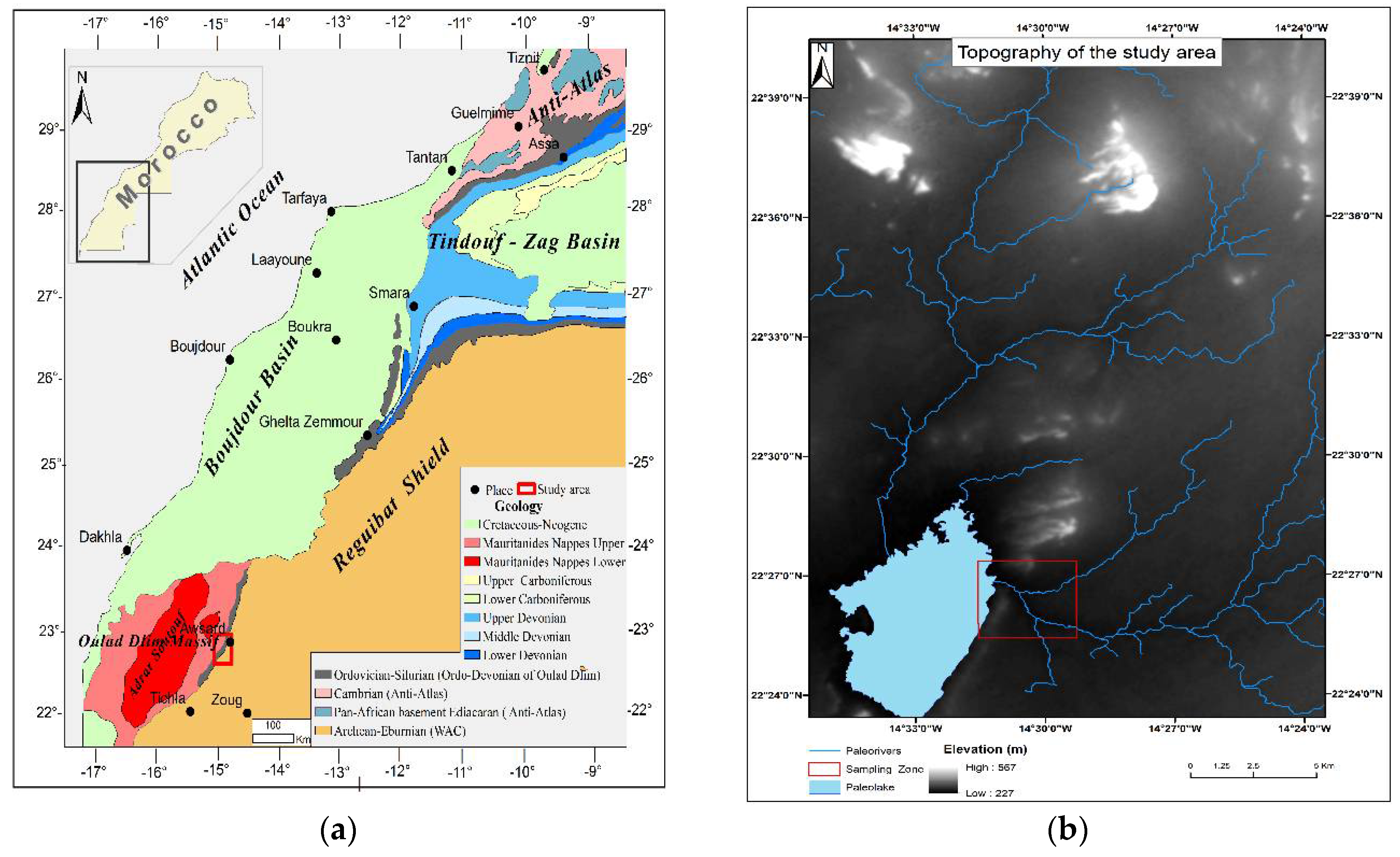
The study area is located in the southern Moroccan Sahara near the Morocco-Mauritanian border in the province of Awsard. This zone of 1000 km2 is delimited by the 14°20′ W and 14°36′ W meridians and by the 22°21′ N and 22°40′ N parallels. The study area has a Saharan desert climate typically dominated by low relief landscapes which are part of the Reguibat uplift, an important geological domain of the West African Craton (Figure 1a). The geological formations are mainly made of crystalline bedrock that consists of various igneous and metamorphic rocks dominated by granites, schist, gneisses and migmatites. These bedrock terrains are very tectonised and almost completely flattened, and covered by Paleozoic formations made mainly of schist, sandstones and quartzite (Figure 1b). The bedrock terrains and its Paleozoic cover deepen westwards under the Meso-Cenozoic formations of the Laayoune-Dakhla-Trafaya basin. Small layers of Quaternary deposits consist of detrital sediments of various types that are often less consolidated: fluvial, river-lake, slope and wind types also exist in the study area. The landscape is characterized by the presence of peneplains which alternate with prominent reliefs made of cuesta, outliers and scattered hills corresponding to inselberg, locally known as glebs. Most common quaternary deposits are the plains and river terraces, alluvial fans, glacis and peneplain with a thin mantle of sand and regs. The shapes of the most common quaternary deposits are the plains and river terraces, cones of dejection, glacis and peneplains. Those deposits with thin mantles of sand and regs carry thousands of tumuli and other evidence of prehistoric human occupation such as rock engravings.
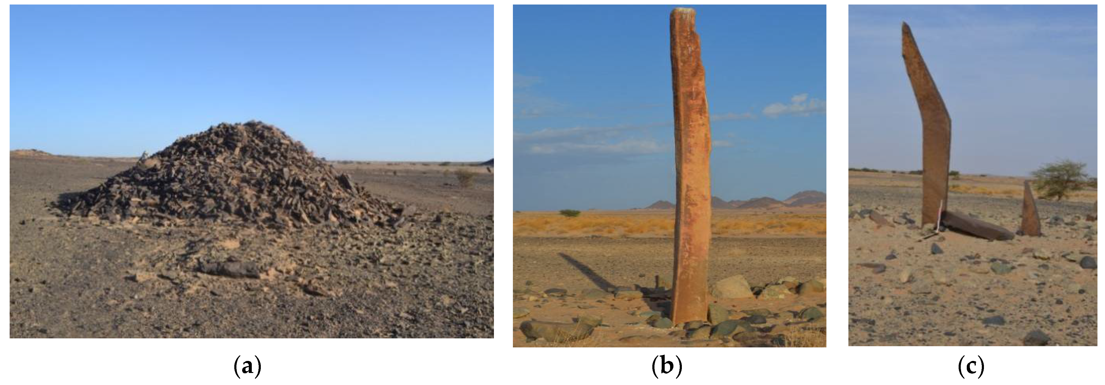
These tumuli of different types and diverse locations punctuate the landscape of the region around Awsard and clearly reflect those well known in other Moroccan regions [43]. Saharan tumuli are commonly of circular and conical shapes. They measure from 3 to 15 m in diameter and about 1 to 5 m in height (Figure 2a). Other kinds of crescent-moon shaped tumuli are also frequent, with a width of 2 to 6 m and 5 to 15 m length, their height vary from 1 to 5 m and they commonly possess two or rarely three antennas that can reach several tens of meters.
Rare funerary monuments called bazinat are spectacular in shape with 2 or 3 levels and sometimes they have an imposing size of 10 m diameter even more. The last type of Saharan Moroccan tumuli is the “Tumuli with long stone” whose length can reach 5 m (Figure 2b,c).
In order for predictive modelling of archaeological sites to succeed, quantifiable data are needed to create statistical statements about patterns on the locations of the sites [44]. On the other hand, spatial analysis of many environmental and archaeological variables in a GIS environment are required. Satellite imagery processing with a multi-criteria decision making approach based on the analysis of geological, geomorphological, archaeological profiles and GIS spatial analysis including slope, aspect, elevation and hydrologic-surface analysis were carried out. To obtain a wide spectrum of geo-environmental data for analysis, our work was based on topographical analysis of digital elevation models (DEM).
2.2. Data
2.2.1. Geo-Archaeological Database
This survey was conducted in six different field campaigns from 2014 up to 2017. The first field survey was carried between December 2014 and April 2017. Six field surveys were conducted in the Awsard area. The surveys were based on walking on the field with the aim of mapping all visible sites in the area. We worked with small mobile teams of three people equipped with a handheld GPS device, a tape measure and a compass. The task involved taking GPS coordinates, and the size and orientation of tumuli. Ultimately, we were able to cover 100% the area of our zone of interest (around 1000 km2). In total, the teams recorded 815 structures. The first mission focused on an area zone of 21 km2 where 233 sites were recorded. The data from this area that we called the “sampling zone” were used to develop the predictive model. After model development, we carried out five field surveys in the whole area, not only in high potential zones but also in low potential zones. A detailed geo-archaeological database was built in the ArcGIS (Esri, Redlands, CA, USA) environment with many attributes (name of site, geographic coordinate, type of site, geometric size of site, and type of rocks present in the sites, etc.) During the survey, we faced several challenges namely the fact that some tumuli were completely ransacked to the point that it was almost impossible to differentiate them from the background as we were in a rocky desert area. In addition, the sand depositions seemed to cover and hide some sites and visibility became extremely difficult in afternoon when the sun was strong.
2.2.2. Digital Elevation Model
- A SRTM DEM 1° arc-second image with a 30 m spatial resolution was downloaded from the United States Geological Survey (USGS) website http://earthexplorer.usgs.gov/
- An ASTER GDEM V2 images was downloaded from ASTER (Advanced Space-borne Thermal Emission and Reflection Radiometer) global DEM website http://www.jspacesystems.or.jp/ersdac/GDEM/E/4.html
- A DEM of the study area with 10 m cell size was generated through the digitization of contours and elevation points of a 1:50,000 scale topographic map.
2.2.3. Landsat ETM+ Multi-Spectral Image
A Landsat 7 ETM+ multi-spectral image, with 30 m spatial resolution of the study area, was obtained freely from the National Aeronautics and Space Administration (NASA) database http://earthexplorer.usgs.gov/, with many processing parameters including the supervised classification and band ratio technique.
2.3. Methodology
In this study, the methodology, which integrates GIS and multi-criteria evaluation, was used and applied to the Awsard area (Figure 3). The data analyses and processing in this study were based on both archaeological and geo-environmental information collected on 233 sites successively identified during first field survey campaign carried out on the sampling zone. At the end of the model set up, we realized a second field survey to collect data used to validate the models.
2.3.1. DEM Quality Assessment
However, before proceeding with the geo-environmental parameters analysis of Awsard, the reliability and accuracy of the DEM created by digitalization of contour lines from the topographic map was evaluated and compared to the Shuttle Radar Topography Mission (SRTM) DEM. The 30 m resolution DEMs were provided by ASTER. We used the equation of Schumann [45] to check the validity of different DEMs by comparing a number of reference points (datum points) (Table 1). The DEMs were validated by reference elevation data distributed across the study area. The height precision or quality of each DEM is expressed by Equation (1).
where RMSE is Root mean-square error, ER is the elevation of reference, EDEM is the elevation as provided by the different DEM data and n is the total number of points used as reference.
The RMSE for the DEM created through the digitized contour lines of the topographic maps was the lowest at 10.936 m, followed by the RMSE of the ASTER GDEM (global digital elevation model) with 12.26 m and the RMSE of SRTM DEM was the highest with 14.29 m. Moreover, from the results above, the DEM, which was produced by digitization of the topographic maps, became the basic layer of the terrain for further processing.
2.3.2. Geo-Archaeological Variables
As noted by Clement et al. [46], “The premise behind modelling of archaeological sites is that historic and prehistoric peoples were closely tied to their natural and cultural environment, and that these environments were a significant determinant in their choice of site location.” Predictive modelling examines soils (geology), distance to water sources, aspect, altitude and slope as potential environmental parameters or variables. GIS tools could be necessary for mapping and additional analysis such as buffer zoning, neighbouring computation and overlay analysis were used to construct a predictive model. The specific predictive model was built based on the use of a multi-parametric spatial analysis method of geographic elements, statistical and archaeological information in order to construct partial maps of archaeological interest [45,47,48]. The environmental factors, namely elevation, aspect, slope, distance from water sources, geology or rock types, were noted to have an influence on the choice of habitation in the Neolithic period in Awsard. These factors were statistically examined and assigned weight constraints according to expert knowledge. The cultural variables such as distance to the main settlement and/or ancient road proximity were used based on their availability for better accuracy of the model. However, as highlighted by Verhagen et al. [33] “cultural variables are rarely included in the models, thus resulting in predictions based on physical properties of the current landscape”. This may be explained by the fact that social and cognitive factors seem to be difficult to model as they are regarded as being too abstract and intangible for use in a predictive mode. Nevertheless, there is a lack of cultural data in the study area and archaeological researchers in the Saharan areas are only limited to rock arts and tumuli recording, notwithstanding settlements [49].
At the first stage of this analysis, we evaluated the functional relations between the locations of the archaeological sites and the following environmental parameters: elevation, slope, aspect, distance from water streams, and geology. Since the model variables change from one location to another, there are no fixed ranges and corresponding coefficients. Only statistical analysis of data collected in sampling zone allows coefficient assignment. Therefore, inside every variable, based on statistical analysis and number of expected and observed sites in an area, many classes were created with a corresponding coefficient consideration. The coefficient assignment is ruled by the following formula in Equation (2):
where Coef is the coefficient, Obs are the observed sites and Exp are the expected sites.
The theory behind this formula is to compare homogenous distribution of sites (expected according to percentage of the areas) against the observed distribution of sites. If observed sites are more than expected sites, the coefficient will be higher than 5, otherwise the coefficient will be less than 5.
Slope
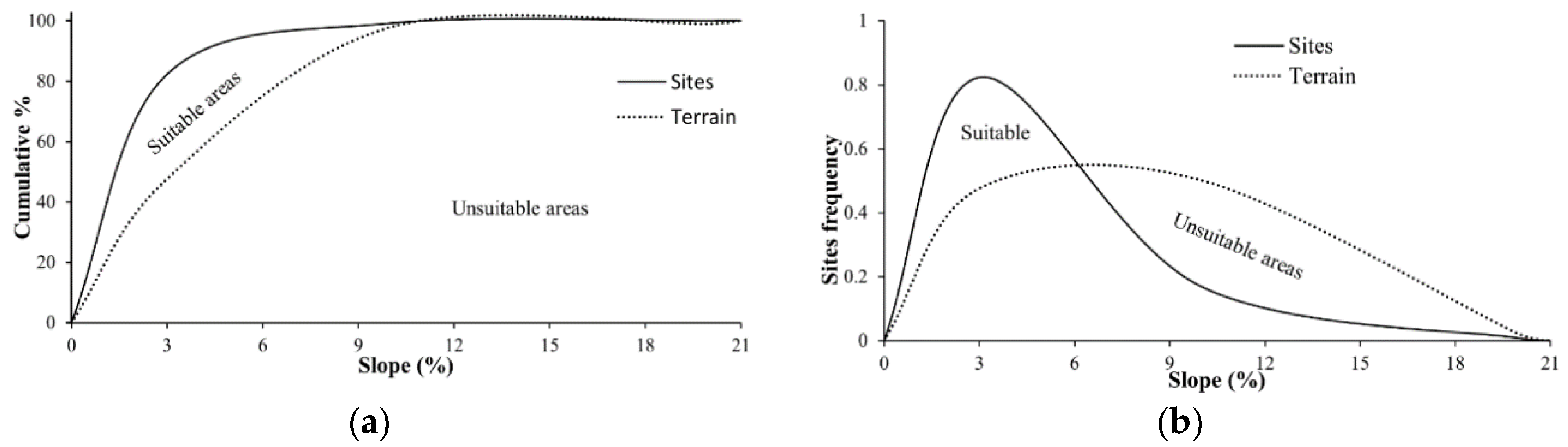
Slope is a direct function of the topography of a region [50]. Land slope is basic parameter for the construction of a predictive model. The basic argument here is that it is difficult to maintain a funeral mound on ground that is too steep since the steepness will increase the erodibility of the mound. Tumuli erection becomes impossible as a slope reaches certain values [7,51]. A layer consisting of slope (degree) data was generated by using the elevation grid as an input layer. The appropriate slope for tumuli is about 3–10%, the areas of this slope range were assigned a coefficient of 8. Therefore, steep areas with a slope of >20% were assigned a coefficient of 1, and gentle slope areas (0–3%) with a coefficient of 4 (Table 2). Slope seems to be a variable with little real predictive power, while almost 98% of all sites within the training area are located on terrain where the slope is between 0 and 10%, over 99% of the training area showed a slope of between 0% and 10% (Figure 3a,b). The vast majority of sites (47.64%) were found to be laid on plain areas (0–3% slope) and 50% of sites on 3–10% of terrain, thus it seems like Neolithic people occupied areas frequently located on landforms displaying low and moderate slopes.
Geology and Lithology
Geological formations and sediments bearing raw materials were identified using existing geological maps (Figure 1) improved by thematic maps generated from Landsat ETM+ images. Landsat 7 ETM+ band 1, band 3 and band 5 were used to produce a colour composite by applying the image-processing procedure known as “bands ratio”. Crósta and Moore [52] showed that this band combination is the most effective to discriminate rock types in semi-arid regions. The combination of spectral and texture characteristics mixed with supervised classification using previous field investigations (training sites) were used to identify and map rock types in the Awsard area. Five geological units including quartzite, schist, granites, sandstones, and sandy plain were identified. The accuracy assessment of the classified image was done through a matrix confusion approach [53,54]. Thereby overall accuracy found was 89%.
During the field survey, it turned out that the spatial distribution of archaeological sites is linked to the geomorphological setting and petrographic nature of the rocks. Thus, several types of geomorphological substrates of tumuli were distinguished. The most important are:
- the alluvial cones
- the pediments;
- the plains and river terraces;
- the cuesta cuff trays;
- the benches of the slopes of the valleys and below;
- the dykes through the vast flat surface;
- the precambrian plan crystalline basement.
Petrographic types of mound materials vary from one place to another and heavily depend on the lithology of the geological substrates and their neighbourhoods. When substrate belongs to the Precambrian, the most used stones are magmatic rocks (granitites, dolerites, gabbros and syenites) and other associated metamorphic rocks (serito-schist, light-grey quartzite, gneiss, migmatites, etc.); by contrast, when it consists of Paleozoic cover, the most used stones are quartzite and sandstones which are cut into slabs or plates that were used as steles in many tumuli. The availability of basic raw materials for use in erection of tumuli could be important [26]. The consolidated, hard and resistant materials are required for the construction of tumuli [55], which is why the areas with hard and resistant geological units including quartzite, schist and granite receive high coefficients, respectively 7, 6 and 5, while areas with soft and less resistant geological units receive low coefficient (1 for sandy plain and 4 for sandstones (Table 2)).
Aspect
There is a little pattern in the sites’ data to suggest that western aspect areas were less preferred than other aspects or exposures. A coefficient of 4 was affected to western exposure areas while northern aspect exposure areas received a coefficient of 6, and eastern and southern aspect exposure areas obtained a coefficient of 5 (Table 2).
Topography (Altitude)
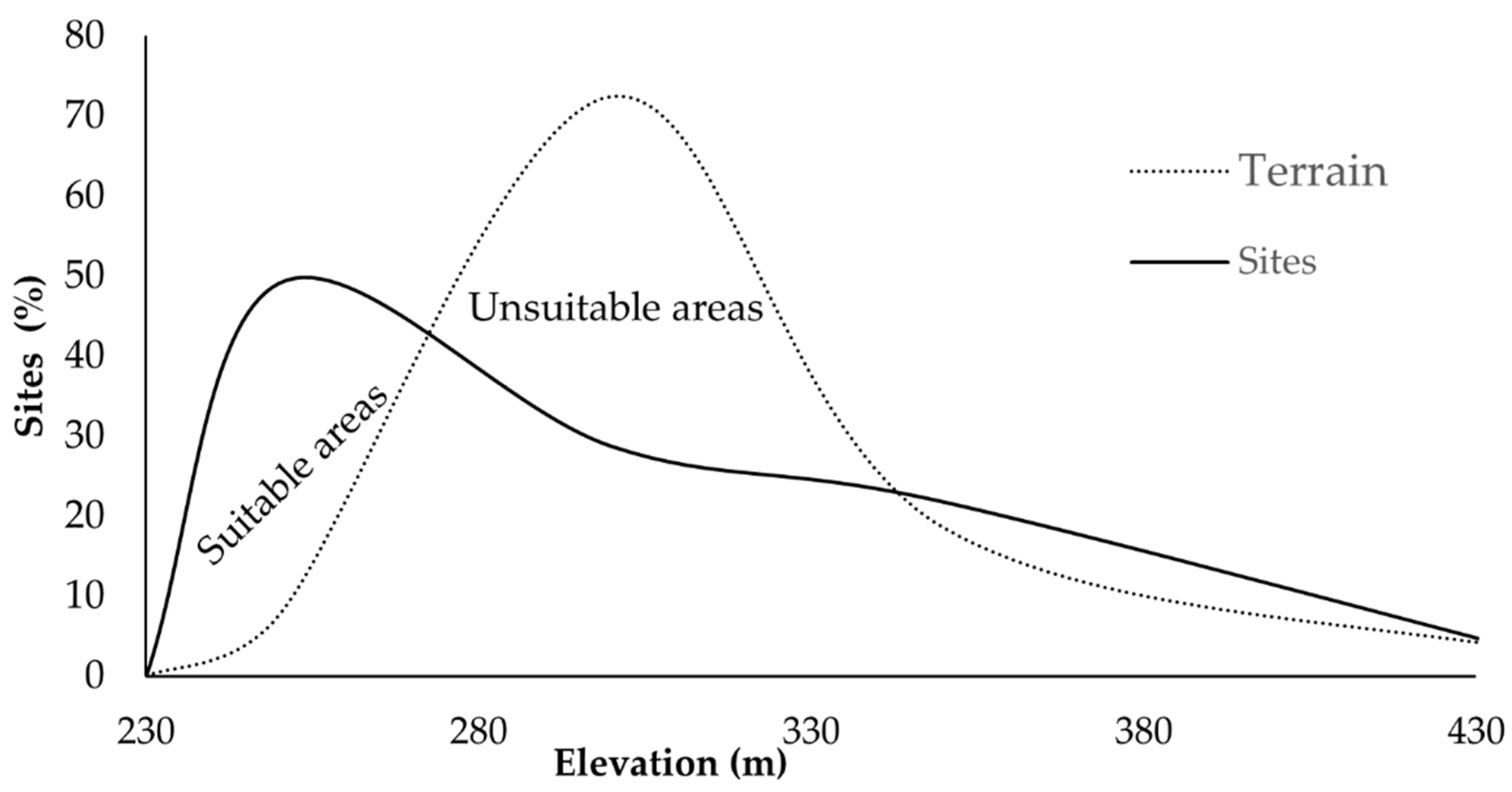
A greater concentration of archaeological sites has been recorded at lower altitudes in the study area (Figure 4). The spatial distribution of known sites in the model development zone known as the sampling zone permitted the range of 250–300 m to be defined as the most suitable altitude for site occurrence. Consequently, a coefficient of 6 was assigned to areas between 250 and 300 m (Table 2).
Distance to Water Source
Fresh water has always been a main factor for human occupation of any territory through history. The prehistoric population was set to occupy the areas within moderate distance close from the closest water sources [56]. In the study area and particularly in training site, 75% of sites are located in the areas less than 500 m from streams or lakes, and 98% of sites are located within 1 km distance close to water points. A coefficient of 7 has been given to areas within 100 and 250 m of a watershed, and a low coefficient of 1 to areas beyond 1 km from a watershed (Table 2).
2.3.3. Dependency between Variables and Sites
The geo-archaeological variables at the location of known sites are tested against the background environment as a whole to identify whether there are statistically significant differences between the distributions of sites against a particular geo-environmental variable [57]. Layers of geo-archaeological data are stored in 10 × 10 m raster grids in the GIS. Each grid cell receives a value for each geo-archaeological variable. The values for each of the geo-archaeological variables are also recorded for known archaeological site locations.
The values of these variables at known sites locations and their values across the entire study area are compared through the use of the Kolmogorov–Smirnov goodness-of-fit test [57]. This test examines the goodness-of-fit of a single sample to a referent population, and is appropriate for continuously distributed data, such as geo-environmental data [57]. The test is performed by plotting the cumulative distributions of the sample and population, respectively, and obtaining the difference (D) between these two curves. For a level of significance alpha = 0.05, for example, and in a two-tailed test, the value of d can be calculated from Equation (3):
In this research, 233 archaeological sites have been recorded in the study area, so n = 233 > 50; the formula above could be applied for determination of d which is equal to 0.089.
Here two hypotheses have been proposed:
- Null hypothesis (H0): that the sites are distributed irrespective of a given geo-environmental variable.
- Alternative hypothesis (H1): that the sites are distributed respective of a given geo-environmental variable.
If Dmax exceeds a critical value d (0.089), then H0 may be rejected and the sample distribution can be said to be different from the population distribution [34]. The Dmax for every geo-archaeological variable exceeds the critical value of 0.089, thus hypothesis H0 is rejected and consequently the sites are located with respect to slope, aspect, elevation, distance to watershed and geological units (Table 2).
The statistical analysis has been used in the coefficient assignment of each class of every model variable. As mentioned above, a zone of 21 km2 has been selected as the sampling zone in the predictive model’s development. All sites within this zone were recorded during the field survey. This zone contains 233 sites, and their spatial distribution with respect to environmental variables was statistically analysed and it has been proven that their distribution is governed by particular rules. Therefore, they are not randomly distributed, after all no population can colonize a given territory in a hazardous way. There are always determining factors. The coefficient given to each class indicates the level of potential to carry the sites of that given class. The higher value means many sites have been found within it.
2.3.4. Calculation of Class Coefficient and Weighting Variables
The method used to generate the archaeological predictive model (APM) is a multi-criteria evaluation (MCE), also known as multi-criteria decision analysis (MCDA). This method is based on various criteria combinations. Those criteria mainly correspond to the environmental variables that govern the suitability and unsuitability of a given area to host archaeological sites. The known sites’ location is not required as an input in this methodology but it has been used to strengthen the expert opinion of the Institut National de Science de l’Archéologie assigning weights to each variable before running the final model. MCE can be Boolean or categorical, weighted or unweighted. ArcGIS 10.2 (Esri), the program used to generate the APM, allows the choice of one of two methods: Boolean aggregation or weighted linear combination.
The Boolean aggregation method involves a binary division of each variable layer into suitable and unsuitable areas. These variables are then combined either inclusively (logical AND) or exclusively (logical OR). In the inclusive result, only the areas that are suitable in every layer become suitable in the final image. This is a risk-adverse strategy that ensures all qualities are high. In the exclusive result, an area that is suitable in only one layer will be suitable in the final result. This is a risk-taking strategy that ensures that only one quality is high. The weighted linear combination method is performed in two main steps. Firstly, each variable is classified on a continuous or categorical scale. A weight is then assigned to each individual variable with respect to how important it is compared to each of the other variables. Personal knowledge or expert opinion combined with statistical analysis of known sites’ locations are used to assign the weights. The final aggregation of data allows a trade-off between qualities, if necessary, so the final suitable area is not necessarily highly ranked with respect to every variable [58].
2.3.5. Principal Component Analysis
Principal components analysis (PCA) has been used in predictive models to eliminate multi-collinearity among variables. Multi-collinearity arises where there are very strong correlations among independent variables and consequently the independent variables have no significant impact on the dependent variable [59]. According to the Esri ArcGIS Resources Center website [60], the purpose of this spatial statistical technique (PCA) tool found in the Spatial Analyst toolbox of ArcGIS 10.2 is to eliminate multi-collinearity; for example, since elevation, slope, and aspect are derived from a DEM, from which most of the variance can be explained. The tool then creates a multiband raster that contains the same amount of bands as the specified number of components. The first principal component raster band contains the greatest amount of variance, the second contains the second greatest variance, and so on [60]. The first principal component rasters containing 95% of the variance were utilized in building the model.
2.3.6. Analytic Hierarchy Process
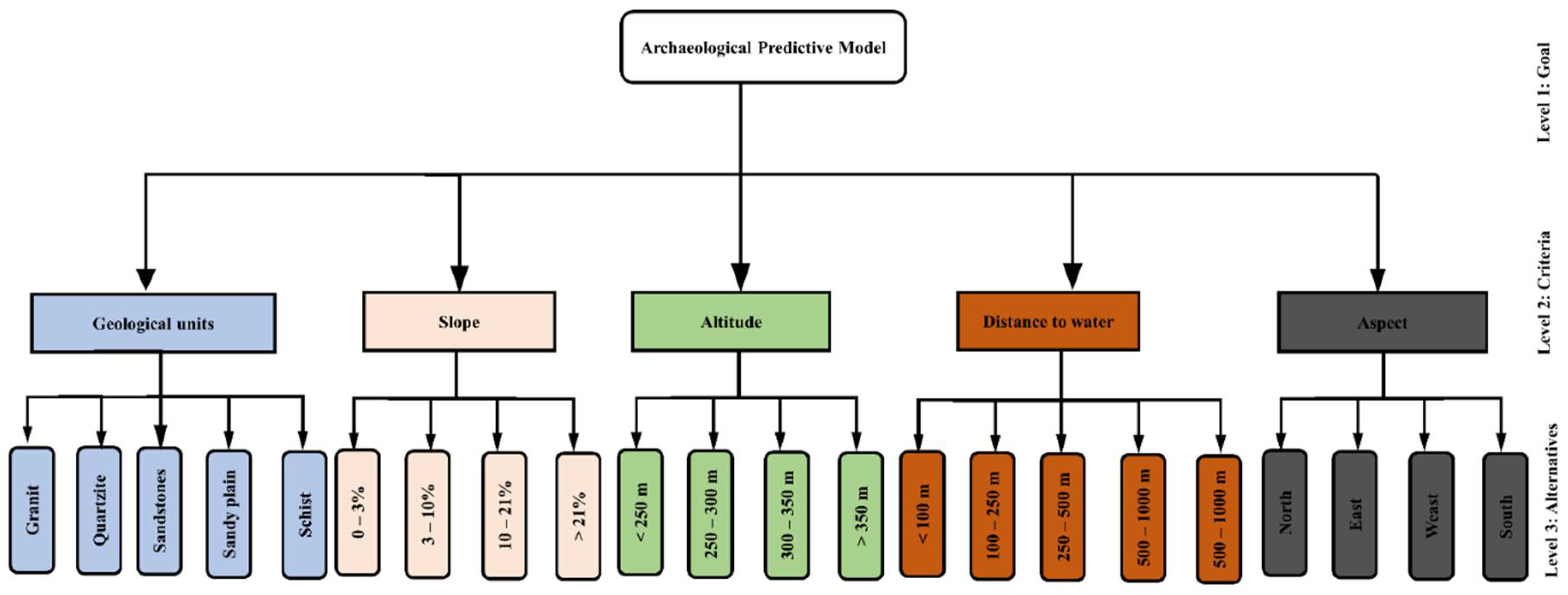
The AHP technique has used MCE approach in predictive modeling to locate archaeological sites. The AHP combines the criteria weights and the class scores, consequently determining a global score for each class, and a consequent ranking. The global score for a given class is a weighted sum of the scores it obtained with respect to all the criteria. Table 3 shows the method to assign weight to each parameter and classes in that parameter according to their importance. Value 9 shows high importance while value 1/9 shows low importance.
The AHP technique is based on different levels of analysis: level 1 is the goal of the analysis, level 2 is multi-criteria that consist of several factors influencing archaeological sites location in our case. Several other levels of sub criteria and sub-sub criteria can be added but in this current study only one level of sub-criteria has been used. The last level is the alternative choices (Figure 5). The lines between levels indicates the relationship between factors, choices and goal. In level 2, only one comparison matrix corresponds to pair-wise comparisons between 5 factors with respect to the goal (archaeological predictive model). Thus, the comparison matrix of level 2 has the size of 5 by 5, because each choice is connected to each factor.
A ratio matrix has been formed by the pairwise matrix comparison method. Criteria and sub-criteria in each level are in pairs with their importance to an element (criteria and sub-criteria) in the next higher level. Elements go to a downward level from a higher level [62]. The pairwise matrix can be expressed mathematically as follows:
The matrix has a reciprocal property which is expressed mathematically as:
After forming pairwise matrices as detailed in Table 4, weight vectors were calculated according to Satty’s eigenvector method. Weighting process consist of following two stages. First, the pairwise comparison matrix is normalized by Equation (6) and then the weights are computed by Equation (6) resulting in values in the table below (Table 5).
For all j = 1, 2, …, n
For all i = 1, 2, …, n.
The consistence index is determined using the the formula bellow:
whereas λmax is the highest or principal eigenvalue of the matrix.
In this study, λmax is equivalent to 5.324 according to computations, and n is the order of the matrix which is equal to 5, consequently CI calculated using Equation (8) is 0.081. The consistency ratio (CR) is an indicator of the degree of consistence in the pair-wise comparisons matrix. It is used as an indicator of establishment [63]. It can be calculated using the the formula of Equation (9):
where RI is the random consistency index which is equal to 1.12 as n = 5 according to Saaty [61].
A value of 0.072 has been obtained as the consistency ratio. Since this value of 0.072 for the proportion of inconsistency CR is less than 0.10, the judgments matrix is reasonably consistent and, therefore, can be used in the process of decision-making using AHP [64]. Otherwise, if CR ≥ 0.10 it means that pairwise consistency is inadequate, thus the original weights in the pairwise comparison matrix must be redone. After obtaining the weight of every criterion and its respective classes, the predictive model was produced in GIS using spatial overlay tools.
3. Results and Discussion
This predictive model for archaeological sites had interesting results. It showed that the areas with high potential of hosting archaeological sites are located in the southern zones of the study area. Other areas with a high probability of having archaeological sites are located near small isolated mountains that occupy the central part of the study area from north-east to south-west (Figure 6). The model provides a perspective on past occupation in the south of Morocco. Any populations always occupied the zones with favorable environments. The proximity to water sources played a major role in the determination of land suitability for Neolithic settlement and then in tumuli distrubution in the study area.
A sum of 365 out of 815 archaeological sites (45%) lay within 500 m distance of water sources, and 82% of sites are 1 km distance closer to paleorivers, while 284 sites (35%) are located around the paleolake in the south-western part of the study area, life always depends on water availability and accessibily since water reflects the image of society [65]. However, it must be mentioned that few sites are very close to water streams with only 14% of sites (115 tumuli) within a 100 m buffer zone of water bodies (Figure 6d). This can be explained by the fact that populations did not inhabit so close to rivers just to avoid flooding, because in the Neolithic period the Sahara was very humid with many river systems, lakes and marshes before it began to dry out during the long period of increasing aridity around 4000 BCE [66].
Lower slope terrains (Figure 6b) have as high a potential as archaeological sites as lower elevations (Figure 6c). This is normal since most people would not live on steepy and mountainious areas (Figure 7b). In general, flat areas tend to have the maximum of sites. Sites’ distribution also takes in consideration geological components (Figure 7a), after all certain materials are essential for tumuli construction. It turned out that 90% of sites (731 out of 815) were built on concrete rocks (granite, quartzite, schist and sandstones) against 10% of tumuli built on soft rocks especially in the sandy plain, but there are also some tumuli made of concrete raw materials from the neighbourhood (Figure 6a).
The predictive accuracy of any model must be verified to validate its efficacy. The formulation of the predictive model does not guarantee the accuracy of its predictions; our model was developed based on statistics of 233 known sites in the sampling zone (data collected during first field survey). After model realization, a second field campaign was carried out in order to test and validate the model efficiency, and for this focus more than 582 supplement sites were recorded; this means that a total of 815 sites were used in the development and validation of this predictive model.
Prediction accuracy assessment of this model expressed by gain estimation method according to Kvamme [67], is given by the Equation (10).
where PS is the total area where sites are predicted and OS are the observed sites within the area.
It has also been found that 56.87% of all sites are located in only 4.04% of the total area, and therefore this zone is qualified as a high potential zone for archaeological sites (Table 6). A gain of 92.87% was confirmed for this model, which is sufficient since archaeological prediction gains range from 1 (high predictive model) to 0 (no predictive model).
4. Conclusions
This study used a global methodology to create a predictive model that indicates areas with archaeological potentiality. The methodology involves archaeological research and geospatial techniques combined with multi-criteria decision making using AHP. The derivered predictive model (Figure 8) seems to be the best alternative and a useful tool for achaeological investigations for local archaeologists who usually have to monitorilarge areas with limited resources. The GIS has a huge range of applications for archaeology from recording a simple archaeological site, to managing thousands of sites and creating predictive models, etc. In this study the predictive model was used to predict archaeological sites’ locations, on the basis of observed patterns, on assumptions about human behavior. It was constructed through the application of GIS tool, remote-sensing data and archaeological field research data. The methodology has been applied successfully in the Moroccan Sahara to identify the locations of funeral monuments, where it provides accurate predictions.
The evaluation of the model demonstrated the validity of the proposed methodology. The prediction results, in the form of a prediction map with a gain of 92.8%, is sufficient to consider the model as reliable. When used as a contribution to archaeological field research, the aim is to identify small areas with high probability of hosting archaeological sites, and therefore further field investigations are required to confirm site presence. This study showed that a well-built predictive model can provide reliable predictions of where archaeological sites should and should not be located in a given landscape.
The use of GIS and remote sensing could considerably change the way archaeological survey and heritage management are done in Morocco. This paper showed how effective predictive modelling could enrich archaeological knowledge about ancient cultures. This paper highlighted the way geospatial technology applied in archaeological research could be an efficient solution to the limited funds involved in archaeology by minimizing and optimizing the area of interest for archaeological expeditions, since specific areas with a high probability of undiscovered archaeological remains are already known through the model.
This predictive model is recommended for Moroccan archaeologists to search other archaeological sites, and will make their work easier. Moreover, this tool can be used to promote geo-tourism by guiding tourists to areas with archaeological sites.
Author Contributions
Different authors has contributed to this article and their respective contribution is detailed as follow: Conceptualization, A.F.N. and H.R.; Methodology, A.F.N. and H.R.; Software, A.F.N. and H.R.; Validation, A.F.N. and H.R.; Formal Analysis, A.F.N. and H.R.; Investigation, A.F.N. and A.O.; Writing-Original Draft Preparation, A.F.N. and H.R.; Writing-Review & Editing, A.F.N., H.R. and K.M.; Visualization, A.F.N.; Supervision, H.R. and A.O.; Project Administration, A.O.; Funding Acquisition, A.O.
Funding
This research was partially funded by Awsard Province Administrative Council provided funding for this research, as part of its support of Ange Felix Nsanziyera PhD programme.
Acknowledgments
This study is a part of multidiscipline project named “Awsard Natural and Cultural Heritage Atlas” that aims to make a full inventory of all natural and archaeological heritage all-over the Saharan provinces of Morocco. The project was directed by the Moroccan Association of Rock Art (AMAR) and Association Nature-Initiative (ANI) in Collaboration with Directorate of Cultural Heritage of Morocco. Authors wish to thank all teams including diverse scientists, Association Nature Initiative of Dakhla (ANI), Awsard Province Administrative Council and other person who participated in the realization of this study.
Conflicts of Interest
The authors declare no conflict of interest. The founding sponsors had no role in the design of the study; in the collection, analyses, or interpretation of data; in the writing of the manuscript, and in the decision to publish the results.
References
- Souville, G. Les principaux types des tumuli marocains. Bulletin de la Société Préhistorique de France 1959, 56, 394–402. [Google Scholar] [CrossRef]
- Nami, M. L’épopée de la pierre à travers les temps préhistoriques, La pierre et son usage à travers les âges: Jardins des Hespérides. Bulletin Semestriel de La Société Marocaine d’Archéologie et du Patrimoine 2008, 4, 18–24. [Google Scholar]
- Nami, M.; Moser, J.; Mikdad, A.; Eiwanger, J. Quelques aspects de l’Iberomaurisien du Rif Oriental (Maroc). Bulletin d’Archéologie Marocaine 2012, 4, 16–33. [Google Scholar]
- Bokbot, Y. Neolothique et protohistoire du Maroc. In Proceedings of the Actes du IIIème Colloque International sur l’Histoire et l’Archéologie de l’Afrique du Nord, Tabarka, Tunisie, 8–13 May 2000; Edition de l’Institut National du Patrimoine: Tunis, Tunisia, 2000; pp. 35–45. [Google Scholar]
- Haidar-Boustani, M.; Iban, J.J.; Al-Maqdissi, M.; Armendari, A.; Gonzalez Urquijo, J.; Teira, L. Prospections Archaeologiques a l’ouest de la ville de homs: Rapport preliminaire campagne 2004. Annales D’Histoire et D’Archaeologie 2004, 16–17, 9–38. [Google Scholar]
- Rowlands, A.; Sarris, A. Detection of exposed and subsurface archaeological remains using multi-sensor remote sensing. J. Archaeol. Sci. 2007, 34, 795–803. [Google Scholar] [CrossRef]
- Siart, C.; Eitel, B.; Panagiotopoulos, D. Investigation of past archaeological landscapes using remote sensing. J. Archaeol. Sci. 2008, 35, 2918–2926. [Google Scholar] [CrossRef]
- Kamermans, H. Smashing the crystal ball. A critical evaluation of the Dutch national archaeological predictive model (IKAW). Int. J. Hum. Arts Comput. 2007, 1, 71–84. [Google Scholar] [CrossRef]
- McCauley, J.F.; Schaber, G.G.; Breed, C.S.; Grolier, M.J.; Haynes, C.V.; Issawi, B.; Elachi, C.; Blom, R. Subsurface valleys and geoarchaeology of the eastern Sahara revealed by shuttle radar. Science 1982, 281, 1004–1020. [Google Scholar] [CrossRef] [PubMed]
- Bewley, R.; Donoghue, D.; Gaffney, V.; Van Leusen, M.; Wise, A. Archiving Aerial Photography and Remote Sensing Data: A Guide to Good Practice; Archaeology Data Service; Oxbow Books: Oxford, UK, 1999. [Google Scholar]
- Wynn, J.C. Applications of high-resolution geophysical methods to archaeology. In Archaeological Geology of North America Centennial Special Volume; Lasca, N.P., Donahue, J., Eds.; Geological Society of America: Boulder, CO, USA, 1990; pp. 603–617. [Google Scholar]
- Theocaris, P.S.; Liritzis, I.; Lagios, E.; Sampson, A. Geophysical prospection, archaeological excavation, and dating in two Hellenic pyramids. Surv. Geophys. 1996, 17, 593–618. [Google Scholar] [CrossRef]
- Gaffney, C.; Gaffney, V. Non-invasive investigations at Wroxeter at the end of the twentieth century. J. Archaeol. Prospect. 2000, 7, 65–67. [Google Scholar] [CrossRef]
- Jones, R.E.; Sarris, A.J. Geophysical and related techniques applied to archaeological survey in the Mediterranean: A review. J. Mediterr. Archaeol. 2000, 13, 3–75. [Google Scholar]
- Neubauer, W. Images of the invisible-prospection methods for the documentation of threatened archaeological sites. Naturwissenschaften 2001, 88, 13–24. [Google Scholar] [CrossRef] [PubMed]
- Kvamme, K.L. Geophysical surveys as landscape archaeology. Am. Antiq. 2003, 68, 435–457. [Google Scholar] [CrossRef]
- Montufo, A.M. The use of satellite imagery and digital image processing in landscape archaeology: A case study from the island of Mallorca, Spain. Geoarchaeology 1997, 2, 71–85. [Google Scholar] [CrossRef]
- Powlesland, D.; Lyall, J.; Donoghue, D. Enhancing the record through remote sensing: The application and integration of multi-sensor, non-invasive remote sensing techniques for the enhancement of the Sites and Monuments Record. Heslerton Parish Project, N. Yorkshire, England. Internet Archaeol. 1997, 2. [Google Scholar] [CrossRef]
- Fowler, M.J.F. Satellite remote sensing and archaeology: A comparative study of satellite imagery of the environs of Figsbury Ring, Wiltshire. J. Archaeol. Prospect. 2002, 9, 55–69. [Google Scholar] [CrossRef]
- Banes, I. Aerial remote-sensing techniques used in the management of archaeological monuments on the British Army’s Salisbury Plain Training Area Wiltshire, UK. J. Archaeol. Prospect. 2003, 10, 83–90. [Google Scholar] [CrossRef]
- Devereux, B.J.; Amable, G.S.; Crow, P.; Cliff, A.D. The potential of airborne lidar for detection of archaeological features under woodland canopies. Antiquity 2005, 79, 648–660. [Google Scholar] [CrossRef]
- Challis, K. Airborne laser altimetry in alluviated landscapes. J. Archaeol. Prospect. 2006, 13, 103–127. [Google Scholar] [CrossRef]
- Lasaponara, R.; Masini, N. Satellite Remote Sensing: A New Tool for Archaeology; Springer Science & Business Media: Cham, The Netherlands, 2012. [Google Scholar]
- Chen, R.; Lasaponar, R.; Masini, N. An overview of satellite synthetic aperture radar remote sensing in archaeology: From site detection to monitoring. J. Cult. Herit. 2015, 23, 5–11. [Google Scholar] [CrossRef]
- Tapete, D.; Cigna, F. Trends and perspectives of space-borne SAR remote sensing for archaeological landscape and cultural heritage applications. J. Archaeol. Sci. Rep. 2017, 14, 716–726. [Google Scholar] [CrossRef] [Green Version]
- Van der Meer, F.D.; De Jong, S.M. Introduction. In Imaging Spectrometry: Basic Principles and Prospective Applications; Van der Meer, F.D., de Jong, S.M., Eds.; Kluwer Academic Publishers: Dordrecht, The Netherlands, 2001; pp. XXI–XXIII. [Google Scholar]
- Kumar, L.; Schmidt, K.; Dury, S.; Skidmore, A. Imaging spectrometry and vegetation science. In Imaging Spectrometry: Basic Principles and Prospective Applications; Van der Meer, F.D., de Jong, S.M., Eds.; Kluwer Academic Publishers: Dordrecht, The Netherlands, 2001; pp. 111–155. [Google Scholar]
- Lucas, R.M.; Rowlands, A.P.; Niemann, O.; Merton, R. Hyperspectral sensors: Past, present and future. In Advanced Image Processing Techniques for Remotely Sensed Hyperspectral Data; Varshney, P.K., Arora, M.K., Eds.; Springer: Berlin/Heidelberg, Germany, 2004; pp. 11–40. [Google Scholar]
- Huggett, J. Looking at intra-site GIS. In CAA96 Computer Applications and Quantitative Methods in Archaeology; Lockyear, K., Sly, T.J.T., Mihailescu-Birliba, V., Eds.; BAR International Series 845; Archaeopress: Oxford, UK, 2000; pp. 117–122. [Google Scholar]
- Vullo, N.; Fontana, F.; Guerreschi, A. The application of GIS to intra-site spatial analysis: Preliminary results from Alpe Veglia (VB) and Mondeval de Sora (BL), two Mesolithic sites in the Italian Alps. In New Techniques for Old Times: CAA98; Barcelo, J.A., Briz, I., Vila, A., Eds.; British Archaeological Reports International Series 757; Archaeopress: Oxford, UK, 1999; pp. 111–116. [Google Scholar]
- Robinson, J.; Zubrow, E. Between space space: Interpolation in Archaeology. In Geographical Information Systems and Landscaoe Archaeology; Gillings, M., Mattingly, D., Dalem, J.V., Eds.; Oxbow Books: Oxford, UK, 1999; pp. 65–84. [Google Scholar]
- Wheatley, D.; Gillings, M. Spatial technology and archaeology. In The Archaeological Applications of GIS 2002; Taylor and Francis: London, UK, 2002. [Google Scholar] [CrossRef]
- Verhagen, P. Case studies in Archaeological Predictive Modelling; Archaeological Studies Leiden University; Leiden University Press: Leiden, The Netherlands, 2007. [Google Scholar]
- Wheatley, D. Cumulative viewshed analysis: A GIS-based method for investigating intervisibility, and its archaeological applications. In Archaeology and Geographical Information Systems: A European Perspective; Lock, G., Stančič, Z., Eds.; Taylor & Francis: London, UK, 1995; pp. 171–185. [Google Scholar]
- Wheatley, D. The use of GIS to understand regional variation in Neolithic Wessex. In New Methods, Old Problems: Geographic Information Systems in Modern Archaeological Research; Maschner, H.D.G., Ed.; Occasional Paper No. 23; Center for Archaeological Investigations, Southern Illinois University: Carbondale, IL, USA, 1996; pp. 75–103. [Google Scholar]
- Wheatley, D. Making space for an archaeology of place. Internet Archaeol. 2004, 15. [Google Scholar] [CrossRef]
- Roeloffs, A.; Wiatr, T.; Reicherter, K.; Museum, S.N. Prospection of Karstic Caves Using Gis and Remote Sensing. In Proceedings of the ISPRS WG VII/5 Workshop, Cologne, Germany, 18–19 November 2011; pp. 107–115. [Google Scholar]
- Belmonte, J.; Esteban, C.; Cuesta, L.; Perera Betancort, M.; Gonzarez, J. Pre-Islamic burial moniments in Northern and Saharn Morocco. Archaeoastronomy 1999, 30, 21. [Google Scholar] [CrossRef]
- Linstädter, J.; Blatt, M. Sea, slopes and shelters: Archaeological Surveys along the Mediterranean Coast, west of the Melilla Peninsula (Morocco). In Pleistocene Foragers: Their Culture and Environment; Pastoors, A., Aufferman, B., Eds.; Wissenschaftliche Schriften des Nneanderthal Museums: Mettmann, Germany, 2013; pp. 27–32. [Google Scholar]
- Di Lernia, S. Places, monuments, and landscape: Evidence from the Holocene central Sahara, Azania. Archaeol. Res. Afr. 2013, 48, 173–192. [Google Scholar] [CrossRef]
- Galan, E.; Torres, J.; Senoran, J.M. Archaeological Interventions. In Search of Traces of the Human Presence in the Valley. Complutum 2014, 25, 45–76. [Google Scholar]
- Pappu, S.; Akhilesh, K.; Ravindranath, S.; Raj, U. Applications of satellite remote sensing for research and heritage management in Indian prehistory. J. Archaeol. Sci. 2010, 37, 2316–2331. [Google Scholar] [CrossRef]
- Brooks, N.; Clarke, J.; Garfi, S.; Pirie, A. The archaeology of Western Sahara: Results of environmental and archaeological reconnaissance. Antiquity 2009, 83, 918–934. [Google Scholar] [CrossRef]
- Kohler, T.A. Predictive locational modelling: History and current practice. In Quantifying the Present and Predicting the Past: Theory, Method and Application of Archaeological Predictive Modeling; Judge, W.L., Sebastian, L., Eds.; US Bureau of Land Management: Denver, CO, USA, 1988; pp. 19–59. [Google Scholar]
- Alexakis, D.; Sarris, A.; Astaras, T.; Albanakis, K. Integrated GIS, remote sensing and geomorphologic approaches for the reconstruction of the landscape habitation of Thessaly during the neolithic period. J. Archaeol. Sci. 2011, 38, 89–100. [Google Scholar] [CrossRef]
- Clement, O.C.; Sahadeb, D.; Kloot, R. Using GIS to Predict Likely Archaeological Sites. Available online: https://digitalcommons.du.edu/cgi/viewcontent.cgi?article=1056&context=geog_ms_capstone (accessed on 22 June 2017).
- Makepeace, G.A. The Prehistoric Archaeology of Settlement in South-East Wales and the Borders; Archaeopress: Oxford, UK, 2006; pp. 25–26. [Google Scholar]
- Van Leusen, M.; Deeben, J.; Hallewa, D.; Zoetbrood, P.; Kamerman, H.; Verhagen, P. Predictive Modelling for Archaeological Heritage Management: A Research Agenda; van Leusen, P.M., Kamermans, H., Eds.; Rijksdienst voor het Oudheidkundig Bodemonderzoek: Amersfoort, The Netherlands, 2004. [Google Scholar]
- Di Lernia, S. The archaeology of rock art in Northern Africa. In The Oxford Handbook of the Archaeology and Anthropology of Rock Art; David, B., McNiven, I., Eds.; Oxford University Press: Oxford, UK, 2017. [Google Scholar] [CrossRef]
- Canning, S. “BELIEF” in the past: Dempster-Shafer theory, GIS and archaeological predictive modelling. Aust. Archaeol. 2005, 60, 6–15. [Google Scholar] [CrossRef]
- Mink, P.B.; Ripy, J.; Bailey, K. Predictive archaeological modeling using gis-based fuzzy set estimation: A case study in Woodford County, Kentucky. In Proceedings of the 88th Annual Meeting on Transportation Research Board, Washington DC, USA, 11–15 January 2009. [Google Scholar]
- Crósta, A.P.; Moore, J.M. Geological mapping using Landsat Thematic Mapper imagery in Almeria Province, south-east Spain. Int. J. Remote Sens. 1989, 10, 505–514. [Google Scholar] [CrossRef]
- Congalton, R.G. A review of assessing the accuracy of classifications of remotely sensed data. Remote Sens. Environ. 1991, 37, 35–46. [Google Scholar] [CrossRef]
- Foody, G.M. Status of land cover classification accuracy assessment. Remote Sens. Environ. 2002, 80, 185–201. [Google Scholar] [CrossRef]
- Diggs, D.M.; Brunswig, R.H. Weights of Evidence Modeling in Archaeology in Rocky Mountain National Park. In Proceedings of the ESRI International User Conference, San Diego, CA, USA, 12–16 July 2010; Available online: http://www.unco.edu/geography/faculty/diggs/docs/diggs_brunswig_esri_2009b_ppoint2003.ppt (accessed on 21 July 2014).
- Yang, L.; Pei, A.; Guo, N.; Liang, B. Spatial Modality of Prehistoric Settlement Sites in Luoyang Area. Sci. Geogr. Sin. 2012, 32, 993–999. [Google Scholar]
- Kvamme, K.L. One-Sample Tests in Regional Archaeological Analysis: New Possibilities through Computer Technology. Am. Ant. 1990, 55, 367–381. [Google Scholar] [CrossRef]
- Eastman, J.R. IDRISI Kilimanjaro Guide to GIS and Image Processing; Clark Univesity: Worcester, MA, USA, 2003. [Google Scholar]
- Fattah, M.A. Multicollinearity. Central Michigan University, 2010. Available online: http://www.chsbs.cmich.edu/fattah/courses/empirical/multicollinearity.html (accessed on 15 May 2014).
- Esri. How Principal Component Analysis Works. Retrieved from ArcGIS Resource Center. Available online: http://help.arcgis.com/en/arcgisdesktop/10.0/help/index.html#/How_Principal_Co mponents_works/009z000000qm000000/ (accessed on 7 May 2014).
- Saaty, T.L. The Analytical Hierarchy Process; McGraw Hill: New York, NY, USA, 1980. [Google Scholar]
- Malczewski, J. GIS and Multicriteria Decision Analysis; John Wiley & Sons, Inc.: Toronto, ON, Canada, 1999. [Google Scholar]
- Chandio, I.A. GIS-basedland suitability analysis of sustainable hillside development. In Proceedings of the Fourth International Symposium on Infrastructure Engineering in Developing Countries, Karachi, Pakistan, 11–13 December 2013. [Google Scholar] [CrossRef]
- Park, S.; Jeon, S.; Kim, S.; Choi, C. Prediction and Comparaison of Urban Growth by Land Suitability Index Mapping Using GIS and RS in South Korea. Landsc. Urban Plan. 2011, 99, 104–114. [Google Scholar] [CrossRef]
- Mithen, S. The domestication of water: Water management in the ancient world and its prehistoricorigins in the jordan valley. Philos. Trans. R. Soc. Lond. A Math. Phys. Eng. Sci. 2010, 368, 5249–5274. [Google Scholar] [CrossRef] [PubMed]
- Joanne, C.; Brooks, N.; Banning, E.B.; Matthewsd, M.; Campbell, S.; Clare, L.; Cremaschi, M.; di Lernia, S.; Drake, N.; Gallinaro, M.; et al. Climatic changes and social transformations in the Near East and North Africa during the ‘long’ 4th millennium BC: A comparative study of environmental and archaeological evidence. Quat. Sci. Rev. 2016, 136, 96–121. [Google Scholar] [CrossRef] [Green Version]
- Kvamme, K.L. Development and testing of Quantitative models. In Quantifying the Present and Predicting the Past: Theory, Method and Application of Archaeological Predictive Modelling; Judge, W., Sebastian, L., Eds.; Bureau of Land Management: Denver, CO, USA, 1988; pp. 325–428. [Google Scholar]
Figure 1.
Geological maps: (a) background after the geological map of Morocco, scale 1:1,000,000; (b) topography (digital elevation model, DEM) map of study area.
Figure 1.
Geological maps: (a) background after the geological map of Morocco, scale 1:1,000,000; (b) topography (digital elevation model, DEM) map of study area.

Figure 2.
Tumuli in the Awsard area: (a) conical tumulus, (b,c) long stone tumuli.

Figure 3.
Sites repartition in relation to slope: (a) cumulative repartition; (b) site frequency.

Figure 4.
Sites’ location in relation with elevation.

Figure 5.
Different level of analytic hierarchy process (AHP).

Figure 6.
Partial maps of different geo-environmental variables: (a) geology; (b) slope; (c) elevation; (d) distance to water sources.
Figure 6.
Partial maps of different geo-environmental variables: (a) geology; (b) slope; (c) elevation; (d) distance to water sources.
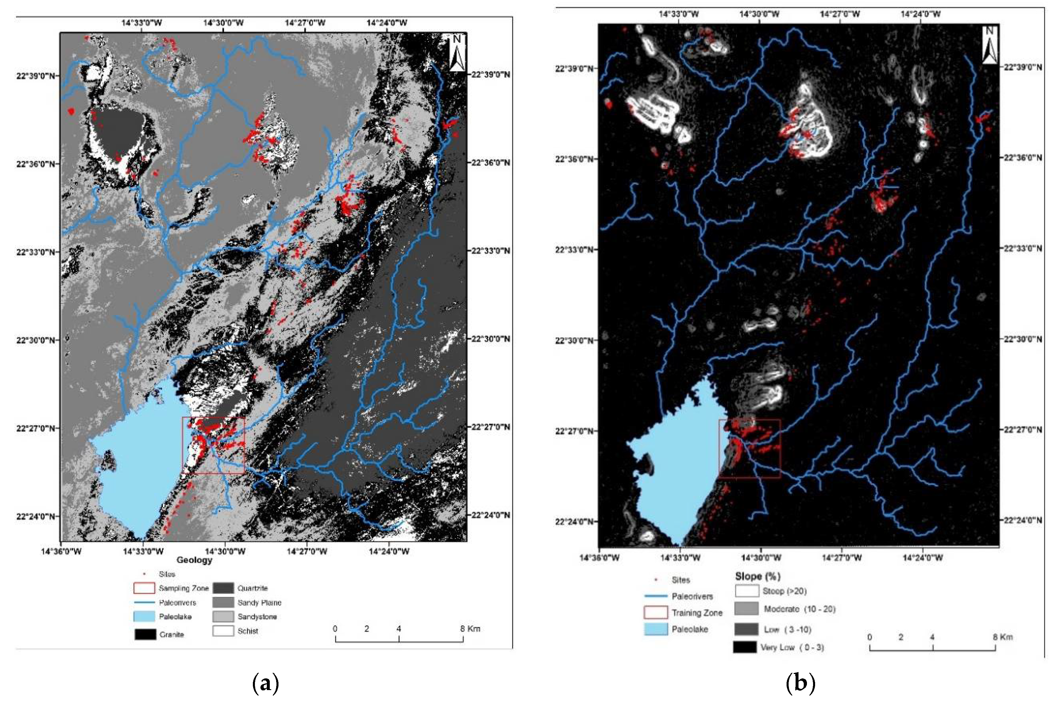

Figure 7.
Sites’ distribution in study area. (a) In respect to geological unit; (b) In respect to slope; (c) In respect to elevation; (d) In respect to distance to water sources.
Figure 7.
Sites’ distribution in study area. (a) In respect to geological unit; (b) In respect to slope; (c) In respect to elevation; (d) In respect to distance to water sources.
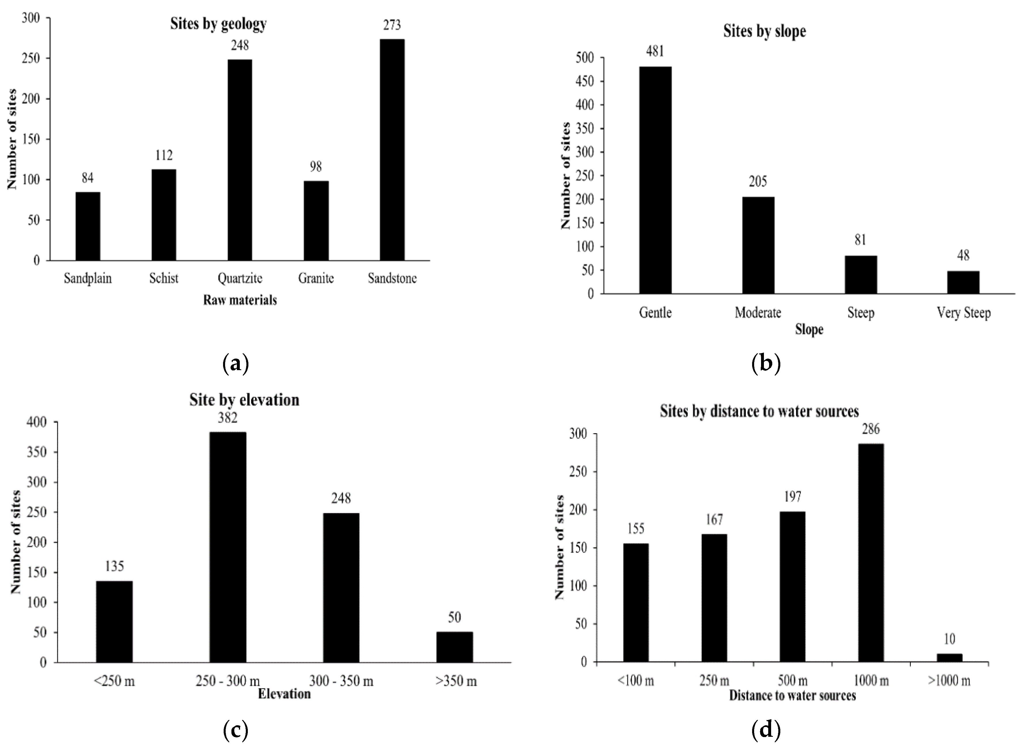
Figure 8.
Archaeological predictive map of sites in Awsard.


Table 1.
DEM quality assessment.
| ER (m) | EDEM TOPO (m) | EDEM ASTER (m) | EDEM SRTM (m) | (ER − EDEM TOPO)2 (m) | (ER − EDEMA STER)2 (m) | (ER − EDEM SRTM)2 (m) |
|---|---|---|---|---|---|---|
| 338 | 329 | 333 | 330 | 81 | 25 | 64 |
| 346 | 343 | 368 | 321 | 9 | 484 | 625 |
| 286 | 280 | 275 | 277 | 36 | 121 | 81 |
| 283 | 268 | 273 | 253 | 225 | 100 | 900 |
| 277 | 279 | 284 | 276 | 4 | 49 | 1 |
| 276 | 272 | 261 | 271 | 16 | 225 | 25 |
| 289 | 291 | 274 | 277 | 4 | 225 | 144 |
| 302 | 318 | 290 | 293 | 256 | 144 | 81 |
| 334 | 356 | 337 | 334 | 484 | 9 | 0 |
| 283 | 274 | 272 | 272 | 81 | 121 | 121 |
| 119.6 | 150.3 | 204.2 | ||||
| 10.936 | 12.260 | 14.290 |
Table 2.
Kolmogorov–Smirnov goodness-of-fit test for some variables.
| Class | Expectations (Sampling Zone) | Observations (Sampling Zone) | Coefficient | D | ||||||
|---|---|---|---|---|---|---|---|---|---|---|
| Area km2 | Area % | Expected | Cumulative Frequency | Sites | % Sites | Cumulative Frequency | ||||
| Slope in % | 0–3 | 17.40 | 82.29 | 192 | 0.823 | 111 | 47.64 | 0.476 | 4 | 0.347 |
| 3–10 | 3.57 | 16.91 | 39 | 0.992 | 119 | 51.07 | 0.987 | 8 | 0.005 | |
| 10–20 | 0.17 | 0.80 | 2 | 1 | 3 | 1.29 | 1.000 | 6 | 0.000 | |
| >20 | 0.00 | 0.00 | 0 | 1 | 0 | 0.00 | 1 | 1 | 0.000 | |
| n = | 21.14 | 100 | 233 | 233 | 100 | Dmax = | 0.347 | |||
| Geological unit | Quartzite | 1.42 | 10.23 | 24 | 0.102 | 48 | 20.60 | 0.206 | 7 | 0.104 |
| Schist | 2.19 | 15.83 | 37 | 0.261 | 54 | 23.18 | 0.438 | 6 | 0.177 | |
| Granite | 2.84 | 20.49 | 48 | 0.466 | 57 | 24.46 | 0.682 | 5 | 0.217 | |
| Sandstone | 6.68 | 48.27 | 112 | 0.948 | 74 | 31.76 | 1.000 | 4 | 0.052 | |
| Sandy Plain | 0.72 | 5.18 | 12 | 1 | 0 | 0.00 | 1 | 1 | 0.000 | |
| n = | 13.84 | 100 | 233 | 233 | 100 | Dmax = | 0.217 | |||
| Dist. water (m) | <100 | 4.32 | 26.50 | 62 | 0.265 | 40 | 17.17 | 0.172 | 4 | 0.093 |
| 100–250 | 3.62 | 22.20 | 52 | 0.487 | 66 | 28.33 | 0.455 | 6 | 0.032 | |
| 250–500 | 4.30 | 26.38 | 61 | 0.751 | 68 | 29.18 | 0.747 | 5 | 0.004 | |
| 500–1000 | 3.53 | 21.68 | 51 | 0.968 | 54 | 23.18 | 0.979 | 5 | 0.011 | |
| >1000 | 0.53 | 3.24 | 7.56 | 1 | 5 | 2.15 | 1 | 4 | 0.000 | |
| n = | 16.29 | 100 | 233 | 233 | 100 | Dmax = | 0.093 | |||
| Elevation (m) | <250 | 1.62 | 7.66 | 17.85 | 0.08 | 116 | 49.79 | 0.498 | 9 | 0.421 |
| 250–300 | 15.30 | 72.37 | 168.62 | 0.80 | 66 | 28.33 | 0.781 | 3 | 0.019 | |
| 300–350 | 3.90 | 18.45 | 42.99 | 0.98 | 51 | 21.89 | 1.000 | 5 | 0.015 | |
| >350 | 0.32 | 1.52 | 3.54 | 1.00 | 0 | 0.00 | 1.0 | 0 | 0.000 | |
| n = | 21.14 | 100 | 233 | 233 | 100 | Dmax = | 0.421 | |||
| Aspect | North | 4.09 | 19.35 | 45.08 | 0.19 | 55 | 23.61 | 0.24 | 5 | 0.043 |
| East | 4.53 | 21.42 | 49.91 | 0.41 | 61 | 26.18 | 0.50 | 5 | 0.090 | |
| South | 4.91 | 23.24 | 54.15 | 0.64 | 53 | 22.75 | 0.73 | 5 | 0.085 | |
| West | 7.61 | 35.99 | 83.86 | 1.00 | 64 | 27.47 | 1.00 | 4 | 0.000 | |
| n = | 21.14 | 100 | 233 | 233 | 100 | Dmax = | 0.090 | |||
Table 3.
Pair-wise comparison matrix formulation.
| 1/9 | 1/7 | 1/5 | 1/3 | 1 | 3 | 5 | 7 | 9 |
|---|---|---|---|---|---|---|---|---|
| Extremely | Very Strongly | Strongly | Moderately | Equally | Moderately | Strongly | Very Strongly | Extremely |
| Less important | Very important | |||||||
Source: Saaty [61]. Note: 1/8, 1/6, 1/4, 1/2, 2, 4, 6 and 8 can be used if more classes exist.
Table 4.
Pair-wise comparison matrix.
| Geology | Slope | Elevation | Distance Water | Aspect | |
|---|---|---|---|---|---|
| Geology | 1.000 | 1.500 | 2.000 | 6.000 | 6.000 |
| Slope | 0.667 | 1.000 | 1.330 | 4.000 | 4.000 |
| Elevation | 0.500 | 0.752 | 1.000 | 3.000 | 3.000 |
| Distance water | 0.167 | 0.250 | 0.333 | 1.000 | 1.000 |
| Aspect | 0.167 | 0.250 | 0.333 | 1.000 | 1.000 |
Table 5.
Normalized pair-wise comparison matrix.
| Geology | Slope | Elevation | Distance Water | Aspect | Priority | |
|---|---|---|---|---|---|---|
| Geology | 0.400 | 0.400 | 0.400 | 0.400 | 0.400 | 0.400 |
| Slope | 0.267 | 0.267 | 0.266 | 0.267 | 0.267 | 0.267 |
| Elevation | 0.200 | 0.200 | 0.200 | 0.200 | 0.200 | 0.200 |
| Distance water | 0.067 | 0.067 | 0.067 | 0.067 | 0.067 | 0.067 |
| Aspect | 0.067 | 0.067 | 0.067 | 0.067 | 0.067 | 0.067 |
Table 6.
Predictive gain computation.
| Prediction | Area (%) | Sites (Number) | Sites (%) |
|---|---|---|---|
| Low | 40.50 | 56 | 9.62 |
| Medium | 55.46 | 195 | 33.50 |
| High | 4.04 | 331 | 56.87 |
© 2018 by the authors. Licensee MDPI, Basel, Switzerland. This article is an open access article distributed under the terms and conditions of the Creative Commons Attribution (CC BY) license (http://creativecommons.org/licenses/by/4.0/).
Share and Cite
MDPI and ACS Style
Nsanziyera, A.F.; Rhinane, H.; Oujaa, A.; Mubea, K. GIS and Remote-Sensing Application in Archaeological Site Mapping in the Awsard Area (Morocco). Geosciences 2018, 8, 207. https://doi.org/10.3390/geosciences8060207
AMA Style
Nsanziyera AF, Rhinane H, Oujaa A, Mubea K. GIS and Remote-Sensing Application in Archaeological Site Mapping in the Awsard Area (Morocco). Geosciences. 2018; 8(6):207. https://doi.org/10.3390/geosciences8060207
Chicago/Turabian StyleNsanziyera, Ange Felix, Hassan Rhinane, Aicha Oujaa, and Kenneth Mubea. 2018. "GIS and Remote-Sensing Application in Archaeological Site Mapping in the Awsard Area (Morocco)" Geosciences 8, no. 6: 207. https://doi.org/10.3390/geosciences8060207
Note that from the first issue of 2016, this journal uses article numbers instead of page numbers. See further details here.