Geomorphometric Characterization of Pockmarks by Using a GIS-Based Semi-Automated Toolbox


1
British Geological Survey (BGS), The Lyell Centre, Research Avenue South, Edinburgh EH14 4AP, UK
2
Geological Survey of Norway (NGU), Postal Box 6315 Torgarden, NO-7491 Trondheim, Norway
3
Geological Survey Ireland (GSI), Beggars Bush, Haddington Road, Dublin 4, Ireland
*
Author to whom correspondence should be addressed.
Geosciences 2018, 8(5), 154; https://doi.org/10.3390/geosciences8050154
Submission received: 8 March 2018
/
Revised: 24 April 2018
/
Accepted: 24 April 2018
/
Published: 27 April 2018
(This article belongs to the Special Issue Marine Geomorphometry)
Abstract
:Pockmarks are seabed depressions developed by fluid flow processes that can be found in vast numbers in many marine and lacustrine environments. Manual mapping of these features based on geophysical data is, however, extremely time-consuming and subjective. Here, we present results from a semi-automated mapping toolbox developed to allow more efficient and objective mapping of pockmarks. This ArcGIS-based toolbox recognizes, spatially delineates, and morphometrically describes pockmarks. Since it was first developed, the toolbox has helped to map and characterize several thousands of pockmarks on the UK continental shelf, especially within the central North Sea. This paper presents the latest developments in the functionality of the toolbox and its adaptability for application to other geographic areas (Barents Sea, Norway, and Malin Deep, Ireland) with varied pockmark and seabed morphologies, and in different geological settings. The morphometric characterization of vast numbers of pockmarks allows an unprecedented statistical analysis of their morphology. The outputs from the toolbox provide an objective, quantitative baseline for combining this information with the geological and oceanographical knowledge of individual areas, which can provide further insights into the processes responsible for their development and their influence on local seabed conditions and habitats.
Keywords:
pockmarks; automated-mapping; ArcGIS; Glaciated Margin; North Sea; Malin Basin; Barents Sea1. Introduction
First reported by offshore Nova Scotia [1], pockmarks are depressions formed in soft sediments at the seabed by fluid flow processes. Since then, the known occurrences of pockmarks have increased dramatically. The rise of the documented occurrences of pockmarks is largely thanks to technical improvements in marine geophysical survey equipment, particularly of multibeam echo-sounders (MBES), along with a more widespread use of such data for seabed mapping. Pockmarks have been found worldwide, from water depths of less than 10 m in estuaries (e.g., [2]) to over 3000 m in offshore canyons (e.g., [3]). However, the distribution of known pockmarks is currently still geographically biased, with more occurrences reported in economically developed areas of the world where high-resolution geophysical surveys have been undertaken.
Although the first accounts described these features as concave crater-like depressions [1,4], the complexity and diversity of morphologies possible have gradually become evident. Pockmarks have sizes recorded across four magnitudes, although most are between 10 and 200 m diameter and 1–25 m deep [5]. They can occur in both random and non-random distributions controlled by the underlying geology due to, for example, the presence of faults (e.g., [6]) or buried channels (e.g., [7]). The variability of size, spatial distribution, and geometry results from their development depending on a variety of parameters such as fluid type, flow fluxes, thickness and nature of near bottom sediments, underlying structure, and lithology.
Most of the initial descriptions of these features were based on low penetration seismic profiles (mainly Boomer system) and/or from sidescan sonar data (e.g., [1,4,8]). Presently, pockmarks are predominantly mapped manually using seabed digital terrain models (DTM) created from MBES data (e.g., [6]), generally a time-consuming task. In addition, delineating their individual boundaries is subjective and consistency of criterion is hard to achieve. To address this, the British Geological Survey (BGS) developed a semi-automated mapping toolbox. This ArcGIS-based BGS Seabed Mapping Toolbox recognizes, spatially delineates, and morphometrically describes seabed features including pockmarks [9], coral mounds [10], and other confined features. The toolbox is embedded in ESRI® ArcGIS, a geographic information system (GIS) widely used in the field of marine geology, allowing users to work in a familiar and integrated mapping environment. Furthermore, the scripts developed use standard ESRI® algorithms that increase the clarity of the steps taken during delineation and characterization processes. With this approach, human interaction and expert knowledge is still part of the mapping process but is limited to restricting criteria for feature mapping. This allows multiple mapping exercises to be performed with the same criterion, improving comparisons across different areas or quantification of seabed changes over time. The tools also allow an extensive morphological characterization of the mapped features with a fraction of the effort that would be required using manual techniques.
The consistent characterization of vast numbers of pockmarks with multiple morphological characteristics allows an unprecedented statistical analysis of their morphology. Combining this statistical analysis with the geological and oceanographic knowledge of individual areas provides insights into the processes responsible for their development and the influence of local seabed conditions. The application of this method to different datasets, over a wider range of water depths, seabed sediments types, and geological settings, as reported in this study, significantly increases the understanding of the formation, evolution, and preservation of these common, but still poorly understood, seabed features.
This work is the result of a semi-formal collaboration, established in 2015, between national seabed mapping programmes in Norway (MAREANO, www.mareano.no), Ireland (INFOMAR, www.infomar.ie), and the UK (MAREMAP, www.maremap.ac.uk). This collaboration has facilitated the exchange of data and methods for the development of various aspects of geological mapping of the seafloor. Mapping of pockmarks was quickly identified as an objective of common interest to the geological surveys within the three mapping programmes, and one for which quantitative, objective methods were not yet readily available. Testing this mapping approach originally developed for UK seabed data in other geological settings data from the Barents Sea (Norway) and Malin Basin (Ireland) will lead to further developments of the toolbox. In this paper, we explore the applicability of this practical and effective mapping approach, fully integrated within the most used GIS software, and illustrate the potential of the use of morphometric parameters to characterize pockmarks.
2. Materials and Methods
2.1. Study Areas and Datasets
A total of 20 MBES datasets were used in this study. These comprise: (1) 18 site survey datasets from the North Sea (UK) held by the British Geological Survey (BGS) and forming part of the MAREMAP data repository; (2) a dataset from the Malin Basin (Ireland) acquired by INFOMAR; and (3) a dataset from the Barents Sea (Norway) acquired by the MAREANO programme (Figure 1).
The selected datasets represent not just a diversity of geological settings, but also a range of data resolutions and quality, and present different mapping challenges. A resolution range from 1 to 10 m and pockmarks from 20 m to almost 800 m wide provided an opportunity to assess the impact of cell size and feature size in the mapping results. The dataset from Malin Deep provided a chance to test the impact of both regional topography and the presence of MBES acquisition artefacts on the delineation and characterization of pockmarks. The Barents Sea example, where pockmarks are particularly prolific, allowed us to explore the efficiency of the tools where vast numbers of seabed features are present.
2.1.1. Witch Ground Basin–North Sea (UK)
In the northern part of the North Sea, especially across the Witch Ground Basin, pockmarks can be found in high numbers (Figure 2). The Witch Ground Basin is an extensive area of muds reaching water depths greater than 150 m. It was a depocentre for fine-grained sedimentation at the end of the Weichselian glaciation, when sediments were deposited very rapidly, creating a thick sequence of very soft muds [11]. Seismic profiles often show acoustic blanking within the shallow section of the Quaternary sequence underlying the Witch Ground Formation, which suggests that shallow gas is trapped at selected horizons [12]; such accumulations support the hypothesis that the pockmarks found in this basin were formed by gas escape at irregular intervals since deglaciation [13]. In addition, since the seabed in the Witch Ground Basin has remained essentially unchanged by erosion or sedimentation once the sea level stabilized after the last glaciation, the pockmarks represent the cumulative effects of gas-escape activity over a period of at least 8000 years [14].
The vast majority of the pockmarks mapped within the Witch Ground Basin are less than 3 m deep [9], with an area of approximately 2000 to 4000 m2. In cross-section, these pockmarks are mainly V-shaped (Figure 2d), with a few of them being U-shaped and very rarely W-shaped with a degree of asymmetry, whereas in plan-view, they are generally circular to elongate. Besides the vast number of unit pockmarks, several unusually large pockmarks were found in the Witch Ground Basin area. The largest of them, and among the largest pockmarks known globally, is the western pockmark of the Scanner Pockmark Complex (Figure 2a,b) [15].
The BGS has gathered numerous MBES datasets over the last decades in UK territorial waters, especially from the North Sea. These include the 18 multibeam datasets used by [9] in their first study using the semi-automatic mapping approach (Figure 2). These datasets were collected for the Strategic Environment Assessment programme (SEA programme) and data were collected as part of site surveys for exploration wells commissioned by different operators. Due to the purpose for which the data were acquired, these datasets tend to be of high resolution (of 2 m for most) but cover small areas, ranging from less than 5 km2 up to 36 km2. In total, the 18 datasets cover an area of 306 km2.
2.1.2. Malin Basin (Ireland)
The Malin Shelf lies immediately north of Ireland and west of Scotland, with typical depths between 100 and 150 m. Seabed morphology is rocky and irregular in the east, while to the west, it is relatively sandy and smooth. The Malin shelf shallow geology is characterized by glacial diamictons, muds, and sands [16]. The Malin Deep pockmark field lies in the outer Malin shelf, approximately 70 km offshore northwest of the Malin Head. The area covers approximately 1000 km2, extending from 7°45’ W to 8°20’ W and from 55°45’ N to 56° N (Figure 3). Water depths range from 140 m to 182 m, in the Malin Deep (c. 55°55’ N; 8°14’ W). The pockmark field lies in a basin characterized by a smooth and soft seabed composed of fine-grained marine sediments, ranging from fine sands to silts. The thickness of the Quaternary deposits varies N-S from 175 to 125 m [17]. Both acoustic and electromagnetic evidence indicates the presence of fluids within these deposits [18]. Geochemical analysis of sulphate profiles indicates that gas from the shallow reservoir has been migrating upwards [18].
The Malin Deep dataset covers an area of c. 865 km2 (Figure 3). The Geological Survey of Ireland and the Marine Institute acquired this dataset in 2003, as part of the Irish National Seabed Survey (INSS), the precursor to the INFOMAR mapping programme. Data were acquired on-board the R.V. Celtic Explorer using a Kongsberg-Simrad EM1002 multibeam echosounder, with an operational frequency of 93–98 kHz. Bathymetric data cleaning was performed on-board and statistical analysis of the data indicates a vertical accuracy of <40 cm across the region. Resulting bathymetric terrain models were gridded at 5 m× 5 m.
2.1.3. Barents Sea (Norway)
Pockmarks are a frequent occurrence in the Barents Sea, occurring far beyond the area investigated in this study. The distribution and likely origins of the pockmarks in the SW Barents Sea and Finnmark fjords, northern Norway, have been recently documented as part of a broad-scale study by [19], where the study area investigated here falls under their description for the “Easternmost Norwegian sector”. The study area considered here was classified by [19] as having a high density (300–800 per km2) of pockmarks; however, the individual pockmarks were not delineated in that study. The authors showed that in the Barents Sea, pockmarks occur in areas where soft glaciomarine and marine sediments were deposited after the ice margin retreated [19]. The distribution of pockmarks thereby reflects the distribution of soft, fine-grained postglacial deposits in the SW Barents Sea. They also conclude that the pockmarks formed due to the melting of gas hydrates. It is suggested that this process probably started c. 14,500 cal. years ago, after the ice cap had melted and the bottom water temperature and thus the seabed temperature had increased due to the inflow of warm Atlantic water.
The Barents Sea dataset provided by MAREANO covers an area of 100 km2 near the Norway-Russian border (Figure 4). The data were collected by MMT under contract to the Norwegian Hydrographic Service as part of the MAREANO seabed mapping programme in 2011 using a Kongsberg EM710 MBES on the survey vessel M/V Franklin. Data are gridded at a 5 m resolution, a standard output for MAREANO bathymetric mapping. The data are of good quality and do not exhibit any significant artefacts from data acquisition or processing.
2.2. Manual Mapping
Marine geological mapping methods have evolved substantially over recent decades, alongside diversification in the uses for this mapping. However, manual mapping of seabed features still represents a huge component of the effort to map and understand the seabed. Almost invariably, manual mapping of seabed features will involve the use of a GIS. It allows the creation, visualization, and analysis of DTMs, hillshade (from one or more directions), and several other rasters derived from the bathymetry data (e.g., slope, aspect, and curvature). GIS also provides a convenient platform for manual, expert-driven digitization of seabed features, based on the analysis of multiple layers of information. The definition of the limits of the geomorphic features is based on expert judgement complemented with classification schemes, but is often subjective.
The example of manual mapping of pockmarks included in this study is based on the 5 m DTM and slope maps derived from the Malin Basin dataset. Seabed depressions shallower than 0.5 m were dismissed, as this approaches the vertical accuracy of the data (c. 40 cm). This area is particularly challenging due to the artefacts present in the dataset.
2.3. Pixel-Based Calculation of Terrain Attributes as a Basis for Semi-Automated Mapping
Pixel-based analyses of bathymetric DTMs are often used to produce derived terrain attributes that serve as an aid to the manual digitization of features (as in the Malin Deep region). However, these derived terrain attributes can also be used for automatic pixel-based mapping, based on expert-defined threshold values before manual fine-tuning.
Here, we explore some terrain attributes, derived from pixel-based analyses, related to slope, curvature, and relative position in order to examine their potential for delineating pockmarks. Other terrain attributes relating to orientation and terrain variability may be useful for describing the nature of the pockmarks but are not so directly relevant to their delineation.
The pixel-based terrain analysis methods presented as part of this study were conducted on SEA2 Box4 of the Witch Ground Basin datasets. This area is particularly challenging due to the different shapes and sizes of the pockmarks. Therefore, it is a good example for examining how well various methods are able to delineate the pockmarks. The methods and analysis scales used (Table 1) were selected to provide examples of the various approaches rather than conducting an exhaustive analysis of the area. A selection of the results is presented in Section 3.1, where results from the BGS Seabed Mapping Toolbox are shown for comparison.
2.4. BGS Seabed Mapping Toolbox
The BGS-developed tools in the BGS Seabed Mapping Toolbox run individual Python scripts that use a sequence of pre-existing ArcGIS geoprocessing tools. The toolbox includes (1) data preparation tools; (2) feature delineation tools; and (3) characterization tools.
2.4.1. Data Preparation
The basic input to the BGS Seabed Mapping Toolbox is a DTM, either obtained from a multibeam echosounder dataset or from another dataset that can be used to generate a DTM of the seabed or buried surface (e.g., 3D seismic—[25]). In datasets strongly affected by artefacts, when using the semi-automated mapping toolbox, pockmarks may be incorrectly delineated and spurious values may be captured during their characterization. This was the case for the dataset available for the Malin Basin, where acquisition artefacts markedly affect this dataset (Figure 5). Artificial vertical reliefs (corrugations) of up to 50 cm are detected systematically across the dataset due to tidal shifts in the lines overlap and vessel motion-related artefacts across the swath. These are comparable in magnitude to the vertical relief of some of the pockmarks. For that reason, it was necessary to smooth the initial bathymetric surface. The ArcGIS Focal Statistics tool was used to smooth the original surface. The smoothed surface was then used as the input surface for both the pockmark delineation and characterization tools. The Focal Statistics tool performs a neighbourhood operation that computes an output raster where the value for each output cell is a function of the values of all the input cells that are in a specified neighbourhood around that location.
The overall regional morphology and the presence of overlapping morphological features can also affect the ability of the delineation tools to correctly map pockmarks. This can be addressed by using the BGS-developed Filter-based Clip Tool. This tool automatically identifies and clips areas of special interest where seabed features are likely to be present. The use of this tool is particularly useful in a setting like the Malin Basin (Figure 6), where the pockmarks occur within a regional basin. During the first delineation, the entire small basin was erroneously mapped as a pockmark since it is also a confined depression (Figure 6A). The Filter-based Clip Tool identifies and outlines areas of vertical relief changes, which are then used to clip the original DTM excluding the data from zones of smooth bathymetry (Figure 6B–D). Using the clipped DTM as the input to the delineation tool, this tool is now capable of delineating individual pockmarks within the small basin (Figure 6E).
2.4.2. Feature Delineation
As explained in [9], pockmarks are generally represented by confined depressions in a DTM, therefore it is possible to employ hydrological algorithms such as the Fill function in ArcGIS Spatial Analyst to define what would be the lowest elevation on the rim of a sink depression (i.e., the overflow point if the depression was being filled). In fact, “Fill” is one of the key algorithms of a sequence of steps used by the Feature Delineation [Bathy] tool as described by [9] and is used here to delineate pockmarks. Experience has shown that in certain regional settings, using the rim of the confined depression related to the presence of the pockmark may result in an underestimation of its size, especially in areas with steep slopes. To address this issue, the alternative Feature Delineation [Derived] tool was created, which can use the derived terrain attribute Bathymetric Position Index (BPI) calculated from the bathymetry data using Benthic Terrain Modeler toolbox [22] as the input, instead of the bathymetry data. BPI measures whether a certain location is higher or lower than the surrounding seabed by comparing the depth of each pixel with the mean depth of neighbouring pixels within a user-defined neighbourhood (inner and outer radii). The BPI value obtained for any pixel, however, depends on both the regional setting and the neighbourhood used in the BPI calculation. The values of BPI are also sensitive to data resolution. This alternative approach using BPI rather than bathymetry therefore introduces unavoidable sources of inconsistencies on the criterion used to map pockmarks in different study areas and is only recommended for use in more local studies.
Due to the limitations of the BPI approach mentioned above, in this study involving data from different regions, the pockmark delineation was done directly from the bathymetric data. Five values must be defined to run the Feature Delineation [Bathy] tool; these are the Cut-off Vertical Relief, Minimum Vertical Relief, Minimum Width, Minimum Width/Length Ratio, and Buffer Distance. The Cut-off Vertical Relief defines the contour line that will be used to delineate the features. The Minimum Vertical Relief, Minimum Width, and Minimum Size Ratio define which features will be mapped; only the features that present dimensions above the specified thresholds will be delineated. The Cut-off Vertical Relief and the Minimum Vertical Relief can be the same value. The defined Buffer Distance compensates for the fact that the delineation process is based on the feature’s internal contour line corresponding to the Cut-off Vertical Relief threshold. This parameter should approximate the distance, in plan-view, from the internal contour line delineated based on the Cut-off Vertical Relief to the actual rim of the feature. The greater the value of Cut-off Vertical Relief, the greater the Buffer Distance. Figure 7 illustrates the different mapping results obtained by choosing different Cut-off Vertical Relief and Buffer Distance values.
The North Sea pockmarks were mapped as part of [9] using the first version of the Feature Delineation [Bathy] tool, which did not require the Minimum Vertical Relief and used Minimum Area instead of the Minimum Width as one of the threshold values. The Minimum Width later replaced the Minimum Area threshold because it was found to be more user-friendly and easier to relate to the resolution of the dataset used as input. The thresholds used to map the North Sea pockmarks were Cut-off Vertical Relief (then referred to as Minimum Depth) of 0.5 m and Minimum Area of 100 square metres. Table 2 presents the respective values used for Malin Deep and Barents Sea study areas.
The output of the tool is a polygon shapefile that delineates the mapped features (pockmarks). The shapefile attribute table contains the following fields (1) Area; (2) Perimeter; (3) VRelief; (4) MBG_Width; (5) MBG_Length; (6) MBG_Orient; and (7) MBG_W_L. Area and Perimeter describe the geometry of each delineated feature. The VRelief provides the vertical relief measure for each delineated feature. The MBG_Width, MBG_Length, and MBG_Orient describe the Minimum Bounding Geometry (MBG) envelope that contains each delineated feature. MBG_W_L describes the aspect ratio of these envelope polygons. Jorge et al. [26] assessed the use of different automated methods to measure longitudinal bedform’s morphometry. Although these authors focus on subglacial positive-relief bedform (e.g., drumlins), their conclusions are still relevant to the morphometry measurements of pockmarks. They established that the MBG approach provides the most suitable measurements, from the tested methods, for both Orientation and Length, only showing a wider range of errors for the measurement of the Longitudinal Asymmetry, which is not used in this study.
The output shapefiles from the delineation tool require visual assessment as part of a semi-automatic workflow. Visual assessment of the polygons can be performed by overlaying the generated shapefile onto both the original bathymetric data and derived surfaces, such as the slope map. This allows a check on the mapping results and assessment of the need to manually edit sporadic polygons and/or to add features that were missed by the automated method. Additionally, the visual assessment can be complemented by an analysis of the values reported in the table of attributes.
2.5. Morphometric Analysis
In addition to the morphological attributes extracted by the characterization tool, extra morphological size and shape ratios can also be calculated. This includes the Vertical Relief to Area (VR/A) ratio. To characterize the profile of the pockmarks, we also define a Profile Indicator (PI) by the following equation:
This morphologic PI ratio can help to distinguish between depressions with a V-shape profile, more typical of single pockmarks, and the depressions with a U-shape profile, more common on complex pockmarks. V-shape pockmarks will generate lower values of PI compared to the pockmarks with a U-shape (Figure 8).
3. Results
3.1. Witch Ground Basin—North Sea
A total of 4146 pockmarks, deeper than 50 cm, were mapped in the Witch Ground Basin. Here, we present the general trends and measures for the whole basin, but [9] summarizes the descriptive measurements for each of the individual site survey areas.
The highest pockmark density occurs within the survey site Roisin in the centre of the basin, with a pockmark density of almost 30 pockmarks per square kilometre (Figure 9). The density of pockmarks decreases from the centre of the basin where water depths exceed 150 m, to less than 5 per km2 on the edge of the basin where water depths are around 120 m. However, more than the changes in water depth, the number of pockmarks seems to be controlled by the thickness of the very soft late glacial sediments within which the pockmarks are developed. This is greatest in the centre of the basin but thins towards the edge.
The mean vertical relief of the pockmarks is 1.82 m, with most pockmarks between 1 and 2.4 m deep (Q1 and Q3, respectively). However, in SEA2 Box 4, there are five pockmarks deeper than 12 m and one of them reaches almost 18 m deep (Figure 10A). These unusually large pockmarks, in UK license block 15/25, have long been known as sites of active seepage [27,28,29]. None of the datasets exhibit a significant variation of vertical relief with water depth (Figure 10B).
The mean area of the pockmarks is 3222 m2, with half of the pockmarks between 1960 (Q1) and 5385 m2 (Q3). The pockmark area does not follow a trend from the centre to the edge of the basin. However, it does show a strong correlation between vertical relief and pockmark area (Figure 11). With the exception of the Rob Roy dataset, all the other datasets studied in the Witch Ground Basin show a marked trend where pockmarks with higher vertical reliefs have greater areas. The reason why the Rob Roy dataset does not present the same trend as the rest of the dataset will be discussed later.
Comparison between the Results from the BGS Semi-Automatic Approach and from the Pixel-Based Analysis
As shown in Figure 12, the Feature Delineation [Bathy] tool successfully delineates pockmarks across a range of sizes and with different sizes and shapes. Results from pixel-based analyses are more varied in their ability to delineate the various morphologies of the pockmarks in this area. Some examples are shown in Figure 13.
The first terrain attribute tested was slope, initially tested using standard 3 × 3 pixel analysis and Horn’s algorithm [20] in ArcGIS’ Spatial Analyst. Using a colour ramp classified by natural breaks (Figure 13A), we see that all the pockmarks delineated by the BGS tool are highlighted by the slope map. The difficulty lies in finding a slope cut-off value that would delimit pockmarks of different morphologies, and in representing the entire pockmark. For instance, some pockmarks in SEA2 Box 4 present an asymmetric profile (Figure 2c), with steep northern slopes facing very elongated southern slopes, and a delineation based on slope would tend to delineate a crescent shape whilst missing the areas of very gentle slope. Testing larger analysis windows and using methods for generating multiple scale slopes (Table 1) has shown that increasing the analysis window is of limited value as the extent of the pockmarks can become overestimated. As with all raster outputs of pixel-based analyses, it is important to be conscious of the influence of colour ramp choice on visual interpretation.
Both marine geoscientists and marine biologists have used BPI widely [10,30]. BPI can be computed using the BTM toolbox [22]. For this study, only fine-scale BPI was calculated, testing the inner and outer radii indicated in Table 2. Figure 13B shows fine-scale BPI with inner radius 1 (i.e., 2 m) and outer radius 15 (i.e., 30 m). The areas with negative BPI give a good delineation of the larger pockmarks, including the base. However, using this neighbourhood, we fail to capture the smaller, shallower, pockmarks, due to the integer rounding inherent in the tool. Decreasing the outer radius to try to capture the smaller pockmarks is not successful and results in fewer pockmarks being detected overall. Increasing the inner radius has a negligible effect on the delineation.
The small, shallow pockmarks can be detected with a modified version of BPI without integer rounding (Figure 13C, Table 2). This result is more successful at highlighting the small pockmarks as well as most of the larger ones, but it also detects artefacts in the MBES data, which are of a similar magnitude to the BPI values within parts of the pockmarks.
Like BPI, measures of curvature also highlight positive and negative features of the terrain. We first tested standard, 3 × 3 curvature in ArcGIS’ Spatial Analyst [24] with the results shown in Figure 13D. This, like Figure 13C, shows up artefacts in data in addition to pockmarks, but in this case, it is even more difficult to separate the artefacts and the pockmarks from the curvature values. It is clear that larger, alternate analysis scales are required that overlook the artefacts and find the pockmarks.
We have also tested two measures of curvature that can be generated at multiple scales in the GRASS module r.param.scale (Table 1). Minimum curvature (Figure 13E) should find the inflexion point in the bathymetry surface corresponding to the pockmark and is reasonably successful in capturing entire pockmarks spanning a range of sizes, although some artefacts are also highlighted. Profile curvature [21] describes the rate of change of slope along a profile of the surface and can be useful in highlighting convex or concave slopes in the bathymetry surface. This appears to be one of the most successful pixel-based approaches to delineating the various sizes of pockmarks in the study area; however, we note that artefacts at the eastern edge of the dataset are also detected.
Various properties of curvature are combined in feature classification. We tested the feature classification from r.param.scale [21]. Here, we show only the ‘pit’ class output which identifies depressions in the surface and seems well matched to the detection of pockmarks (Figure 14). Experimenting with analysis windows at multiple scales, it is clear that the 9 × 9 analysis window fails to separate out pockmarks from artefacts in the data. A larger analysis window of 15 × 15 successfully detects the small-medium size pockmarks but fails to capture the larger ones. Consequently, we see that larger analysis windows of 27 × 27 and 51 × 51 cells find the larger and largest pockmarks, respectively, but overlook the small ones.
It appears that some of the pixel-based methods tested here can give good results where pockmarks are of a relatively uniform size. Whereas, multiple scale analysis can be employed to detect features of different sizes if required. It is challenging, however, to find a single scale of analysis and analysis type that detects all pockmarks and delineates the entire feature. Further, with the exception of the feature classification, the user must determine a suitable cut-off value in the terrain attribute (BPI, curvature etc.) to use as the limit of the pockmark. If such a value can be used, then these raster outputs of pixel-based terrain analysis can be used as a basis for conversion to vector features (shapefiles), should these be required for the application in question. Following conversion to polygon features, area attributes can be applied to the pockmarks. However, the areas may not be a consistent representation of all complete pockmarks due to the dependence on the raster cut-off value, which may well be a compromise between pockmarks of different morphometry. Manual editing of the polygons may therefore be a necessary expert-driven step in the mapping process. Pixel-based terrain analysis, based on the type of methods illustrated here, does not provide any estimate of pockmark depth or volume. Methods such as Geomorphons [31], which are designed to simultaneously identify landform elements across a wider range of scales, may be more suitable, although they face similar limitations in terms of the metrics they provide, unless combined with other methods.
3.2. Malin Basin
Due to the artefacts present in this dataset, it was necessary to smooth the bathymetry before applying the delineation tool (Section 2.5). As a consequence of this smoothing, the vertical relief of the pockmarks was most likely underestimated and shallow pockmarks were not detected, or where detected, their area may well be underestimated (Figure 15).
Nevertheless, after smoothing and clipping the bathymetry using the Filter-based Clip Tool, the Delineation Tool identified 150 pockmarks with a vertical relief greater than 20 cm (Figure 16) within the Malin Basin. Pockmarks were mapped in water depths ranging from 126 to 177 m, but most of the pockmarks are found in water depths below 167 m (Figure 16B). The largest mapped pockmark is at least 5.5 m deep, but 75% of the pockmarks are shallower than 60 cm, and the mean vertical relief is 36 cm (Figure 17). We also remark that all the pockmarks with vertical relief higher than one metre occur at water depths deeper than 168 m (Figure 16A). The pockmark area varies from 2000 m2 to almost 303,000 m2, with a mean value of 32,073 m2. Whereas, the pockmark length varies from the smallest pockmark with less than 50 m to the largest with 785 m long. They tend to be quite concentric, with a mean size ratio of 0.83.
Comparison between the Results from the BGS Semi-Automatic Approach and from Manual Mapping
Previously, 214 depressions deeper than 0.5 m had been mapped manually [32]. When comparing the manual mapping with the automated mapping, it is evident that fewer pockmarks were identified by the Delineation Tool, especially in the steeper areas (Figure 18). Almost 80% of the pockmarks that were not mapped automatically are located flanks of the Malin Deep, where the smoothing of the data has a stronger impact on the automatic recognition of shallow pockmarks. However, within the centre of the basin, the delineation tool detected several pockmarks that were not manually mapped. Some of the missed pockmarks are deeper than 0.5 m and therefore would fulfil the requirements used for the manual mapping. This illustrates the ability of the automatic tools to recognise subtle features that can escape the attention of expert examination.
Based on the manual mapping, the pockmarks were described as being between 40 and 850 m wide, and up to 8.5 m deep, with a mean length of 124 m and mean vertical relief of 1.02 m [32]. These measurements present higher vertical relief than the values extracted by the semi-automatic method. We believe that this difference also results from the need to smooth, in this case, the bathymetry before applying the Feature Delineation [Bathy] tool.
3.3. Barents Sea
The Barents Sea dataset is characterized by the presence of vast numbers of pockmarks. These are the main topographic features present, but there are also a few iceberg ploughmarks, which can be a kilometre long. After applying the Filter-based Clip Tool, to avoid the erroneous delineation of ploughmarks as pockmarks, the Feature Delineation [Bathy] tool identified and delineated more than 35,000 pockmarks in two hours. These were then characterized by using the Feature Description tool.
The pockmarks are found in water depths ranging from 255 to 305 m, with half of all pockmarks located between 275 and 291 m. The mean pockmark vertical relief is 2.2 m, but some can be up to 7 m deep. The pockmark area varies from 538 m2 to more than 11,000 m2, but most are less than 1643 m2 (Q3). Their length measure, using the MBG envelope, varies from just 25 m to more than 220 m. They tend to be concentric with a mean MBG_Width/MBG_Length ratio of 0.88. Figure 19 shows the relationship between vertical relief and area for the pockmarks mapped in the Barents Sea dataset. Almost 80% of the pockmark polygons followed a distinct distribution compared to the remaining pockmarks, with a higher VR:A ratio (Figure 19). By selecting these, it became evident in GIS that these polygons corresponded to the single pockmarks (Figure 19), whereas the polygons with a lower VR:A ratio corresponded to pockmarks with a more complex geometry and with multiple possible venting points.
By separating these two populations, using the following function:
it was possible to study their morphologic characteristics separately. Table 3 shows some of the metrics extracted from these two types of pockmarks.
The mean area of the complex pockmarks is almost twice the mean area of the single pockmarks and the larger of the complex pockmarks can be almost one order of magnitude larger than the single pockmarks (Figure 20). However, the mean vertical relief of these features shows only a slight increase from 2.12 to 2.5, from the single to the complex pockmarks group, respectively (Figure 20). The mean value for the profile indicator for the complex pockmarks is 0.38, whereas the mean PI value for the single pockmarks is 0.33 (Figure 20). These values indicate that the single pockmarks will have profiles closer to the V-shape compared to the complex pockmarks.
The stacked histogram in Figure 21A shows that, contrary to the other two regions, the pockmarks with the highest vertical relief tend to occur in deeper waters. This is not the result of a preferential occurrence of complex pockmarks in deeper waters as both types of pockmarks exhibit a trend of increase in vertical relief with water depth (Figure 21B). However, it should be noticed that changes in water depth in itself should not be the reason for this trend. Differences in the depositional environment linked to the water depth (e.g., thickness of soft, fine-grained postglacial deposits) are expected to be the primary parameter driving the observed increase of vertical relief with water depth. Other factors linked to the gas release could also be responsible for such a trend.
3.4. Geomorphometric Comparison between the Different Areas
Due to the systematic and consistent mapping approach adopted, the morphological attributes used in this study to describe the pockmarks can be employed to compare the morphology and trends between different areas. For example, we see a clear distinction in the vertical relief of pockmarks from the three study areas (Figure 22).
The North Sea study area is the one where the pockmarks exhibit the highest vertical relief. However, these usually large pockmarks are just five outliers to the general trend that exceed 12 m, whilst the mean value of Vertical Relief is only 1.8 m. The Barents Sea dataset shows the highest Vertical Relief mean value (µ VR = 2.2 m), which is almost four times higher than the mean value calculated for the Malin Basin dataset (µ VR = 0.6 m). Nonetheless, the Malin Basin shows the highest Area mean value (µ A = 32,073 m2); it is one order of magnitude bigger than the mean values for the other two datasets (North Sea: 4798 m2 and Barents Sea: 1462 m2).
All the study areas show a positive correlation between vertical relief and area, controlled by the angle of repose. However, the strength of this correlation and the ratio between these two morphometric variables varies from region to region (Figure 23). The pockmarks from the Barents Sea present the highest VR/A mean value—µ VR/A = 1.592 × 10⁻³; where the single pockmarks have µ VR/A = 1.720 × 10⁻³ and complex pockmarks µ VR/A = 1.095 × 10⁻³. Nevertheless, even the complex pockmarks that tend be less deep than their single pockmark counterparts (i.e., with the same vertical relief), tend to have higher VR/A values than the pockmarks from the North Sea (µ VR/A = 0.623 × 10⁻³). The Malin Basin pockmarks present much lower VR/A values (µ VR/A = 0.044 × 10⁻³) but, as mentioned earlier, their vertical relief is significantly affected by the smoothing applied to the dataset, leading to artificially lower VR/A values. The regional correlation coefficients calculated for the three study areas are, respectively, 0.72, 0.57, and 0.67 for the North Sea, the Barents Sea, and the Malin Basin (Figure 23). The correlation is even stronger if looking either to individual study areas within the Witch Ground Basin—R ≈ 0.85 for most survey areas, or individual type of pockmarks—e.g., R = 0.94 for the single pockmarks within the Barents Sea—the highest observed correlation coefficient in this study (Figure 24).
4. Discussion
It has been widely shown that human-cognitive approaches, i.e., manual mapping, have a number of limitations such as scale bias, azimuth bias, detection bias, and operator bias e.g., [33,34]. These limitations have encouraged new research into automated and semi-automated GIS-based mapping routines across many sub-disciplines of quantitative geomorphology [35]. In various fields of terrestrial geomorphology, pixel-based analysis techniques have been used with much success to discretize landform elements or the separable constituents of landforms, such as ridges or peaks [36,37]. However, integrating landform elements to characterize individual landforms has proven more problematic and requires subjective operator decision inputs (e.g., [38]). More recently, object-oriented approaches for automated mapping have become favoured in the terrestrial geomorphological community, whereby remote sensing imagery is segmented into meaningful objects, whose characteristics are assessed through spatial, spectral, and temporal scales [36,37,38].
As highlighted by [39], the availability of high-quality seabed DTMs and quantitative analyses of these data for delineation of seabed features is much more recent. We are aware of several attempts among the seabed mapping community to delineate individual pockmarks using pixel-based analysis of bathymetric data to produce terrain attributes that highlight the negative features (e.g., slope, curvature). However, there are few published studies, which may be due to the limited success of these approaches. A promising feature extraction method, based on kernel matching and machine learning, was developed by [40], but their approach, developed on synthetic data with limited testing on real-world data, does not seem to have made the crossover from computer science method development to further use in applied seabed mapping. Although other feature extraction methods such as [21] or [31] have been applied to other seabed geomorphic features, to our knowledge, they have not been applied to the delineation of pockmarks. The methods of [21] are among those tested here, but the application of the Geomorphon approach of [31] which is starting to gain attention for marine applications (e.g., [41,42]) has not yet been tested for pockmark delineation. Future applications of this method may benefit from the developments to the method reported by [42], especially where the pockmarks also have a characteristic MBES backscatter signature. Object-Based Image Analysis (OBIA) is currently gaining momentum in the seabed mapping community for seabed classification and delineation of features (e.g., [43,44,45]). The approach seems suitable for application to the delineation of features such as pockmarks, but we are not aware of any published studies.
These methods vary in complexity depending on the data available for the seabed classification and the approach used but are all much more complex than the approach presented here. The BGS Seabed Mapping Toolbox provides a simple extension to ArcGIS functionality that gives the user the possibility to extract morphologic information of a vast number of pockmarks from multiple surveys in a systematic and consistent way. All that is required from the user is the informed definition a limited number of thresholds. This is a significant advantage within the context of a national scale mapping programme, since it would be challenging for multiple interpreters to maintain consistent criteria throughout the laborious process of manual mapping. Such standardisation may also be difficult to achieve for pixel- or object-based classification, and none of the alternative methods identified so far address the need for morphological characterisation in addition to delineation. The BGS toolbox, although simpler than some potential alternative methods, provides both delineation and characterisation of the pockmarks. This appears to be well matched to the needs of national mapping programmes (see also Section 4.4).
Regardless of the mapping approach used for the delineation of the bedforms, it is crucial to understand how the resolution and data quality will influence morphometric studies of bedforms. Although this has been stressed in certain fields of terrestrial geomorphology that rely on the use of DTMs, relatively little attention has been paid to this to date in marine geomorphological studies. As a result, there is currently a lack of studies assessing how seabed mapping and morphometric characterisation are influenced by variations in the grid cell size or data quality. These types of studies could advise on the optimum resolution depending on the dimensions of the features studied, as well as establishing protocols for dealing with datasets where the fidelity of the DTM is sub-optimal.
4.1. Importance of Pockmarks Geomorphometric Characterization
Although it is widely accepted that pockmarks are a superficial expression of fluid flow, their formation mechanism is still elusive. Quantitative morphological data can be an important source of information in addressing this question. As we have demonstrated, quantitative analysis of pockmark morphology can provide valuable insights into the factors that control their formation and development. Supported by the wider availability of high resolution bathymetry data and appropriate DTM-based methodologies for morphometric analysis, we hope that more studies linking morphological trends to geological processes will be forthcoming in the literature, such as the one in this Special Issue by [46]. We hope the results of such studies will also be carried forward in validating numerical models of the development of seabed features.
Further, we note that with better understanding the factors controlling the morphology and spatial distribution of pockmarks, their morphometric characteristics could be used as proxies to subsurface conditions, local hydrodynamics, or fluid flow regime. As mentioned in Section 2.1, [9] shows that in the Witch Ground Basin, the thickness of very soft late glacial sediments seems to control the number of pockmarks. In this area, pockmark density maps can be used to predict variation in the thickness of the Witch Ground Formation. However, in areas of the South Western Barents Sea, according to [17], pockmark distribution seems to be almost independent of the Quaternary sediment thickness, although the authors do report an inferred correlation between pockmark size and the thickness of fine-grained deposits. This reflects the complex development of these seabed features and the fact that morphometric characteristics of pockmarks extracted from bathymetry data as proxies to subsurface conditions or flow regimes are somewhat restricted to variations within a certain regional setting.
Even if the actual development of pockmarks is not yet totally understood, there is evidence that lateral collapse of the pockmarks sidewall is a key process for the widening of the pockmarks (e.g., [47]). Therefore, it is valid to conclude that the geotechnical characteristics of the sediments affected will have a crucial role in the ratio between vertical relief developed and area affected by the seepage. Areas with sediment packages comprised of stiffer material will sustain steeper slopes and show higher rations between vertical relief and area. Therefore, a gradual and systematic mapping of the pockmarks, complemented with data on the local geotechnical characteristics would be an invaluable resource that could facilitate the use of this morphometric ratio as an indicator of the sediment proprieties.
Multibeam datasets can provide bathymetric data over vast areas of the seabed more economically than any sub-surface acoustic system. It would seem advantageous for both the scientific community and any commercial sector that requires seabed infrastructures to utilize the bathymetric data for many more quantitative analyses of seabed morphometry than are currently in common use.
4.2. Impact of Data Resolution and Quality
Although the BGS semi-automated mapping approach provided robust results for most areas, it was affected by the resolution and quality of the bathymetric dataset used. This is particularly evident when comparing the results between the different datasets from the Witch Ground Basin. The results obtained for the Rob Roy survey are a good example of the impact of using a dataset with an insufficient resolution for morphological studies. The lower resolution of the data from the Rob Roy dataset, a 10 m grid, prevented both the correct identification and delineation of the pockmarks at the seabed. This is evident by comparing the pockmark density of the adjacent survey site, Ivanhoe, which has a pockmark density of 13.8 pockmarks per km2, with the pockmark density within the Rob Roy dataset, which is only 4.81 (Figure 9). As noted by [9], this apparent abrupt reduction of pockmark occurrence between these adjacent study areas does not appear to be controlled by: (1) marked changes in the underlying geology; (2) distinct fluid flow regime; or (3) variation in the nature of the seabed sediments. It can best be explained by the lower resolution of the Rob Roy bathymetric dataset. The lower resolution also affected the morphometric characterization of the pockmarks, in particular the measurements of vertical relief. The vertical relief mean value defined was merely 0.87 m, whereas the mean value for the adjacent area, Ivanhoe, is 1.22 m. The Rob Roy pockmarks are described as having significantly lower vertical relief values than any other study area within the North Sea. No significant changes in the morphometry of the pockmarks between the datasets with 1, 2, and 5 m resolution were evident.
This comparison suggests an optimum resolution (i.e., the coarsest resolution, providing efficiency for measurement, computing time and data storage, at which detail is not sacrificed) of at least 5 m for the dimensions of the pockmarks found in the North Sea. However, to accurately define the optimum resolution, multiple resolution datasets from the same area should be used to assess the effect of resolution on the morphometry measurement of pockmarks. That analysis goes beyond the scope of this work, but as seabed mapping continues to integrate morphometric analyses of bedforms based on digital data, it is crucial to understand how bathymetric data resolution influences morphometric variables related to bedforms.
The dataset from the Malin Deep provides a valuable insight into the potential impact of bathymetric data quality on the detection of pockmarks. Whilst reasonable results may be obtained by employing methods such as smoothing to reduce the effect of the artefacts, it is hard to overcome the inherent limitations of the dataset entirely and it should be acknowledged that there are quality issues affecting the results besides those related to data resolution. Lecours et al. [48] recently showed how heave, pitch, roll, and timing artefacts in MBES bathymetry impact habitat maps and species distribution models which utilise bathymetry data and derived terrain attributes as predictor variables. Their results show that artefacts can lead to misleading and counterintuitive results. For similar reasons to those given for data resolution, the assessment of data quality is equally important for the delineation and quantitative characterisation of bedforms.
4.3. Impact of Regional Morphology
The Malin Basin dataset has demonstrated that the mapping output of the BGS Feature Delineation [Bathy] tool under represents small features located on slopes. These features are not distinguished using bathymetric data alone, and when identified, their vertical relief is frequently underestimated. For that type of setting, a semi-automated approach based on the BPI, as presented by [49], could be more effective. These features are not distinguished using bathymetric data alone, and when identified, their vertical relief is frequently underestimated. However, it should be noted that for statistical comparison, the mapping based on the BPI would not provide the same consistency of delineation criterion as it is based on a relative defined value depending on the surrounding neighbourhood.
4.4. Mapping Strategies at Multiple Scales
The output of a quantitative tool like the BGS mapping toolbox is well suited to providing information on several levels of detail to suit the particular mapping purpose and scale of map product. The present study has only illustrated the implementation of the toolbox on relatively small datasets, but the method is suitable for application to larger datasets subject to computing resources and/or with tiling of the bathymetric data.
Whilst some investigations may require the delineation of individual pockmarks on detailed maps at a 1:20,000 scale or finer, others rather use this information as a basis for providing a summarized quantification of properties of the pockmarks. For example, in producing maps at a 1:100,000 scale or greater, the MAREANO programme is interested in mapping polygons indicating “pockmark areas” to provide information for management authorities on the location and extent of these terrain features, which may be linked to particular habitats. This is currently done by expert judgement, but the output of the BGS toolbox provides a quantitative indication of pockmark density that will be useful for defining objective criteria for defining the limits of a pockmark field. Further, summary statistics on the size and shape of the pockmarks can be attributed to such polygons.
Depending on the scale used, it can be impractical, or even pointless, to represent individual pockmarks in a map. In the context of regional mapping, the use of density contours is often the best approach to capture the number and spatial distribution of these seabed features. Figure 25 shows the type of pockmark density map that can be generated for the Barents Sea study area based on the outputs from the BGS Seabed Mapping Toolbox. This figure was generated using the point shapefile that represents the deepest point in each polygon. The density values range from 60 to almost 600 pockmarks per square kilometre, and the density shading highlights geographical trends in the distribution.
Even in a situation where the end-user does not require the pockmark density distribution displayed on the map and only the outline of pockmark field is needed, there are advantages to using a density contour line to outline the limits of a pockmark field. This approach increases the efficiency of pockmarks fields’ delineation, improves the consistency of the mapping, and prevents any discrepancies between the mapping of adjacent areas. In addition, subjectivity issues related to manually defining the limits of a pockmark field are greatly reduced by using a more automatic approach.
5. Conclusions
This study explored the potential of a practical and effective semi-automatic approach for mapping pockmarks that is fully integrated within commonly used GIS software. A total of 39,533 pockmarks were mapped, across three different geological settings within the European Glaciated Margin, each of which can be considered a test case study for that setting. The results from the semi-automatic mapping exercise using the BGS Seabed Mapping Toolbox were compared to other mapping approaches, demonstrating that the semi-automatic mapping approach presented here is a valid and useful alternative. Our approach overcomes the subjectivity intrinsic to manual delineation of pockmarks, and is also considerably quicker. The results of this study indicate that this approach is more flexible than pixel-based delineation methods when dealing with pockmarks of varying sizes. Moreover, this approach incorporates the automatic extraction of the morphometric attributes of the pockmarks. This information facilitates an unprecedented statistical analysis of their morphology and the analysis of spatial trends within the pockmark fields, providing insights into the processes responsible for their development and the influence of local seabed conditions. Whilst the study has focussed on the delineation of individual pockmarks, we have also shown how our quantitative methodology, once applied to larger datasets, can provide a convenient and objective basis for summarizing pockmark distribution at broader map scales in a consistent way, increasing the relevance of the mapping results to multiple end users.
Supplementary Materials
The following are available online at https://www.mdpi.com/2076-3263/8/5/154/s1. Table S1: describes the datasets used in the Witch Ground Basin study area.
Author Contributions
J.G. and M.D. conceived the idea of the study and wrote the paper. J.G. developed the BGS Seabed Mapping Toolbox and carried out the semi-automatic mapping of the three study areas. M.D. performed the pixel-based analyses of the SEA2: box 4. X.M. was responsible for the manual mapping of the pockmarks within the Malin Basin study area. J.G. performed the statistical analyses and morphometric comparison.
Acknowledgments
Bathymetry data from the Barents Sea were acquired and provided by the Norwegian Mapping Authority Hydrographic Service as part of the MAREANO programme and are used here under a Creative Commons Attribution 4.0 International Public Licence. Bathymetry data for the Malin Shelf was provided by the Geological Survey of Ireland and the Marine Institute through the INFOMAR programme, funded by the Irish Government, Department of Communications, Climate Action and the Environment (DCCAE). Amerada Hess, ConocoPhillips and Talisman Energy are thanked for providing site survey reports to the national offshore database and allowing data from these reports to be used in this regional study. The DTI Strategic Environment Assessment programme is thanked for providing data from 8 surveys. Joana Gafeira publishes with the permission of the Executive Director of the British Geological Survey (NERC). We thank Leif Rise and the two anonymous reviewers for their thoughtful comments that considerably improved the manuscript.
Conflicts of Interest
The authors declare no conflict of interest.
References
- King, L.H.; MacLean, B. Pockmarks on the Scotian Shelf. Bull. Geol. Soc. Am. 1970, 81, 3141–3148. [Google Scholar] [CrossRef]
- Martínez-Carreño, N.; García-Gil, S. The Holocene gas system of the Ría de Vigo (NW Spain): Factors controlling the location of gas accumulations, seeps and pockmarks. Mar. Geol. 2013, 344, 1–19. [Google Scholar] [CrossRef]
- Olu-Le Roy, K.; Caprais, J.C.; Fifis, A.; Fabri, M.C.; Galéron, J.; Budzinsky, H.; Le Ménach, K.; Khripounoff, A.; Ondréas, H.; Sibuet, M. Cold-seep assemblages on a giant pockmark off West Africa: Spatial patterns and environmental control. Mar. Ecol. 2007, 28, 115–130. [Google Scholar] [CrossRef]
- Hovland, M.; Judd, A.G.; King, L.H. Characteristic features of pockmarks on the North Sea Floor and Scotian Shelf. Sedimentology 1984, 31, 471–480. [Google Scholar] [CrossRef]
- Pilcher, R.; Argent, J. Mega-pockmarks and linear pockmark trains on the West African continental margin. Mar. Geol. 2007, 244, 15–32. [Google Scholar] [CrossRef]
- Dandapath, S.; Chakraborty, B.; Karisiddaiah, S.M.; Menezes, A.; Ranade, G.; Fernandes, W.; Naik, D.K.; Prudhvi Raju, K.N. Morphology of pockmarks along the western continental margin of India: Employing multibeam bathymetry and backscatter data. Mar. Pet. Geol. 2010, 27, 2107–2117. [Google Scholar] [CrossRef]
- Gay, A.; Lopez, M.; Cochonat, P.; Sultan, N.; Cauquil, E.; Brigaud, F. Sinuous pockmark belt as indicator of a shallow buried turbiditic channel on the lower slope of the Congo basin, West African margin. Subsurf. Sediment Mobilization 2003, 216, 173–189. [Google Scholar] [CrossRef]
- Harrington, P.K. Formation of pockmarks by pore-water escape. Geo-Mar. Lett. 1985, 5, 193–197. [Google Scholar] [CrossRef]
- Gafeira, J.; Long, D.; Diaz-Doce, D. Semi-automated characterisation of seabed pockmarks in the central North Sea. Near Surf. Geophys. 2012, 10, 301–312. [Google Scholar] [CrossRef] [Green Version]
- De Clippele, L.H.; Gafeira, J.; Robert, K.; Hennige, S.; Lavaleye, M.S.; Duineveld, G.C.A.; Huvenne, V.A.I.; Roberts, J.M. Using novel acoustic and visual mapping tools to predict the small-scale spatial distribution of live biogenic reef framework in cold-water coral habitats. Coral Reefs 2017, 36, 255–268. [Google Scholar] [CrossRef]
- Sejrup, H.P.; Haflidason, H.; Aarseth, I.; King, E.; Forsberg, C.F.; Long, D.; Rokoengen, K. Late Weichselian glaciation history of the northern North Sea. Boreas 1994, 23, 1–13. [Google Scholar] [CrossRef]
- Barkan, R.; Chaytor, J.D.; Andrews, B.D. Size distributions and failure initiation of submarine and subaerial landslides. Earth Planet. Sci. Lett. 2009, 287, 31–42. [Google Scholar] [CrossRef]
- Long, D. Devensian late-glacial gas escape in the central North Sea. Cont. Shelf Res. 1992, 12, 1097–1110. [Google Scholar] [CrossRef]
- Judd, A. Pockmarks in the UK Sector of the North Sea. 2001. Available online: https://assets.publishing.service.gov.uk/government/uploads/system/uploads/attachment_data/file/197337/TR_SEA2_Pockmarks_Dist.pdf (accessed on 26 April 2018).
- Gafeira, J.; Long, D. Geological Investigation of Pockmarks in the Scanner Pockmark SCI Area; JNCC Report No 570; Joint Nature Conservation Committee (JNCC): Peterborough, UK, 2015.
- Stoker, M.S.; Hitchen, K.; Graham, C.C. The Geology of the Hebrides and West Shetland Shelves, and Adjacent Deep-Water Areas; United Kingdom Offshore Reginal Report; HMSO: Richmond, UK, 1993; p. 149.
- Evans, D.; Whittington, R.J.; Dobson, M.R. Tiree Sheet 56 N—08 W Quaternary Geology; British Geological Survey: Edinburgh, UK, 1987. [Google Scholar]
- Szpak, M. Chemical and Physical Dynamics of Marine Pockmarks with Insights into the Organic Carbon Cycling on the Malin Shelf and in the Dunmanus Bay. Ireland. Ph.D. Thesis, Dublin City University, Dublin, UK, 2012. [Google Scholar]
- Rise, L.; Bellec, V.K.; Ch, S.; Bøe, R. Pockmarks in the southwestern Barents Sea and Finnmark fjords. Nor. J. Geol. 2014, 94, 263–282. [Google Scholar] [CrossRef]
- Horn, B.K.P. Hill Shading and the Reflectance Map. Proc. IEEE 1981, 69, 14–47. [Google Scholar] [CrossRef]
- Wood, J. The Geomorphological Characterisation of Digital Elevation Models. Ph.D. Thesis, University of Leicester, Leicester, UK, 1996. [Google Scholar]
- Wright, D.J.; Pendleton, M.; Boulware, J.; Walbridge, S.; Gerlt, B.; Eslinger, D.; Sampson, D.; Huntley, E. ArcGIS Benthic Terrain Modeler (BTM), v. 3.0; Environmental Systems Research Institute, NOAA Coastal Services Center, Massachusetts Office of Coastal Zone Management. Available online: http://esriurl.com/5754 (accessed on 26 April 2018).
- Wilson, M.F.J.; O’Connell, B.; Brown, C.; Guinan, J.C.; Grehan, A.J. Multiscale Terrain Analysis of Multibeam Bathymetry Data for Habitat Mapping on the Continental Slope. Mar. Geodesy 2007, 30, 3–35. [Google Scholar] [CrossRef]
- Zevenbergen, L.W.; Thorne, C.R. Quantitative analysis of land surface topography. Surf. Process. Landf. 1987, 12, 47–56. [Google Scholar] [CrossRef]
- Geldof, J.; Gafeira, J.; Contet, J.; Marquet, S. GIS Analysis of Pockmarks From 3D Seismic Exploration Surveys. In Proceedings of the Offshore Technology Conference, Houston, TX, USA, 5–8 May 2014; pp. 1–10. [Google Scholar]
- Jorge, M.G.; Brennand, T.A. Semi-automated extraction of longitudinal subglacial bedforms from digital terrain models—Two new methods. Geomorphology 2017, 288, 148–163. [Google Scholar] [CrossRef]
- Hovland, M.; Sommerville, J.H. Characteristics of two natural gas seepages in the North Sea. Mar. Pet. Geol. 1985, 2, 319–326. [Google Scholar] [CrossRef]
- Dando, P.R.; Austen, M.C.; Burke, R.A.; Kendall, M.A.; Kennicutt II, M.C.; Judd, A.G.; Moore, D.C.; O’Hara, S.C.M.; Schmaljohann, R.; Southward, A.J. Ecology of a North Sea pockmark with an active methane seep. Mar. Ecol. Prog. Ser. 1991, 70, 49–63. [Google Scholar] [CrossRef]
- Judd, A.; Long, D.; Sankey, M. Pockmark formation and activity, UK block 15/25, North Sea. Bull. Geol. Soc. Den. 1994, 41, 34–49. [Google Scholar] [CrossRef]
- Walbridge, S.; Slocum, N.; Pobuda, M.; Wright, D.J. Unified Geomorphological Analysis Workflows with Benthic Terrain Modeler. Geosciences 2018, 8, 94. [Google Scholar] [CrossRef]
- Jasiewicz, J.; Stepinski, T.F. Geomorphons-a pattern recognition approach to classification and mapping of landforms. Geomorphology 2013, 182, 147–156. [Google Scholar] [CrossRef]
- Monteys, X.; Hardy, D.; Doyle, E.; Garcia-Gil, S. Distribution, morphology and acoustic characterisation of a gas pockmark field on the Malin Shelf, NW Ireland. In Symposium OSP-01, Proceedings of the 33rd International Geological Congress, Oslo, Norway, 6–14 August 2008; Curran Associates, Inc.: New York, NY, USA, 2008. [Google Scholar]
- Smith, M.J.; Wise, S.M. Problems of bias in mapping linear landforms from satellite imagery. Int. J. Appl. Earth Obs. Geoinf. 2007, 9, 65–78. [Google Scholar] [CrossRef]
- Smith, M.J.; Clark, C.D. Methods for the visualisation of digital elevation models for landform mapping. Earth Surf. Process. Landf. 2005, 30, 885–900. [Google Scholar] [CrossRef]
- Bishop, M.P.; James, L.A.; Shroder, J.F.; Walsh, S.J. Geospatial technologies and digital geomorphological mapping: Concepts, issues and research. Geomorphology 2012, 137, 5–26. [Google Scholar] [CrossRef]
- Reuter, H.I.; Wendroth, O.; Kersebaum, K.C. Optimisation of relief classification for different levels of generalisation. Geomorphology 2006, 77, 79–89. [Google Scholar] [CrossRef]
- MacMillan, R.A.; Shary, P.A. Landforms and Landform Elements in Geo-morphometry. Dev. Soil Sci. 2009, 33, 227–254. [Google Scholar] [CrossRef]
- Wieczorek, M.; Migoń, P. Automatic relief classification versus expert and field based landform classification for the medium-altitude mountain range, the Sudetes, SW Poland. Geomorphology 2014, 206, 133–146. [Google Scholar] [CrossRef]
- Lecours, V.; Dolan, M.F.J.; Micallef, A.; Lucieer, V.L. A review of marine geomorphometry, the quantitative study of the seafloor. Hydrol. Earth Syst. Sci. 2016, 20, 3207–3244. [Google Scholar] [CrossRef]
- Harrison, R.J.P.; Bellec, V.K.; Mann, D.; Wang, W. A new approach to the automated mapping of pockmarks in multi-beam bathymetry. In Proceedings of the 2011 18th IEEE International Conference on Image Process (ICIP), Brussels, Belgium, 11–14 September 2011; pp. 1–4. [Google Scholar]
- Di Stefano, M.; Mayer, L. An Automatic Procedure for the Quantitative Characterization of Submarine Bedforms. Geosciences 2018, 8, 28. [Google Scholar] [CrossRef]
- Masetti, G.; Mayer, L.; Ward, L. A Bathymetry- and Reflectivity-Based Approach for Seafloor Segmentation. Geosciences 2018, 8, 14. [Google Scholar] [CrossRef]
- Diesing, M.; Thorsnes, T. Mapping of Cold-Water Coral Carbonate Mounds Based on Geomorphometric Features: An Object-Based Approach. Geosciences 2018, 8, 34. [Google Scholar] [CrossRef]
- Diesing, M.; Green, S.L.; Stephens, D.; Lark, R.M.; Stewart, H.; Dove, D. Mapping seabed sediments: Comparison of manual, geostatistical, object-based image analysis and machine learning approaches. Cont. Shelf Res. 2014, 84, 107–119. [Google Scholar] [CrossRef] [Green Version]
- Lucieer, V.; Lamarche, G. Unsupervised fuzzy classification and object-based image analysis of multibeam data to map deep water substrates, Cook Strait, New Zealand. Cont. Shelf Res. 2011, 31, 1236–1247. [Google Scholar] [CrossRef]
- Sánchez-Guillamón, O.; Fernández-Salas, L.; Vázquez, J.-T.; Palomino, D.; Medialdea, T.; López-González, N.; Somoza, L.; León, R. Shape and Size Complexity of Deep Seafloor Mounds on the Canary Basin (West to Canary Islands, Eastern Atlantic): A DEM-Based Geomorphometric Analysis of Domes and Volcanoes. Geosciences 2018, 8, 37. [Google Scholar] [CrossRef]
- Gafeira, J.; Long, D. Geological Investigation of Pockmarks in the Braemar Pockmarks SCI and Surrounding Area; JNCC Report No. 571; Joint Nature Conservation Committee (JNCC): Peterborough, UK, 2015.
- Lecours, V.; Devillers, R.; Edinger, E.N.; Brown, C.J.; Lucieer, V.L. Influence of artefacts in marine digital terrain models on habitat maps and species distribution models: A multiscale assessment. Remote Sens. Ecol. Conserv. 2017, 3, 232–246. [Google Scholar] [CrossRef]
- Picard, K.; Radke, L.C.; Williams, D.K.; Nicholas, W.A.; Siwabessy, J.P.; Floyd, H.; Gafeira, J.; Przeslawski, R.; Huang, Z.; Nichol, S. Origin of high density seabed pockmark fields and their use in inferring bottom currents. Geosciences 2018, in press. [Google Scholar]
Figure 1.
Location map of the three study areas used in this work. Base layer: EMODnet Bathymetry map.
Figure 1.
Location map of the three study areas used in this work. Base layer: EMODnet Bathymetry map.

Figure 2.
Location map of the 18 multibeam datasets (MAREMAP) in the North Sea and the bathymetric map of the SEA2 Box 4 dataset. See Table S1 for more information on individual survey areas. (a) Detailed view of the SEA2 Box 4 showing the Scanner Pockmark Complex (SPC) and surrounding pockmarks; (b) NW-SE profile across Western Scanner Pockmark; (d) WNW-ESE profile across a pockmark southwest of SPC, showing a symmetric transverse profile; (c) NNE-SSW profile along the same pockmark, showing a markedly asymmetric longitudinal profile.

Figure 3.
Location map of the Malin Deep dataset (Ireland) and bathymetric map obtained by INFOMAR. (A) Detailed view of the central area; (B) Bathymetric profile across of the pockmark indicated in (A).
Figure 3.
Location map of the Malin Deep dataset (Ireland) and bathymetric map obtained by INFOMAR. (A) Detailed view of the central area; (B) Bathymetric profile across of the pockmark indicated in (A).

Figure 4.
Barents Sea dataset (Norway). Location map of the Barents Sea dataset (Norway) and bathymetric map obtained by MAREANO. (A) Detailed view of the bathymetric map (contour lines every 1 m) and localization of profile (B), across two pockmarks.
Figure 4.
Barents Sea dataset (Norway). Location map of the Barents Sea dataset (Norway) and bathymetric map obtained by MAREANO. (A) Detailed view of the bathymetric map (contour lines every 1 m) and localization of profile (B), across two pockmarks.

Figure 5.
Left: Detail of the Malin Basin dataset, illustrating the impact of artefacts on the dataset. Right: (Top) Bathymetric profile from (A) to (B). (Down) Profile from (C) to (D) across the original dataset and the smoothed bathymetry.
Figure 5.
Left: Detail of the Malin Basin dataset, illustrating the impact of artefacts on the dataset. Right: (Top) Bathymetric profile from (A) to (B). (Down) Profile from (C) to (D) across the original dataset and the smoothed bathymetry.
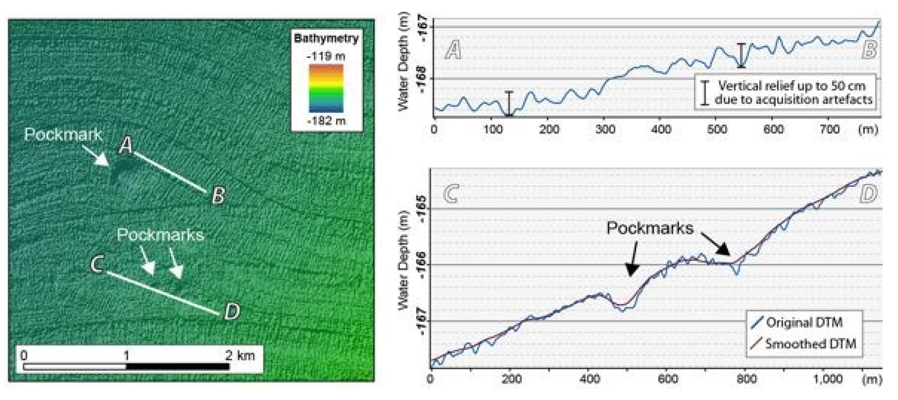
Figure 6.
(A) Example of a small basin initially mapped by the Delineation Tool as a confined depression (contour lines every 1 m); (B) Detail of the raster obtained by applying a High Pass filter followed a Low Pass filter; (C) Black polygons delineate areas of negative values within the filtered dataset (in yellow), which can correspond to either pockmarks or artefacts; (D) Clipped bathymetric dataset based on the delineated polygons; (E) The result of running the Delineation Tool with a clipped bathymetry.

Figure 7.
Example of the delineated outline depending on the choice of the different values of Cutoff Vertical Relief (cut-off VR) and Buffer Distance. Note that the green outline better represents the pockmarks’ limits than the red outline.
Figure 7.
Example of the delineated outline depending on the choice of the different values of Cutoff Vertical Relief (cut-off VR) and Buffer Distance. Note that the green outline better represents the pockmarks’ limits than the red outline.
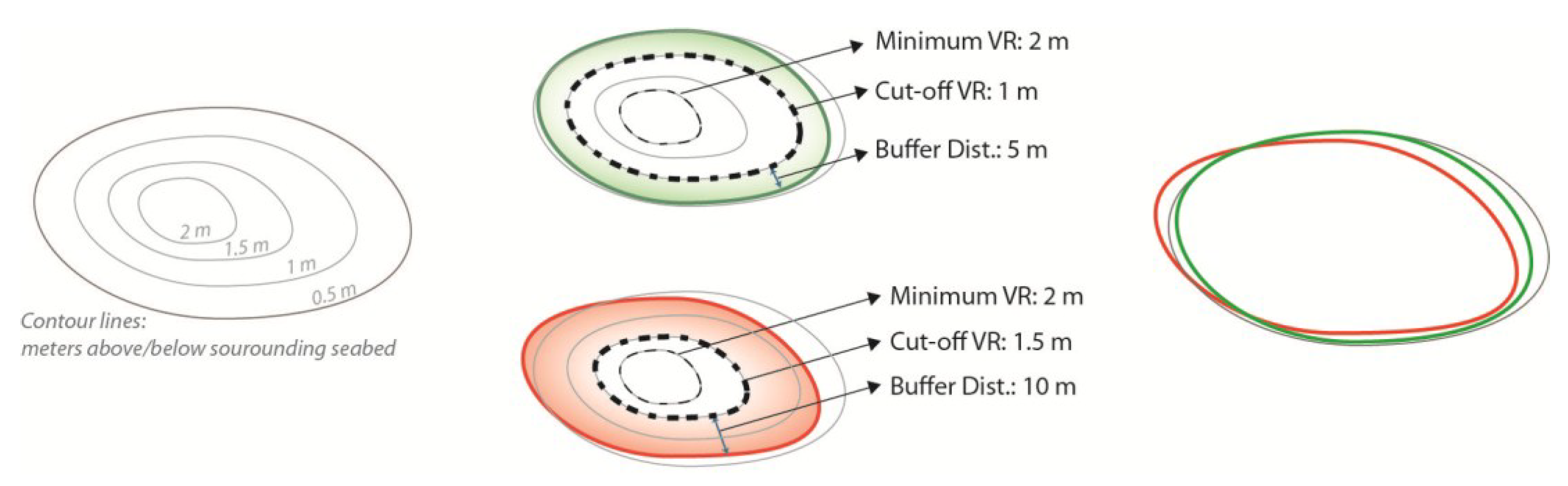
Figure 8.
Schematic representation of two different type of pockmarks profiles and how the position of the mean will lead to lower or higher PI values.
Figure 8.
Schematic representation of two different type of pockmarks profiles and how the position of the mean will lead to lower or higher PI values.
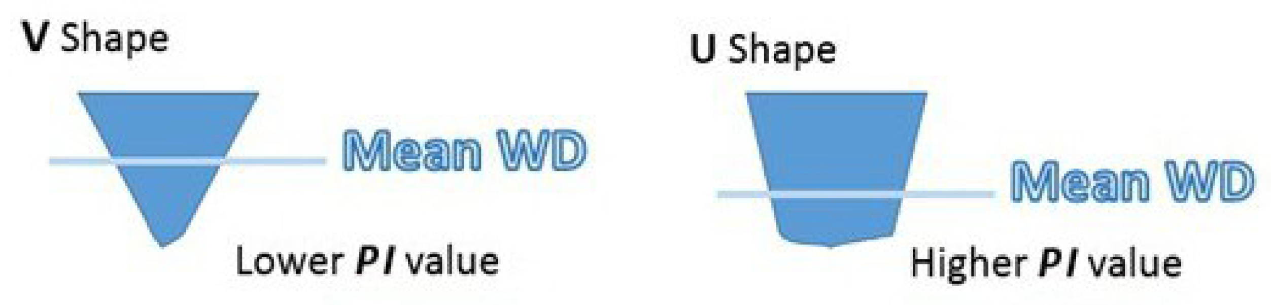
Figure 9.
Pockmark density across the Witch Ground Basin. Survey sites colour coded according to the pockmark density observed. The regional bathymetry shows deeper areas (−150 m) in a darker blue and shallower areas (−90 m) in light blue [9].
Figure 9.
Pockmark density across the Witch Ground Basin. Survey sites colour coded according to the pockmark density observed. The regional bathymetry shows deeper areas (−150 m) in a darker blue and shallower areas (−90 m) in light blue [9].
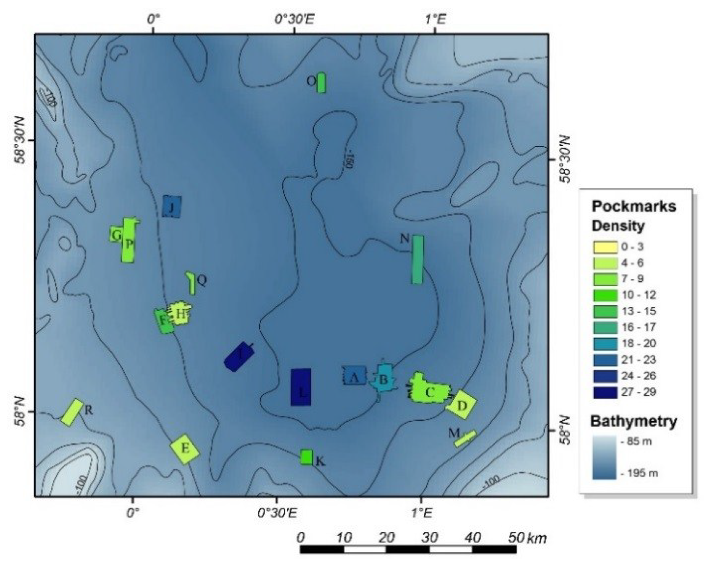
Figure 10.
(A) Box plot of the pockmarks’ vertical relief over individual study areas mapped in the Witch Ground Basin; (B) Vertical relief as a function of Minimum Water Depth.
Figure 10.
(A) Box plot of the pockmarks’ vertical relief over individual study areas mapped in the Witch Ground Basin; (B) Vertical relief as a function of Minimum Water Depth.
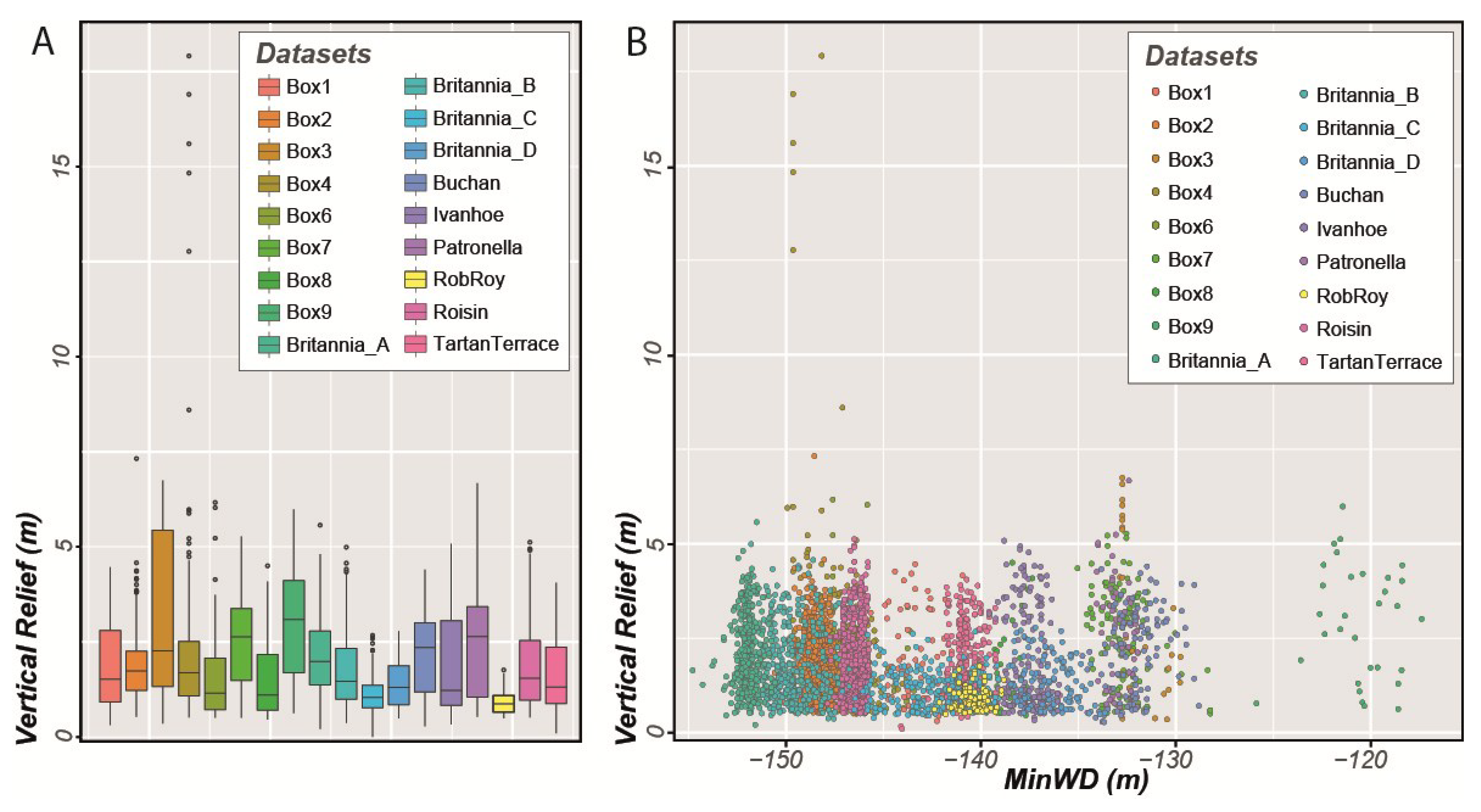
Figure 11.
Vertical Relief as a function of Area in pockmarks with vertical relief lower than eight metres within the Witch Ground Basin. Note that the unusually large pockmarks existent in the Witch Ground Basin are not displayed in this figure.
Figure 11.
Vertical Relief as a function of Area in pockmarks with vertical relief lower than eight metres within the Witch Ground Basin. Note that the unusually large pockmarks existent in the Witch Ground Basin are not displayed in this figure.

Figure 12.
Examples of the initial results from BGS toolbox for SEA 2 Box 4—the pockmarks delineated by the tool are shown in red over a colour-shaded relief map from the southern part of Box 4. Resolution 6 m. Note that manual editing was later required to split the Scanner Pockmark Complex (SPC) into Western Scanner, Eastern Scanner, and adjacent pockmarks.

Figure 13.
Examples of pixel-based terrain attributes from the southern part of SEA2 Box 4. Background data—greyscale shaded relief image of bathymetry data. Pockmark features delineated by the BGS Mapping toolbox are shown in red for reference. All terrain attributes except (B) are coloured according to natural breaks classification and no colour is used for irrelevant classes, where appropriate, to aid visualisation. (A) Slope calculated in ArcGIS Spatial Analyst using standard 3 × 3 rectangular neighbourhood; (B) BPI (integer) using the BTM toolbox using annulus neighbourhood with an inner radius of 1 and an outer radius 5; (C) BPI (floating point) calculated using a 5 × 5 rectangular window—negative BPI values correspond to negative features (depressions) in the seabed, including pockmarks, positive features (BPI value > 0) are not shown. Note that values in the range −0.2–0 (cyan) highlight numerous small artefacts in the data in addition to the shallower portions of pockmarks; (D) Curvature calculated using ArcGIS Spatial Analyst using standard 3 × 3 rectangular neighbourhood—values from −0.3 to 0.6 (close to flat) are not coloured. (E) Minimum Curvature calculated using a 9 × 9 rectangular neighbourhood—values greater than −0.001 are not coloured; (F) Profile curvature calculated using a 15 × 15 rectangular neighbourhood—values greater than −0.0003 are not coloured (flat and positive features). Note that visual interpretation of the results, and the extent to which features and artefacts show up is very dependent on the colour ramp used. These figures are intended as examples only.

Figure 14.
Examples of feature classification using different analysis window size. Background data - greyscale shaded relief image of bathymetry data. Pockmark features delineated by the BGS Mapping toolbox are shown in red for reference. (A) Pit features (yellow) from feature analysis using 9 × 9 rectangular neighbourhood; (B) Pit features (yellow) from feature analysis using 15 × 15 rectangular neighbourhood; (C) Pit features (yellow) from feature analysis using 27 × 27 rectangular neighbourhood; (D) Pit features (yellow) from feature analysis using 51 × 51 rectangular neighbourhood.
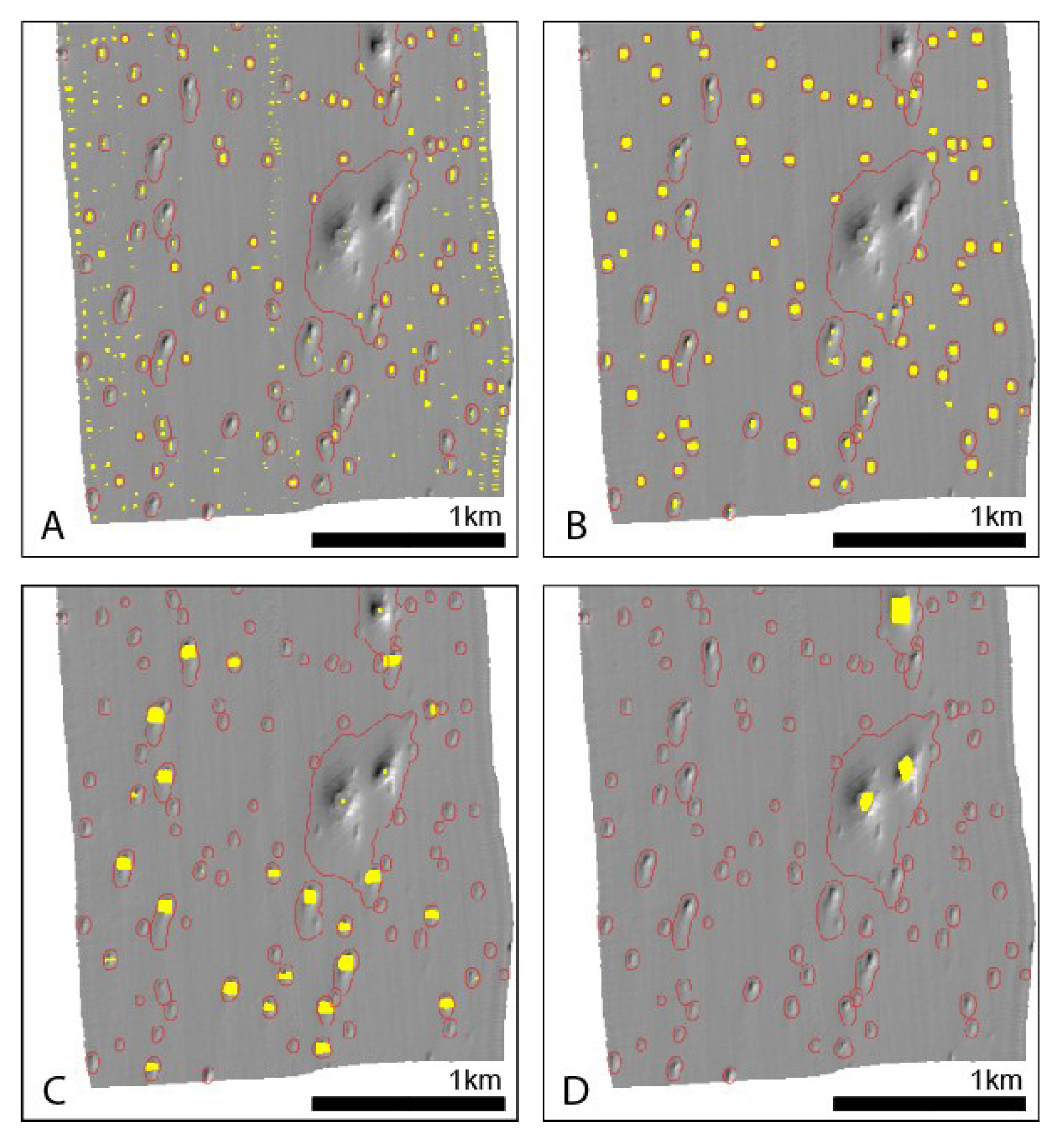
Figure 15.
Detail of the original Malin Deep dataset and the mapping results based on the smoothed bathymetry.
Figure 15.
Detail of the original Malin Deep dataset and the mapping results based on the smoothed bathymetry.
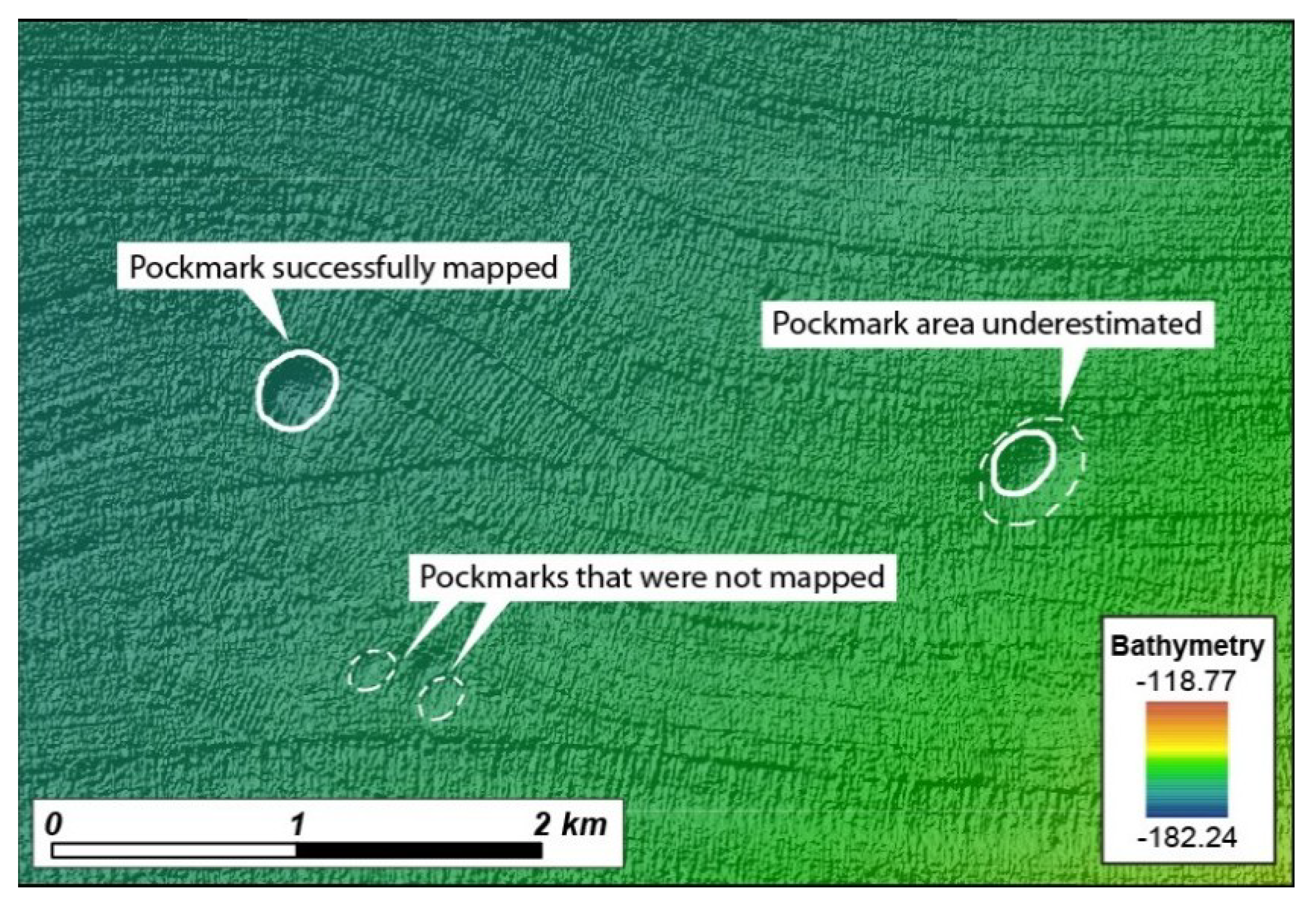
Figure 16.
(A) Location map of the 150 pockmarks mapped with the BGS Seabed Mapping Toolbox (red dots); (B) Vertical Relief as a function of Area for the pockmarks mapped in the Malin Basin.
Figure 16.
(A) Location map of the 150 pockmarks mapped with the BGS Seabed Mapping Toolbox (red dots); (B) Vertical Relief as a function of Area for the pockmarks mapped in the Malin Basin.

Figure 17.
Boxplots for Area, MBG Length, and Vertical Relief for pockmarks mapped in the Malin Basin.
Figure 17.
Boxplots for Area, MBG Length, and Vertical Relief for pockmarks mapped in the Malin Basin.
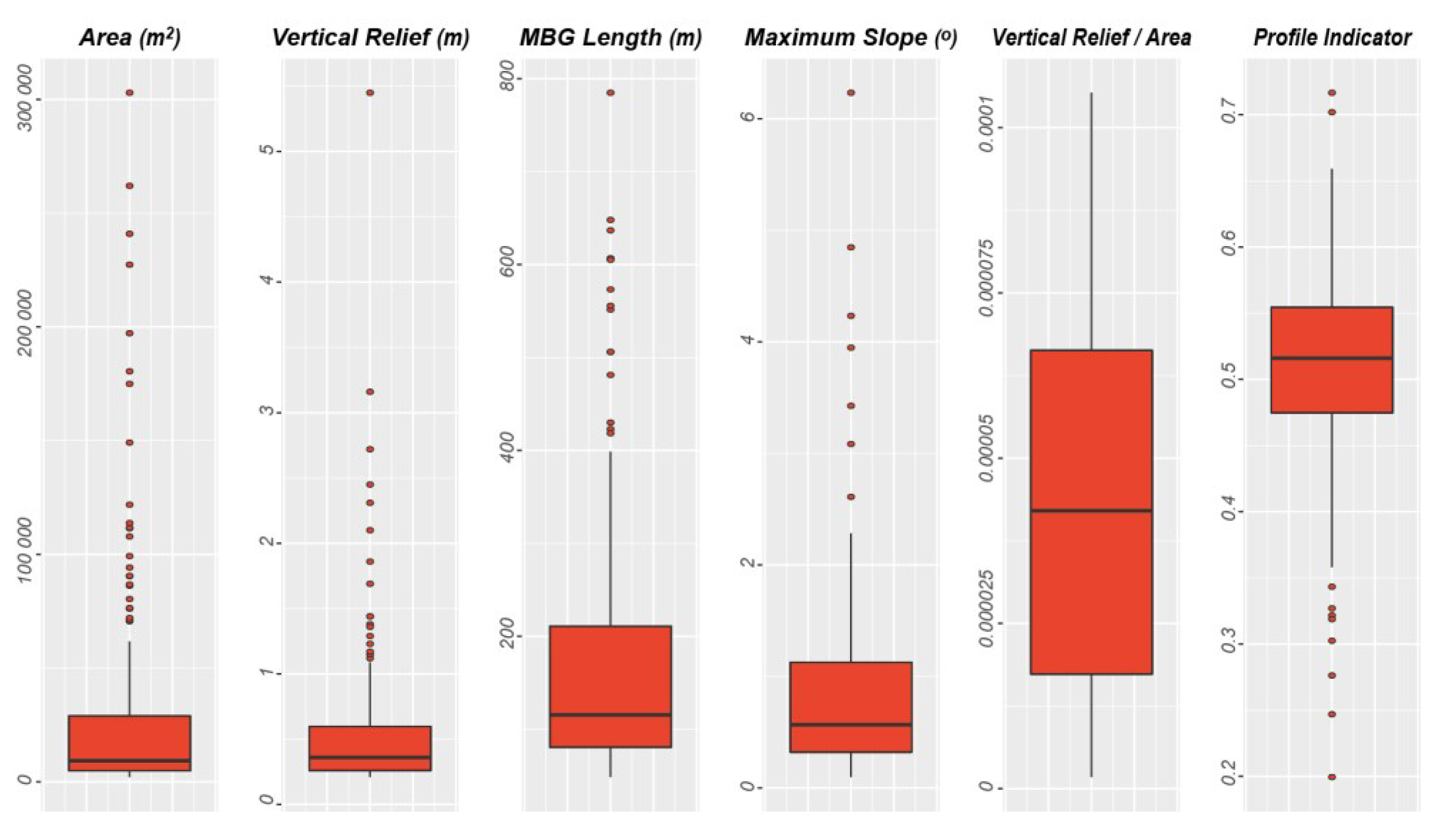
Figure 18.
Malin Deep’s pockmarks distribution based on both manual and semi-automatic mapping.
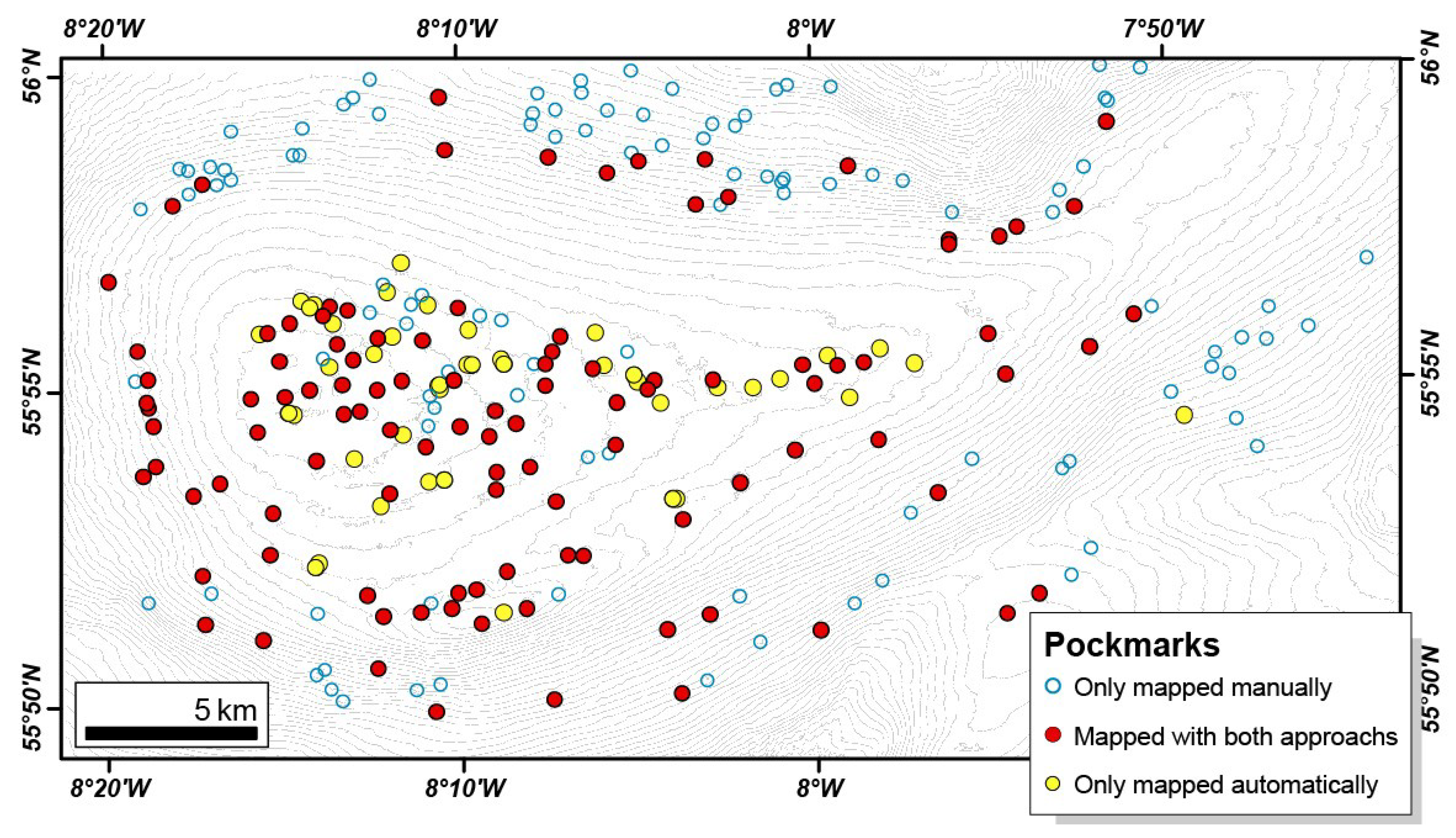
Figure 19.
(Left) Vertical Relief as a function of Area in pockmarks mapped in the Barent Sea’s dataset. Selection of the pockmarks with the higher ratio of VR/A (in cyan); (Right) Detail of the DTM showing the pockmark delineation obtained, with the polygons with the higher ratio of VR/A highlighted on the map view.

Figure 20.
Box plot for the Area, Vertical Relief, MBG Length Vertical Relief/Area ratio, and PI measured for both the single and complex pockmarks mapped.
Figure 20.
Box plot for the Area, Vertical Relief, MBG Length Vertical Relief/Area ratio, and PI measured for both the single and complex pockmarks mapped.
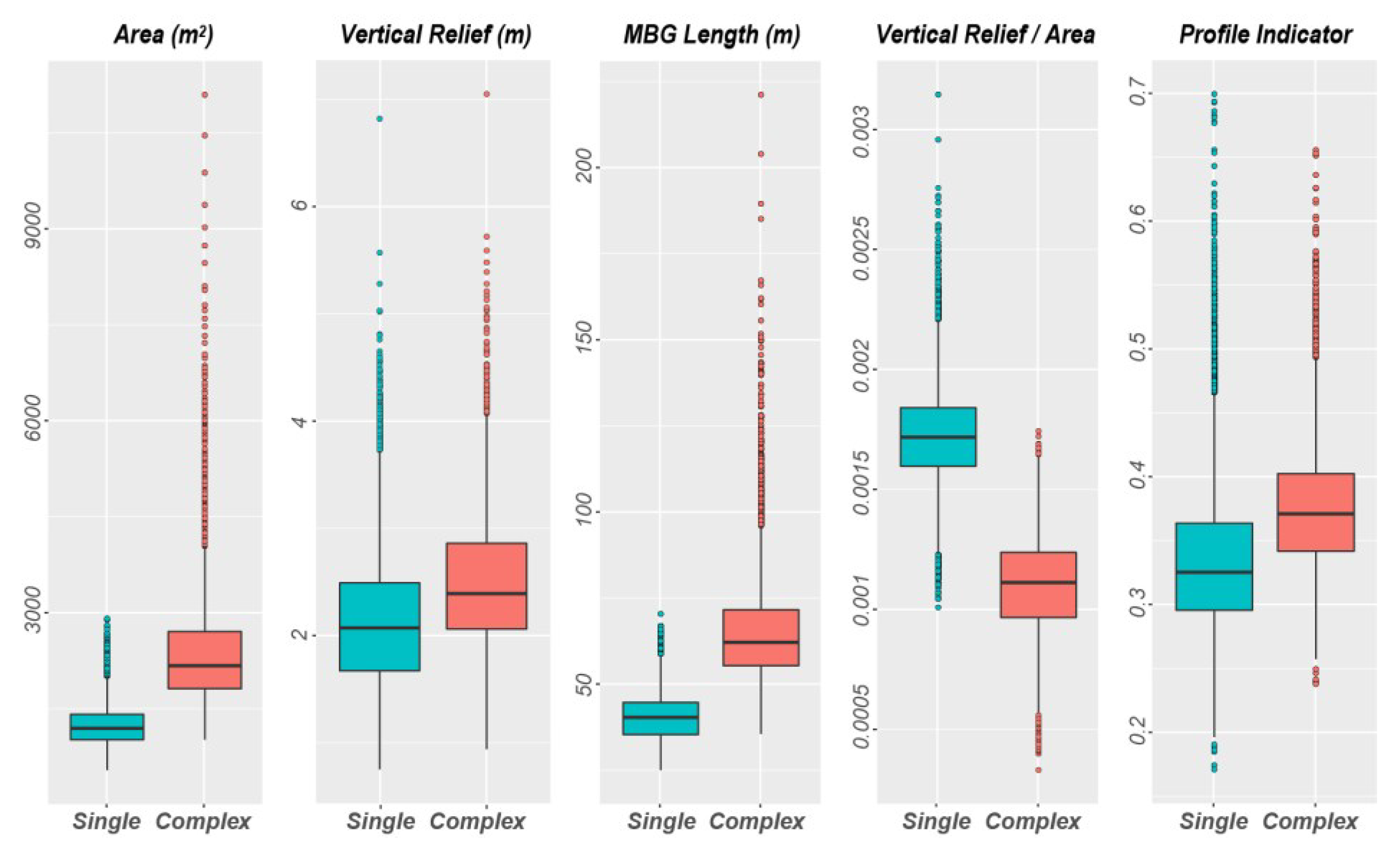
Figure 21.
(A) Stacked histogram of the Vertical Relief values for all mapped pockmarks in the Barents Sea by minimum water depths classes; (B) Internal Vertical Relief versus Minimum Water Depth plot of both single and complex pockmarks.
Figure 21.
(A) Stacked histogram of the Vertical Relief values for all mapped pockmarks in the Barents Sea by minimum water depths classes; (B) Internal Vertical Relief versus Minimum Water Depth plot of both single and complex pockmarks.

Figure 22.
Vertical Relief as a function of Area comparing pockmarks mapped in the three studied regions (Barents Sea: red dots, North Sea: blue dots; and Malin Basin; green dots). Note that the five outlier values from the Witch Ground Basin are not presented here to facilitate better display of the general trends in the remaining data.

Figure 23.
Unsorted correlograms showing the relationships between key pockmark metrics for the three studied regions.
Figure 23.
Unsorted correlograms showing the relationships between key pockmark metrics for the three studied regions.

Figure 24.
Unsorted correlograms showing the different relationships between key pockmark metrics for the two types of pockmarks found in the Barents Sea. Note the higher value of correlation between Area and Vertical Relief for the single pockmarks.
Figure 24.
Unsorted correlograms showing the different relationships between key pockmark metrics for the two types of pockmarks found in the Barents Sea. Note the higher value of correlation between Area and Vertical Relief for the single pockmarks.

Figure 25.
Pockmark density and distribution map of the Barents Sea study area, obtained using the mapping results from the BGS Seabed Mapping Toolbox.
Figure 25.
Pockmark density and distribution map of the Barents Sea study area, obtained using the mapping results from the BGS Seabed Mapping Toolbox.


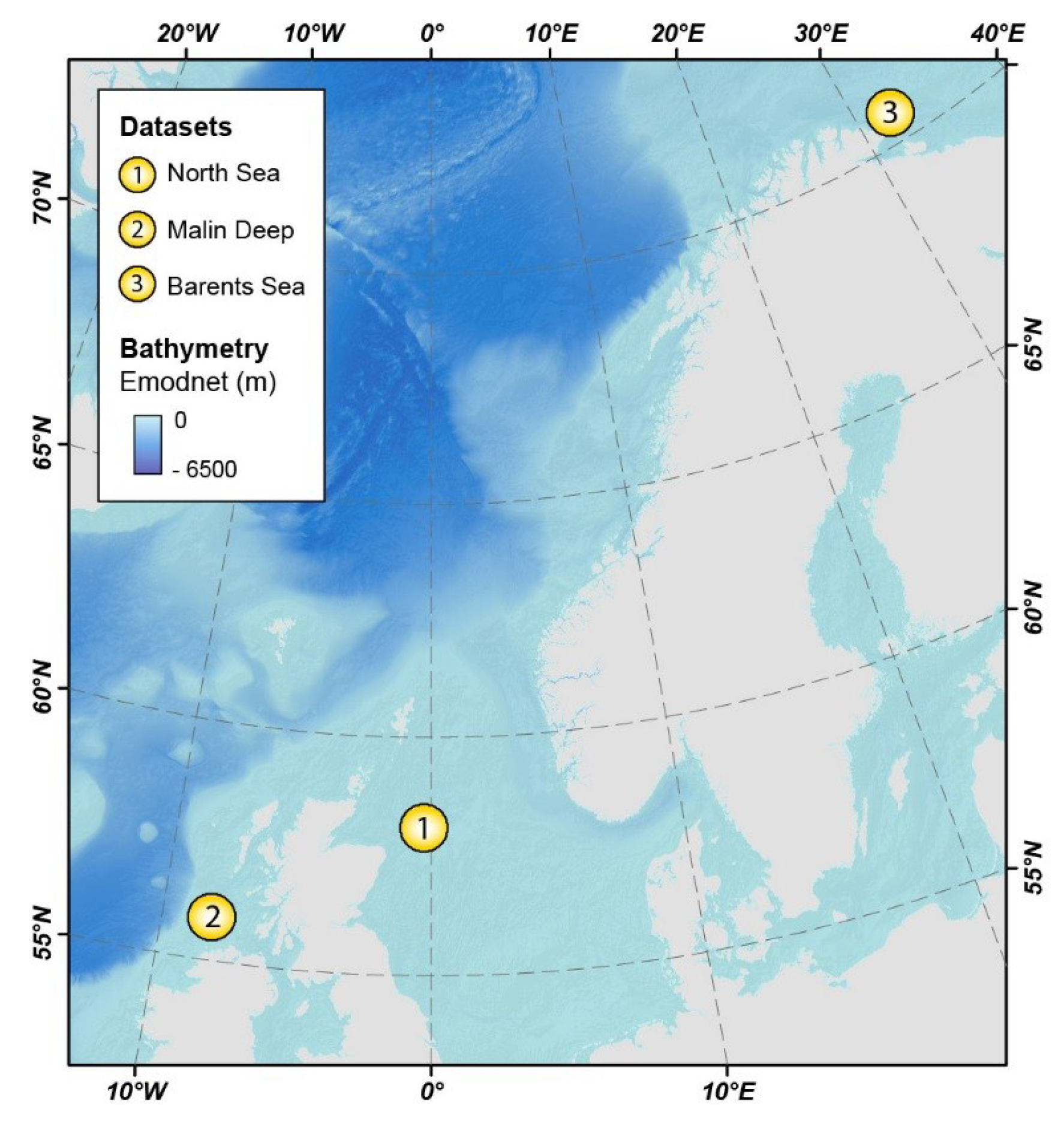
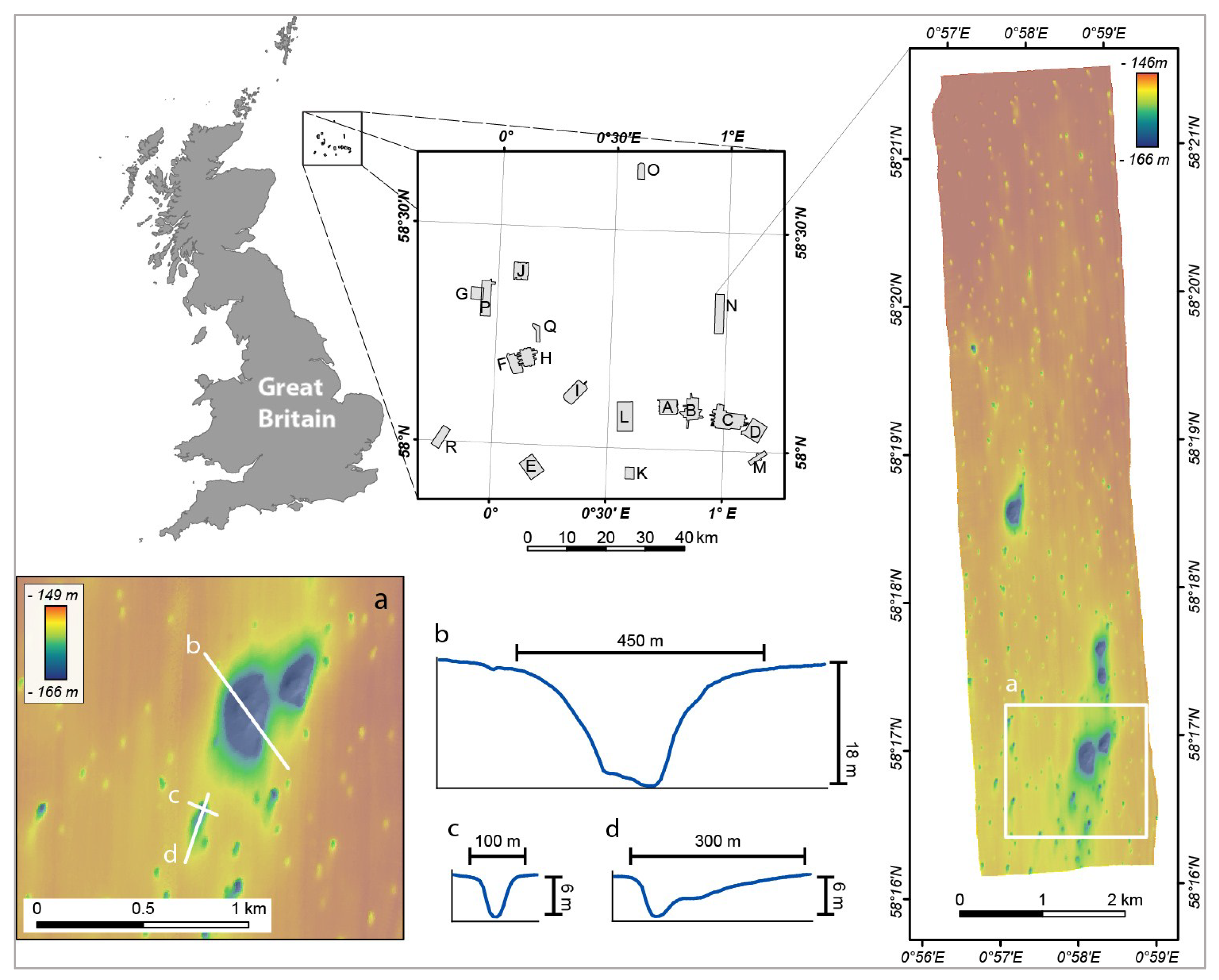
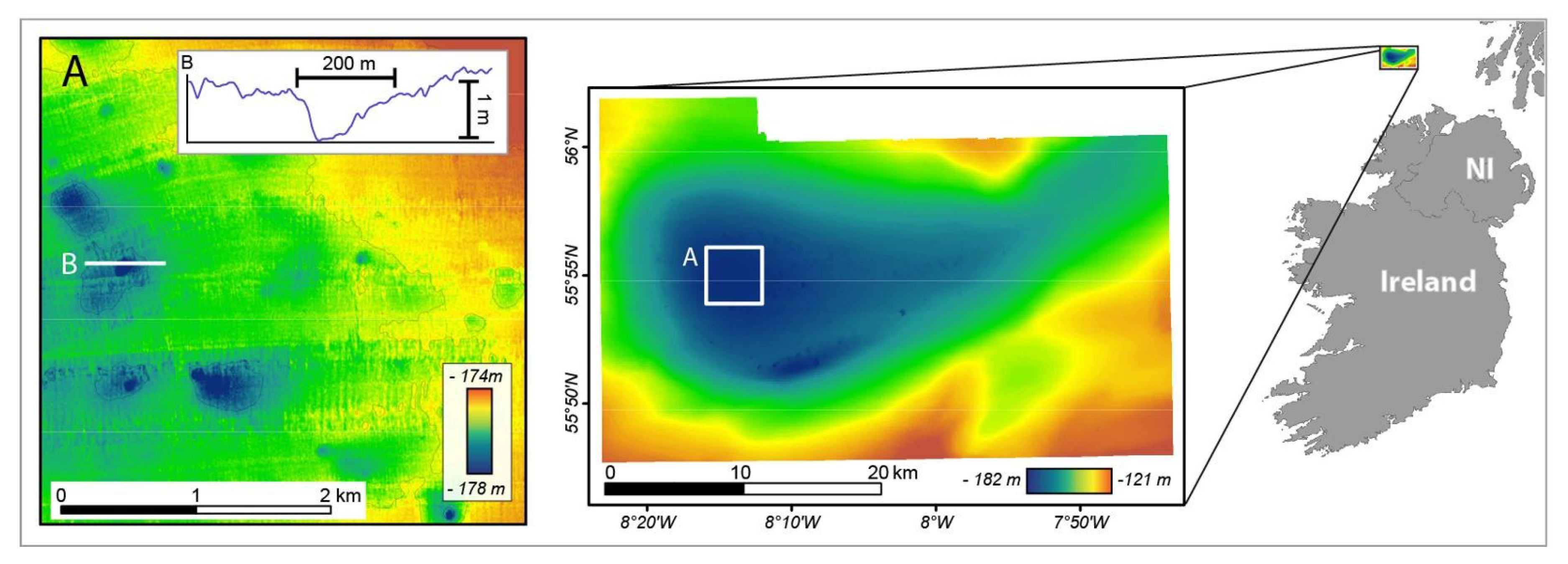
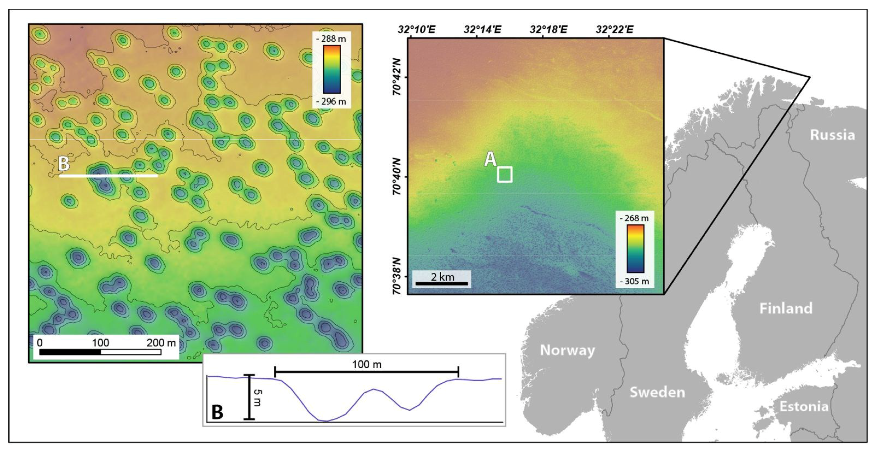
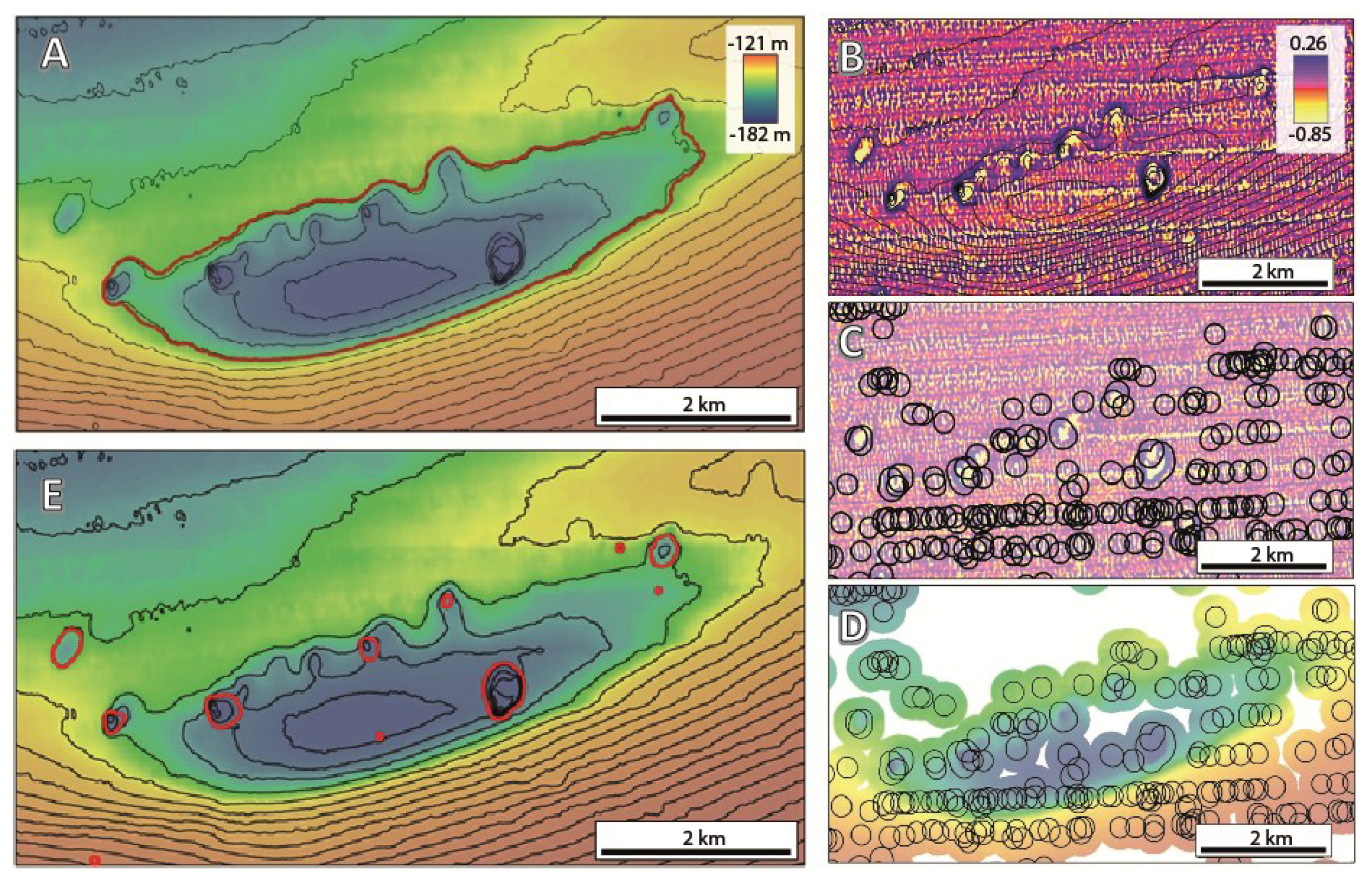
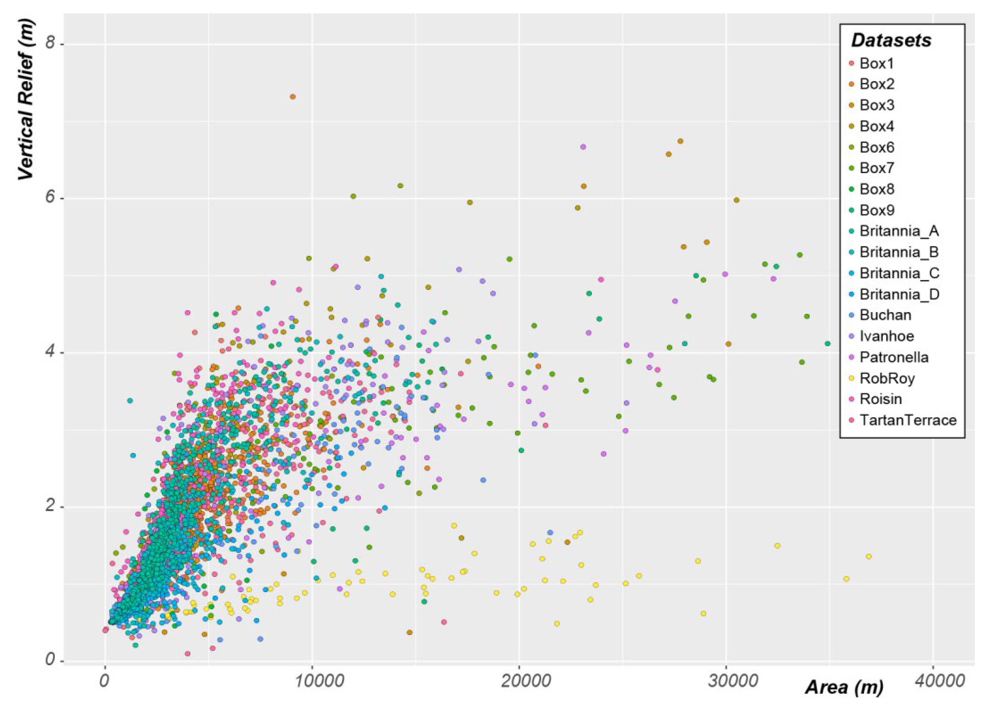
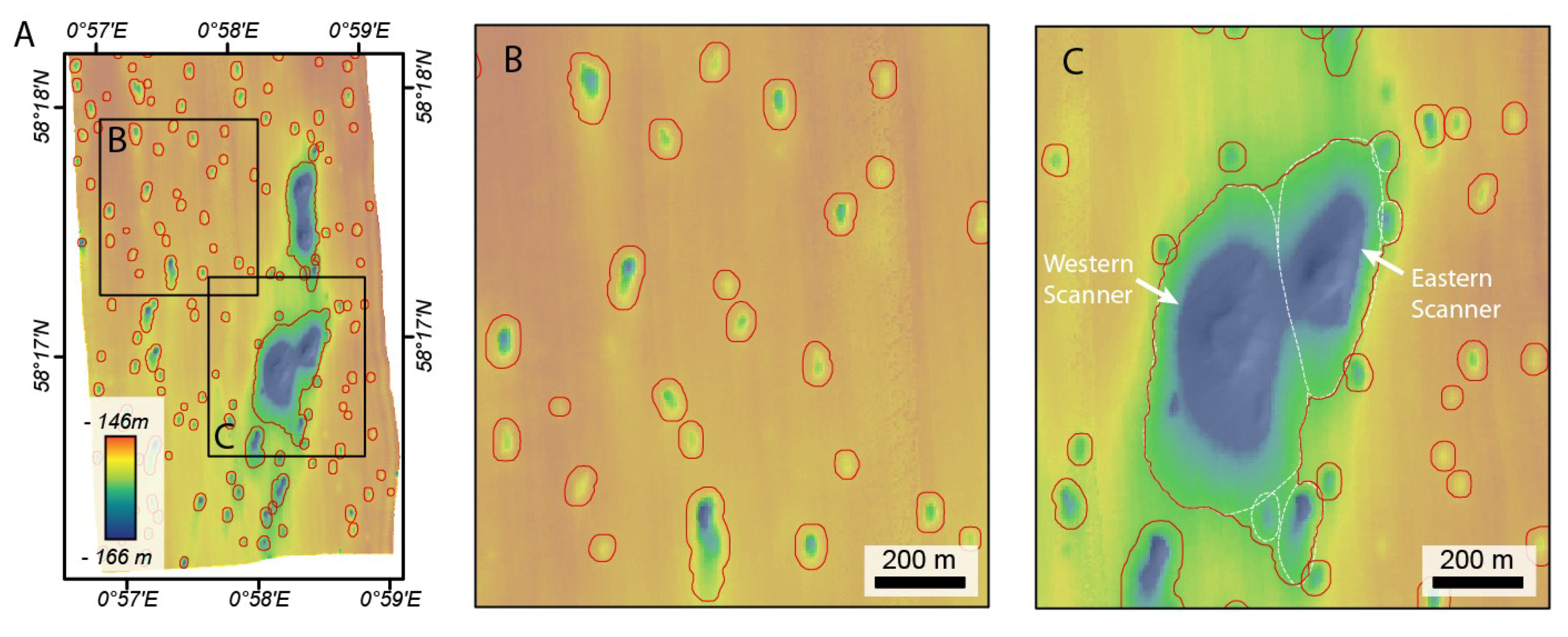
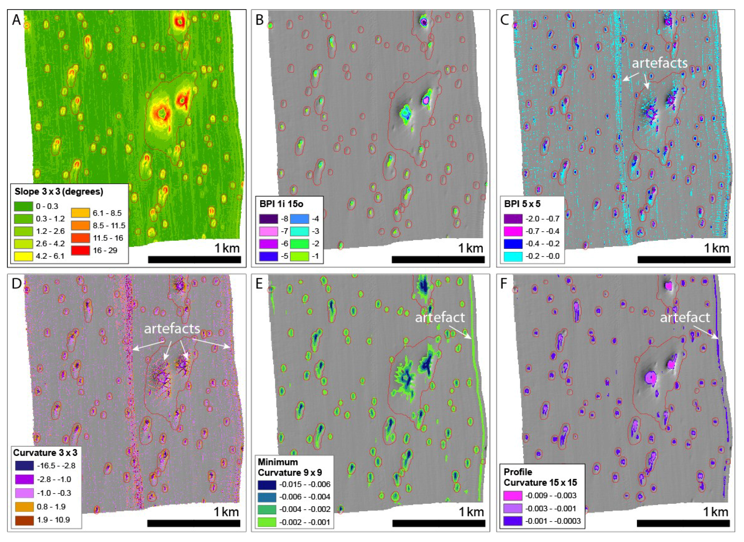
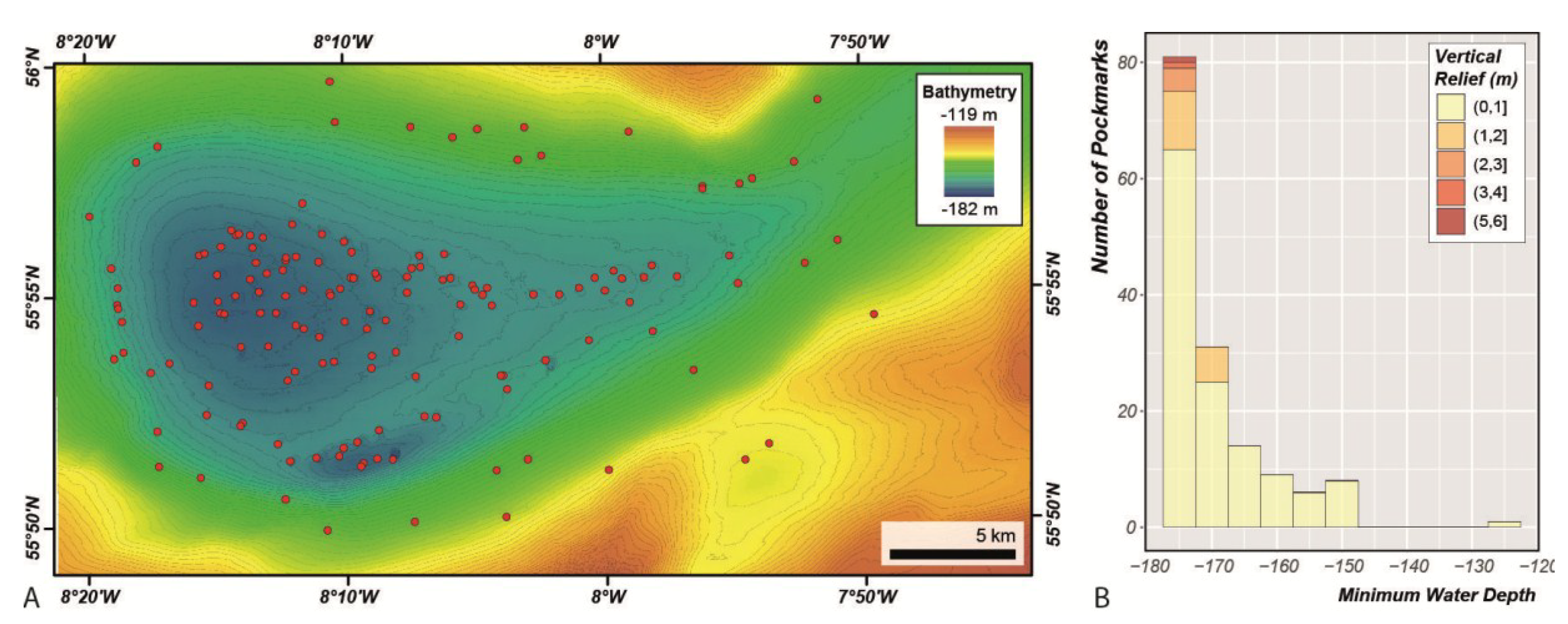
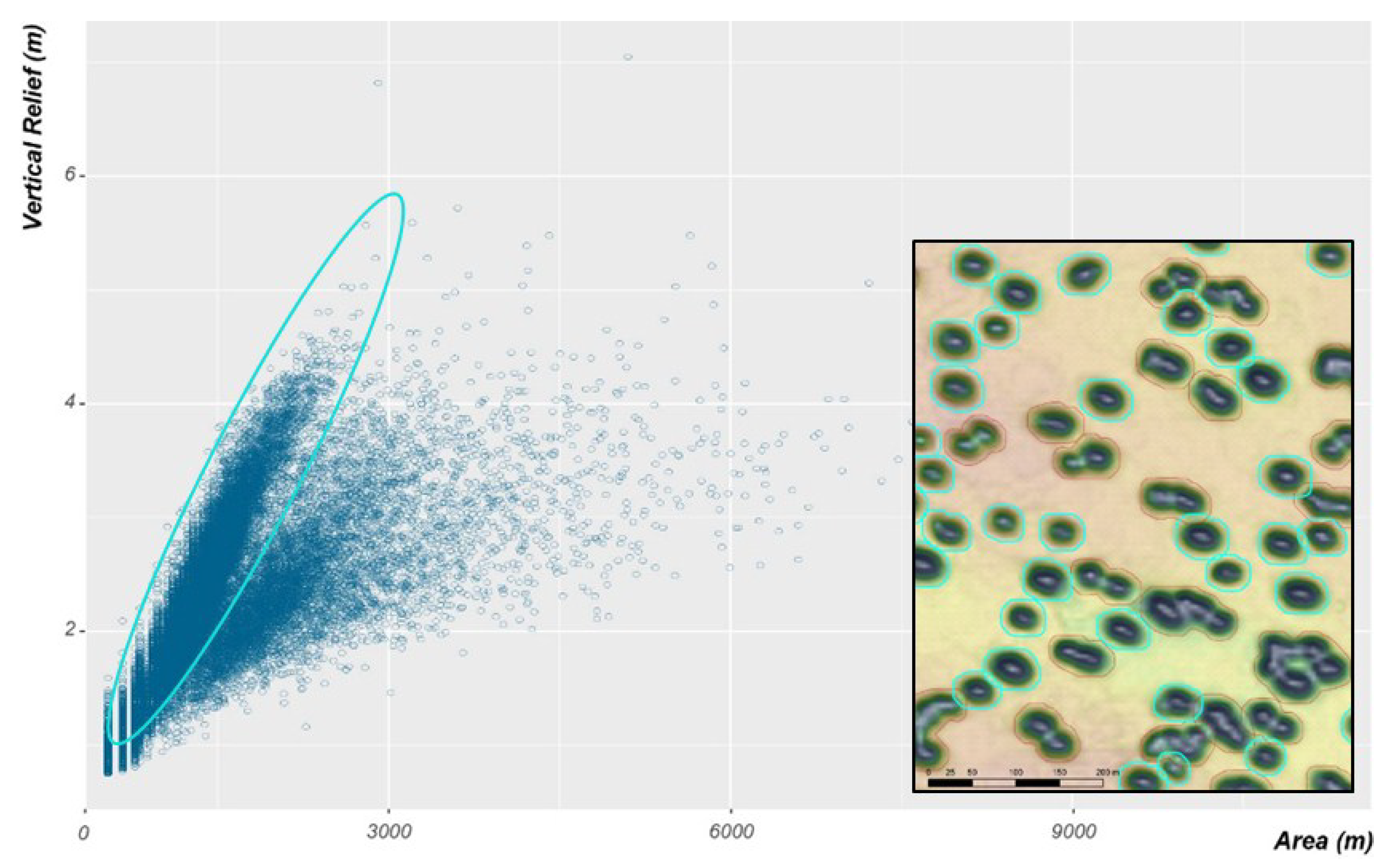
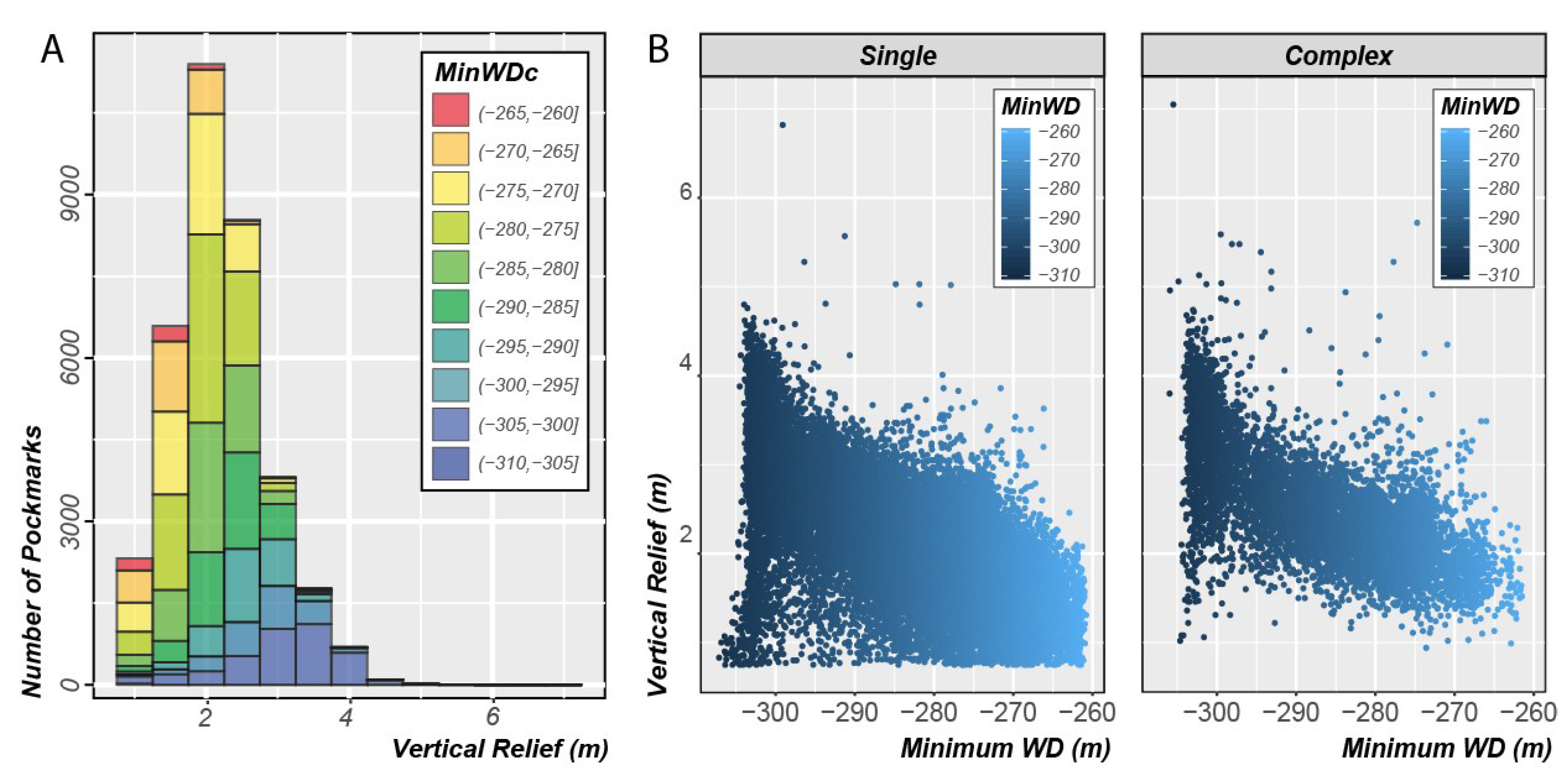
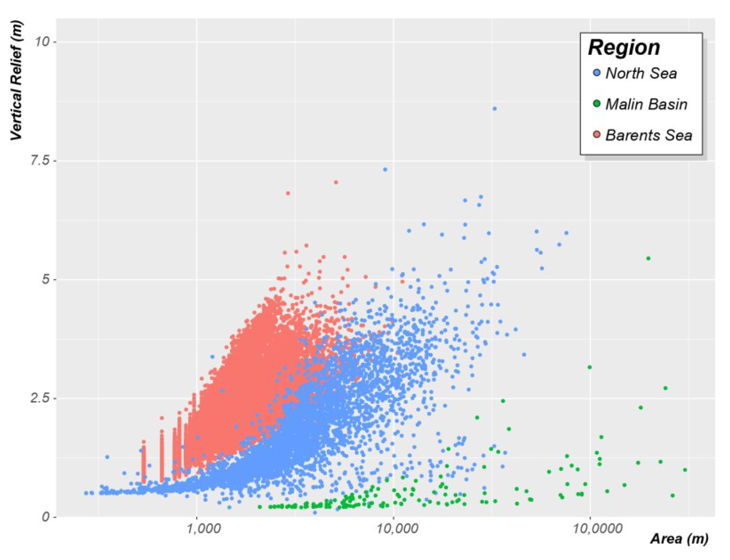
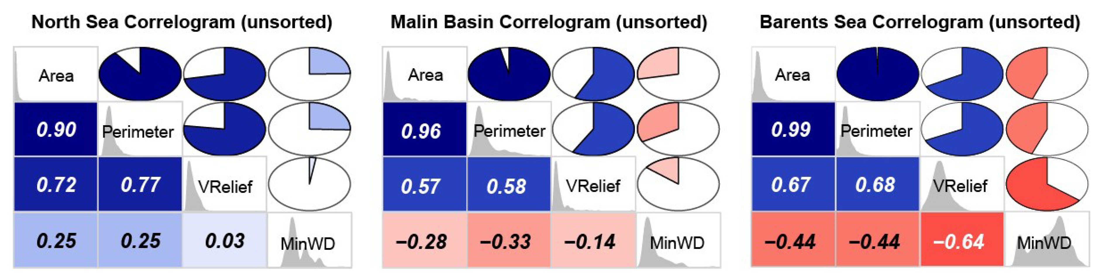
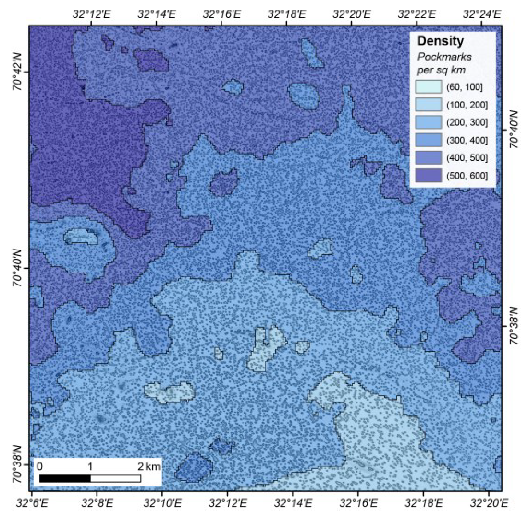
Table 1.
Summary of pixel-based approaches to pockmark mapping in SEA2 Box 4, Witch Ground Basin.
| Terrain Attribute | Analysis Scale Used (Pixel n × n Neighbourhood, Except BPI (BTM Toolbox) | Method |
|---|---|---|
| Single scale slope | n = 3 | Standard 3 × 3 curvature from ArcGIS 10.4.1 Spatial Analyst [20] |
| Multiple scale slope | n = 5, 9, 15 | GRASS module r.param.scale via QGIS 2.18.11 based on the methods of [21]. |
| Multiple scale Bathymetric Position Index (BPI) | Inner radius 1, 3 Outer radius 5, 15 | Fine_scale BPI using the BTM toolbox [22]. Annulus neighbourhood with selected inner and outer radius. Produces integer output. |
| Multiple scale BPI (modified) | n = 5, 9, 15 | This modified version of BPI implemented in ArcGIS Spatial Analyst raster calculator produces a floating-point grid. The computation is similar to that presented by [23] but uses a rectangular neighbourhood to facilitate using the same neighbourhood as other analyses. |
| Curvature | n = 3 | Standard, 3 × 3 curvature from ArcGIS 10.4.1 Spatial Analyst [24]. |
| Multiple scale minimum curvature Multiple scale profile curvature | n = 5, 9, 15 n = 5, 9, 15 | Multiple scale curvature calculated using GRASS module r.param.scale via QGIS 2.18.11 which is based on the methods of [21]. |
| Multiple scale feature classification | n = 9, 15, 27, 51 | Multiple scale feature classification calculated using GRASS module r.param.scale via QGIS 2.18.11 from r.param.scale [21]. |
Table 2.
Table of thresholds used for three study areas: Cut-off Vertical Relief (Cut-off VR), Minimum Vertical Relief (Min VR), Minimum Width (Min Width), Minimum Size Ratio (Min W/L), and Buffer Distance. Note that North Sea’s pockmarks were mapped with the first version of the delineation tool that used a different set of thresholds.
| Study Area | Cut-off VR | Min VR | Min Width | Min W/L | Buffer Distance |
|---|---|---|---|---|---|
| North Sea | 0.5 m | --- | --- | 0.2 | 7.5 m |
| Malin Basin | 0.2 m | 0.2 m | 40 m | 0.2 | 80 m |
| Barents Sea | 0.75 m | 0.75 m | 4 m | 0.2 | 10 m |
Table 3.
Number of depressions mapped (N), mean area (μ Area), mean width (μ Width), mean length (μ Length), mean of the ratio between width and length (μ W/L), and vertical relief (μ VR) from the depressions classified as single and complex pockmarks, respectively.
Table 3.
Number of depressions mapped (N), mean area (μ Area), mean width (μ Width), mean length (μ Length), mean of the ratio between width and length (μ W/L), and vertical relief (μ VR) from the depressions classified as single and complex pockmarks, respectively.
| N | μ Area | μ Width | μ Length | μ W/L | μ VR | |
|---|---|---|---|---|---|---|
| Single Pockmarks | 28,014 | 1223 | 15.5 | 19.4 | 0.82 | 2.12 |
| Complex Pockmarks | 7223 | 2386 | 24.6 | 45.4 | 0.5 | 2.5 |
© 2018 by the authors. Licensee MDPI, Basel, Switzerland. This article is an open access article distributed under the terms and conditions of the Creative Commons Attribution (CC BY) license (http://creativecommons.org/licenses/by/4.0/).
Share and Cite
MDPI and ACS Style
Gafeira, J.; Dolan, M.F.J.; Monteys, X. Geomorphometric Characterization of Pockmarks by Using a GIS-Based Semi-Automated Toolbox. Geosciences 2018, 8, 154. https://doi.org/10.3390/geosciences8050154
AMA Style
Gafeira J, Dolan MFJ, Monteys X. Geomorphometric Characterization of Pockmarks by Using a GIS-Based Semi-Automated Toolbox. Geosciences. 2018; 8(5):154. https://doi.org/10.3390/geosciences8050154
Chicago/Turabian StyleGafeira, Joana, Margaret F. J. Dolan, and Xavier Monteys. 2018. "Geomorphometric Characterization of Pockmarks by Using a GIS-Based Semi-Automated Toolbox" Geosciences 8, no. 5: 154. https://doi.org/10.3390/geosciences8050154
Note that from the first issue of 2016, this journal uses article numbers instead of page numbers. See further details here.