Investigation of the Effect of Debris-Induced Damage for Constructing Tsunami Fragility Curves for Buildings

1
EngD Researcher, EPICentre, University College London, London WC1E 6BT, UK
2
EPICentre, University College London (UCL), London WC1E 6BT, UK
*
Author to whom correspondence should be addressed.
Geosciences 2018, 8(4), 117; https://doi.org/10.3390/geosciences8040117
Submission received: 30 September 2017
/
Revised: 11 March 2018
/
Accepted: 12 March 2018
/
Published: 31 March 2018
(This article belongs to the Special Issue Interdisciplinary Geosciences Perspectives of Tsunami)
Abstract
:Catastrophe models quantify potential losses from disasters, and are used in the insurance, disaster-risk management, and engineering industries. Tsunami fragility and vulnerability curves are key components of catastrophe models, providing probabilistic links between Tsunami Intensity Measures (TIMs), damage and loss. Building damage due to tsunamis can occur due to fluid forces or debris impact; two effects which have different implications for building damage levels and failure mechanisms. However, existing fragility functions are generally derived using all available damage data for a location, regardless of whether damage was caused by fluid or debris effects. It is therefore not clear whether the inclusion of debris-induced damage introduces bias in existing functions. Furthermore, when modelling areas likely to be affected by debris (e.g., adjacent to ports), it is not possible to account for this increased likelihood of debris-induced damage using existing functions. This paper proposes a methodology to quantify the effect that debris-induced damage has on fragility and vulnerability function derivation, and subsequent loss estimates. A building-by-building damage dataset from the 2011 Great East Japan Earthquake and Tsunami is used, together with several statistical techniques advanced in the field of fragility analysis. First, buildings are identified which are most likely to have been affected by debris from nearby ‘washed away’ buildings. Fragility functions are then derived incorporating this debris indicator parameter. The debris parameter is shown to be significant for all but the lowest damage state (“minor damage”), and functions which incorporate the debris parameter are shown to have a statistically significant better fit to the observed damage data than models which omit debris information. Finally, for a case study scenario simulated economic loss is compared for estimates from vulnerability functions which do and do not incorporate a debris term. This comparison suggests that biases in loss estimation may be introduced if not explicitly modelling debris. The proposed methodology provides a step towards allowing catastrophe models to more reliably predict the expected damage and losses in areas with increased likelihood of debris, which is of relevance for the engineering, disaster risk-reduction and insurance sectors.
1. Introduction
Tsunami have the potential to cause huge economic and financial losses, as demonstrated by the 2011 Great East Japan Earthquake and Tsunami (referred to throughout as the 2011 Japan Tsunami), which cost the lives of over 18,500 people (National Police Agency of Japan, 2017). Tsunami fragility functions are a family of cumulative distribution functions (Figure 1) that provide the probability of a given type of building exceeding specified damage states (each individual curve represents a specific damage state) for a given value of a Tsunami Intensity Measure (TIM, e.g., inundation depth). Vulnerability functions are generally derived from fragility functions, and are cumulative distribution functions that relate expected human or financial losses to a TIM. Vulnerability functions are a key component of catastrophe models, and so are vital for land-use and emergency planning as well as human and financial loss estimation, for the purposes of mitigation and transfer of tsunami risk.
Tsunami-induced building damage can arise due to water ingress (damage to building contents and non-structural elements), fluid forces (hydrostatic and hydrodynamic) and debris effects (impact and damming). Debris effects are a significant source of building damage, yet are seldom explicitly modelled in tsunami fragility and vulnerability functions. Debris effects on buildings include:
- Impact from large water-borne objects (e.g., cars, ships, shipping containers, trees, building fragments etc. Figure 2a). A function of debris mass, velocity and contact duration (hardness);
- Increase in flow viscosity/density due to collected smaller debris/sediment (Figure 2b);
- Damming (filling of openings with debris, increasing the effective area experiencing lateral load, Figure 2b).
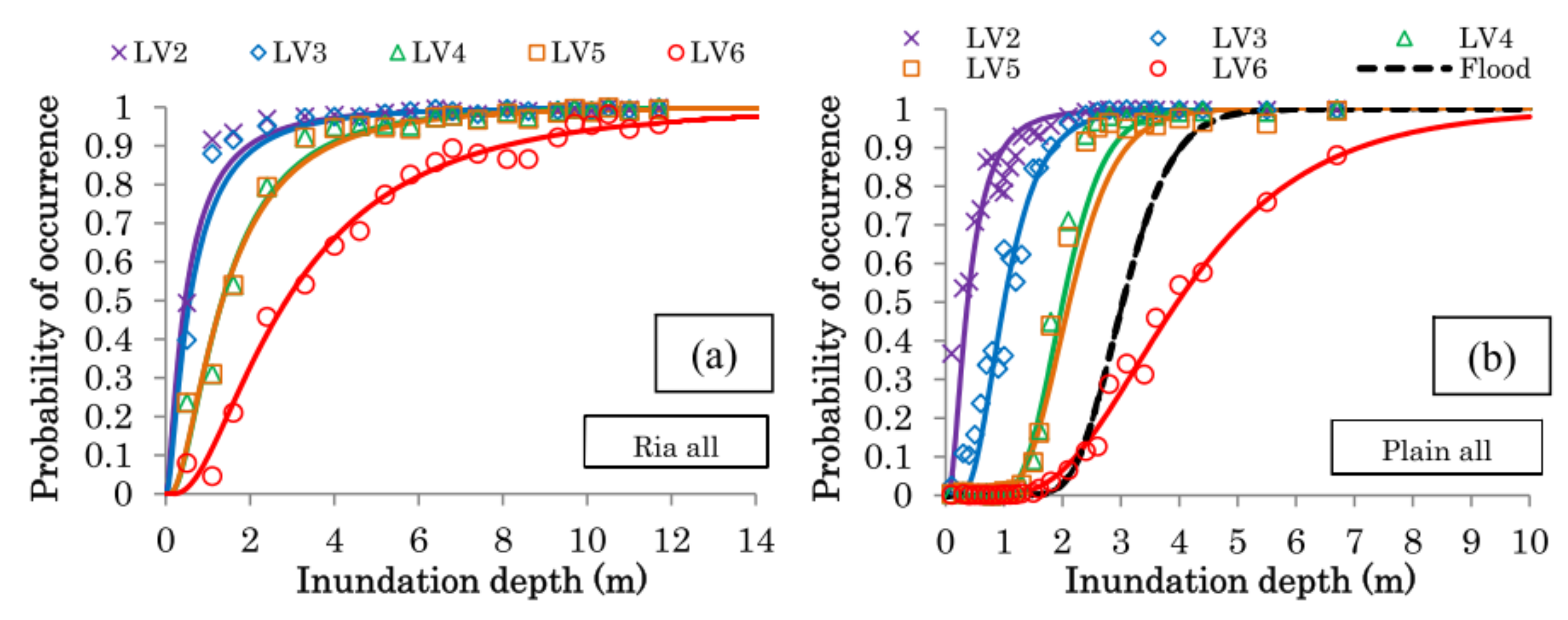
Compared to seismic studies, few fragility functions for buildings affected by tsunami exist, and studies collating these functions [1,2] show that the vast majority have been based solely on data collected during the aftermath of the 2011 Japan Tsunami. Empirical fragility curves are very specific to the building type and flow and debris conditions from where the data was taken [3]. For example, Figure 1 shows very different fragility functions derived from damage data from mountainous and coastal areas of the same city affected by the 2011 Japan Tsunami. These differences stem mainly from the differing flow conditions experienced over these different topographies, rather than from significant differences in building composition. These graphs suggest either that the TIM selected might not be appropriate to fully describe the flow conditions, or that significantly different levels of debris impact are at play in these different geographical areas. Without further clarity, as they stand, it is clear that these empirical fragility functions are highly location-specific.
Various TIMs have been used in recent fragility studies to describe flow conditions, such as depth, velocity and hydrodynamic force [5,6,7], and Macabuag et al. [8] present a methodology for selecting the optimum TIM for a given dataset. However, TIMs in existing fragility studies rarely account explicitly for the debris-induced damage [1,2], and it has not yet been investigated whether this omission introduces a significant bias (systematic error) in the prediction of tsunami damage or loss. Charvet et al. [9] presents initial steps to address this issue by generating fragility functions considering that debris is mostly composed of the remains of collapsed buildings, and as such designates buildings as having been affected by debris if they are within a given distance (distances from 10 m to 150 m are tried) of a building that has been washed away. However, this method both ignores non-building sources of debris (cars, ships, shipping containers, trees etc.), and does not make any allowance for the size or number of collapsed buildings. For example, one small, nearby collapsed structure is considered to be as much a driver of debris damage as several large collapsed structures. The current study proposes to extend this work by also considering the number of nearby collapsed buildings.
Given the needs highlighted above, this paper presents a preliminary investigation to address the following research questions:
- Is bias (systematic error) observed in fragility functions which do not explicitly model the presence of debris in tsunami inland flow?
- Can a reliable and accurate estimation of debris effects be incorporated into fragility function derivation?
- What effect does consideration of debris have on financial loss estimation?
To address the above research questions, this study extends the preliminary work conducted in [10] to examine the effect of debris in more detail and to consider the impact that including debris-effects in models has on loss estimation. Note that a reliable or accurate method for identifying debris impact is a significant challenge requiring further research, and as such is not the main focus of the current study, which will make assumptions to determine debris impact. The study instead focuses on presenting a methodology to conduct sensitivity analyses to determine the effect of debris impact on fragility and vulnerability curve derivation (so identifying bias in current studies), and to model more reliably the expected damage in areas with increased likelihood of debris. The proposed methodology is presented in Section 2, a detailed building-by-building damage dataset and associated tsunami inundation model from the 2011 Japan Tsunami is presented in Section 3, and the proposed methodology is applied to this case-study dataset in Section 4. Finally, the results and their implications for fragility analysis using observational data from past tsunami are discussed.
2. Proposed Methodology
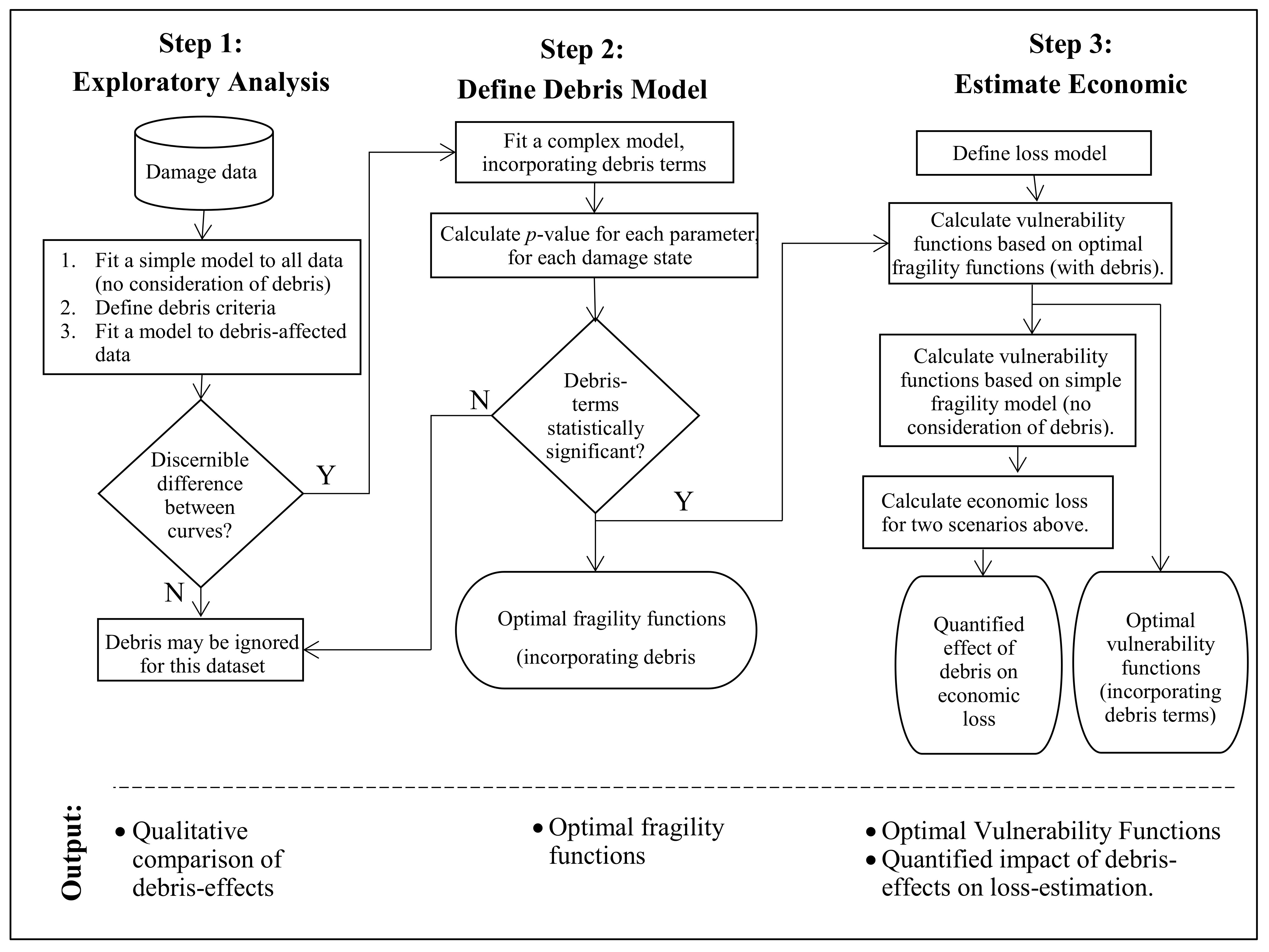
To address the research questions posed in the previous section, a three-step methodology is developed. In the first step, an exploratory analysis is carried out to identify buildings that have been impacted by debris, with a sensitivity study carried out to check the influence of assumptions made on the resulting fragility functions. In the second step, it is investigated whether the addition of a debris term in the fragility functions leads to a statistically significantly better fit to the data. In the third step, vulnerability functions are derived from the fragility functions so as to estimate economic loss for the case study locations, and a comparison is made between estimates from functions which do and do not incorporate a debris term. The three steps are shown in Figure 3, described in more detail in what follows, and demonstrated for a case study dataset in Section 4.
2.1. Step 1: Exploratory Analysis of Debris-Induced Bias
A major source of large debris within tsunami inland flow is from collapsed buildings [9]. Therefore, a very simple assumption is made to identify whether buildings have been affected by debris impact or not: buildings in close proximity to collapsed buildings are assumed to be affected by debris impact. A regular grid is applied to the case study location, and the total footprint area of all “washed away” buildings is calculated for each grid square. If this area exceeds a threshold proportion of the total building footprint area for that grid all buildings of that grid square are deemed to have been affected by debris and so are removed from the dataset. It is highlighted that although this method still ignores non-building sources of debris (cars, ships, shipping containers, trees etc.), it is an improvement on that presented in [9] as it considers the size and number of nearby collapsed buildings.
To assess the sensitivity of this definition of debris impacted buildings to the threshold definition, fragility functions are developed for the complete dataset (i.e., without considering debris) and compared to those developed for buildings assumed to have/have not been affected by debris. A comparison of these functions is used to indicate whether the ignoring of debris-effects may introduce systematic bias.
Key to the empirical fragility assessment is the construction of a statistical model which fits the data best [11]. Fragility curves corresponding to each damage state (index i) are determined by assigning a damage response indicator, damage state (DS), to each building (index j), which is considered to follow a multinomial distribution (termed the “random component” of the model). Each building is also assigned a TIM value, xj. In Macabuag et al. [8], the comparison of various statistical models showed the advantages of using parametric models and in particular the Generalized Linear Model (GLM). GLMs relate the mean of a response variable (the probability of damage state exceedance, P(DS ≥ DSi) to the explanatory variables (xj) (with this relationship often termed the “systematic component” of the model) via an arbitrary link function. Macabuag et al. [8] also introduces Cumulative Link Models (CLMs), which recognize that the damage is an ordinal categorical variable so using all available information regarding the data in the database to form a single model (rather than separate GLMs for each damage state, [12]). For the example of a probit link function (the inverse standard cumulative normal distribution) the components of a CLM are shown in (1) and (2), where β0 and β1 are the unknown regression parameters (i.e., intercept and slope, respectively) estimated by a maximum likelihood optimisation algorithm.
| Random Component | (1) | ||
| Systematic Component | (2) |
Note that many existing studies fit models to the logarithm of the TIM (ln|xj|) [1] so as to force the fragility functions through the origin. This is desirable as it is expected that when the TIM is zero, the probability of damage is also zero. This practice will also therefore be conducted for all models in this study.
Guidelines by the Global Earthquake Model (GEM) for the fragility assessment of building in earthquake-prone areas [11] recommend that uncertainty quantification be conducted using bootstrap methods. It is therefore proposed that 5th and 95th-percentile bootstrap confidence intervals should be constructed for fragility functions in this methodology based on 1000 iterations.
2.2. Step 2: Quantifying the Effect of Debris in Fragility Function Derivation
To address research question 2, the effect of debris on fragility function derivation is quantified by the addition of a debris term in the fragility functions, and then testing of these terms to identify whether they lead to a statistically significantly better fit to the data.
The significance of including debris data in the model is investigated by forming a more complex model which includes a binary debris indicator variable, debrisj, indicating whether or not the building has been affected by debris (3) (i.e., debrisj = 1 for all buildings within grid squares which have a ratio of washed away footprint area to total area above the threshold percentage). The parameter β2,i in Equation (3) adjusts the intercept of the model and Equation (4) includes a fourth parameter β3,i which adjusts the slope of the model (an interaction term). In this way, a single model can be formed and the significance of each parameter can be determined by their p-values. A likelihood ratio test is then carried out to determine whether there is a significant increase in model accuracy with the addition of the debris terms.
Guidelines by the Global Earthquake Model (GEM) [11] recommend the use of the Likelihood Ratio Test (LRT) to compare nested models (models where parameters of one model are a subset of the parameters of the other model), as conducted by some recent studies [6,13]. The likelihood statistic of a model describes the likelihood of observing the observations on which the model was fit, given the error distribution defined by that model. A more complex statistical model (one with more explanatory variables) will always fit the training data as well or better than a simpler model fit to the same data, however the LRT tests whether the improvement in fit of a more complex model is statistically significant. The test utilizes the likelihood ratio test statistic (D) of two nested models, which is a function of the ratio of the models’ likelihood statistics (2).
The distribution of the test statistic D is approximately a χ2 distribution, with degrees of freedom equal to the difference between the degrees of freedom of the two models being tested (dfsimple model − dfcomplex model). By assuming this χ2 distribution, the probability (or p-value) of D can be computed, with a p-value < 0.05 indicating a less than 5% chance that the difference in deviance statistics D was developed from random chance, and so the more complex model can be rejected. The likelihood ratio test is used in this methodology to compare nested models.
2.3. Step 3: Quantification of Impact on Financial Loss Estimation
To address research question 3 estimated economic loss for the case study locations are compared between estimates from fragility functions which do and do not incorporate a debris term.
Financial loss can be calculated using vulnerability functions, which relate the TIM to loss, often expressed as a Mean Damage Ratio (MDR) (defined as the ratio of the cost to repair a building, to its replacement cost). The expected loss E[L] for a single building is therefore the MDR multiplied by that building’s replacement cost, and the total loss is the sum of the losses for all buildings (6).
By comparing loss estimates based on fragility functions that do and do not incorporate a debris term, it is possible to draw conclusions as to whether the explicit modelling of debris is significant for the dataset considered.
3. Presentation of Case Study Data
3.1. Building Damage Dataset
The building damage data used in this paper is taken from the 2011 Japan Tsunami building damage database compiled by Japan’s Ministry of Land Infrastructure Tourism and Transport (MLIT). The database is comprised of building information (including observed inundation depth and damage state (Table 1) for each individual building located within the inundation area of the 2011 Japan Tsunami.
This paper considers the same dataset as [8], which comprised of three case-study locations, namely the towns of Ishinokami, Kesennuma and Onagawa (Figure 4, which represent 80%, 15%, and 5%, respectively of the combined dataset. It is noted that as DS5 and DS6 do not represent progressively worse damage states they will be combined (into DS5*) for the purposes of fragility function derivation.
The construction material of a building has been shown to significantly affect its seismic performance [15]. In [8], it can be seen that for this dataset the damage state distributions and fragility curves for reinforced concrete (RC) and steel construction materials are very similar to each other, and so may be grouped together and analysed simultaneously (termed as “engineered” buildings for the remainder of this paper). Conversely, fragility curves for engineered and non-engineered (wood and masonry) buildings differ in both slopes and intercepts, and so it is appropriate to consider these material groups separately. In this study, fragility curves are developed specifically for the engineered material class (4570 buildings), which allows us to focus on a relatively homogenous building class, whilst also ensuring a large dataset necessary for meaningful results.
Buildings of unknown construction material make up 18.1% of the total dataset within the inundated area, representing a significant proportion of the data. Previous studies [16] generally conduct complete-case analysis (i.e., they remove any partial data, such as buildings of unknown material, from their fragility analysis). However, [8] showed that missing data can only be removed if it can be shown to be Missing Completely At Random (where the data is missing purely by chance so that there is no relationship between the buildings that have missing material data and other attributes such as the building height, size and use) and that this is not the case for the 2011 MLIT Japan data. Multiple Imputation (MI) (which involves replacing missing observed data with substituted values estimated multiple times via stochastic regression models built on the other attributes) has been shown to be an acceptable method for estimating missing data, and so is conducted in order to estimate building material based on footprint area, damage state, building use, and observed inundation depth used to complete the data.
3.2. Tsunami Inundation Simulation Data
To supplement the observed inundation depth data, a numerical inundation simulation is conducted for the case-study locations to calculate simulated peak inundation depth (h), velocity (v), Froude number (a measure of velocity non-dimensionalised by depth) and momentum flux (a product of depth and velocity, proportional to hydrodynamic drag force). For this dataset, it is found in [8] that the equivalent quasi-steady force (see [17])is the TIM which provides the optimal fit to observed damage data. This TIM is also shown in [18] to represent the force of a tsunami inundation on buildings. It is evaluated via two different flow regimes determined by Froude Number, and it relates h, v and blockage ratio (building width/channel width, which is taken as 25% in this study) to force, denoted here as FQS. The two TIMs that are considered in this paper are therefore observed inundation depth (hobs) and the simulated equivalent quasi-steady force (FQS).
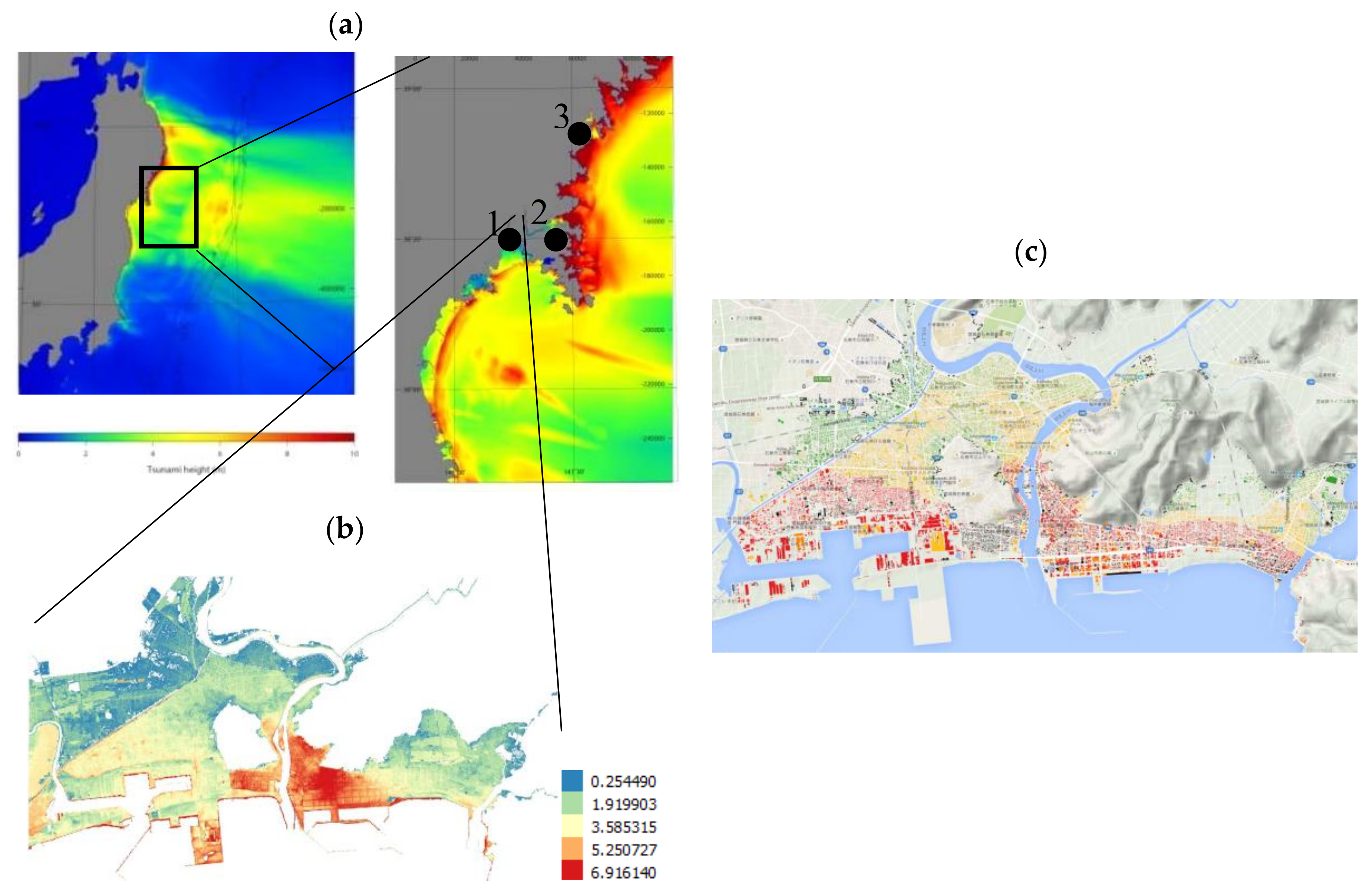
The numerical tsunami inundation model is presented in detail and validated by [19]. The tsunami source model used in this study is the time-dependent slip propagation model presented in [20]. The wave propagation and inundation calculation solves discretized non-linear shallow-water equations [15,21] over six computational domains in a nested grid system. The non-linear shallow-water equation includes the effects of flow resistance, which is parameterised using uniform value of the Manning’s roughness coefficient (n = 0.025). The example results shown in Figure 4 are the peak values for each grid square over the simulation period are the peak values for each grid square over the simulation period.
4. Application of Methodology to Case Study Data
4.1. Step 1: Exploratory Analysis of Debris-Induced Bias (Case Study)
A regular grid of 500 m is applied to each case study location (Figure 5). The total footprint area of all “washed away” (DS6) buildings is calculated for each grid square. If this area exceeds a threshold proportion of the total building footprint area for that grid all buildings of that grid square are designated as having been affected by debris. The levels of threshold proportions (i.e., washed away area/total area) are selected arbitrarily, and for the needs of this study three levels are tested: 20%, 35% and 50%.
Table 2 shows the number of buildings in the grid squares deemed to be affected by debris. As expected, the lowest collapse area threshold (of 20%) leads to the greatest number of buildings being removed from the dataset. Examining the damage states, inundation depths and forces experienced at building locations shows that buildings affected by debris generally fall into higher DS categories and at higher tsunami intensities.
Fragility functions are formed for all engineered buildings, and for those designated as affected or unaffected by debris, for the 20%, 35% and 50% collapse area thresholds. Reference [8] demonstrates that the optimal TIMs for this dataset are inundation depth and a measure of force, and so both of these TIMs are adopted here. Partially-ordered cumulative link models with a probit link function (model (2)) are formed on the logarithms of the selected TIMs, as this model is shown by [8] to fit this dataset well.
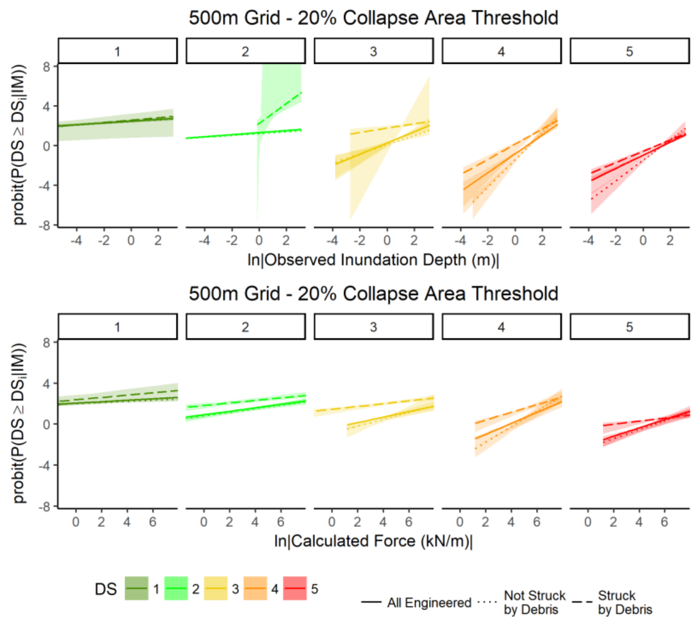
The fragility functions formed for all engineered buildings (i.e., the complete 4570-building dataset, ignoring debris) are considered as the base-case. It is seen that fragility functions for buildings with/without debris-impact deviate from the base-case, with the size of that deviation increasing with lower threshold values (i.e., the greatest deviations are seen for functions formed on data for the 20% collapse area threshold). Figure 6 therefore compares fragility functions formed for all engineered buildings, and for those designated as affected or unaffected by debris, for the 20% collapse area threshold (visible trends are similar for the 50% and 35% thresholds). Note that Figure 6 is plotted in link-space such that the x- and y-axes are transformed (indicated in the axis titles) so that the fragility functions appear as straight lines (Equation (2)), allowing trends to be more easily seen.
Intuitively, lower damage exceedance probabilities are expected in the absence of debris-related damage (i.e., a given flow depth may be deemed as more likely to cause damage if debris is also present in the flow). Therefore, taking fragility functions formed for all engineered buildings as the base-case (solid line, Figure 6), then the expected trend in Figure 6 is that damage exceedance probabilities should be higher for functions formed on debris-impacted buildings (dashed line, Figure 6) and lower for functions formed on buildings not struck by debris (dotted line, Figure 6). This expected trend is indeed shown in Figure 6, with some exceptions. For depth, the exceptions lie at lower depths for DS3 and very high depths at DS4 and DS5, where the damage exceedance probabilities for buildings not struck by debris are greater than the base case. For force, the exceptions lie at high force levels for DS4 and very high force levels for DS5 where the damage exceedance probabilities for buildings not struck and struck by debris are greater and lower than the base case respectively. Consider that for the expectation to be upheld at all TIM values then the curves must be perfectly parallel, but the methodology used does not prescribe this, meaning that they will inevitably cross at some point. It may therefore be that these highlighted, counterintuitive instances are due to a lack of data at these TIM ranges to constrain the functions. This crossing of the curves can be prevented by including the debris term within the model (and omitting an interaction term, so that the curves remain parallel), as will be conducted in Step 2 below.
It can be seen in Figure 6 that the confidence intervals at lower damage states are wider for buildings struck by debris, which reflects the fact that there are not many debris-affected buildings at these lower damage states. I.e., Buildings in the vicinity of other washed away buildings, DS6, are likely to have experienced higher damage states themselves. This is intuitive, as it would be expected that debris-affected buildings should experience greater damage. It can also be seen that confidence intervals are narrower for force (Figure 6, bottom) compared to depth (Figure 6, top), which might be considered to indicate reduced uncertainty when considering force as a TIM.
Therefore, the exploratory analysis presented in Figure 6 demonstrates that the consideration of debris effects has a sizeable impact on the resulting fragility functions, and so this impact should be quantified in Step 2 of the methodology, below.
4.2. Step 2: Quantifying the Effect of Debris in Fragility Function Derivation (Case Study)
The effect of debris on fragility function derivation is quantified by the addition of a debris term in the fragility functions, and the testing of this term to ascertain whether it leads to a statistically significant better fit to the data. A single model is formed which considers all engineered buildings and the significance of each parameter is determined by their p-values (Table 3). A likelihood ratio test is carried out to determine whether there is a significant increase in model accuracy with the addition of the debris terms (Table 4).
The p-values in Table 3 show that all debris parameters are significant and that the null hypothesis (that debris has no influence on damage state) can be rejected with the exception of the debris and debris interaction terms for DS1 (β2,DS1 and β3,DS1). The LRT results in Table 4 give p-values << 0.001 showing that the reduction in the residual sum of squares for the more complex model is statistically significant, so inclusion of debris in the fragility function formulation improves the performance of fragility functions.
4.3. Step 3: Quantification of Impact on Financial Loss Estimation (Case Study)
Section 4.2 demonstrates that debris effects influence fragility function derivation. However, the question remains as to what impact this might have on the estimation of expected loss (E[L]) derived from those fragility functions. Equation (6) shows that accurate calculation of E[L] requires information on the value of the property and on the expected MDR for each damage state. The accurate definition of property value and expected MDR requires financial data which is beyond the scope of this paper. Hence, an approximate comparison of representative calculated losses is presented here to illustrate the impact that debris-effects can potentially have on loss forecasting.
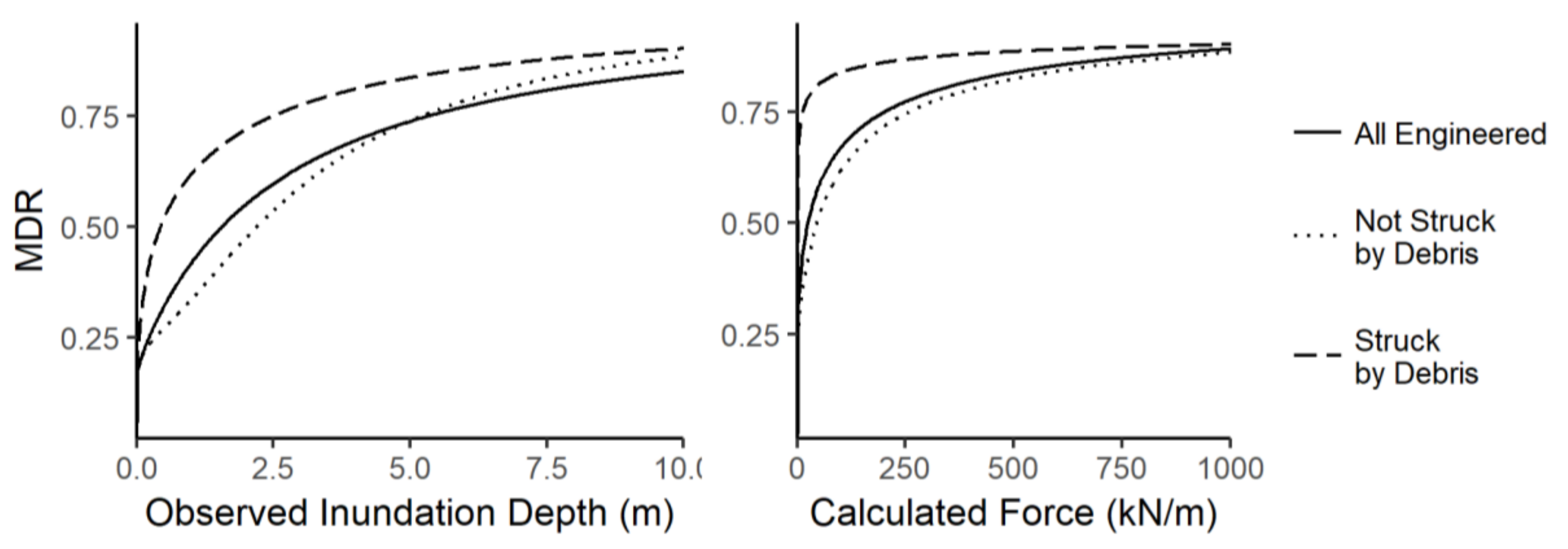
Preliminary vulnerability functions according to models (1) and (4) (considering only tsunami intensity, and incorporating debris, respectively) are shown in Figure 7. As per [22,23,24] and [25], MDRs of 0, 5, 20, 40, 60, and 100% are assumed for DS0, DS1, DS2, DS3, DS4, and DS5, respectively. The buildings considered for the loss estimation are the same engineered structures (presented in Section 2.1) used for the fragility derivation. The inundation scenario considered is the same 2011 Tsunami inundation presented in Section 3.2. In the absence of more recent and site-specific financial data a mean unit construction cost of 1600$/m2 is assumed as per [22,24,25]. The total construction cost for each building is then calculated by multiplying the unit construction cost by the footprint area and the number of stories. The total economic losses (the sums of expected loss for all the buildings in the dataset) are compared in Table 5.
Figure 7 shows that, as expected, the MDR for buildings which are not struck by debris are lower than those struck by debris, and generally lower than that when ignoring the effect of debris (except at higher inundation depths, the reason for which should be investigated in future studies). Table 5 shows that considering the effect of debris lowers the loss-estimate by between 1–1.5%, amounting to approximately 100$M–150$M in this particular scenario.
It is highlighted that the vulnerability functions cross at high values of inundation depth because of a lack of data with which to constrain the curves for this TIM range. This could be treated by removing the debris interaction term (β3 in Equation (3), so constraining the curves to be parallel.
Given a paucity of publicly available financial data, it is not possible to compare these results with observed losses during the 2011 Japan Tsunami, but this illustrative example serves to demonstrate that ignoring debris (or assuming that it is implicitly captured in the modelled inundation TIM), may lead to biases in loss estimation.
5. Conclusions
This paper has presented first steps towards quantifying the influence of debris-related effects on tsunami fragility and vulnerability assessment. A three-stage methodology is presented to conduct sensitivity analyses to determine the effect of debris impact on fragility and vulnerability curve derivation (so identifying bias in current studies), and to model more reliably the expected damage in areas with increased likelihood of debris. This methodology is demonstrated using a detailed damage dataset from the 2011 Great East Japan Earthquake and Tsunami.
The main results from this preliminary work are as follows:
- Debris-affected buildings mostly experienced higher TIM values and higher damage states (i.e., debris designation occurs in the vicinity of other ‘washed away’ buildings, which as more likely to occur in locations of high TIM values).
- The removal of buildings thought to be affected by debris resulted in changes to both the slope and intercept of the fragility functions. This indicates that the inclusion of debris-damaged buildings in the dataset does have an effect on fragility functions that may not be captured by purely flow regime-related TIMs.
- The difference between the intercept and slope for fluid-only and debris-influenced fragility functions can be quantified by inclusion of debris-indicator terms in the fragility functions.
- The influence of debris regression parameters on determining building damage is shown to be significant for all but the lowest damage state (“minor damage”), for the dataset used.
- More complex fragility functions which incorporate debris regression parameters are shown to have a statistically significant better fit to the observed damage data than models which omit debris information. This suggests that inclusion of debris information in fragility functions improves the accuracy of the model.
- Comparing simulated economic loss for estimates from vulnerability functions which do and do not incorporate a debris term suggests that biases in loss estimation may be introduced if not explicitly modelling debris.
Debris does not impact all areas in the same way and is expected to be more significant in areas of high urban density and high inundation, and so existing fragility studies may be biased if they do not account for debris. Further study is needed to more accurately quantify the effects of debris, however the research presented in this paper presents a step towards developing a methodology which is able to model more reliably the expected damage and losses in areas with increased likelihood of debris. This is of significant relevance for the engineering, disaster risk-reduction and insurance sectors, which all model predicted losses using vulnerability functions.
Acknowledgments
The time of Joshua Macabuag on the research for this paper was funded by EPSRC Engineering Doctorate Programme (EP/G037698/1) and the Willis Research Network. Joshua Macabuag’s travel to conduct this collaborative work was kindly funded by the Sasakawa Foundation and the Earthquake Engineering Field Investigation Team travel grant. The time of Dr Ioanna Ioannou for this research was funded by the EPSRC Challenging Risk grant (EP/K022377/1) and that of Professor Tiziana Rossetto was funded by the European Research Council under the auspices of the URBAN WAVES starting grant (336084). We would like to thank Richard Chandler of the Department of Statistical Science, UCL, for advising on the statistical analysis conducted in this study. Most significantly, we would like to acknowledge the many years of successful collaboration between EPICentre, UCL (UK) and IRIDeS, Tohoku University (Japan) which has made this work possible. Particular thanks is due to the following IRIDeS members: Anawat Suppasri, Daisuke Sugawara, Bruno Adriano, Fumihiko Imamura, Shunichi Koshimura.
Author Contributions
Tiziana Rossetto conceived the research question and advised on the paper, Joshua Macabuag wrote the majority of the paper, and Ioanna Ioannou contributed to and advised on the statistical analysis and the paper as a whole. Ian Eames provided initial guidance.
Conflicts of Interest
The authors declare no conflict of interest.
References
- Charvet, I.; Macabuag, J.; Rossetto, T. Estimating Tsunami-Induced Building Damage Through Fragility Functions: Critical Review and Research Needs. Front. Built Environ. 2017. [Google Scholar] [CrossRef]
- Tarbotton, C.; Dall’Osso, F.; Dominey-Howes, D.; Goff, J. The use of empirical vulnerability functions to assess the response of buildings to tsunami impact: Comparative review and summary of best practice. Earth Sci. Rev. 2015, 142, 120–134. [Google Scholar] [CrossRef]
- Suppasri, A.; Charvet, I.; Imai, K.; Imamura, F. Fragility curves based on data from the 2011 Great East Japan tsunami in Ishinomaki city with discussion of parameters influencing building damage. Earthq. Spectra 2014, 31, 841–868. [Google Scholar] [CrossRef]
- Earthquake Engineering Field Investigation Team (EEFIT). Field Report: Earthquake and Tsunami of 11th March 2011. Available online: https://www.istructe.org/getattachment/resources-centre/technical-topic-areas/eefit/eefit-reports/EEFIT-Japan-Recovery-Return-Mission-2013-Report-(1).pdf.aspx (accessed on 17 March 2018).
- Koshimura, S.; Namegaya, Y.; Yanagisawa, H. Tsunami Fragility — A New Measure to Identify Tsunami Damage. J. Disaster Res. 2009, 4, 479–488. [Google Scholar] [CrossRef]
- Charvet, I.; Suppasri, A.; Imamura, F. Empirical fragility analysis of building damage caused by the 2011 Great East Japan tsunami in Ishinomaki city using ordinal regression, and influence of key geographical features. Stoch. Environ. Res. Risk Assess. 2014, 28, 1853–1867. [Google Scholar] [CrossRef]
- Tanaka, N.; Onai, A.; Kondo, K. Fragility curve of region of wooden building washout due to tsunami based on hydrodynamic characteristics of the Great East Japan Tsunami. Ocean Eng. 2015, 71. [Google Scholar] [CrossRef]
- Macabuag, J.; Rossetto, T.; Ioannou, I.; Suppasri, A.; Sugawara, D.; Adriano, B.; Imamura, F.; Eames, I.; Koshimura, S. A proposed methodology for deriving tsunami fragility functions for buildings using optimum intensity measures. Nat. Hazards 2016, 84, 1257–1285. [Google Scholar] [CrossRef]
- Charvet, I.; Suppasri, A.; Kimura, H.; Sugawara, D.; Imamura, F. Fragility estimations for Kesennuma City following the 2011 Great East Japan Tsunami based on maximum flow depths, velocities and debris impact, with evaluation of the ordinal model’s predictive accuracy. Nat. Hazards 2015, 79, 2073–2099. [Google Scholar] [CrossRef]
- Macabuag, J.; Rossetto, T.; Ioannou, I. Investigation of the Effect of Debris-Induced Damage for Constructing Tsunami Fragility Curves for Buildings. In Proceedings of the 1st International Conference on Natural Hazards & Infrastructure, Crete, Greece, 28–30 June 2016. [Google Scholar]
- Rossetto, T.; Ioannou, I.; Grant, D.N.; Maqsood, T. Guidelines for Empirical Vulnerability Assessment. Available online: https://www.researchgate.net/profile/Tiziana_Rossetto/publication/265300146_Guidelines_for_empirical_vulnerability_assessment/links/561e71f608ae50795afefafc/Guidelines-for-empirical-vulnerability-assessment.pdf 2014 (accessed on 14 March 2018).
- Charvet, I.; Ioannou, I.; Rossetto, T.; Suppasri, A.; Imamura, F. Empirical fragility assessment of buildings affected by the 2011 Great East Japan tsunami using improved statistical models. Nat. Hazards 2014, 73, 951–973. [Google Scholar] [CrossRef]
- Muhari, A.; Charvet, I.; Tsuyoshi, F.; Suppasri, A.; Imamura, F. Assessment of tsunami hazards in ports and their impact on marine vessels derived from tsunami models and the observed damage data. Nat. Hazards 2015, 78, 1309–1328. [Google Scholar] [CrossRef]
- Japan Cabinet Office. Residential Disaster Damage Accreditation Criteria Operational Guideline. Available online: http://www.bousai.go.jp/taisaku/unyou.html (accessed on 17 March 2018).
- Suppasri, A.; Mas, E.; Koshimura, S.; Imai, K.; Harada, K.; Imamura, F. Developing Tsunami Fragility Curves From the Surveyed Data of the 2011 Great East Japan Tsunami in Sendai and Ishinomaki Plains. Coast. Eng. J. 2012, 54. [Google Scholar] [CrossRef]
- Suppasri, A.; Mas, E.; Charvet, I.; Gunasekera, R.; Imai, K.; Fukutani, Y.; Abe, Y.; Imamura, F. Building damage characteristics based on surveyed data and fragility curves of the 2011 Great East Japan tsunami. Nat. Hazards 2013, 66, 319–341. [Google Scholar] [CrossRef]
- Qi, Z.X.; Eames, I.; Johnson, E.R. Force acting on a square cylinder fixed in a free-surface channel flow. J. Fluid Mech. 2014, 756, 716–727. [Google Scholar] [CrossRef]
- Foster, A.S.J.; Rossetto, T.; Allsop, W. An experimentally validated approach for evaluating tsunami inundation forces on rectangular buildings. Coast. Eng. 2017, 128, 44–57. [Google Scholar] [CrossRef]
- Adriano, B.; Koshimura, S.; Hayashi, S.; Gokon, H.; Mas, E. Understanding the extreme tsunami inundation in onagawa town by the 2011 tohoku earthquake, its effects in urban structures and coastal facilities. Coast. Eng. J. 2016, 58. [Google Scholar] [CrossRef]
- Satake, K.; Fujii, Y.; Harada, T.; Namegaya, Y. Time and Space Distribution of Coseismic Slip of the 2011 Tohoku Earthquake as Inferred from Tsunami Waveform Data. Bull. Seismol. Soc. Am. 2013, 103, 1473–1492. [Google Scholar] [CrossRef]
- Imamura, F.; Gica, E.; Takahashi, T.; Shuto, N. Numerical Simulation of the 1992 Flores Tsunami: Interpretation of Tsunami Phenomena in Northeastern Flores Island and Damage at Babi Island. Pure Appl. Geophys. 1995, 144, 555–568. [Google Scholar] [CrossRef]
- De Risi, R.; Goda, K.; Mori, N.; Yasuda, T. Bayesian tsunami fragility modeling considering input data uncertainty. Stoch. Environ. Res. Risk Assess. 2017, 31, 1253–1269. [Google Scholar] [CrossRef]
- Ministry of Land, Infrastructure and Transport (MLIT). Survey of Tsunami Damage Conditions; MLIT: Tokyo, Japan, 2014.
- Ministry of Land, Infrastructure and Transport (MLIT). National Statistics; MLIT: Tokyo, Japan, 2015.
- Construction Research Institute (CRI). Japan Building Cost Information; CRI: Tokyo, Japan, 2011; p. 547. [Google Scholar]
Figure 1.
Fragility functions for ria (mountainous) coast (a) and coastal plains (b), but both from the same city of Ishinomaki, Japan [3]. This suggests that using only one Tsunami Intensity Measure (TIM), inundation depth, is insufficient to capture the damage potential of the flow.
Figure 1.
Fragility functions for ria (mountainous) coast (a) and coastal plains (b), but both from the same city of Ishinomaki, Japan [3]. This suggests that using only one Tsunami Intensity Measure (TIM), inundation depth, is insufficient to capture the damage potential of the flow.

Figure 2.
Evidence of debris effects on buildings, from the 2011 Japan Tsunami. (a) Likely large debris impact on the top floor of an overturned Reinforced Concrete-framed building; (b) Openings dammed by debris. (Photos: [4]).
Figure 2.
Evidence of debris effects on buildings, from the 2011 Japan Tsunami. (a) Likely large debris impact on the top floor of an overturned Reinforced Concrete-framed building; (b) Openings dammed by debris. (Photos: [4]).
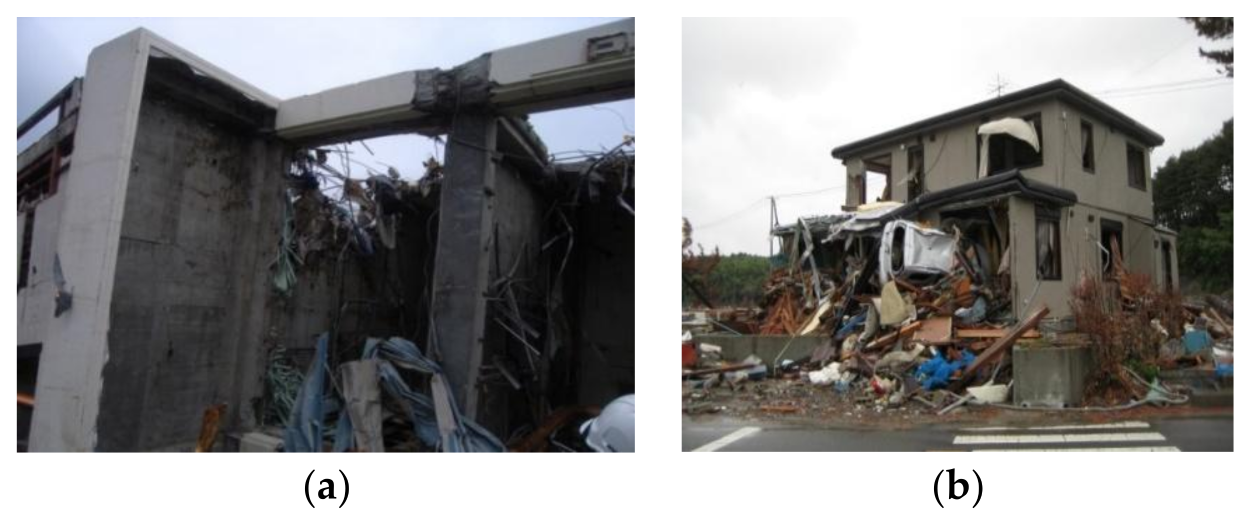
Figure 3.
Flow chart showing the 3-step methodology presented in this paper, to quantify the effect that debris-induced damage has on fragility and vulnerability function derivation, and subsequent loss estimates.
Figure 3.
Flow chart showing the 3-step methodology presented in this paper, to quantify the effect that debris-induced damage has on fragility and vulnerability function derivation, and subsequent loss estimates.

Figure 4.
Inundation and damage data referring to the 2011 Japan Tsunami. (a) Wave propagation results, with case-study locations indicated: 1 = Ishinomaki, 2 = Onagawa, 3 = Kesennuma. (b) Inundation simulation results for Ishinomaki (c) Building damage data with buildings coloured from green (damage state (DS)1) to red (DS5) with black indicating DS6.

Figure 5.
500 m grid used for debris analysis overlaid on case-study location Ishinomaki.
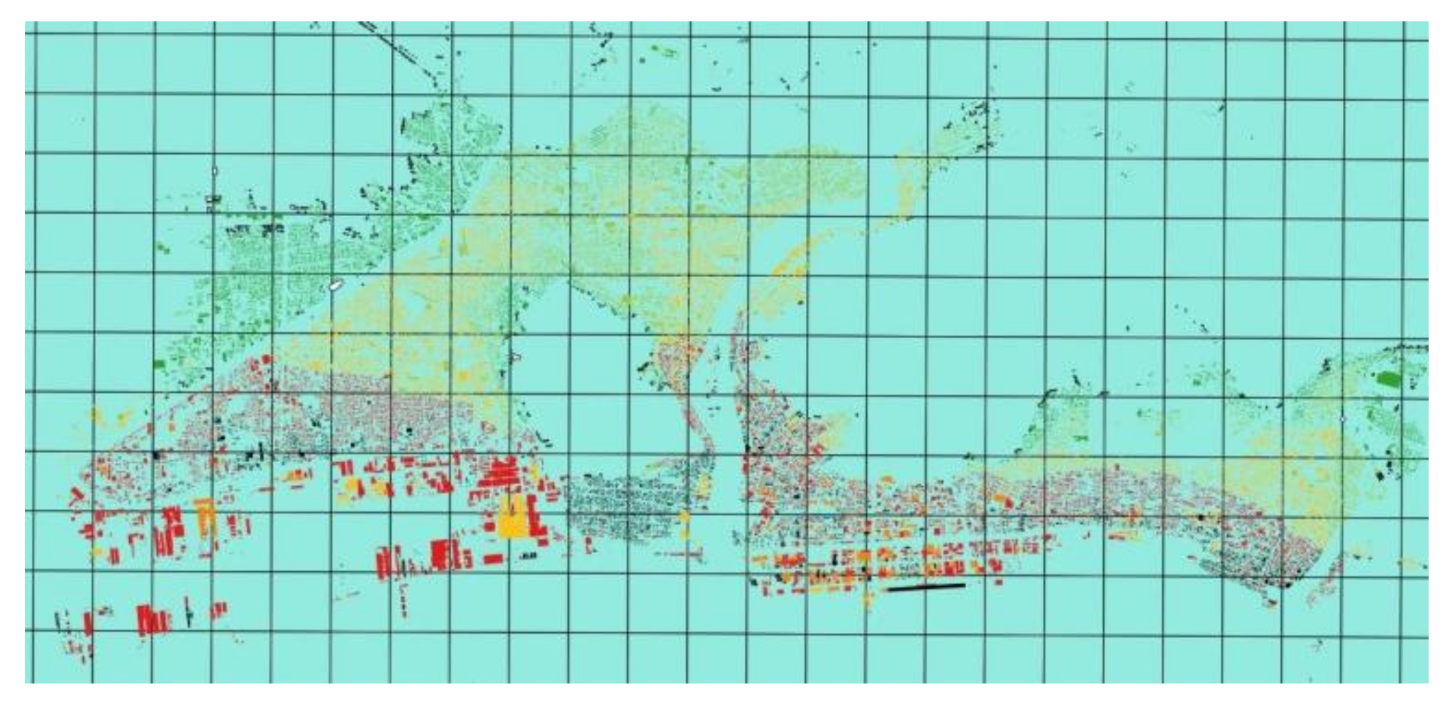
Figure 6.
Fragility functions for observed inundation depth (top) and simulated force (bottom) for fragility functions derived for all engineered buildings (solid line, with 95% bootstrap confidence intervals) and buildings which are/are not deemed to be affected by debris (for the 20% collapse area threshold). Some curve do not extend full the width of fig (e.g., DS2, TIM = h, struck by debris) as for some TIM values there is a cumulative probability of 0, such that probit(0) cannot be evaluated, and so the curve cannot be drawn for these TIM values.

Figure 7.
A comparison of vulnerability curves (mean damage ratio (MDR) vs. TIM), for all engineered buildings, those struck by debris and those not-struck by debris. Note that the curves pass through the origin, but increase instantly for all non-zero TIM values.
Figure 7.
A comparison of vulnerability curves (mean damage ratio (MDR) vs. TIM), for all engineered buildings, those struck by debris and those not-struck by debris. Note that the curves pass through the origin, but increase instantly for all non-zero TIM values.


Table 1.
Damage state definitions used by the Japanese Ministry of Land Infrastructure Tourism and Transport following the 2011 Great East Japan Earthquake and Tsunami. Descriptions from [14], usage descriptions are after [3].
| Damage State | Description | Use | Image | ||
|---|---|---|---|---|---|
| DS1 | Minor Damage | Inundation below ground floor. | Possible to use immediately after minor floor and wall cleanup. |  | |
| DS2 | Moderate Damage | The building is inundated less than 1m above the floor. | Possible to use after moderate repairs. |  | |
| DS3 | Major Damage | The building is inundated more than 1m above the floor (below the ceiling) | Possible to use after major repairs. |  | |
| DS4 | Complete Damage | The building is inundated above the ground floor level. | Major work is required for re-use of the building. |  | |
| DS5* | DS5 | Collapsed | The key structure is damaged, and difficult to repair to be used as it was before | Not repairable. |  |
| DS6 | Washed Away | The building is completely washed away except for the foundation | Not repairable. |  | |
Table 2.
Proportions of data designated as debris-affected under various collapse area thresholds.
| Threshold | Number of Buildings Designated as Affected by Debris | % of total Dataset (4570 Buildings) Affected by Debris |
|---|---|---|
| Base case (no buildings designated as having been affected by debris) | 0 | 0% |
| 50% of total grid building area | 588 | 13% |
| 35% of total grid building area | 778 | 17% |
| 20% of total grid building area | 1440 | 32% |
Table 3.
Regression parameters of model (4).
| Parameter | Parameter Description | Estimate | Std. Error | p | Significance 1 |
|---|---|---|---|---|---|
| β0 | 0|1.(Intercept) | 2.44 | 0.08 | 1.14 × 10−189 | *** |
| 1|2.(Intercept) | 1.20 | 0.03 | 5.01 × 10−294 | *** | |
| 2|3.(Intercept) | 0.11 | 0.03 | 2.89 × 10⁻⁵ | *** | |
| 3|4.(Intercept) | −1.41 | 0.05 | 1.31 × 10−190 | *** | |
| 4|5.(Intercept) | −1.45 | 0.05 | 2.93 × 10−163 | *** | |
| β1 | 0|1. ln|hobs j| | 0.08 | 0.01 | 2.69 × 10⁻³¹ | *** |
| 1|2. ln|hobs j| | 0.09 | 0.01 | 3.38 × 10−52 | *** | |
| 2|3. ln|hobs j| | 0.46 | 0.02 | 1.62 × 10−124 | *** | |
| 3|4. ln|hobs j| | 1.38 | 0.04 | 3.71 × 10−296 | *** | |
| 4|5. ln|hobs j| | 1.03 | 0.04 | 1.72 × 10−119 | *** | |
| β2 | 0|1. debrisj | 0.13 | 0.21 | 5.36 × 10⁻¹ | |
| 1|2. debrisj | 1.06 | 0.15 | 2.83 × 10⁻¹² | *** | |
| 2|3. debrisj | 1.67 | 0.10 | 1.57 × 10−64 | *** | |
| 3|4. debrisj | 1.58 | 0.12 | 2.90 × 10−38 | *** | |
| 4|5. debrisj | 0.89 | 0.11 | 2.37 × 10⁻¹⁵ | *** | |
| β3 | 0|1. ln|hobs j|. debrisj | 0.04 | 0.02 | 1.62 × 10⁻² | * |
| 1|2 . ln|hobs j|. debrisj | 0.91 | 0.23 | 6.58 × 10⁻⁵ | *** | |
| 2|3 . ln|hobs j|. debrisj | −0.24 | 0.04 | 1.74 × 10⁻⁸ | *** | |
| 3|4 . ln|hobs j|. debrisj | −0.61 | 0.08 | 1.44 × 10⁻¹⁵ | *** | |
| 4|5 . ln|hobs j|. debrisj | −0.46 | 0.07 | 6.89 × 10⁻¹¹ | *** |
1 Significance codes are: *** = p < 0.001, ** = p < 0.01, * = p < 0.05.
Table 4.
Likelihood ratio test results comparing models of increasing complexity based on observed inundation depth. Model numbers are defined in the text above. Equation (2) refers to model based on a single TIM, (3) includes a debris term, (4) includes a debris-TIM interaction term.
Table 4.
Likelihood ratio test results comparing models of increasing complexity based on observed inundation depth. Model numbers are defined in the text above. Equation (2) refers to model based on a single TIM, (3) includes a debris term, (4) includes a debris-TIM interaction term.
| Model | Number of Parameters | Akaike Information Criteria Statistic | Log-Likelihood | Pr (>Chisq) | |
|---|---|---|---|---|---|
| Random Component | Systematic Component | ||||
| Equation (1) | Equation (2) | 10 | 11,177 | −5578 | |
| Equation (3) | 15 | 10,547 | −5258 | <2.2 × 10⁻¹⁶ *** | |
| Equation (4) | 20 | 10,400 | −5180 | <2.2 × 10⁻¹⁶ *** | |
Table 5.
A comparison of indicative estimated losses due to building damage, for engineered buildings.
Table 5.
A comparison of indicative estimated losses due to building damage, for engineered buildings.
| Model Number | Model Description | Total Economic Loss (Calculated from Vulnerability Functions with the Following TIMs) | |
|---|---|---|---|
| Inundation Depth | Force | ||
| (1) | Considering a single TIM only | 4362$M | 4310$M |
| (4) | Considering Debris (and interaction) | 4231$M | 4175$M |
| Difference: | 1.2% | 1.4% | |
© 2018 by the authors. Licensee MDPI, Basel, Switzerland. This article is an open access article distributed under the terms and conditions of the Creative Commons Attribution (CC BY) license (http://creativecommons.org/licenses/by/4.0/).
Share and Cite
MDPI and ACS Style
Macabuag, J.; Rossetto, T.; Ioannou, I.; Eames, I. Investigation of the Effect of Debris-Induced Damage for Constructing Tsunami Fragility Curves for Buildings. Geosciences 2018, 8, 117. https://doi.org/10.3390/geosciences8040117
AMA Style
Macabuag J, Rossetto T, Ioannou I, Eames I. Investigation of the Effect of Debris-Induced Damage for Constructing Tsunami Fragility Curves for Buildings. Geosciences. 2018; 8(4):117. https://doi.org/10.3390/geosciences8040117
Chicago/Turabian StyleMacabuag, Joshua, Tiziana Rossetto, Ioanna Ioannou, and Ian Eames. 2018. "Investigation of the Effect of Debris-Induced Damage for Constructing Tsunami Fragility Curves for Buildings" Geosciences 8, no. 4: 117. https://doi.org/10.3390/geosciences8040117
Note that from the first issue of 2016, this journal uses article numbers instead of page numbers. See further details here.