Impact of Climate Change on Flood Frequency and Intensity in the Kabul River Basin
by
Muhammad Shahid Iqbal
1,*, 
Zakir Hussain Dahri
2,
Erik P Querner
3,
Asif Khan
4,5 and
Nynke Hofstra
1 1
Environmental Systems Analysis Group, Wageningen University and Research, 6708 PB Wageningen, The Netherlands
2
Water Systems and Global Change Group, Wageningen University and Research, 6708 PB Wageningen, The Netherlands
3
Querner Consult, 6709 DA, Wageningen, The Netherlands
4
Department of Civil Engineering, UET Peshawar, Jalozai Campus, Peshawar 25000, Pakistan
5
Centre for Water Informatics and Technology (WIT), LUMS, Lahore, Pakistan
*
Author to whom correspondence should be addressed.
Geosciences 2018, 8(4), 114; https://doi.org/10.3390/geosciences8040114
Submission received: 12 February 2018
/
Revised: 15 March 2018
/
Accepted: 15 March 2018
/
Published: 30 March 2018
(This article belongs to the Special Issue Hydrology in River Basins: Developments in Science and Application (HRBDSA))
Abstract
:Devastating floods adversely affect human life and infrastructure. Various regions of the Hindukush-Karakoram-Himalayas receive intense monsoon rainfall, which, together with snow and glacier melt, produce intense floods. The Kabul river basin originates from the Hindukush Mountains and is frequently hit by such floods. We analyses flood frequency and intensity in Kabul basin for a contemporary period (1981–2015) and two future periods (i.e., 2031–2050 and 2081–2100) using the RCP4.5 and RCP8.5 scenarios based on four bias-corrected downscaled climate models (INM-CM4, IPSL-CM5A, EC-EARTH, and MIROC5). Future floods are modelled with the SWAT hydrological model. The model results suggest an increasing trend due to an increasing precipitation and higher temperatures (based on all climate models except INM-CM4), which accelerates snow and glacier-melt. All of the scenario results show that the current flow with a 1 in 50 year return period is likely to occur more frequently (i.e., 1 in every 9–10 years and 2–3 years, respectively) during the near and far future periods. Such increases in intensity and frequency are likely to adversely affect downstream population and infrastructures. This, therefore, urges for appropriate early precautionary mitigation measures. This study can assist water managers and policy makers in their preparation to adequately plan for and manage flood protection. Its findings are also relevant for other basins in the Hindukush-Karakoram-Himalayas region.
1. Introduction
Recurring floods often pose devastating effects in terms of human sufferings and material losses. The Indus basin, originating from the Hindukush-Karakorum-Himalayan (HKH) region, is prone to such extreme flood hazards. The basin has been strongly hit by destructive floods during recent decades and this induced massive infrastructural, socio-economic, and environmental damages (see Figure S1). The cumulative estimated economic losses of more than US $45.607 billion are reported. Around 12,655 people lost their lives and nearly 200,000 villages were damaged or destroyed due to these floods in the past 80 years. The most devastating flood in 2010 spread over an area of about 160,000 km−2 across 82 districts affected over 20 million people, including about 2000 deaths and 3000 injuries.
Kabul river, the largest tributary of the Indus river on its right side, originates in Afghanistan and brings frequent intensive flash floods in its low-land downstream areas, particularly when heavy monsoon rains are joined by snowmelt runoff during the summer months [1]. The most severely affected areas by the 2010 flood include the Peshawar, Charsadda, Mardan, Nowshera, Swabi, and Swat districts that are located in lower reaches of the Kabul river. All of these districts suffered from massive damages (see Table S1).
A warming climate and changes in precipitation patterns are expected to substantially influence river flows in the HKH region, including the Kabul basin [2]. The mean surface temperature increase in the HKH region towards 2100 is expected to be higher than the global mean surface temperature increase [3]. This temperature increase will probably cause considerable changes in the region’s weather patterns hydrological cycle. Relative to the 1961–1990 baseline period, the mean temperature during the near future (i.e., 2021–2050) period is projected to rise 2 °C, and an average change of 8% to 12% in annual precipitation is projected under the RCP4.5 [4]. The change in mean temperature and precipitation will probably become larger in the far future (i.e., 2081–2100), due to the increasing greenhouse gas concentrations [2,5]. Western low pressure weather systems, which generate most of the winter precipitation in the Hindukush and Karakorum regions, are expected to be accelerated by the changing climate [6,7]. This can maintain a positive snow/glacier mass balance. This positive mass balance coupled with the increasing summer temperatures and monsoon precipitation will not only intensify the snow/glacier melt, but also bring in extreme floods.
To better prepare for the recurring natural flood hazards and prevent financial losses and casualties, the possible future changes in flood frequency and the intensity in the Kabul river basin should be analysed. However, such analysis for this important river basin is still lacking. This study therefore determines the projected future climate change and assesses its impacts on river flows in the Kabul river basin. The study provides quantitative estimates of the projected changes in flood frequency and intensity for both the near future (i.e., 2031–2050) and far future (i.e., 2081–2100) periods relative to the contemporary period (i.e., 1981–2000). The results of this study will be vital to develop effective flood risk management plans and to design safeguarded hydraulic infrastructures along the Kabul River.
This paper is structured as follows. In Section 2, we describe the study area in more detail. Section 3 describes the data used and prepared for the analysis. Section 4 explains the approach used in the hydrological model, flood frequency analysis, and selection of climate models. Section 5 described the results followed by the discussion. Finally, the major findings are presented in the conclusion.
2. The Study Area
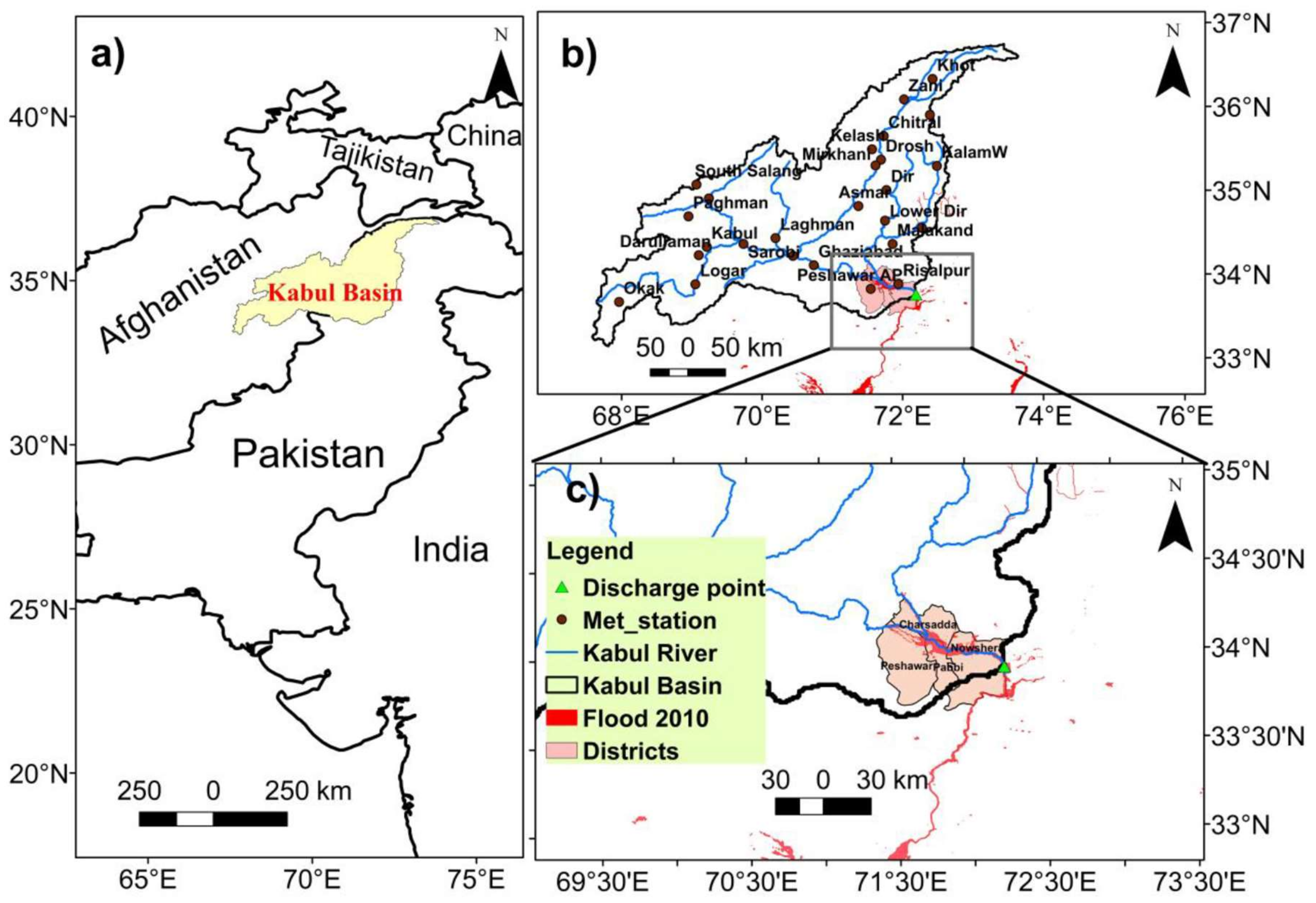
The Kabul River originates from the Sanglakh range of the Hindukush mountains in Afghanistan and sustains the livelihoods of millions of people in Afghanistan and Pakistan (Figure 1a). It contributes around 10% to 12% of the annual flows to the main Indus river system [8]. The total area of the Kabul basin is approximately 92,650 km2. Its main tributaries are the Salang, Panjshir, Nerkh, Maidan, Duranie, Kunar, Swat, Jindi, Barra, and Kalpani Rivers. The Kabul basin can be divided into three major sub-basins on the basis of flow generation: the upper Kabul, Panjshir, and lower Kabul. The upper Kabul basin generates 2.6% of the average annual flow of the basin, because this part of the basin receives less rainfall and there is no snowmelt contribution in its annual flow, Panjshir generates almost 15% of the annual flow, while the rest of the flow is generated by the lower parts of the Kabul River, including Chitral, Swat, Jindi, and Barra tributaries [9].
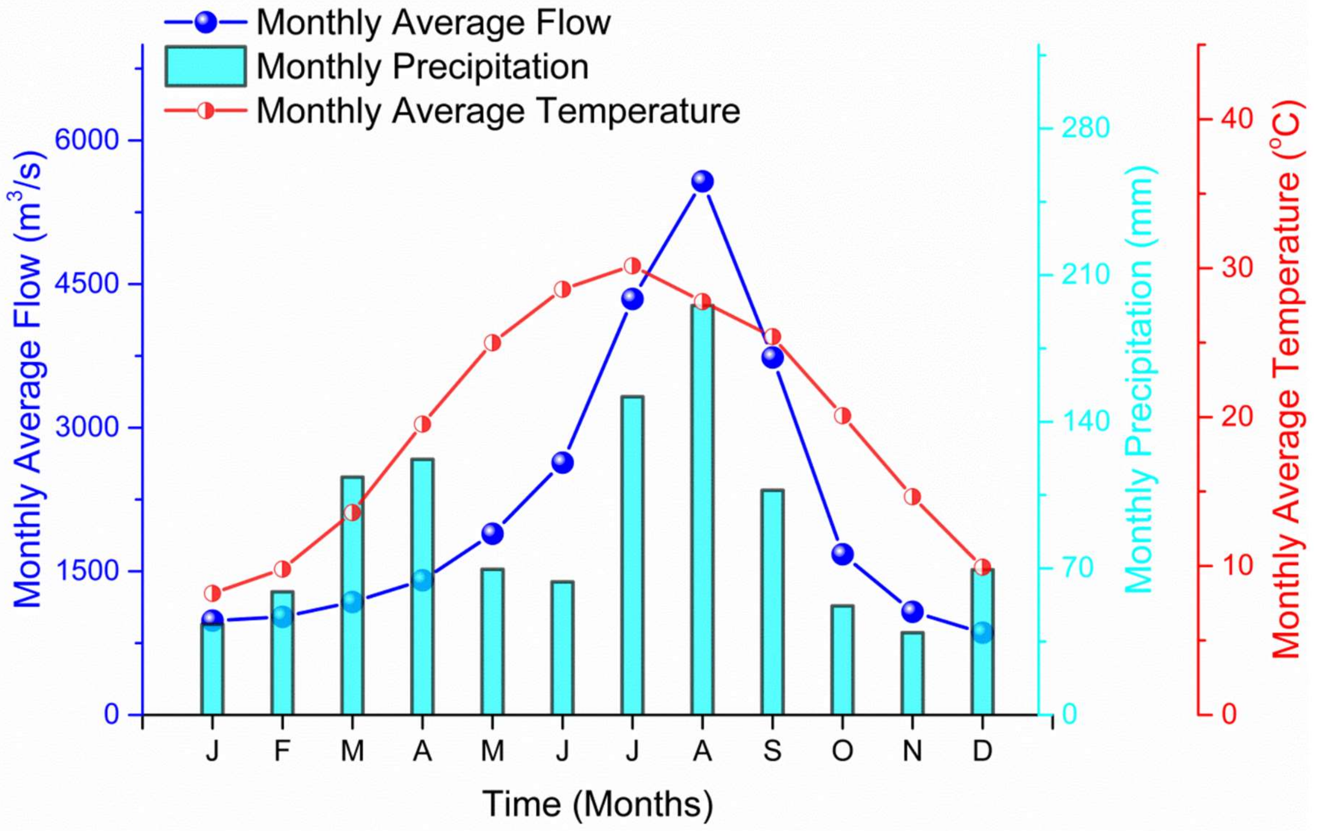
The basin’s average monthly temperature reaches its maximum in July, when snow and glacier-melt considerably contribute to river flows. Mean monthly precipitation encounters two peaks throughout a year: in April and August. The August peak precipitation predominantly stems from the Indian summer monsoon and is mainly experienced in the Chitral, Swat and extreme lower reaches of the Kabul River. The upper Kabul and Panjshir basins are mainly influenced by western disturbances (WDs) that originate from the Mediterranean Sea and receive peak precipitation during April. Chitral and Swat basins are also complemented with snow- and glacier-melt. These factors together cause the major floods along the Kabul River, particularly in low-land areas in the lower Kabul basin (Figure 1c). Mean monthly river flows that were observed at the Attock rim station (Figure 1b) indicates that about 80% of the annual flows occur during the April–September months with a peak in August (Figure 2).
Elevation of the basin ranges between 271 m and 7603 m, while its topography comprises high mountains with steep slopes (up to 10%) in the north and western part, and low slopes (up to 2%) and valleys in the lower basin (Figure S2a). Land use of the Kabul basin consists of agriculture (29.4%), pasture land (26.1%), urban area (19.7%), barren area (9.4%), water bodies (14.6%), and forest (0.6%) (Figure S2b). The predominant soil texture is loam to clay-loam textured (85%) and additionally 12% of the area’s soil is silty-clay, while only 3% is clay [10] (Figure S2c).
3. Data
3.1. Topographic, Soil and Land-Cover Data
Delineation of the Kabul basin was carried out using a 90 m resolution Digital Elevation Model (Figure S2) from the Shuttle Radar Topography Mission, acquired in January 2016 from the website (http://srtm.csi.cgiar.org). The Harmonized World Soil Database (available from http://webarchive.iiasa.ac.at/Research/LUC/External-World-soil-database) and European Space Agency’s land cover data for 2009 [11] (available from http://due.esrin.esa.int/page_globcover.php) were employed.
3.2. Historic Hydro-Climatic Data
The Pakistan climatic data includes, daily precipitation, daily min, max temperature, wind speed, relative humidity, and solar radiation for thirty-five years (1981–2015) was acquired from the Pakistan Meteorological Department, while the Afghanistan data was digitized/extracted from the country’s meteorological reports that were provided in shape of hard copies by the Afghanistan Meteorological Department (available at http://afghanag.ucdavis.edu/natural-resource-management/weather). Meteorological stations (either at the periphery or within the Kabul basin) in both countries were selected and used (see Figure 1b). Data from the selected meteorological stations were used to prepare the necessary weather input files for the SWAT model. Daily measured discharge data at the Attock rim station from January 1981 to December 2015 were acquired from the Water and Power Development Authority (WAPDA) of Pakistan. These observed flow data are used to analyse the flood frequency and calibration and validation of the SWAT model.
3.3. Future Climatic Data
3.3.1. GCM and Scenario Selection
General Circulation Models (GCMs) are used to simulate the global climate at different spatial resolutions (~100 km2 to ~250 km2) and to provide future climate change projections till 2100. GCMs are not preferred if RCMs datasets based on best available GCMs are available. Unfortunately, limited datasets are available for the study area, particularly RCMs data based on best available GCMs. In such conditions, the only way of climate change impact assessment is use of best available GCMs concomitant with robust bias-correction method. Extreme caution has been taken into account in the selection of GCMs and bias-correction method. The present-day cutting edge GCMs were prepared by the 5th Coupled Model Intercomparison Project CMIP5 [12]. The CMIP5’s data were the basis of the Fifth Assessment Report by the Intergovernmental Panel on Climate Change (IPCC). Over 61 publically available GCMs provide future climate data. However, most of these GCMs underestimate the monsoon precipitation in the HKH region and are not truly representative of this region [13]. Therefore, they cannot be directly used for the projection of extreme events (floods) [14]. A recent study by Lutz et al. [15] evaluated 94 GCM runs for RCP4.5 and 69 GCM runs for RCP8.5 for the HKH region using an advanced envelop-based selection approach that is integrated with the past performance of the GCMs. They shortlisted a climate model based on the projected average annual changes in the mean temperature and precipitation sum for the 2071–2100 period over the 1971–2000 period. The shortlisted GCM runs are further refined based on the changes in extremes of precipitation and temperature. Finally, the remaining GCM runs are validated by comparing their performance to reproduce the historical climate from a reference product. Lutz et al. (2016b), based on the same advance-envelop based approach, later selected four GCMs for the Upper Indus basin including the area under this study. We relied on Lutz et al. (2016b) and used the GCM runs that they selected for the upper Indus basin. We selected three GCMs that best represent the extremes of floods and droughts. The extreme of drought is represented by two possible dry-cold and dry-warm scenarios, while extreme floods are best represented by wet-warm scenario. The fourth GCM is selected on the basis of average conditions. The selected four GCMs are INM_CM4_r1i1p1 (Institute for Numerical Mathematics) for the dry-cold scenario, IPSL-CM5A-LR_r3i1p1 (Institute Pierre-Simon Laplace) for dry-warm scenario, MIROC5_r3i1p1 (Japanese Atmosphere and Ocean Research Institute, National Institute for Environmental Studies and Japan Agency for marine-earth Science and Technology) for wet-warm scenario, and EC-EARTH_r12i1p1 (EC-EARTH consortium) for the average scenario.
Climate change is expected to substantially alter the hydrological cycle, although projections of flow variations probably contain large uncertainties [16]. Due to such future climate uncertainties, researchers generally use different scenarios that indicate how future climate may change under specific assumptions. IPCC’s Fifth Assessment Report provides four Representative Concentration Pathways (RCPs) for climate-change projections and modelling. However, in our current study, climatic data for two representative concentration pathways (RCPs) were selected and used: RCP4.5 represents a medium concentration stabilization scenario in which greenhouse gas emissions peak around 2040 and then decline and RCP8.5 depicts a very high baseline scenario where emissions continue to rise throughout this century [17]. The CMIP5 daily climatic data for the four GCMs both RCP scenarios were downloaded from the Earth System Grid Federation Portal (http://cmip-pcmdi.llnl.gov/cmip5/; https://esgf-data.dkrz.de/search/cmip5/) to be used in our analysis.
3.3.2. Bias Correction, Downscaling and Grid Cell Selection
The evident inconsistencies in the spatial resolutions of GCMs can be corrected by different downscaling methods. This is necessary when climate models are used to drive hydrological and other models. Many downscaling methods are available to produce climatic data for climate impact models [18]. Downscaling can be divided in two main categories: dynamic [19] and statistical downscaling [20]. We used the statistical downscaling method explained by Liu et al. [21]. Its advantage is that it produces the data for a point rather than a grid and this point can then be used directly in a hydrological model, such as SWAT, that depends on point data. Liu et al. (2015) use a delta method with a straight forward quantile to quantile correction.
This downscaling method requires selection of a grid cell for downscaling. The grid cell on top of the local meteorological station can be used or the grid cells surrounding different stations can be interpolated so that the meteorological station is centred in the grid [22]. The SWAT model automatically incorporates the virtual meteorological station and we assume that the virtual meteorological station is right on top of actual meteorological station. The difference between these two selection methods is small at the local scale [23]. So, we apply the single grid cell on top of the local meteorological station in the current study.
4. Methods
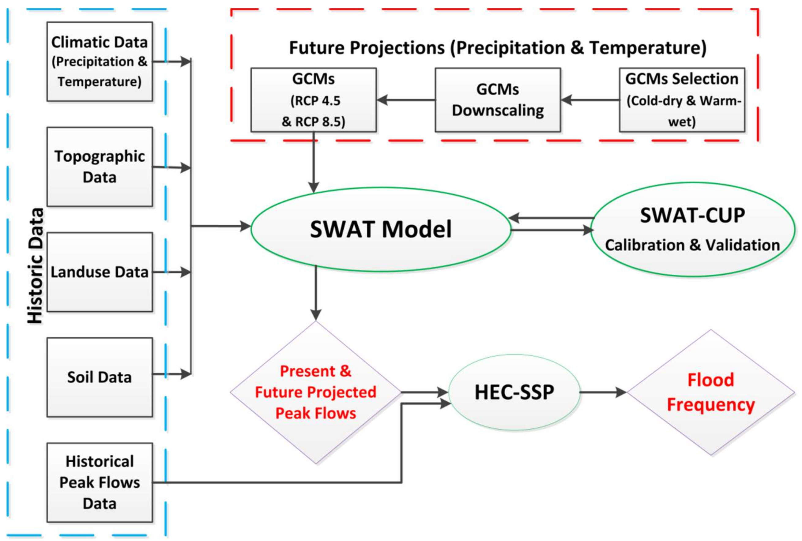
Flood frequencies are studied with historic annual flood data and with coupled hydrology (SWAT model) and flood frequency (HEC-SSP statistical software) for a reference period (1981–2000) and two future time periods (2031–2050 and 2081–2100). The future period of (2081–2100) has been selected, as base period is 1981-2000, therefore to predict 100 years change the time period has been selected and used. The methodology is summarized in Figure 3.
4.1. SWAT Model
The Soil and Water Assessment Tool (SWAT) is a river basin or watershed-scale model. It has been widely used for modelling watershed hydrology at continuous timescale. SWAT was developed to project the effects of water use, sediments and agricultural yields [24]. It is a physically based semi-distributed hydrologic model [24,25], which routes continuously on an hourly or daily time step. The SWAT model uses an ArcGIS interface for the definition of watershed hydrological features [24,26]. There are nine basic elements in the SWAT model: hydrology, weather, soil types, sediment yields, plant growth, nutrients loss, pesticides, bacterial load, and land-use management. The model subdivides the watershed into sub-basins based on a 90-m resolution digital elevation model. These sub-basins are further split up into hydrological response units (HRUs) that constitute land-use, soil, and slope features.
SWAT calculates potential evapotranspiration by applying the Penman-Monteith [27], Priestley-Taylor [28], or Hargreaves [29] parameterization depending on data availability. The Penman-Monteith method has been adopted in this study. The surface runoff from daily precipitation is computed with an altered curve- number method [30], which calculates the quantity of runoff based on data for the local land use and soil types. The land component ensures that the quantity of water, nutrients, sediments, bacteria, etc., are delivered to a primary channel in every individual sub-basin. All of the sub-basins are then directed through the main outlet of the basin.
The SWAT model requires hourly surface air temperature, while usually only daily maximum and minimum temperature are provided. Hourly surface air temperature is calculated as follows, assuming that the daily maximum temperature occurs at 15.00 o’clock and daily minimum temperature occurs at 03.00 o’clock [31]:
where Thr is the hourly surface air temperature (°C), hr is the hour, T’av is the average temperature on that day Tmx is the maximum temperature (°C), and Tmn is the daily minimum temperature (°C).
High altitudes of the upper part of the Kabul basin receive and store significant amounts of snowfall during winter and releases snow-melt during summer months. Therefore, the snowmelt factor has been included in the model calibration and validation. Equation (2) explains the snowmelt process in the model:
where SNOmlt is the amount of snow melt per day (mm water equivalent (w.e)), bmlt is the melt factor (mm day−1 °C−1 w.e), snocov is the fraction of the hydrological response unit’s area covered by snow, Tsnow is the temperature below which precipitation is considered as snow fall (°C), Tmx is the maximum temperature on a given day (°C), and Tmlt is the base temperature above which snow melt is allowed. Model has built-in property that it automatically incorporates the leap year in calculations. The factor bmlt can be estimated with the following equation:
where bmlt is the melt factor (mm day−1 °C−1 w.e), bmlt16 is the melt factor for 21 June (mm day−1 °C−1 w.e), bmlt12 is the melt factor for 21 December (mm day−1 °C−1 w.e), and dn is the day number of the year, where 1 is for 1 January and 365 is for 31st December [32].
4.2. Sensitivity Analysis, Calibration and Validation
Calibration is a crucial step in any hydrological modelling study to reduce the uncertainty in the modelled discharge [33], and validation is essential to trust the model’s performance [34]. For validation four years (2012–2015) of observed and simulated discharge data have been used. The calibration process generally requires a sensitivity analysis accompanied by manual or automatic calibration [35]. The sensitivity analysis was conducted using one-factor-at-a-time (OAT) sampling method that was proposed by Morris [36], which was applied in the Sequential Uncertainty Fitting SUFI-2 algorithm SWAT-CUP automatic sensitivity analysis tool [37] to see that changes in the model output represent to the parameter value changed. This method is robust and has been extensively used in modelling, but it demands long calculation times [38]. This sensitivity analysis also helped to evaluate how certain input variables influenced the model’s output. The analysis was done by changing individual variables by 10% of the initial value (keeping all of the other input variables constant) and examining the resulting effect on the predicted flow by the model. Ideally, the calibration process should use three to five years of data and constitutes a broad range of hydrological events [39]. Here, five years (2007–2011) of observational and simulated discharge data have been used for calibration.
Calibration and validation were carried out by comparing simulated and observed daily discharge records using common hydrological modelling statistical parameters: the coefficient of determination (R2), Nash-Sutcliffe Efficiency Index (NSE), and the percent bias (PBIAS). Generally, model simulations are called satisfactory if NSE > 0.50, R2 > 0.60 and PBIAS is approximately 25%. Negative values of PBIAS indicate that the model overestimates flow while the positive values of PBIAS indicate underestimated flow [40]. Similarly, Moriasi et al. [41] and Parajuli [42] categorized the model performance as excellent if (NSE > 0.90), very good (NSE > 0.75–0.89), good (NSE > 0.50–0.74), fair (NSE > 0.25–0.49), Poor (NSE > 0.00–0.24), and unsatisfactory if (NSE = 0.00).
4.3. The HEC-SSP Framework
Flood frequency Analysis (FFA) shows the characteristics of a basin and possible extreme flood events. In the present study the FFA was executed using HEC-SSP for the Kabul basin to identify the return period of extreme flood events in the Kabul River. Annual maximum (AM) discharges are the basis for the analysis, as is common practice [43]. HEC-SSP is a statistical software package, developed by the US Army Corps of Engineers (http://www.hec.usace.army.mil/software/hec-ssp). The most recent HEC-SSP version has built-in FFA-Bulletin-17B procedures that have been adopted for flow frequency analysis. The FFA-Bulletin-17B procedure produces a probability plot based on the following equation:
where m is the rank of annual maximum flows values with the largest flood equal to 1, n is the number of flood peaks in the data set, while A and B are the constants dependent on which equation is used during the flood frequency analysis procedure. In case of Weibull A and B equal 0, for Median A and B equal 0.3 and for the Hazen method A and B equal 0.5. To provide a conservative recurrence period, in the current study the Median probability plotting position factors (A and B equal 0.3) have been adopted [44].
5. Results and Discussion
5.1. Present Day Hydrological Modelling and Flood Frequency Analysis
The sensitivity analysis was carried out for 14 different SWAT variables for daily flow using the model sensitivity tool (Table S2). These variables were selected because they influenced the model’s output. (Table S2) shows the influence of the five most sensitive variables. The most sensitive variable is the curve number (CN2). A 10% increase in CN2 increased the flow by 20%. Other sensitive variables have less influence on the model’s outputs. The SWAT model was calibrated for these 14 sensitive variables. The SWAT model is sensitive to fourteen parameters for which it has been calibrated (see Table S2). Other studies [45,46,47,48] adjust the same model parameters. The model has been calibrated and validated for 2007–2011 and 2012–2015, respectively. The model performance was good as measured and simulated flows correlated well with R2 ranging between 0.84 and 0.77 for calibration and validation, respectively. The NSE was 0.77 for calibration and 0.72 for validation periods. Percent bias (PBIAS) values were 22.2 and 17.7 for calibration and validation, respectively (see Figure 4). Underestimation can be found for peaks, particularly during the calibration period. Underestimation in winter flows was observed. However, as low-flows are not the focus of the current study, therefore such underestimation can/is ignored in the current study. Such underestimation is common in hydrological modelling and could be due to flow recording-errors, biases in precipitation data and hydrological modelling uncertainties. However, the timing of the peaks is accurate for the calibration and validation periods and PBIAS is still within the appropriate range. This suggests that the current SWAT model calibration parameters can be rightfully used for future flow modelling and flood frequency analyses.
Observed and simulated flows are usually high during June to September every year. This is evident from both the calibration and validation time periods. The magnitude of peaks varies from year to year. In the calibration graph (see Figure 4 top), for example the peak starts in March followed by July each year and lasts till the end of July. Similarly, a similar peak is also observed in the validation graph (see Figure 4 bottom). This peak occurs from March till August but the intensity of flow differs much.
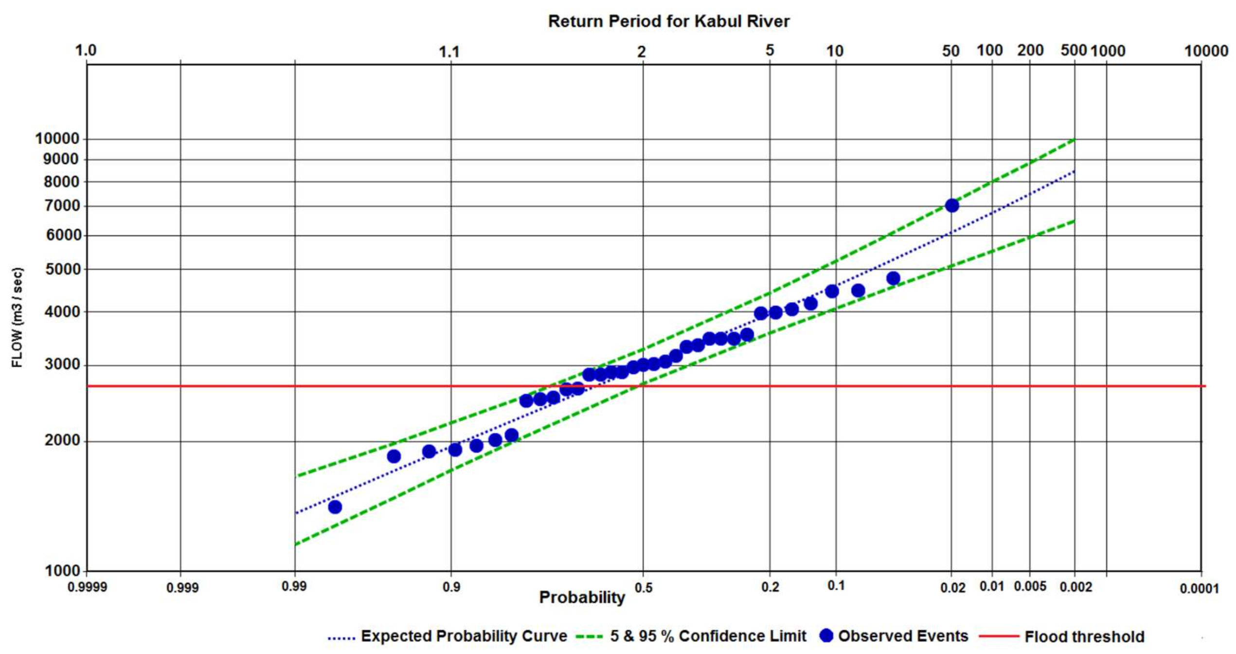
The HEC-SSP model was used to analyse flood return periods for the study area. In the Kabul River, especially in its low-land areas, flows that exceeds 2800 m3 s−1 are declared as floods [49]. The highest annual maximum peak flow was recorded in August 2010 (see Figure 5). This event has a probability of 0.02%, which equals 1 in 50 year event.
5.2. Future Discharge and Flood Frequency
Summer monsoon precipitation, snow, and glacier melt contribute to the peak flows of the Kabul River [50]. In this study, temperature and precipitation changes that are based on the four GCMs and two RCPs (RCP4.5 and RCP8.5) scenarios have been used to project changes in the Kabul river flows for the near future (2031–2050) and far future (2081–2100) periods. IPCC provides scenarios ranging from RCP2.6 to 8.5. As the current study deals with the extreme climate conditions (floods) therefore RCP4.5 and 8.5 have been selected, where RCP4.5 provides an average scenario, while RCP8.5 provides an extreme scenario, and is a common research practice by other well-known researchers. Mean monthly temperature is expected to rise towards the near and far future periods when compared to the contemporary reference period for both RCPs and all GCMs, except INM-CM4, which represents the cold-dry corner of our selected GCMs (see Figure 6a–d). Increased temperatures agree well with other studies [6,7,51]. Mean monthly precipitation also increases towards the near and far future periods for EC-EARTH and MIROC5 GCMs for both RCPs. However, precipitation declines in those periods for INM-CM4 GCM for both RCPs and a mixed response occurs for IPSL-CM5A (see Figure 6e–h). Variability is higher for precipitation than for temperature. Ahmad et al. [52] already observed that winter and autumn precipitation increased in the Swat River (a sub-basin of the Kabul River basin), based on their trend analysis of fifteen climate stations for the period 1961 to 2011. Ridley [6] and Wiltshire [7] also project increases in precipitation in the HKH region, including the Kabul River basin, in the mid to end of the 21st century.
Mean monthly modelled flows increases in the near and far future periods when compared to the historic flows for most GCMs and both scenarios. Only the INM-CM4 climate model shows a slight decline for both future periods and scenarios (see Figure 6i–l). In addition, seasonal flow variability could be expected in both future periods as compared to the reference period, although flows continue to peak in August for all GCMs and scenarios (see Figure 6i–l). Variation in flows could be driven by the following major factors. These are temperature driven variations in (i) precipitation, (ii) snow/glacier melt, (iii) clean ice exposure, (iv) debris-cover thickness, and (v) preceding winter snowfall. Therefore, to determine the main causes of the rise or decline in the Kabul basin’s river flows, all of these factors are evaluated and discussed below.
Our results suggest an increase in the near and far future flows as compared to the contemporary flows for both RCPs and all GCMs except for INM-CM4 (see Figure 6i–l), where flow temporal variations that are probably caused by temporal variations in precipitation (see Figure 6e–h). Ali et al. [53] and Rajbhandari et al. [54] concluded that flows in the nearby Upper Indus Basin indeed depend on the past precipitation variability. Thus, our results agree well with other studies.
In addition to precipitation, temperature variability also agrees well with the flows (see Figure 6a–d,i–l). Dey et al. [55] showed a strong relation between temperature and snow-melt in the Kabul basin and Archer [56] argued that summer river flows are mainly derived from the snow-melt of preceding winter snowfall in the Kunhar and Swat basins (sub-basins of the Kabul river basin). Archer’s (2003) argument is also complemented by other, more recent studies (see e.g., [2,57]). Therefore, an increase/decrease in temperature drives the increase/decrease in snow-melt during summer months. These arguments and results also agree well with the study’s result for the near and far future, where the rise/decline in temperature and flows are comparable.
The increased flows that we simulate are also supported by the literature. An increase in winter to early summer temperature probably reduces snowfall and accelerates snow-melt during the early summer months. Additionally, early seasonal snow-melt may also expose clean glacier ice, which can produce more melt during the summer months than the more airy snow. A decline in snow-cover has been observed by Savoskul and Smakhtin [58] in the Kabul basin between the periods 1960–1990 and 2000–2010. This decline in snow-cover expedited glacier-melt and resulted in a shrinking glacier length. Other studies e.g., [59,60,61,62] observed shrinkage in glacier length in the Hindukush region (including the Kabul basin). Early seasonal snow-melt and exposure of glacier ice, which resulted in a negative glacier mass balance (about −0.3 ± 0.1 m water equivalent per year based on 2003–2008 data analysis by Kääb et al. [63] and Kääb et al. [64], likely have supported part of the rising flows during peak summer months in the recent decades [58,65]. However, since the glacier length in the Kabul basin declined as per Randolph Glacier Inventory 5.0 data [66] to only 2.2% of the total basin area (approximately 2100 km2), its contribution to rising flows are probably small.
In contrast, Lutz et al. (2014) projected declines in the Kabul River flows by the end of 21st century. The main reasons for this contradiction with our results could be the use of different GCMs data, sub-optimal bias correction of GCM data, use of different hydrological models, and data from different time periods. The result by Lutz et al. [2] are part of study for much larger region, while for Kabul basin their results are not supported by literature. Therefore, based on the above results and discussion, an increase (decrease) in flows for the near and far future are caused by an increase (decrease) in precipitation, coupled to an increase (decrease) temperature. This enhances (suppresses) snow- and glacier-melt in the Kabul basin. Normally, the Kabul river flows are originated from snow-melt and rainfall runoff. In addition, the study region is extremely complex, as there would be rise in temperature together with increase in precipitation, therefore early snow-melt and rise in glacier-melt will encounter. Similarly increase in precipitation will enhance rainfall runoff.
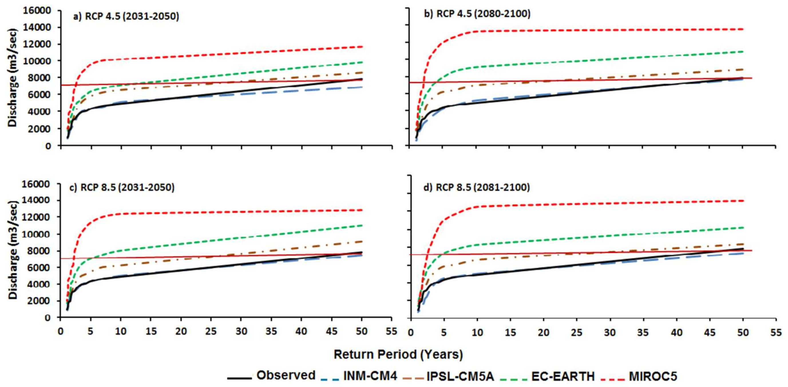
Increases in extreme precipitation events and a rise in temperature are the major sources of floods in the HKH region e.g., [1,67,68]. In our study, FFA has been carried out for the near future and far future peak flows (see Figure 7). FFA results show an increase in recurrence of peak flows for the near and far future and both RCP scenarios for all GCMs, except for INM-CM4, which show slight declines in the recurrence periods for both periods and RCPs. The result for MIROC5 provides the most extreme peak flow projection. For this model, the recurrence of the historic peak flow (i.e., the 2010 flood) is reduced from 1 in 50 years to 1 in less than 3 years for the near and far future periods and both RCPs. Projections for the other GCMs also suggest an intensification of future peak flows with a substantial reduction in the recurrence intervals during the near and far future periods.
FFA estimation is commonly used in hydrology and is usually performed to plan and design various hydraulic structures [69]. Dams and reservoirs could be built to protect the population and infrastructure from floods. In general, small dams are built to be strong enough to withstand a peak flood of a 100 year return period, while agricultural area protection infrastructure is designed for a 15–25 year return period flood [70]. When such structures are planned and built, the impacts of future climate change should be incorporated. Afghanistan plans to construct 13 dams for irrigation and energy production in the Kabul basin, upstream of the current study’s gauging station (FAO Aquastat, 2011). This new infrastructure should consider the changing return periods estimated in this study (see Table S3). That means that small dams should withstand flow up to approximately 15,000 m3/s m3 s-1. Our analysis thus provides insight into the boundary conditions of current and new infrastructure.
Our results can be used to prepare flood inundation plans and to study the vulnerability of various infrastructures and land and population at risk (see for example the inundation mapping by Tariq and van de Giessen [71]). The population in the most affected districts by the 2010 flood (shown in Figure 1c) is expected to become more vulnerable because of more frequent extreme flows and larger future population [35] in the flood plans. Our quantification of vulnerabilities assessment (e.g., Table S3) helps to prepare flood inundation maps, flood mitigation plans, and risk assessments.
6. Conclusions
Lower Kabul basin in Pakistan is often hit by intensive floods that cause devastating effects in terms of human suffering, economic losses, and infrastructural damages. The basin usually receives severe floods when high monsoon rainfall is joined by snow and glacier melt. The basin’s average monthly temperature reaches its maximum in July, while precipitation is bimodal, with peaks in April and August. April peaks result from the strong influence of western disturbances and August peaks predominantly stem from the Indian summer monsoon. The threshold level of floods is when river flows at Nowshera cross 2800 m3 s−1. The historical (1981–2015) flows reveal that this threshold level is attained more often than every second year. The exceptionally high and most devastating flood of 2010 was a one in 50 years event.
This study revealed substantial changes in hydro-climatology of the basin for both near and far futures. The GCMs MIROC5 and EC-EARTH project consistent increases in mean monthly temperature, precipitation, and river flows, while the INM-CM4 projects a slight decline for all three variables. IPSL-CM5A shows a slight increase in temperature and river flows, while for precipitation the response is mixed for RCP4.5 and increases for RCP8.5. These changes in river flow influence the flood frequency. The return periods are in most cases reduced. Depending on the scenario, GCM and period in the future, present day 1 in 50 year events could in the future occur from once in every three years to once in every 24 years.
Kabul River is an important part of the Indus river system. The low-altitude and densely populated areas in its downstream reaches are seriously threatened by frequent high-levels of floods. The biggest flood on record, in 2010, influenced a large area and killed over 2000 people. The results and analyses that are presented in our study indicate the hydrological implications of the projected climate changes in the basin until 2100. These changes have great practical implications for river discharge variation and occurrence of extreme events of floods and droughts. As the flow that caused the 2010 flood is expected to occur much more often in the future, climate proof flood protection measures are essential for the current and future water development and management plans in the Kabul River basin.
Supplementary Materials
The following are available online at https://www.mdpi.com/2076-3263/8/4/114/s1, Figure S1: Flood damages during 1950–2015 in the overall Indus Basin, Pakistan (FFC 2015), Figure S2: (a) Digital Elevation Model (resolution 90 m) ranges from 271 m to 7603 m (b) land-use classes, where FRSE = Forest, RNGE = Range Land/Pasture land, URHD = Urban area, WATR = Water bodies, BARR = Barren land, AGRC = Agricultural land close grown crops, and AGRL = General Agricultural land, all the land-use classes were taken from (Arnold et al. 2009) (c) soil types classification of the Kabul basin, Table S1: District-wise flood damages in 2010 in the lower Kabul basin in Pakistan (Khan and Mohmand, 2011), Table S2: Parameters selected and final calibrated values for SWAT-Model, Table-S3: Flow (m3/s) for the 5, 25, 50, 100, and 500 year return periods for RCP 4.5 and RCP 8.5 for all selected GCMs and observed annual maximum flow for the contemporary period (1981–2015), near (2031–2050) and far (2081–2100) future.
Acknowledgments
The authors would like to acknowledge Nuffic, Netherland Fellowship Program (NFP), and Government of the Netherlands for providing the PhD fellowship. The Pakistan Meteorological Department (Regional Meteorological Centre, Peshawar) and the Water and Power Development Authority Pakistan (WAPDA) are also acknowledged for providing hydro-meteorological data for the current study.
Conflicts of Interest
The authors declare no conflict of interest. The founding sponsors had no role in the design of the study; in the collection, analyses, or interpretation of data; in the writing of the manuscript, and in the decision to publish the results.
References
- Abbaspour, K. SWAT-CUP 2012: SWAT Calibration and Uncertainty Programs—A User Manual; EAWAG, Swiss Federal Institute of Aquatic Science and Technology: Zurich, Switzerland, 2012. [Google Scholar]
- Abbaspour, K.C.; Rouholahnejad, E.; Vaghefi, S.; Srinivasan, R.; Yang, H.; Kløve, B. A continental-scale hydrology and water quality model for Europe: Calibration and uncertainty of a high-resolution large-scale SWAT model. J. Hydrol. 2015, 524, 733–752. [Google Scholar] [CrossRef]
- Ahmad, I.; Tang, D.; Wang, T.; Wang, M.; Wagan, B. Precipitation trends over time using Mann-Kendall and Spearman’s rho tests in Swat River Basin, Pakistan. Adv. Meteorol. 2015, 2015, 431860. [Google Scholar] [CrossRef]
- Ali, A. Indus Basin Floods: Mechanisms, Impacts, and Management; Asian Development Bank: Mandaluyong, Philippines, 2013. [Google Scholar]
- Ali, S.; Li, D.; Congbin, F.; Khan, F. Twenty first century climatic and hydrological changes over Upper Indus Basin of Himalayan region of Pakistan. Environ. Res. Lett. 2015, 10. [Google Scholar] [CrossRef]
- Archer, D. Contrasting hydrological regimes in the upper Indus Basin. J. Hydrol. 2003, 274, 198–210. [Google Scholar] [CrossRef]
- Arendt, A.; Bliss, A.; Bolch, T.; Cogley, J.G.; Gardner, A.S.; Hagen, J.-O.; Hock, R.; Huss, M.; Kaser, G.; Kienholz, C.; et al. Randolph Glacier Inventory-A Dataset of Global Glacier Outlines: Version 5.0; Digital Media: Boulder, CO, USA, 2015; pp. 1–63. [Google Scholar]
- Arino, O.; Ramos, J.; Kalogirou, V.; Defourny, P.; Achard, F. GlobCover 2009. Press Release. 2010. Available online: http://due.esrin.esa.int/files/GLOBCOVER2009_Validation_Report_2.2.pdf (accessed on 23 July 2015).
- Arnold, J.G.; Srinivasan, R.; Muttiah, R.S.; Williams, J.R. Large area hydrologic modeling and assessment—Part I: Model development. J. Am. Water Resour. Assoc. 1998, 34, 73–89. [Google Scholar] [CrossRef]
- Bengston, L. Snowmelt-generated runoff in urban areas. In Proceedings of the Proceedings of the Second International Conference on Urban Storm Drainage, Urbana, IL, USA, 15–19 June 1981. [Google Scholar]
- Benham, B.L.; Baffaut, C.; Zeckoski, R.W.; Mankin, K.R.; Pachepsky, Y.A.; Sadeghi, A.M.; Brannan, K.M.; Soupir, M.L.; Habersack, M.J. Modeling bacteria fate and transport in watersheds to support TMDLs. Trans. ASABE 2006, 49, 987–1002. [Google Scholar] [CrossRef]
- Bolch, T.; Kulkarni, A.; Kääb, A.; Huggel, C.; Paul, F.; Cogley, J.G.; Frey, H.; Kargel, J.S.; Fujita, K.; Scheel, M.; et al. The state and fate of Himalayan glaciers. Science 2012, 336, 310–314. [Google Scholar] [CrossRef] [PubMed] [Green Version]
- Campbell, G.S. Soil Physics with BASIC: Transport Models for Soil-Plant Systems; Elsevier: Amsterdam, The Netherlands, 1985; Volume 14. [Google Scholar]
- Choi, I.; Munster, C.; Victor, D.; White, R.; Stewart, G.; Richards, C. Calibration and validation of the SWAT model on a field-scale watershed for turfgrass sod establishment. In Proceedings of the Watershed Management to Meet Water Quality Standards and Emerging TMDL (Total Maximum Daily Load), Atlanta, GA, USA, 5–9 March 2005. [Google Scholar]
- Dey, B.; Sharma, V.; Rango, A. A test of snowmelt-runoff model for a major river basin in western Himalayas. Hydrol. Res. 1989, 20, 167–178. [Google Scholar]
- Din, K.; Tariq, S.; Mahmood, A.; Rasul, G. Temperature and Precipitation: GLOF Triggering Indicators in Gilgit-Baltistan, Pakistan. Pak. J. Meteorol. 2014, 10, 192–201. [Google Scholar]
- Du, T.; Xiong, L.; Xu, C.-Y.; Gippel, C.J.; Guo, S.; Liu, P. Return period and risk analysis of nonstationary low-flow series under climate change. J. Hydrol. 2015, 527, 234–250. [Google Scholar] [CrossRef]
- Engel, B.; Storm, D.; White, M.; Arnold, J.; Arabi, M. A hydrologic/water quality model application 1. J. Am. Water Resour. Assoc. 2007, 43, 1223–1236. [Google Scholar] [CrossRef]
- FFC. Federal Flood Comission Annual Flood Report; FFC: Islamabad, Pakistan, 2015.
- Frischmann, P. Water Strategy Final Kabul River Basin Report; The World Bank: Washington, DC, USA, 2011. [Google Scholar]
- Gan, T.Y.; Dlamini, E.M.; Biftu, G.F. Effects of model complexity and structure, data quality, and objective functions on hydrologic modeling. J. Hydrol. 1997, 192, 81–103. [Google Scholar] [CrossRef]
- Gupta, H.V.; Sorooshian, S.; Yapo, P.O. Status of automatic calibration for hydrologic models: Comparison with multilevel expert calibration. J. Hydrol. Eng. 1999, 4, 135–143. [Google Scholar] [CrossRef]
- Hagemann, S.; Chen, C.; Clark, D.; Folwell, S.; Gosling, S.N.; Haddeland, I.; Hanasaki, N.; Heinke, J.; Ludwig, F.; Voss, F.; et al. Climate change impact on available water resources obtained using multiple global climate and hydrology models. Earth Syst. Dyn. 2013, 4, 129–144. [Google Scholar] [CrossRef]
- Hamby, D. A review of techniques for parameter sensitivity analysis of environmental models. Environ. Monit. Assess. 1994, 32, 135–154. [Google Scholar] [CrossRef] [PubMed]
- Hargreaves, G.H.; Samani, Z.A. Reference crop evapotranspiration from temperature. Appl. Eng. Agric. 1985, 1, 96–99. [Google Scholar] [CrossRef]
- Hartmann, H.; Buchanan, H. Trends in extreme precipitation events in the indus River Basin and flooding in Pakistan. Atmos. Ocean 2014, 52, 77–91. [Google Scholar] [CrossRef]
- Hawkins, E.; Osborne, T.M.; Ho, C.K.; Challinor, A.J. Calibration and bias correction of climate projections for crop modelling: An idealised case study over Europe. Agric. For. Meteorol. 2013, 170, 19–31. [Google Scholar] [CrossRef]
- IIASA; ISRIC; ISSCAS; FAO; JRC. Harmonized World Soil Database (Version 1.2). FAO, Rome, Italy and IIASA, Laxenburg, Austria. 2012. Available online: http://webarchive.iiasa.ac.at/Research/LUC/External-World-soil-database/HWSD_Documentation.pdf (accessed on 25 July 2015).
- Immerzeel, W.; Pellicciotti, F.; Bierkens, M. Rising river flows throughout the twenty-first century in two Himalayan glacierized watersheds. Nat. Geosci. 2013, 6, 742–745. [Google Scholar] [CrossRef]
- Inam, A.; Clift, P.D.; Giosan, L.; Tabrez, A.R.; Tahir, M.; Rabbani, M.M.; Danish, M. The geographic, geological and oceanographic setting of the Indus River. In Large Rivers: Geomorphology and Management; John Wiley & Sons, Ltd.: Hoboken, NJ, USA, 2007; pp. 333–345. [Google Scholar]
- IPCC. Climate Change 2013–The Physical Science Basis: Contribution of Working Group I to the Fifth Assessment Report of the Intergovernmental Panel on Climate Change; Qin, D., Stocker, T.S., Plattner, G.-K., Tignor, M., Allen, S.K., Boschung, J., Nauels, A., Xia, Y., Bex, V., Midgley, P.M., Eds.; Cambridge University Press: Cambridge, UK, 2014; pp. 1535–1542. [Google Scholar]
- IPCC. Summary for Policymakers. In Climate Change 2007: The Physical Science Basis. Contribution of Working Group I to the Fourth Assessment Report of the Intergovernmental Panel on Climate Change; Solomon, S., Qin, D., Manning, M., Chen, Z., Marquis, M., Averyt, K.B., Tignor, M., Miller, H.L., Eds.; Cambridge University Press: Cambridge, UK; New York, NY, USA, 2007. [Google Scholar]
- Kääb, A.; Berthier, E.; Nuth, C.; Gardelle, J.; Arnaud, Y. Contrasting patterns of early twenty-first-century glacier mass change in the Himalayas. Nature 2012, 488, 495–498. [Google Scholar] [CrossRef] [PubMed]
- Kääb, A.; Treichler, D.; Nuth, C.; Berthier, E. Brief Communication: Contending estimates of 2003–2008 glacier mass balance over the Pamir–Karakoram–Himalaya. Cryosphere 2015, 9, 557–564. [Google Scholar] [CrossRef]
- Kc, S.; Lutz, W. The human core of the shared socioeconomic pathways: Population scenarios by age, sex and level of education for all countries to 2100. Global Environ. Chang. 2017, 42, 181–192. [Google Scholar] [CrossRef] [PubMed] [Green Version]
- Lee, J.-Y.; Wang, B. Future change of global monsoon in the CMIP5. Clim. Dyn. 2014, 42, 101–119. [Google Scholar] [CrossRef]
- Leemans, R.; Cramer, W.P. The IIASA Database for Mean Monthly Values of Temperature, Precipitation, and Cloudiness on a Global Terrestrial Grid; International Institute for Applied Systems Analysis: Laxenburg, Austria, 1991. [Google Scholar]
- Leemans, R.; Monserud, R.; Solomon, A. A global biome model based on plant physiology and dominance, soil properties and climate. J. Biogeogr. 1992, 19, 11734. [Google Scholar]
- Liu, C.; Hofstra, N.; Leemans, R. Preparing suitable climate scenario data to assess impacts on local food safety. Food Res. Int. 2015, 68, 31–40. [Google Scholar] [CrossRef]
- Lutz, A.; Immerzeel, W.; Shrestha, A.; Bierkens, M. Consistent increase in High Asia’s runoff due to increasing glacier melt and precipitation. Nat. Clim. Chang. 2014, 4, 587–592. [Google Scholar] [CrossRef]
- Lutz, A.F.; ter Maat, H.W.; Biemans, H.; Shrestha, A.B.; Wester, P.; Immerzeel, W.W. Selecting representative climate models for climate change impact studies: An advanced envelope-based selection approach. Int. J. Climatol. 2016, 36, 3988–4005. [Google Scholar] [CrossRef]
- Madsen, H.; Pearson, C.P.; Rosbjerg, D. Comparison of annual maximum series and partial duration series methods for modeling extreme hydrologic events: 2. Regional modeling. Water Resour. Res. 1997, 33, 759–769. [Google Scholar] [CrossRef]
- Monteith, J. Evaporation and environment. Symp. Soc. Exp. Biol. 1965, 19, 205–234. [Google Scholar] [PubMed]
- Moriasi, D.N.; Arnold, J.G.; Van Liew, M.W.; Bingner, R.L.; Harmel, R.D.; Veith, T.L. Model evaluation guidelines for systematic quantification of accuracy in watershed simulations. Trans. ASABE 2007, 50, 885–900. [Google Scholar] [CrossRef]
- Morris, M.D. Factorial sampling plans for preliminary computational experiments. Technometrics 1991, 33, 161–174. [Google Scholar] [CrossRef]
- Mukhopadhyay, B.; Khan, A. A quantitative assessment of the genetic sources of the hydrologic flow regimes in Upper Indus Basin and its significance in a changing climate. J. Hydrol. 2014, 509, 549–572. [Google Scholar] [CrossRef]
- Neitsch, S.L.; Arnold, J.G.; Kiniry, J.R.; Williams, J.R. Soil and Water Assessment Tool Theoretical Documentation; Version 2009; Texas Water Resources Institute: College Station, TX, USA, 2011. [Google Scholar]
- Parajuli, P.B. SWAT Bacteria Sub-Model Evaluation and Application; ProQuest: Ann Arbor, MI, USA, 2007. [Google Scholar]
- Priestley, C.; Taylor, R. On the assessment of surface heat flux and evaporation using large-scale parameters. Mon. Weather Rev. 1972, 100, 81–92. [Google Scholar] [CrossRef]
- Rajbhandari, R.; Shrestha, A.; Kulkarni, A.; Patwardhan, S.; Bajracharya, S. Projected changes in climate over the Indus river basin using a high resolution regional climate model (PRECIS). Clim. Dyn. 2015, 44, 339–357. [Google Scholar] [CrossRef]
- Rankl, M.; Kienholz, C.; Braun, M. Glacier changes in the Karakoram region mapped by multimission satellite imagery. Cryosphere 2014, 8, 977–989. [Google Scholar] [CrossRef] [Green Version]
- Refsgaard, J.C. Parameterisation, calibration and validation of distributed hydrological models. J. Hydrol. 1997, 198, 69–97. [Google Scholar] [CrossRef]
- Ridley, J.; Wiltshire, A.; Mathison, C. More frequent occurrence of westerly disturbances in Karakoram up to 2100. Sci. Total Environ. 2013, 468, S31–S35. [Google Scholar] [CrossRef] [PubMed]
- Saleh, A.; Du, B. Evaluation of SWAT and HSPF within BASINS program for the upper North Bosque River watershed in central Texas. Trans. ASAE 2004, 47, 1039–1049. [Google Scholar]
- Santhi, C.; Arnold, J.; Williams, J.; Hauck, L.; Dugas, W. Application of a watershed model to evaluate management effects on point and nonpoint source pollution. Trans. ASAE 2001, 44, 1559–1570. [Google Scholar] [CrossRef]
- Sarıkaya, M.A.; Bishop, M.P.; Shroder, J.F.; Ali, G. Remote-sensing assessment of glacier fluctuations in the Hindu Raj, Pakistan. Int. J. Remote Sens. 2013, 34, 3968–3985. [Google Scholar] [CrossRef]
- Sarikaya, M.A.; Bishop, M.P.; Shroder, J.F.; Olsenholler, J.A. Space-based observations of Eastern Hindu Kush glaciers between 1976 and 2007, Afghanistan and Pakistan. Remote Sens. Lett. 2012, 3, 77–84. [Google Scholar] [CrossRef]
- Savoskul, O.S.; Smakhtin, V. Glacier Systems and Seasonal Snow Cover in Six Major Asian River Basins: Hydrological Role under Changing Climate; IWMI: Colombo, Sri Lanka, 2013; Volume 150. [Google Scholar]
- Savoskul, O.S.; Smakhtin, V.; Vladimir, V. Glacier Systems and Seasonal Snow Cover in Six Major Asian River Basins: Water Storage Properties under Changing Climate; IWMI: Colombo, Sri Lanka, 2013; Volume 149. [Google Scholar]
- SCS, US. SCS National Engineering Handbook, Section 4: Hydrology: The Service; USDA: Washington, DC, USA, 1972. [Google Scholar]
- Sperber, K.R.; Annamalai, H.; Kang, I.-S.; Kitoh, A.; Moise, A.; Turner, A.; Wang, B.; Zhou, T. The Asian summer monsoon: An intercomparison of CMIP5 vs. CMIP3 simulations of the late 20th century. Clim. Dyn. 2013, 41, 2711–2744. [Google Scholar] [CrossRef]
- Tariq, M.A.U.R.; van de Giesen, N. Floods and flood management in Pakistan. Phys. Chem. Earth Parts A/B/C 2012, 47–48, 11–20. [Google Scholar] [CrossRef]
- Taylor, K.E.; Stouffer, R.J.; Meehl, G.A. An Overview of CMIP5 and the Experiment Design. Bull. Am. Meteorol. Soc. 2012, 93, 485–498. [Google Scholar] [CrossRef]
- USACE. User Manual HEC-SSP Software Package 2.1; USACE: Washington, DC, USA, 2016.
- Van Griensven, A.; Francos, A.; Bauwens, W. Sensitivity analysis and auto-calibration of an integral dynamic model for river water quality. Water Sci. Technol. 2002, 45, 325–332. [Google Scholar] [PubMed]
- Van Vuuren, D.P.; Edmonds, J.; Kainuma, M.; Riahi, K.; Thomson, A.; Hibbard, K.; Hurtt, G.; Kram, T.; Krey, V.; Lamarque, J.-F.; et al. The representative concentration pathways: An overview. Clim. Chang. 2011, 109, 5–31. [Google Scholar] [CrossRef]
- Wang, S.Y.; Davies, R.E.; Huang, W.R.; Gillies, R.R. Pakistan’s two-stage monsoon and links with the recent climate change. J. Geophys. Res. Atmos. 2011, 116. [Google Scholar] [CrossRef]
- Wilby, R.L.; Wigley, T. Downscaling general circulation model output: A review of methods and limitations. Prog. Phys. Geogr. 1997, 21, 530–548. [Google Scholar] [CrossRef]
- Wiltshire, A. Climate change implications for the glaciers of the Hindu Kush, Karakoram and Himalayan region. Cryosphere 2014, 8, 941–958. [Google Scholar] [CrossRef]
- Wood, A.W.; Leung, L.R.; Sridhar, V.; Lettenmaier, D. Hydrologic implications of dynamical and statistical approaches to downscaling climate model outputs. Clim. Chang. 2004, 62, 189–216. [Google Scholar] [CrossRef]
- Yu, W.; Yang, Y.-C.; Savitsky, A.; Alford, D.; Brown, C. The Indus Basin of Pakistan: The Impacts of Climate Risks on Water and Agriculture; World Bank Publications: Bruxelles, Belgium, 2013. [Google Scholar]
Figure 1.
Near Here Study map of Kabul basin Afghanistan and Pakistan (a) geography of the basin (b) Kabul basin, including all the major tributaries of the main river as this river is the part of upper Indus basin (c) flood prone urban areas in the lower part of Kabul basin in Pakistan. The green triangle is the gauge station from where the discharge data is collected.

Figure 2.
Mean monthly flow of the Kabul basin at Attock, monthly average temperature, and precipitation variation based on climate stations (see details in Section 3) in the Kabul basin, for the period 1981–2000.
Figure 2.
Mean monthly flow of the Kabul basin at Attock, monthly average temperature, and precipitation variation based on climate stations (see details in Section 3) in the Kabul basin, for the period 1981–2000.

Figure 3.
Schematic diagram of the hydrological modelling and flood frequency analysis (historic and future projected peak flows).
Figure 3.
Schematic diagram of the hydrological modelling and flood frequency analysis (historic and future projected peak flows).

Figure 4.
Daily observed versus simulated Kabul river discharge for calibration period (2007–2011, top Figure) and validation period (2012–2015, bottom Figure). X-axis shows the time period (years) of observed and simulated discharge, while the Y-axis presents the daily discharge measured in cubic meter per second (m3 s−1). The blue line showed daily observed flow and dotted red line showed modelled (simulated) discharge for Kabul River.
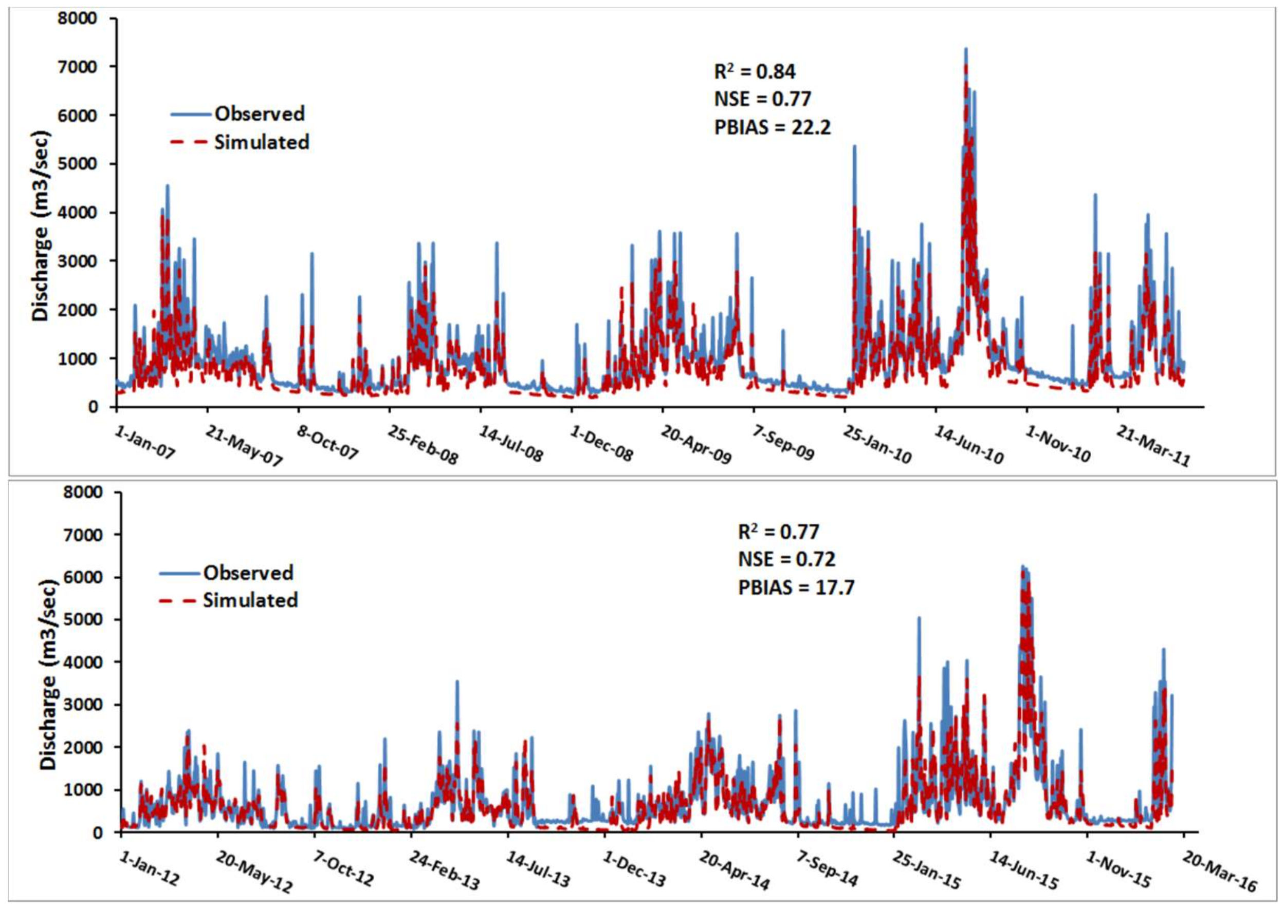
Figure 5.
Trends of flooding events in Kabul river. The blue dots are the observed flow recorded over the period of 1981–2015. The higher outlier during this analysis, which was actually the 2010 flood in this region. Y-axis represents the discharge of Kabul River in m3 s−1 while the primary X-axis shows the probability while the secondary X-axis shows the return period of the flooding in years. The red line shows the medium level flood (2800 m3 s−1) as described by the Federal Flood Commission of Pakistan.

Figure 6.
Variation in average monthly temperature (a–d), average monthly precipitation (e–h) and average monthly flow (i–l), all based on 20 years data for the Kabul river basin. When comparing observational data (1981–2000) and downscaled scenario data from four selected General Circulation Models (GCMs) under two Representative Concentration Pathways (RCPs) 4.5 and 8.5 in near (2031–2050, (a,b,e,f,i,j)) and far future (2081–2100, (c,d,g,h,k,l)).
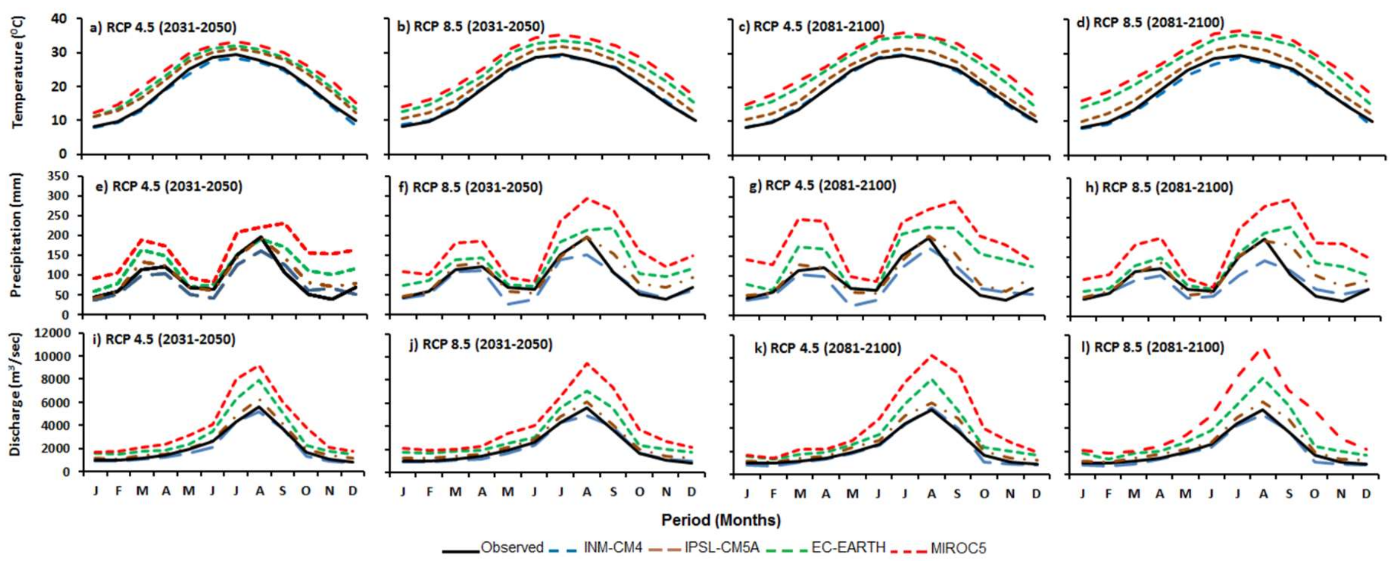
Figure 7.
Return periods of peak flow in Kabul river (years). Results for four different GCMs for the RCPs 4.5 and 8.5 for the near future (2031–2050, (a,c)) and far future (2081–2100, (b,d)) are presented. The horizontal dark brown line shows the magnitude of the most devastating flood in 2010.
Figure 7.
Return periods of peak flow in Kabul river (years). Results for four different GCMs for the RCPs 4.5 and 8.5 for the near future (2031–2050, (a,c)) and far future (2081–2100, (b,d)) are presented. The horizontal dark brown line shows the magnitude of the most devastating flood in 2010.

© 2018 by the authors. Licensee MDPI, Basel, Switzerland. This article is an open access article distributed under the terms and conditions of the Creative Commons Attribution (CC BY) license (http://creativecommons.org/licenses/by/4.0/).
Share and Cite
MDPI and ACS Style
Iqbal, M.S.; Dahri, Z.H.; Querner, E.P.; Khan, A.; Hofstra, N. Impact of Climate Change on Flood Frequency and Intensity in the Kabul River Basin. Geosciences 2018, 8, 114. https://doi.org/10.3390/geosciences8040114
AMA Style
Iqbal MS, Dahri ZH, Querner EP, Khan A, Hofstra N. Impact of Climate Change on Flood Frequency and Intensity in the Kabul River Basin. Geosciences. 2018; 8(4):114. https://doi.org/10.3390/geosciences8040114
Chicago/Turabian StyleIqbal, Muhammad Shahid, Zakir Hussain Dahri, Erik P Querner, Asif Khan, and Nynke Hofstra. 2018. "Impact of Climate Change on Flood Frequency and Intensity in the Kabul River Basin" Geosciences 8, no. 4: 114. https://doi.org/10.3390/geosciences8040114
Note that from the first issue of 2016, this journal uses article numbers instead of page numbers. See further details here.