A Database for Climatic Conditions around Europe for Promoting GSHP Solutions

Abstract

Weather plays an important role for energy uses in buildings. For this reason, it is required to define the proper boundary conditions in terms of the different parameters affecting energy and comfort in buildings. They are also the basis for determining the ground temperature in different locations, as well as for determining the potential for using geothermal energy. This paper presents a database for climates in Europe that has been used in a freeware tool developed as part of the H2020 research project named “Cheap-GSHPs”. The standard Köppen-Geiger climate classification has been matched with the weather data provided by the ENERGYPLUS and METEONORM software database. The Test Reference Years of more than 300 locations have been considered. These locations have been labelled according to the degree-days for heating and cooling, as well as by the Köppen-Geiger scale. A comprehensive data set of weather conditions in Europe has been created and used as input for a GSHP sizing software, helping the user in selecting the weather conditions closest to the location of interest. The proposed method is based on lapse rates and has been tested at two locations in Switzerland and Ireland. It has been demonstrated as quite valid for the project purposes, considering the spatial distribution and density of available data and the lower computing load, in particular for locations where altitude is the main factor controlling on the temperature variations.

1. Introduction

Ground Source Heat Pumps (GSHP) is a technology that promotes for the overall reduction of final and primary energy in buildings as well as diminishing the generated CO₂ emissions. Despite the potential of this technology, there are several problems that need to be resolved to promote a more extensive uptake and use of low temperature geothermal energy and increase the market share of GSHPs for heating/cooling buildings and communities. On the one hand, there is the need to reduce the installation costs of the Ground Heat Exchangers and increase public awareness of this technology. The work presented in this paper is part of a wider project (named Cheap-GSHPs) which aims to increase the use of GSHP systems, by decreasing installation costs, helping designers with proper design tools, provide information to stakeholders and end users interested in low temperature geothermal energy. Many tools for sizing ground source heat pump systems are available today, but they are usually aimed at expert users/designers. Moreover, the most accurate calculation methods are not freeware and cannot reach a wider audience and inhibiting the penetration of GSHPs to the heating and cooling market. To overcome this, three main tools are developed in the Cheap-GSHPs project:

• a design tool for expert users where the analytic method [1] and a numerical method [2] can be chosen;
• a Decision Support System (DSS) to help expert and non-expert users in assessing a first feasibility study on GSHP systems;
• an LCA tool to calculate the overall impact of a GSHP system and comparing it with standard HVAC solutions.

For all these tools a common platform is developed. This platform allows climatic conditions, energy demands of buildings, ground properties, a heat pump solutions repository as well as a renewable energy database to use in synergy with the GSHPs to be considered. Different approaches [3,4] are adopted in the development of these tools in order to address the different aims of the various tools. The DSS will generates different possible solutions based on a defined general problem and identifies the optimal solution. This means that the user defines few and simple inputs to generate an initial cost-benefit analysis and to check the feasibility of the GSHP solution. The design tool helps practitioners in the sizing of the ground heat exchangers [5]. This may be done in two ways: with a simplified approach (with a rough estimation of the overall heating and cooling demand of the building), or with a detailed calculation (either monthly based or hourly based). In the first option the tool generates a standardized pattern of heating/cooling loads; in the second option the user has to upload the previously calculated values of heating/cooling demands.

The DSS calculation is also based on the analytical method, hence the monthly energy needs of the buildings including the peak loads for heating and cooling have to be estimated. A database of buildings has been developed and integrated in the DSS to determine the average monthly pattern (hour by hour) of the energy loads. This is used in the numerical calculation method when the energy loads are defined on monthly basis by the user. More details on the approach used for finding the energy profiles can be found in Bernardi et al., 2016 [6].

The climatic conditions across Europe have been analysed based on the most common methodologies for defining the climate at a given location. The detailed calculation method used in the DSS considers also the very shallow heat exchange (ambient air, solar radiation, infrared radiation heat exchange with the sky) and requires the common platform to consider inputs including more complex and detailed weather characterization data. For this purpose the TRY (Test Reference Year) has been considered as basis for the climatic conditions database set up based on existing well established available libraries of TRY, i.e., ENERGYPLUS weather and METEONORM files. The common platform library can be enriched by the user by uploading general data for an available TRY specific to a location.

This paper focuses on the common platform that has been set up for the weather conditions. This considers simpler and more detailed climatic data based on a specific location as well as very detailed information. The analysis of the climates considered in the database developed is described hereafter.

1.1. Köppen Scale

Wladimir Köppen, a Russian-German scientist founder of modern climatology and meteorology, presented a first quantitative classification of world climates in 1900; Rudolf Geiger improved this world map in 1954 and 1961; thus the name Köppen-Geiger classification [7,8].

Köppen was first trained as a plant physiologist; as a consequence, he then realized that climate is responsible for plants distribution and diffusion. His effective classification was constructed based on the global vegetation map of Grisebach published in 1866 [7]. Sanderson and Thornthwaite claimed that Köppen’s use of the first five letters of the alphabet to label his climate zones comes from the five vegetation groups delineated by the late 19th century French/Swiss botanist De Candolle [9,10]. De Candolle in turn based these on the climate zones of the ancient Greeks. The five vegetation groups of Köppen distinguish between plants of the equatorial zone (A), the arid zone (B), the warm temperate zone (C), the snow zone (D) and the polar zone (E). A second letter in the classification considers the precipitation, a third letter the air temperature.

Essenwanger has provided a comprehensive review of the classification of climate from prior to Köppen through to the present [11]. Although various authors published enhanced Köppen classifications or developed new ones, the Köppen-Geiger classification is still the most frequently used [12,13,14].

Recently, four Köppen world maps, based on gridded data, have been produced for various resolutions, periods and levels of complexity. Kalvovà et al., using Climate Research Unit (CRU, the University of East Anglia) gridded data for the period 1961–1990, presented a map of the five major Köppen climate types at a resolution of 2.5° × 2.5° [15]. Gnanadesikan and Stouffer presented a Köppen map of 14 climate types based on the same CRU data and period, but at a resolution of 0.5° × 0.5° [16]. Fraedrich et al. 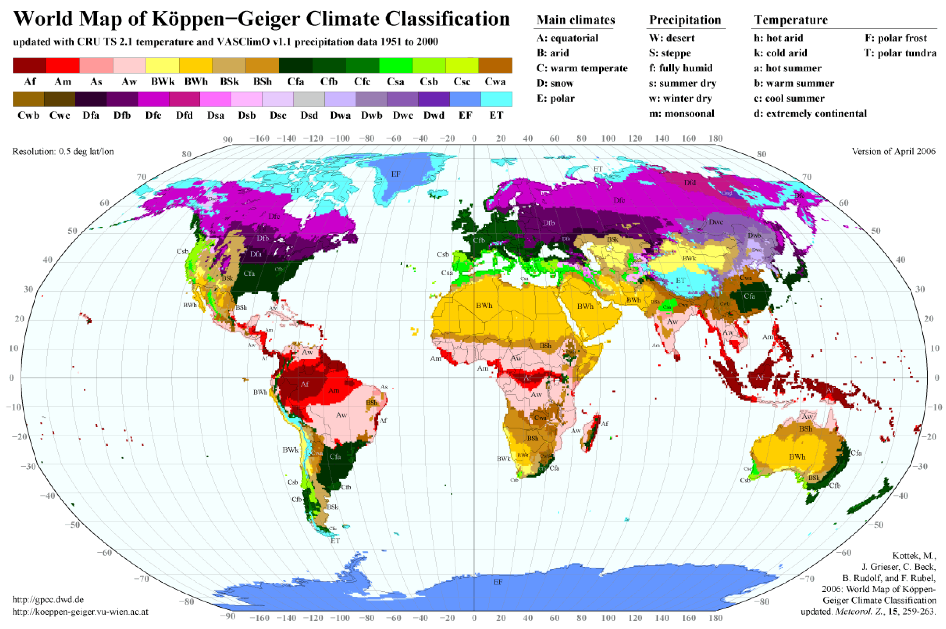[7] using CRU data for the period 1901–1995 presented a Köppen map of 16 climate types at a resolution of 0.5° × 0.5° and investigated the change in climate types over the period 1981–1995 relative to the complete period of record [17]. The most comprehensive Köppen world map drawn from gridded data to date is that of Kottek et al., who presented a map with 31 climate types at a resolution of 0.5° × 0.5° based on both the CRU and Global Precipitation Climatology Centre (GPCC) data sets of temperature and precipitation monthly record for the period 1951–2000 [18]; both data sets are freely available for scientific purposes (www.cru.uea.ac.uk; http://gpcc.dwd.de). The resulting world map depicted in Figure 1 corresponds quite well with the historical hand-drawn maps of the Köppen-Geiger climates, but shows more regional details due to the high spatial resolution and provides the opportunity for further investigations by applying the digital data.

The updated climate classification world map by Kottek et al. as well as the digital data are publicly available and distributed by the Global Precipitation Climatology Centre (GPCC) at the German Weather Service and the University of Veterinary Medicine Vienna [19,20].

All four maps based on gridded data cover restricted periods (1901–1995, 1961–1990 or 1951–2000) and any subgrid resolution climate type variability has been obscured. Peel et al. presented an updated world map of the Köppen-Geiger climate classification based on station data for the whole period of record based on a large global data set of long-term monthly precipitation and temperature station time series obtained from the Global Historical Climatology Network (GHCN) dataset [21]. In this work, climatic variables used in the Köppen-Geiger system were calculated at each station and interpolated between stations using a two dimensional (latitude and longitude) thin-plate spline with tension onto a 0.1° × 0.1° grid for each continent. Although broadly similar to the map by Kottek et al., the map by Peel et al. has a finer resolution and also deals with locations that satisfy two classification criteria simultaneously.

1.2. Degree Day for Heating and Cooling

Although the current standardized methods for determining the heating/cooling energy demand of the buildings can be based on quasi-steady state models (i.e., monthly based calculation method) or on dynamic models (based on hourly calculations), a simplified method for correlating standardized energy profiles of buildings may consider a simpler approach that has been widely used in the past, i.e., the so-called “Degree-days”. Degree-days provide a mean to compare energy performance in buildings under different conditions. Analysis techniques also use degree-days to produce empirical models of energy consumption [22]. The original Degree days concepts originated mainly within agricultural research to define the variation in outdoor air temperature [23].

Heating degree-day (HDD) is a type of measurement used in order to represent building energy loads devoted to ambient heating. HDD represent how much in terms of amount of °C and in terms of days, the air temperature is below a certain threshold value. This technique is also useful because the heating needs for a predefined building at a specific location can be evaluated as being directly proportional to the HDD values at that location. In the same way, the value of cooling degree-day (CDD), reflects the amount of energy used for building cooling, by considering information regarding how much in terms of °C and in terms of days the air temperature is above a certain threshold [24,25]. Weekly or monthly degree-day figures may be used in energy monitoring to determine the heating and cooling costs of climate controlled buildings, whilst annual figures can be used for estimating projected costs [26].

A degree-day must be calculated as the integral of a function of time f(t) that changes with temperature. The function f(t) is truncated to upper and lower limits that are appropriate for climate control. The f(t) function can be projected or measured according to one of the available methods in literature [26]. A key issue in the application of degree-days, is the definition of the base temperature in buildings that relates to the energy balance of the building and system.

HDDs are defined by taking into account a certain base temperature, i.e., the outside temperature above which a building needs no heating. The most appropriate base temperature for any particular building depends on the temperature that the building is heated to. This is dependent on the type of the building and needs to consider the heat-generated by occupants and equipment within it (internal gain). The base temperature is usually an indoor temperature of 18–19 °C, which is adequate for human comfort (internal gains increase this temperature by about 1–2 °C).

Recent publications by the CIBSE and The Carbon Trust provide a current view of the theory and application of heating degree-days [26,27,28]. The CIBSE publication replaces previous guidance [26] and provides a detailed explanation of the concepts described above setting out the fundamental theory upon which building related degree-days are based. It demonstrates the ways in which degree-days can be applied and provides some of the historical backdrop to these uses.

Calculations using HDD present some warnings and have to be used taking into account some specific cautions. Heat requirements are not always linear with temperature and heavily insulated buildings having a lower “balance point” [29,30]. The amount of heating and cooling needs depend on several factors besides outdoor temperature. These include: building insulation, amount of solar radiation, number of electrical appliances running, wind speed outside the building and comfort temperature of the occupants. Another important factor in determining human comfort is the amount of relative indoor humidity. Other variables such as precipitation, cloud cover, heat index, building albedo and snow cover can also alter a building’s thermal response. Another issue with HDD is that care needs to be taken if these are to be used to compare climates internationally, because of the difference in standard baseline temperatures used in different countries.

With regard to CDD, the methodology has not been so far well developed despite having been published and cited in many papers and works. : For this reason, their use in connection with cooling or air-conditioning of buildings should be carefully weighted [28,31]. Latent load is an important factor in determining the overall cooling energy demand of the building, but is difficult to estimate based on CDD e. This is particularly true when dealing with a building which is not known or if calculations have to be based on CDD only. In this paper HDD and CDD have been used as a base to create correlations for providing information on a set of buildings with energy needs for heating and cooling that have been previously calculated by dynamic building simulations. The following paper presents the use of HDD and CDD to interpolate the sensible energy need of heating and cooling for a set of buildings located in different climates throughout Europe [32].

2. Material and Methods

2.1. Data Analysis

The weather definitions explained above are used to create a climate database for integration in the tool used for sizing the Ground Source Heat Pumps (GSHPs) as well as the Decision Support System (DSS) which are developed in the Cheap-GSHPs project [33,34,35].

Turban et al. (2005) broadly define a DSS as: “a computer-based information system that combines models and data in attempt to solve semi-structured and some unstructured problems with extensive user involvement” [36]. This information system requires hardware and software components plus a series of human elements such as designers and end-users to live. The system’s final aim is to support decision-making, by providing the stakeholders at all the level with a series of scenario. The Cheap-GSHPs project has developed a DSS tool aimed designers and building owners to accelerate the decision making process as well as increasing market share of the Cheap-GSHPs technologies.

The database is built up in terms of synthetic values that can be easily understood by expert and non-expert users. For this reason, two main parameters have been chosen:

• The Köppen-Geiger scale helps to select the climate similar to the location being investigated.
• The degree-day (DD) for heating (HDD) and cooling (CDD) shows an expert user if the location requires mostly heating or cooling or both.

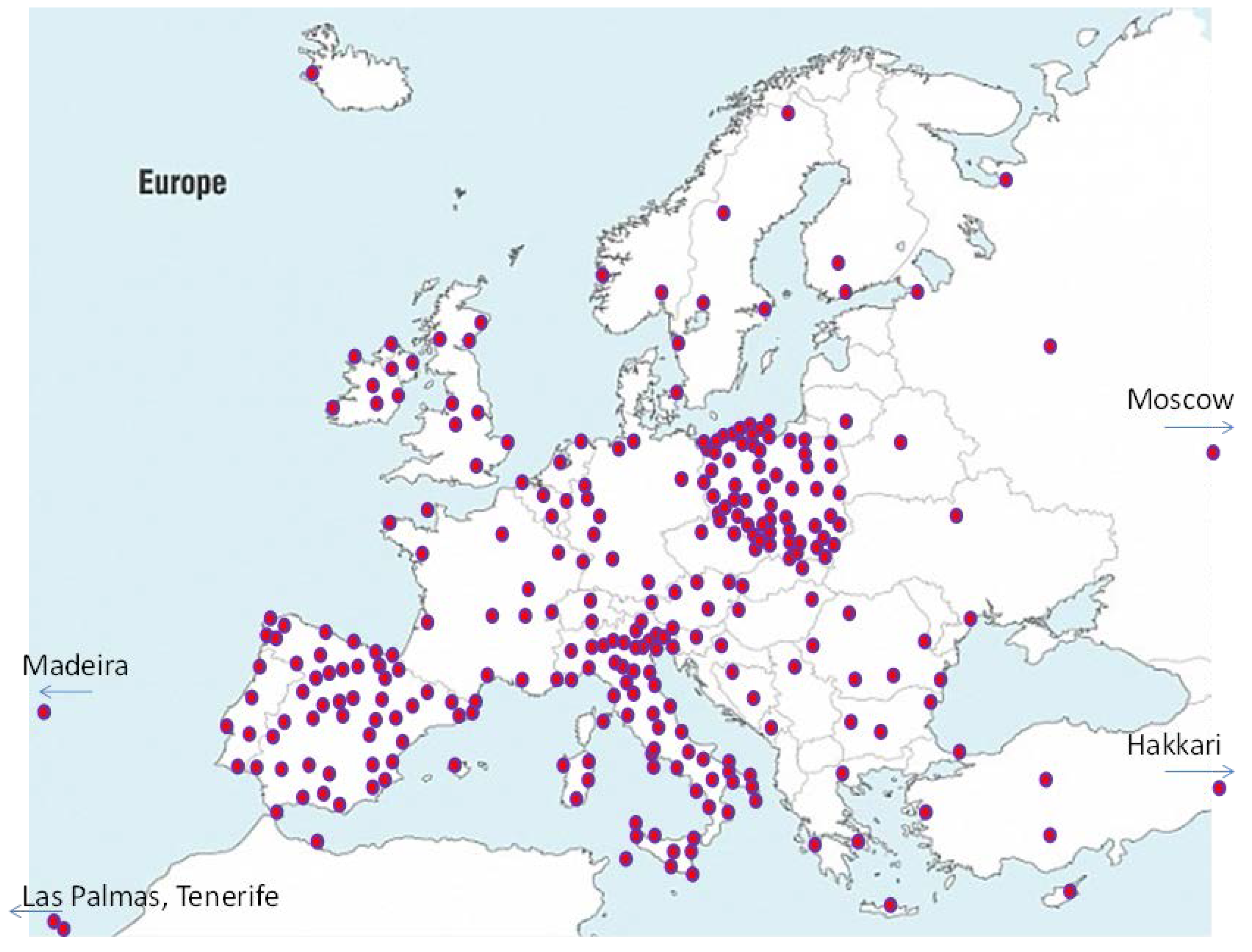
Firstly, a suitable set of data has been produced by using the Test Reference Year (TRY) included in the database of METEONORM and ENERGYPLUS software. Figure 2 shows the locations selected from both databases to create a European wide database.

By comparing the locations and the Köppen-Geiger map of Europe (Figure 3), a good definition of most of the climate classes is achieved (

Table 1. Number of locations included in the database in relation to the Köppen-Geiger climate classification.

Type of Climate	Description	Amount of Locations
BSk	Arid, summer dry, cold air	6
BWh	Arid, desert, cold air	2
Cfa	warm temperature, fully humid, hot summer	25
Cfb	warm temperature, fully humid, warm summer	133
Cfc	warm temperature, fully humid, cool summer	1
Csa	warm temperature, summer dry, hot summer	72
Csb	warm temperature, summer dry, warm summer	25
Dfa	Snow, fully humid, warm summer	37
Dfb	Snow, fully humid, cool summer	6

).

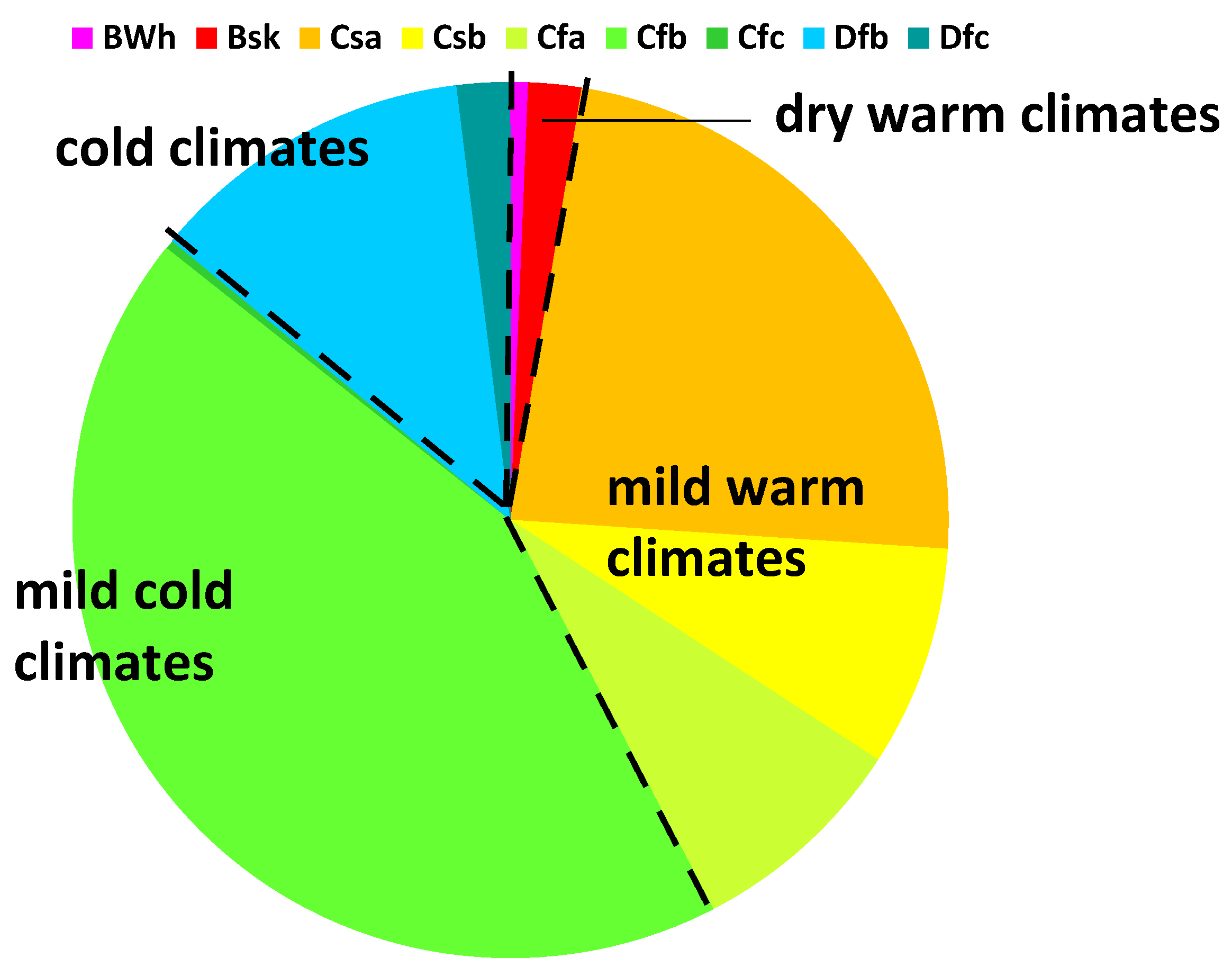
The cities grouped into these categories have been further analysed to assess how to define simpler information for non-expert users. For this purpose, based also on the values of the HDD and CDD, the following macro-groups have been defined (Figure 4):

• Dry warm climates, including BWh and BSk
• Mild warm climates, including Csa, Csb, Cfa
• Mild cold climates, including Cfb and Cfc
• Cold climates, including Dfb and Dfc

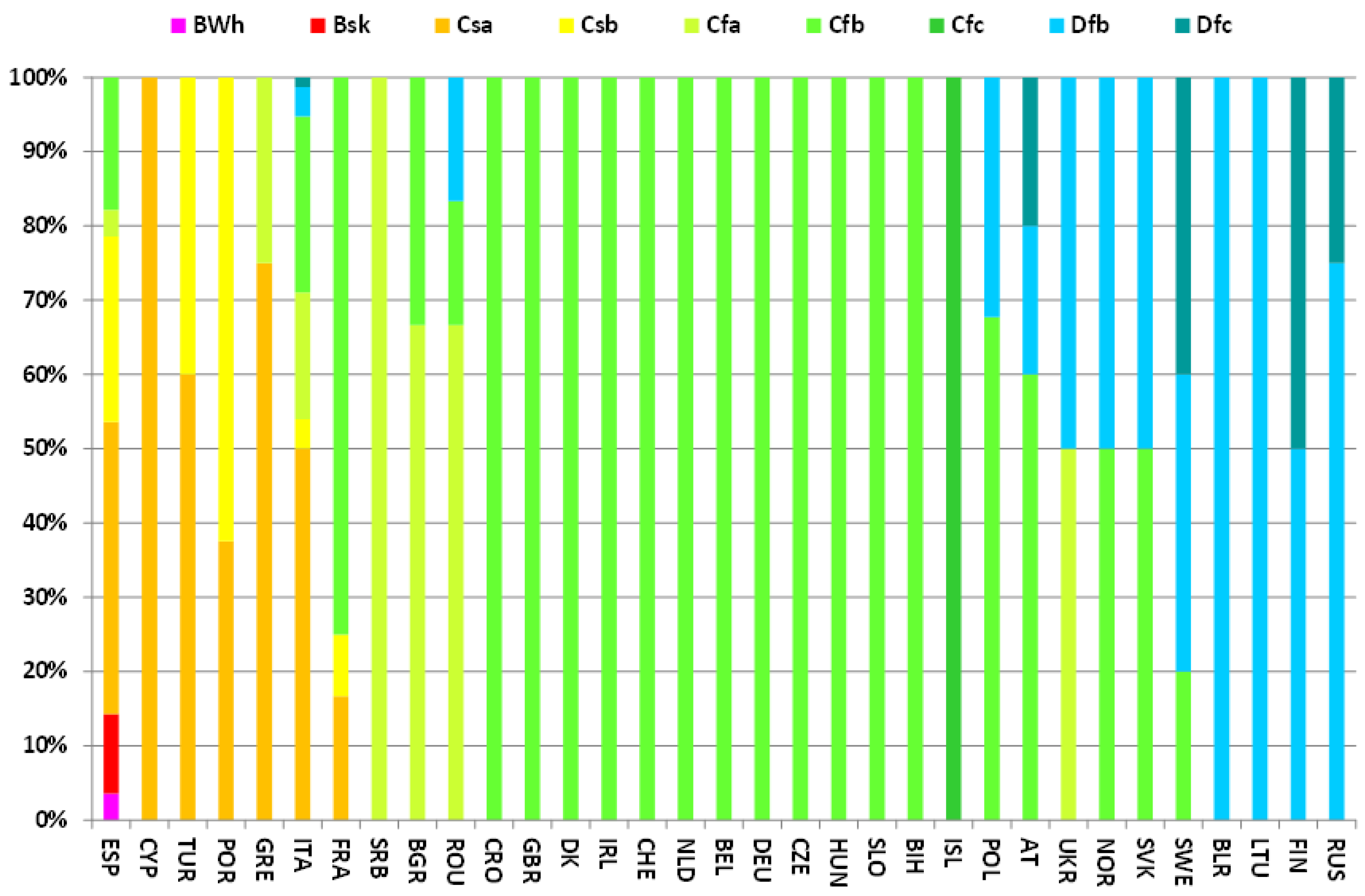
A further analysis has been carried out for each country in order to see whether there were differences in the climate depending on particular conditions. Figure 5 shows the overall results listing the climate conditions per country from the warmest climates to the coldest climates. This provides a quick overview on what can be expected in a certain country in terms of climate conditions and hence as potential for heating and/or cooling.

For the degree-day for heating and cooling, different definitions and set of conditions are proposed in literature. The following equations have been used for the calculations:

$$HDD= {\sum }_i\left(18-t_{ext, i}\right) \mathrm{if} t_{ext, i}<14,$$

(1)

$$CDD= {\sum }_i\left(18-t_{ext, i}\right) \mathrm{if} t_{ext, i}>20,$$

(2)

where $t_{ext, i}$ is the average external temperature for each day and the sum is extended all over the year.

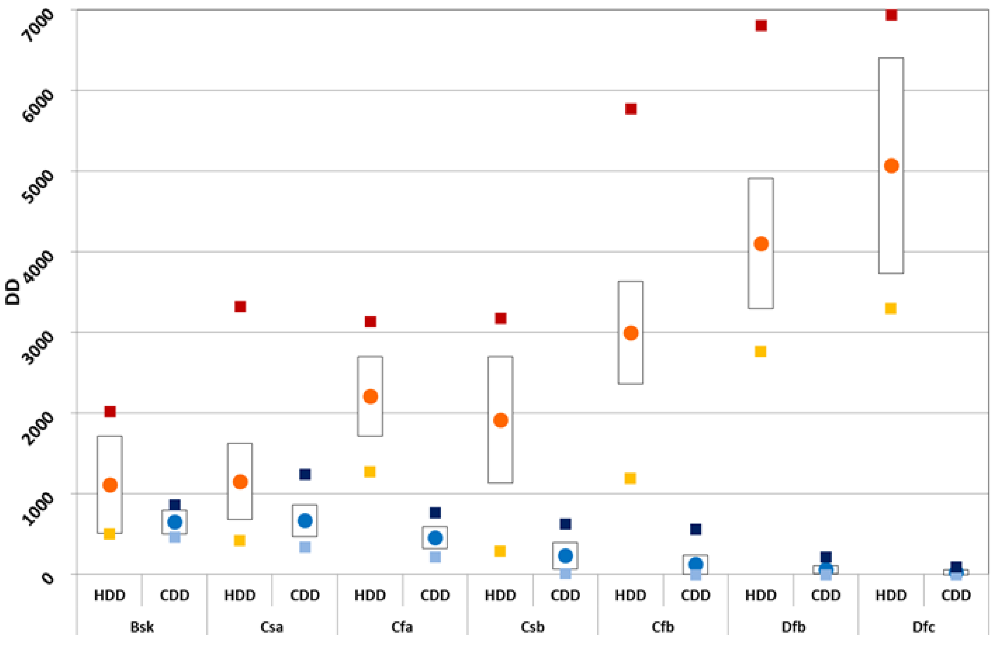
Based on the calculated DD for heating and cooling for each location included in the combined ENERGYPLUS and METEONORM database, a statistical analysis has been carried out. Due to the limited values for BWh (only two locations in Canary Islands) and Cfc (only Reykjavik), the analysis has been carried out only for the Bsk, Cfa, Cfb, Csa, Csb, Dfb, Dfc climates. Figure 6 shows, the average values of the HDD (orange circles) and CDD (blue circles) for each climate class, as well as the standard deviation (bars around the mean values). In the same figure, the minimum (yellow squares) and maximum (red squares) HDD values, as well as the minimum (light blue squares) and maximum (dark blue squares) CDD values, are also reported for each climate class.

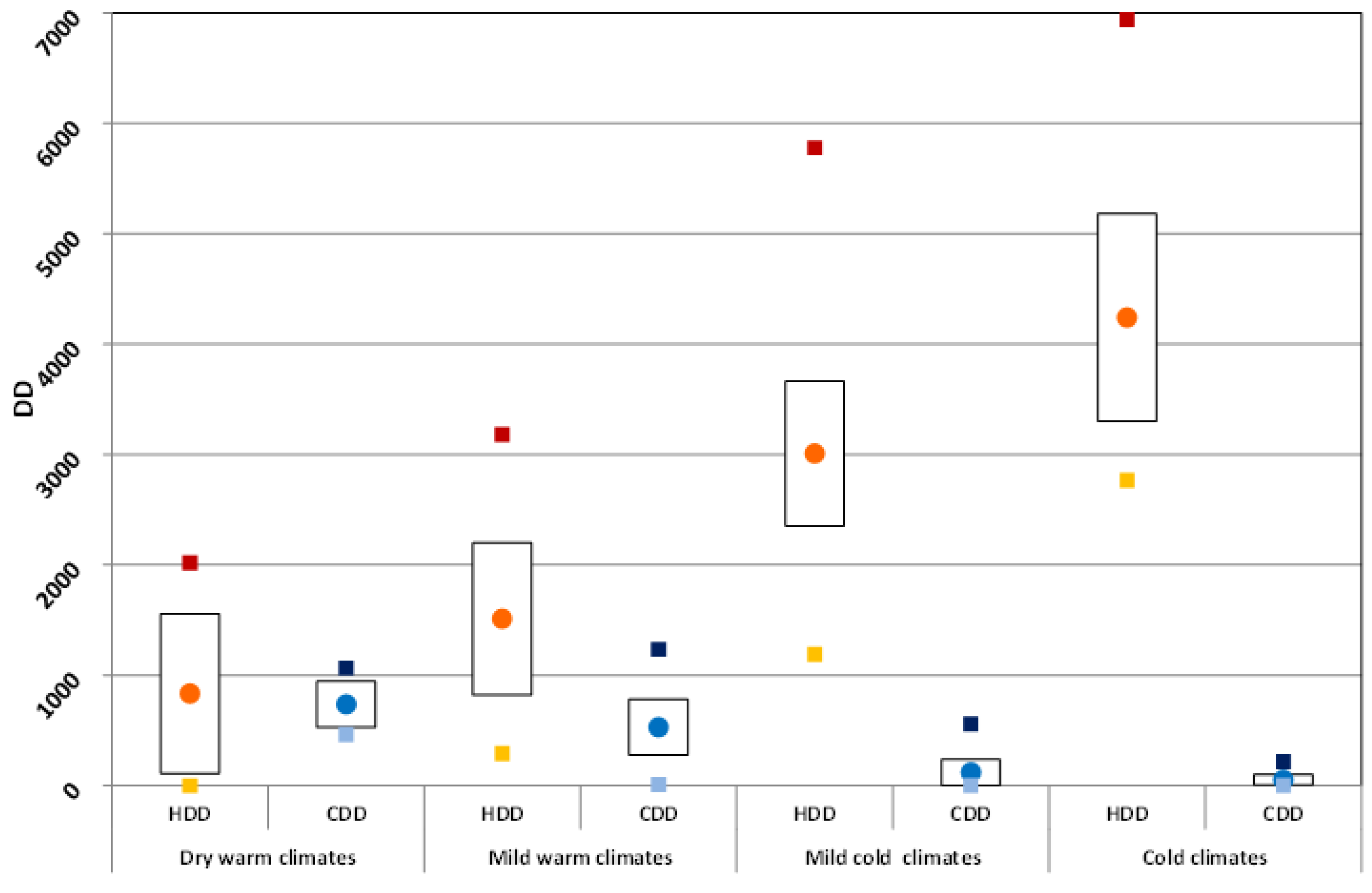
The statistical analysis for HDD and CDD has been also applied to the macro-groups as defined above (dry warm climates, mild warm climates, mild cold climates, and cold climates). The results are shown in Figure 7 for the average values of the HDD (red circles) and CDD (blue circles); the standard deviation (bars around the mean values) is also reported. In the same figure the minimum (yellow squares) and maximum (red squares) HDD values, as well as the minimum (light blue squares) and maximum (dark blue squares) CDD values, are also reported for each main climate class.

This simplified classification is easier and shows a more evident trend in the increase of HDD and decrease in CDD when passing from dry warm climates to cold climates.

2.2. Altitude Correlation

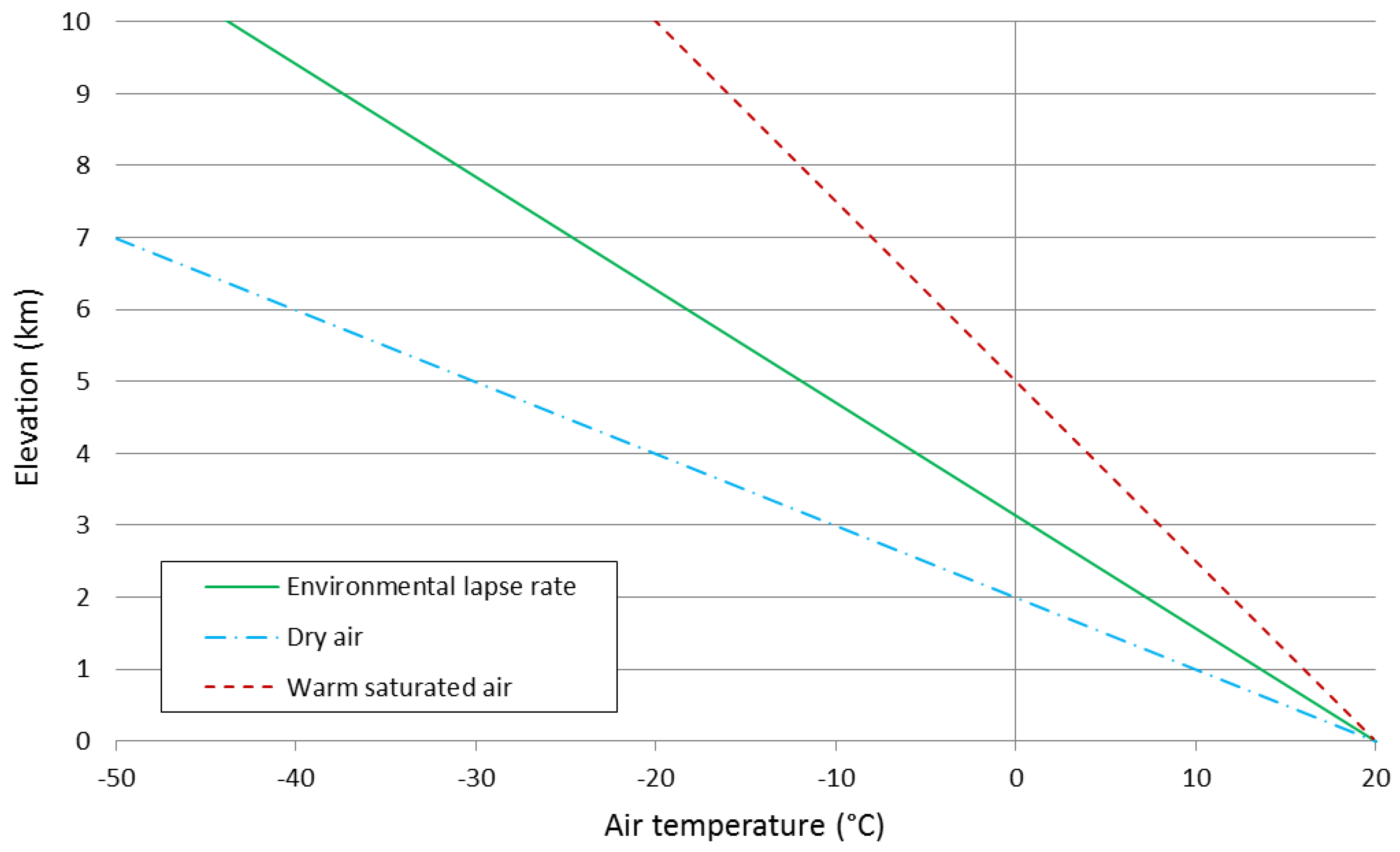
The surface air temperature measured by meteorological stations is a function of several factors among which latitude (which in turns determines solar incident radiation), cloud cover, continental/maritime effects, ocean currents and altitude [37,38]. Altitude, in particular, plays an important role in affecting air temperature. As air masses are forced to ascend in the atmosphere, they expand and cool as result of pressure decrease. The rate at which the air cools is known as lapse rate. If no heat is exchanged with the outside system during the process, cooling is adiabatic. Lapse rate is not constant and several factors affect it. The lapse rate varies from −9.8 °C/km for dry air (adiabatic lapse rate) to −4.0 °C/km for very saturated and warm air (saturated adiabatic lapse rate). However, the process is rarely adiabatic and some heat exchange occurs. The actual lapse rate at a given place is called environmental lapse rate and a typical value used for its global mean is −6.5 °C/km (Figure 8). However, lapse rates fluctuate at many scales: seasonally, diurnally and regionally and in the case of temperature inversions may even change sign [39,40].

Aside from the above-described height effect, in mountain regions a phenomenon known as orographic uplift occurs. The overall effect of altitude on air temperature is manifested by cooling with increasing elevation of the location, as air masses have to rise because of the topographic obstacles represented for instance by hills and mountains.

Air temperature measured in specific meteorological stations may be also affected by local factors and processes operating at different temporal and spatial scales, i.e., topographic barriers, presence of lakes and other water bodies, wind, orientation of topographic surface and cool air ponding (among others).

Temperature is measured in stations built and operated according with standards issued by the World Meteorological Organization [41]. However, as often occurs with environmental variables, continuous spatial prediction of “spot” measured values is necessary for modelling biological, environmental and physical processes. This is particularly true for air temperature, a key parameter to assess the heating and cooling needs of buildings.

Since buildings may be located in areas distant from meteorological stations, spatial interpolation is necessary to acquire temperature values by using data from nearby or known meteorological stations. According with Burrough and McDonnell, spatial interpolation is defined as predicting the values of a primary variable at points within the same region of sampled locations, while predicting the values at points outside the region covered by existing observations is called extrapolation [42].

A comprehensive review of available spatial interpolation methods used in environmental sciences is provided by Li and Heap [43]. They analysed 25 spatial interpolation methods providing a decision tree to support the selection of the most suitable, taking account data availability, data nature, expected estimations and features of the method.

2.3. Air Temperature Modeling

According to the same authors, almost all methods analysed in their work, rely on some form of equation:

$$\widehat{z}\left(x_0\right)= {\sum }_i^n{\lambda }_{i}z\left(x_i\right),$$

(3)

where $\widehat{z}$ is the estimated value of the primary variable at the point of interest $x_0$; $z$ is the observed value at the sampled point $x_i$; ${\lambda }_i$ is the weight assigned to the sampling point; n represents the number of sampled points used for the estimation.

The methods in turn can be classified in:

• Non geostatistical;
• Geostatistical (Univariate and Multivariate);
• Combined methods;

Numerous authors worked on temperature interpolation applying several tools to acquire distributed temperature models with different spatial and temporal resolution. Holdaway used Kriging to model and interpolate monthly average temperature [44,45]. Dodson et al. and many other authors, by using a Neutral Stability Model and Linear Lapse Rate [37,46,47,48] Adjustment algorithms, were able to obtain a high resolution model for daily air temperature over a large mountain region. Recently, Andrade-Berjano used linear mixed models for monthly average temperature interpolation in an intertropical region that allowed to parameterize and model temperatures in presence of ENSO (El Niño Southern Oscillation) and La Niña phenomena [49]. Frei proposed a method for the interpolation of mean annual and mean monthly air temperatures using non-linear profiles and non-euclidean distances in mountainous regions [50]. This kind of interpolation can deal with cool ponds and temperature inversion, a phenomenon known to occur in those areas.

In all cases, the topography of the analysed areas results to be an important factor affecting the performance of some interpolation methods: Kriging, IDW, two dimensional splines and trend-surface regressions, for example, work well in relatively flat homogeneous terrain. The strong relation between temperature and elevation precludes a simple interpolation with geostatistical methods in mountainous terrain unless the effect of elevation on temperature is explicitly taken into account [46,48]. Furthermore, in some cases, it has been suggested that regression models work better in mountainous regions than more complex approaches [51,52].

When modelling temperature/altitude relation from point-based data, an important factor that must be considered is that the locations of meteorological stations tend to be biased towards lower elevations [46,47].

Li and Heap compared some non-geostatistical and geostatistical methods in temperature estimation for three temporal scales: 10 years average, seasonal and daily in two regions [43]. Stronger correlations between elevation and temperature favoured Linear regression Model (LM) and Lapse Rate (LR). However, LM, LR and Co-Kriging (CK) were inappropriate when correlation between temperature and elevation was below 0.72. Inverse Distance Squared (IDS), Optimal Inverse Distance (OID), and Kriging showed similar robustness to a priori data range, correlation (between elevation and temperature) and variance. Splines seemed to be most sensitive to a priori data characteristics, among all the assessed methods. Kriging was favoured over OID when data was anisotropic. When data was isotropic, Optimal Inverse Distance Weighting (OIDW) was favoured. When data variance was high, or correlation between temperature and elevation was low, CK produced specking or “bird’s eye” effects around station locations. While the LR performed poorly in terms of mean absolute error, its results were more plausible than methods that did not use elevation as ancillary information. This was especially true where station elevations were not representative of regional elevations. LR was preferable over CK based on visual plausibility and adherence to the original data range. While preferable over CK, the LR method showed some banding effects and island-like isothermal tessellations around certain influential stations. Outlier stations were less noticeable with polynomial regression than with the LR [53].

2.4. Proposed Algorithm to Obtain Temperature Data in Unknown Locations from Nearby Weather Stations at Different Altitude

As discussed in the previous section, temperature values prediction is a complex issue that can be analysed by using different approaches and instruments. We propose to use lapse rate (also named smart interpolation) as the method to estimate air temperature in relation to elevation [43,53,54,55,56,57,58].

The lapse rate method uses the relationship between temperature and elevation for a region to estimate temperatures at unsampled sites. Typically, temperatures decrease as elevation increases, as previously described. The lapse rate method uses the temperature values of the nearest weather station and the difference in elevation to estimate the temperature at the unsampled site. To estimate temperature at an unsampled site, the difference in elevation is multiplied by the lapse rate and the subsequent number is added to or subtracted from the weather station temperature to yield the site temperature [53], according with the following equation proposed by Stahl et al. [47,59]:

$$T_p=T_0+\lambda \left(h_p-h_0\right),$$

(4)

where $T_0$ is the nearest known temperature; $T_p$ is the temperature at the prediction point; $\lambda$ is a specified temperature gradient expressed in °C/m; $h_p$ is the elevation in meters of the prediction point; $h_0$ is the elevation in meter of the predictor station.

Specified lapse rates are calculated monthly by identifying pairs of low-elevation, high-elevation stations close to the interested point and computing vertical temperature gradients.

The basic assumption of this method is that lapse rate is constant across the study region [43]. When elevation and temperature are not correlated, then the lapse rate method degrades into a Nearest Neighbour (NN) method, where interpolated values simply take on the value of the nearest station point [43,60].

By using this approach Stahl et al. were able to model daily maximum and minimum air temperature in a region with complex topography, highly variable station density and altitude distribution [59]. However, none of the 12 models tested by the authors in their work was able to predict the full range of daily maximum and minimum temperature, underestimating and overestimating high and low temperatures respectively.

2.5. Testing of the Proposed Method and Results

To assess the soundness of the approach, we tested the LR method against four different datasets from different climates and countries: in particular, we analysed locations placed within Cfb and Csa climates, which represent the most frequent climates in the database (see Table 1). These countries have been also selected because they represent distinct climatic and topographic conditions. The Swiss territory is characterised by strong altitudinal gradient, while in Ireland the altitude gradient is not as relevant as in Switzerland and a strong influence from the Atlantic Ocean is observed. The same phenomenon is also observed in Greece with the Mediterranean Sea, while central Spain can be described as an average continental background, without the extremely high elevations of Switzerland. Test for Switzerland has been performed using monthly data temperatures from MeteoSwiss pertaining to 1981–2010 climatic normal (www.meteosvizzera.ch). The method was developed and tested for DSS implementation: this means that the results provided by the proposed method take into account only yearly values or monthly profiles of average air temperature. A more detailed reconstruction of daily or hourly data using this method is not recommended, as air temperature data is affected by many other variables along with elevation [39]. The results of the analysis are reported in the supplementary material as spread sheet.

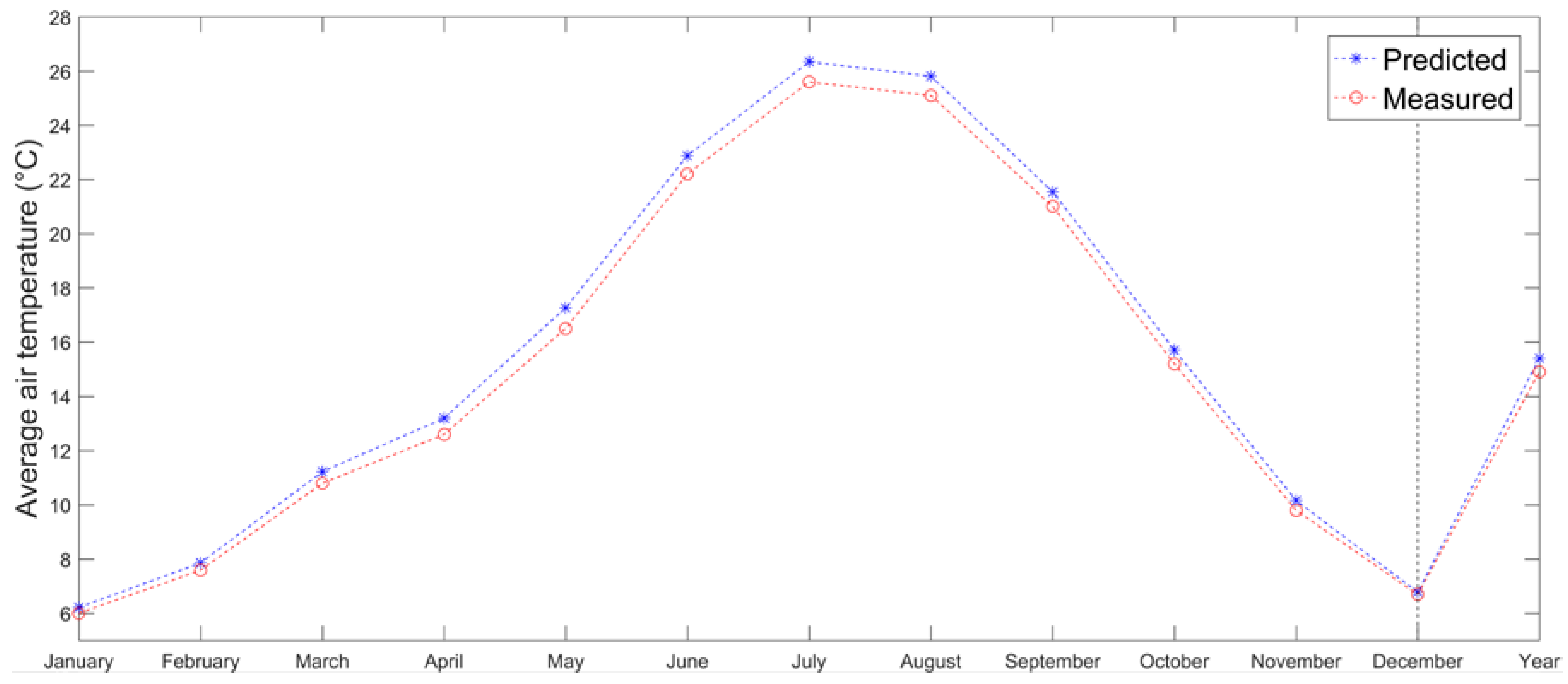
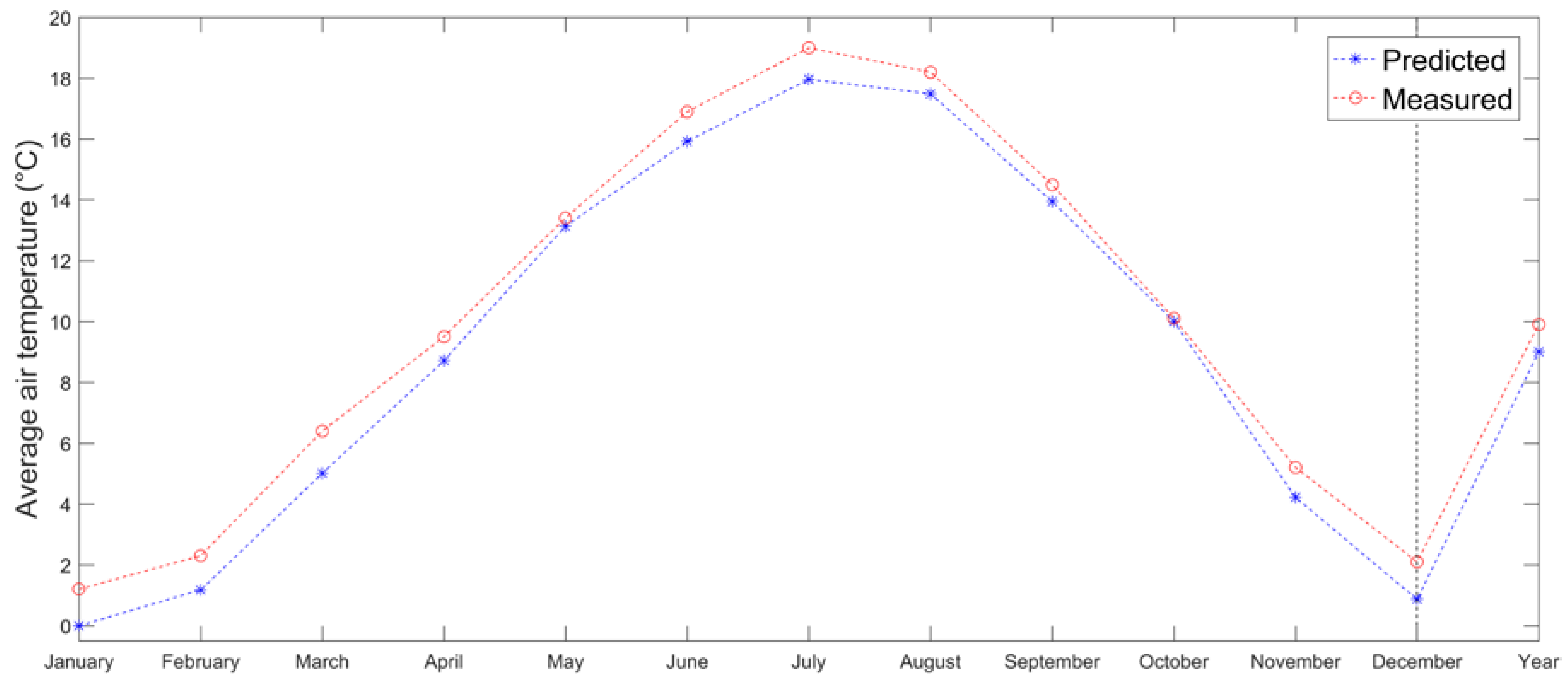
Estimation of monthly mean temperatures at Acquarossa meteorological station (575 m a.s.l.) in Switzerland has been performed using Engelberg as the predictor station (1036 m a.s.l.). Monthly lapse rates have been obtained by using 4 pairs of stations placed nearby (excluding the predictor) at higher and lower altitudes. All stations have been selected in the southern part of the Alps. The LR method seems to generally underestimate temperatures for Acquarossa (Figure 9). However, the differences between measured and estimated temperatures are less than 1 °C in all months, MAE is quantified in 0.87 °C and RMSE in 0.94 °C.

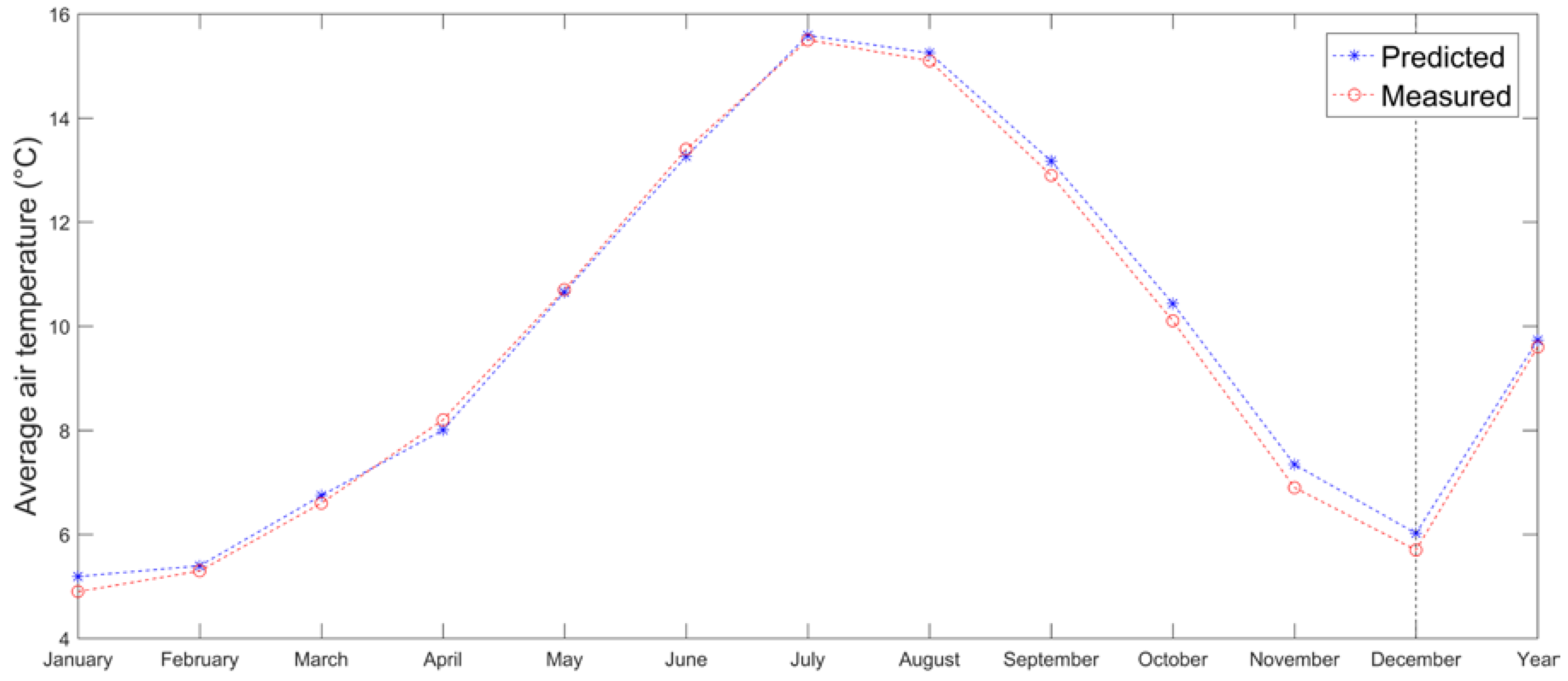
The same approach has been tested for Ireland to estimate monthly mean air temperatures at Birr meteorological station (73 m a.s.l.), by using values from Casement station (94 m a.s.l.). Irish data comes from the Irish Meteorological Service (www.met.ie) describing 1971–2000 climate normal. Monthly lapse rates have been calculated from four stations in the area excluding the predictor one. Although the results seem similar to those obtained for Acquarossa and globally better (MAE and RMSE are equal to 0.2 and 0.23 °C), there are remarkable differences (Figure 10). Monthly lapse rates present larger variations (supplementary material) with values above 14 °C/km. Hence, factors different from the altitude control temporal and spatial variation of air temperature in this area.

Two more locations and their respective climatic normal series were analyzed and tested against the LR method: Spain and Greece. The climatic normal 1981–2010 for Spain was retrieved from the Agencia Estatal de Meteorología (AEMET: http://www.aemet.es) website. Here the proposed approach was used to estimate the average air temperatures for Madrid Cuatro Vientos (690 m.a.s.l.) meteorological station, by computing the lapse rate for 4 pairs of stations, excluding the predictor one, which is represented by Getafe station (620 m.a.s.l.). The results are quite good also in this case, since the MAE and RMSE are quantified respectively in 0.49 and 0.53 °C. In this case the method tends to slightly overestimate values (Figure 11).

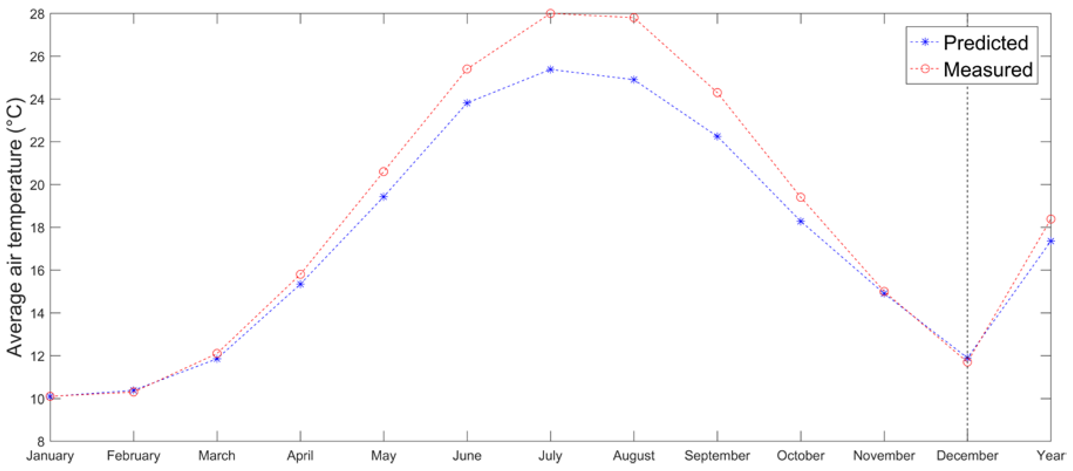
For Greece, a climate series collected from the Hellenic National Meteorological Service (www.hnms.gr/emy/en/index_html), describing 1971–2000 climate values was used. The average lapse rate have been calculated for 4 pairs of stations excluding the predictor one, which is represented by Skyros station (18 m.a.s.l.). The procedure was applied to estimate the average air temperature of Athens Elliniko (47 m.a.s.l.). Results are also in this case quite satisfying, since the MAE and RMSE between measured and calculated are respectively of 0.7 and 0.86 °C. Only July and August show a relevant error (approximately 1.6 and 1.7 °C), but the overall accuracy is good, even for the annual average. The applied method tends to underestimate values in this case (Figure 12).

The method proved to be reliable for the purposes of the work and of the Cheap-GSHPs project, given its replicability on a European-wide scale.

3. Discussion and Conclusions

The climate conditions of Europe have been analysed based on the database of ENERGYPLUS and METEONORM. For each location, the Köppen-Geiger scale, as well as the HDD and the CDD have been evaluated. The climate conditions have been further subdivided in four macro-groups: dry warm climates, mild warm climates, mild cold climates and cold climates. This subdivision may be easier to understand and helps non-expert users to check which climate can be considered similar to a location of interest. The HDD and CDD are necessary for designers in order to measure the heating and cooling potential of building. Based on HDD and CDD, the energy needs of buildings can be estimated, as shown in Badenes et al., according to standardized calculated heating/cooling profiles [32]. Moreover, the HDD and CDD, coupled with the described climate macro-groups, offer an efficient method of determining a more detailed climate outline for every location.

As result of this work, a comprehensive database of climate conditions for Europe is provided for the development of further analysis within the EU project Cheap-GHPs. The database is available as supplementary material. It is composed of

• TRY from ENERGYPLUS and METEONORM data sets;
• Data set of calculated degree-days for heating and cooling;
• Köppen-Geiger climate classification;
• Macro-climatic subdivision
• Data input from the user;
• Estimation of temperatures at unknown locations.

For the last task, the lapse rate (LR) method can be used to predict temperatures at unknown locations by using information of a nearby station and the altitude difference between the predictor station and prediction location, meaning that the temperature for unknown location can be estimated by interpolation of nearby stations, taking into account the relative differences in altitude. The error of LR method is in general greater if compared with other methods, but no sensible gain in precision is expected by using more complex methods due to the spatial distribution and density of available data. In addition, methods that are more complex may require more parameterization, thus introducing additional sources of error. Using LR requires less computing load if compared with other methods.

An advantage of using the nearest station to estimate the temperature is that the closer the stations are to the target location, the more likely similar climatic characteristics can be characterized. Then, the probability of having differences due to local effects (i.e., in presence of orographic barriers in between) is minimized, although not completely removed.

By using LR, it would be possible to estimate also daily maximum and minimum temperatures, but since daily temperatures tend to be much noisier and influenced by other factors (cold pools, inversions etc.), they are more difficult to estimate and interpolate than monthly or annually averaged air temperature data [46].

In places where other factors aside from altitude affect the variation of temperature, Nearest Neighbour or other geostatistical methods may be used for the estimation of local temperature. In areas characterized by few meteorological stations to compute monthly lapse rates and with strong altitudinal gradients, an environmental “fixed” lapse rate could be used for predictions.

Possible steps to be followed when applying LR method in this project are:

• The user provides the coordinates and altitude of the location of interest with unknown climatic information;
• The tool should search within increasing radius from the provided coordinates to get at least one pair of meteorological stations being one below and the other above the altitude provided by the user. The research for meteorological stations should be stopped at a fixed distance from the location proposed by the user (e.g., 300 km, a proposal to be tested during tool development), or when a fixed number of suitable pairs are reached (e.g., 10 pairs, proposed value);
• Pairs of stations being both at lower or both at higher altitudes than one of the user input should be discarded;
• The tool performs the calculation of the monthly lapse rates using only pairs of stations placed one at lower and one at higher altitude from the user input;
• If more than one pair of stations is available, the tool calculates the mean lapse rate for each month to obtain monthly mean temperature at the user location.

Wherever this approach is not applicable (i.e., locations below the lowest or above the highest available meteorological stations, places where the distance of the meteorological stations beyond the maximum value attributed to the search radius would not be representative; areas where other factors different than lapse rate control temperature variations), the tool may allow using a fixed “environmental” lapse rate of −6.5 °C/km or eventually a user defined value.

Further data and information are available at the Cheap-GSHPs project website (http://cheap-gshp.eu/).