Flood Hazard Management in Public Mountain Recreation Areas vs. Ungauged Fluvial Basins. Case Study of the Caldera de Taburiente National Park, Canary Islands (Spain)

 ,
,  ,
,  ,
,
Abstract
:1. Introduction
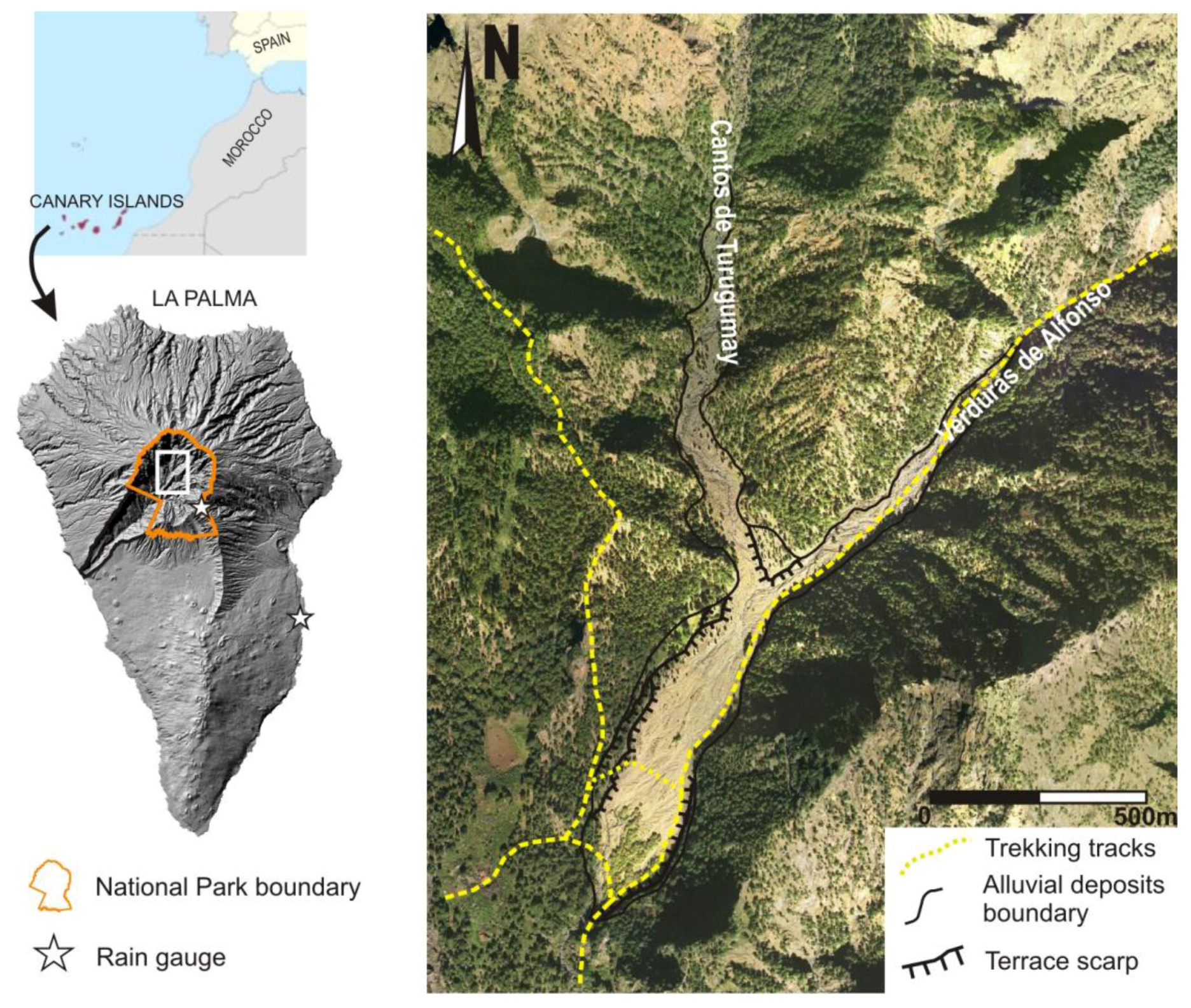
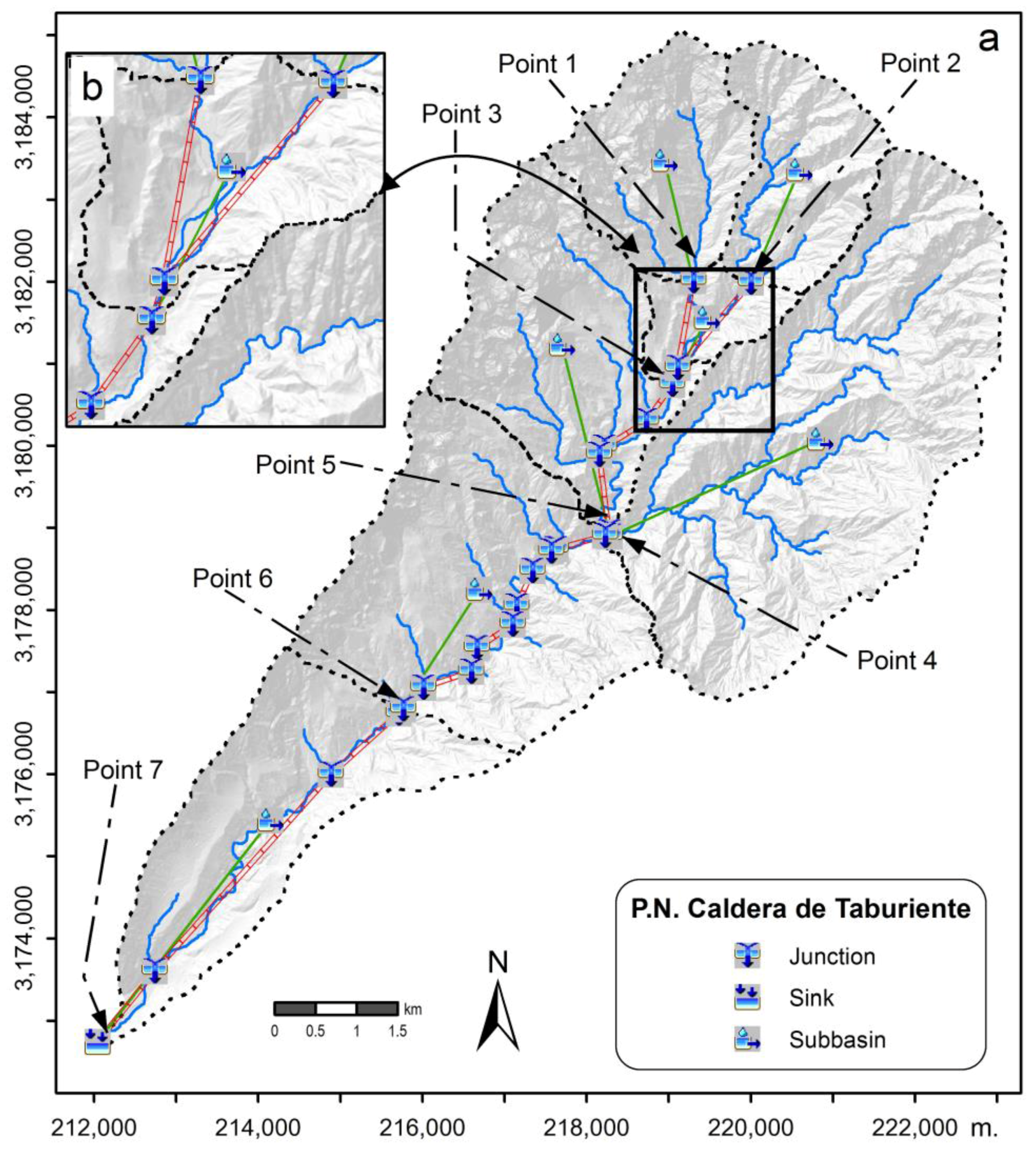
2. Case Study Area
2.1. Geology
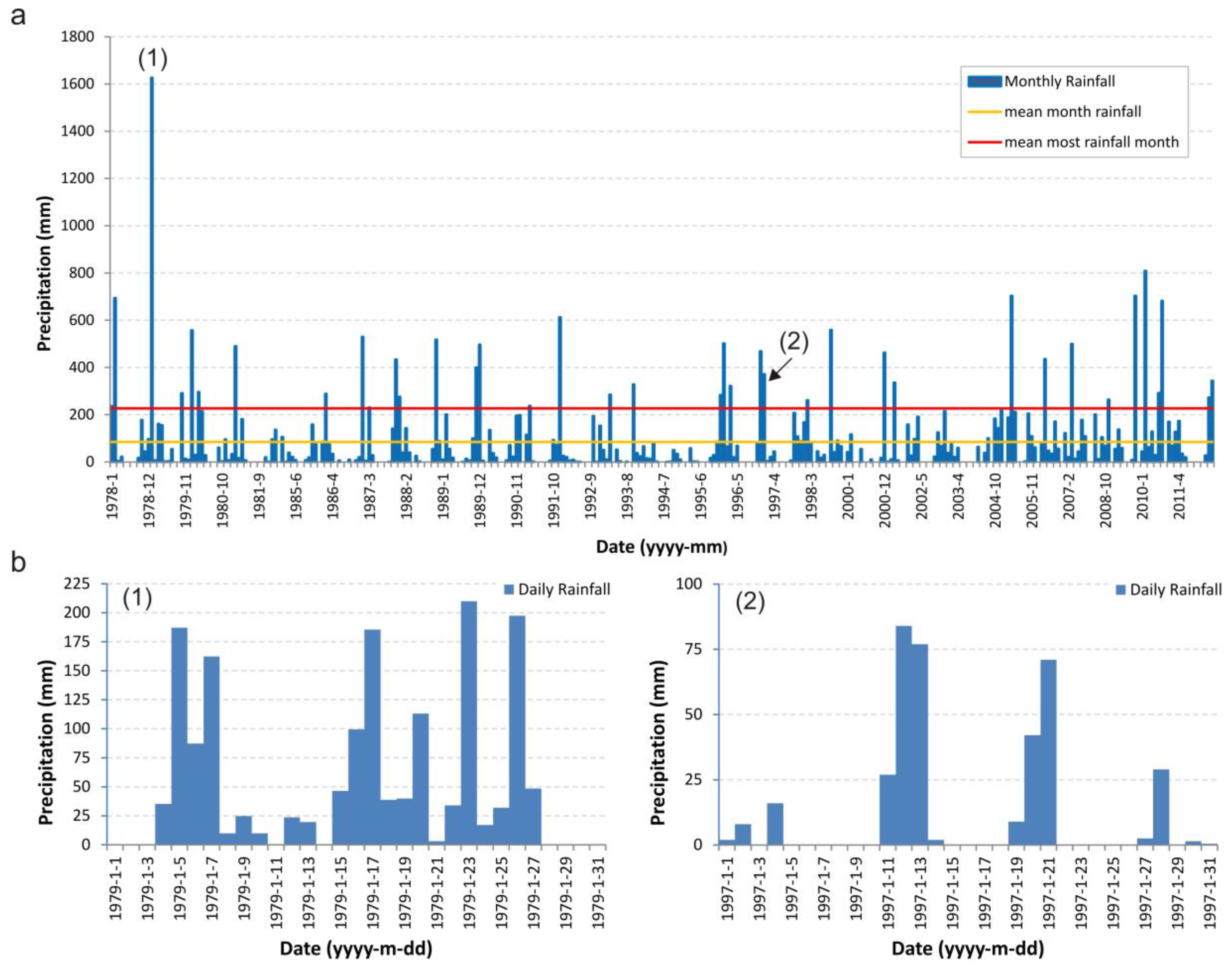
2.2. Precipitation
2.3. Vegetation and Land Use
3. Material and Methods
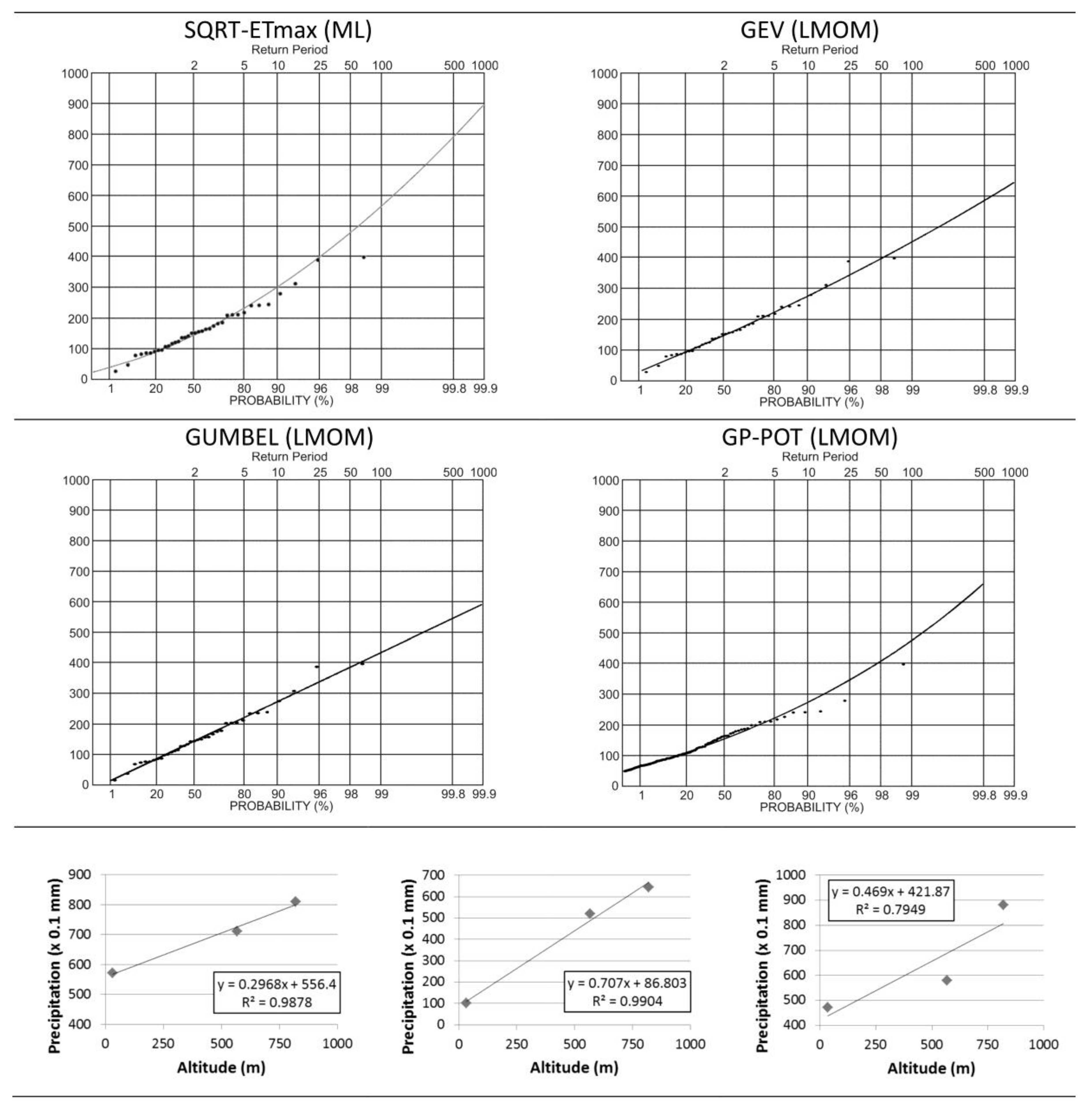
3.1. Precipitation Analysis
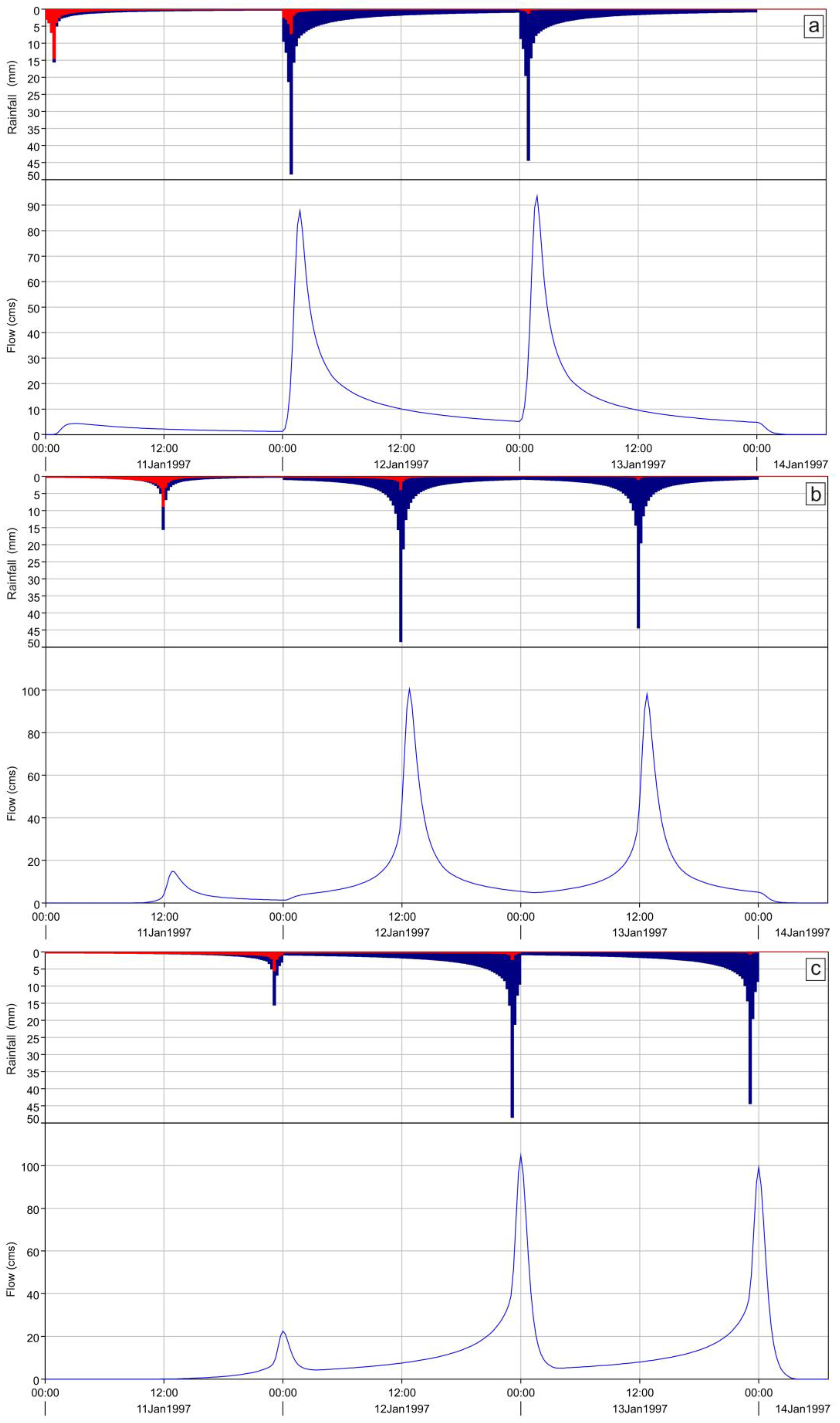
3.2. Rainfall-Runoff Modeling
3.3. Flood Discharge Estimation Using Manning’s Equation
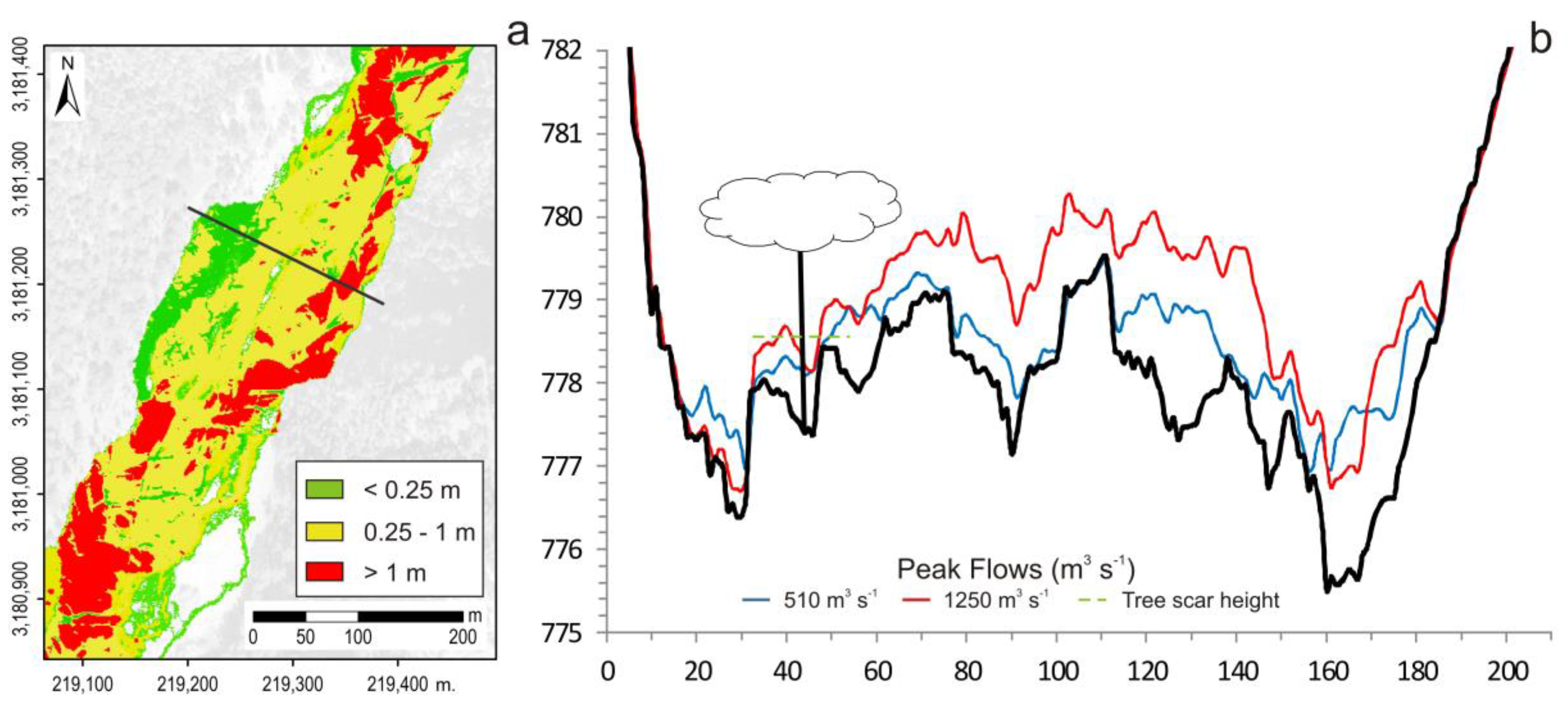
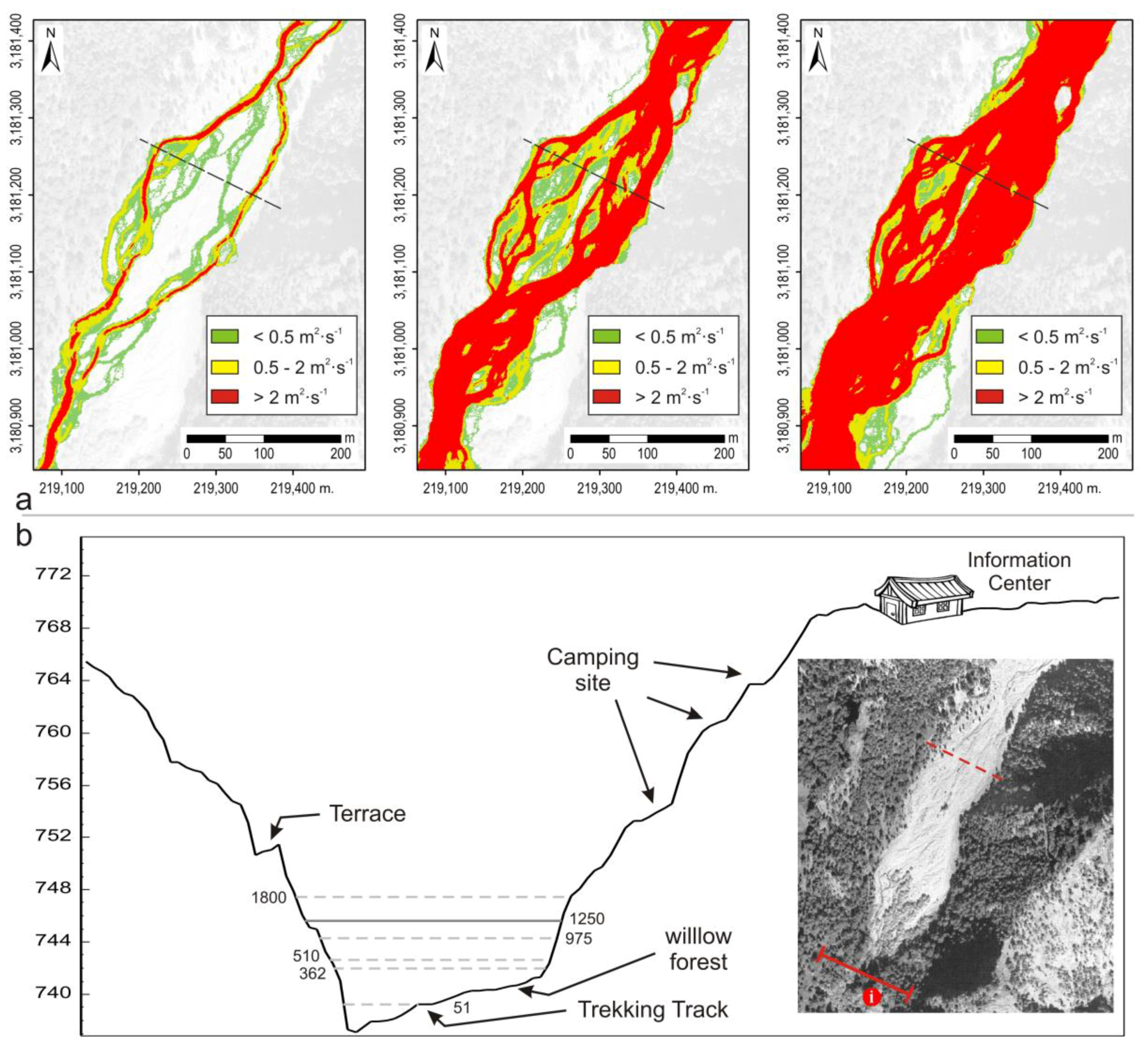
3.4. 2D Hydraulic Modeling
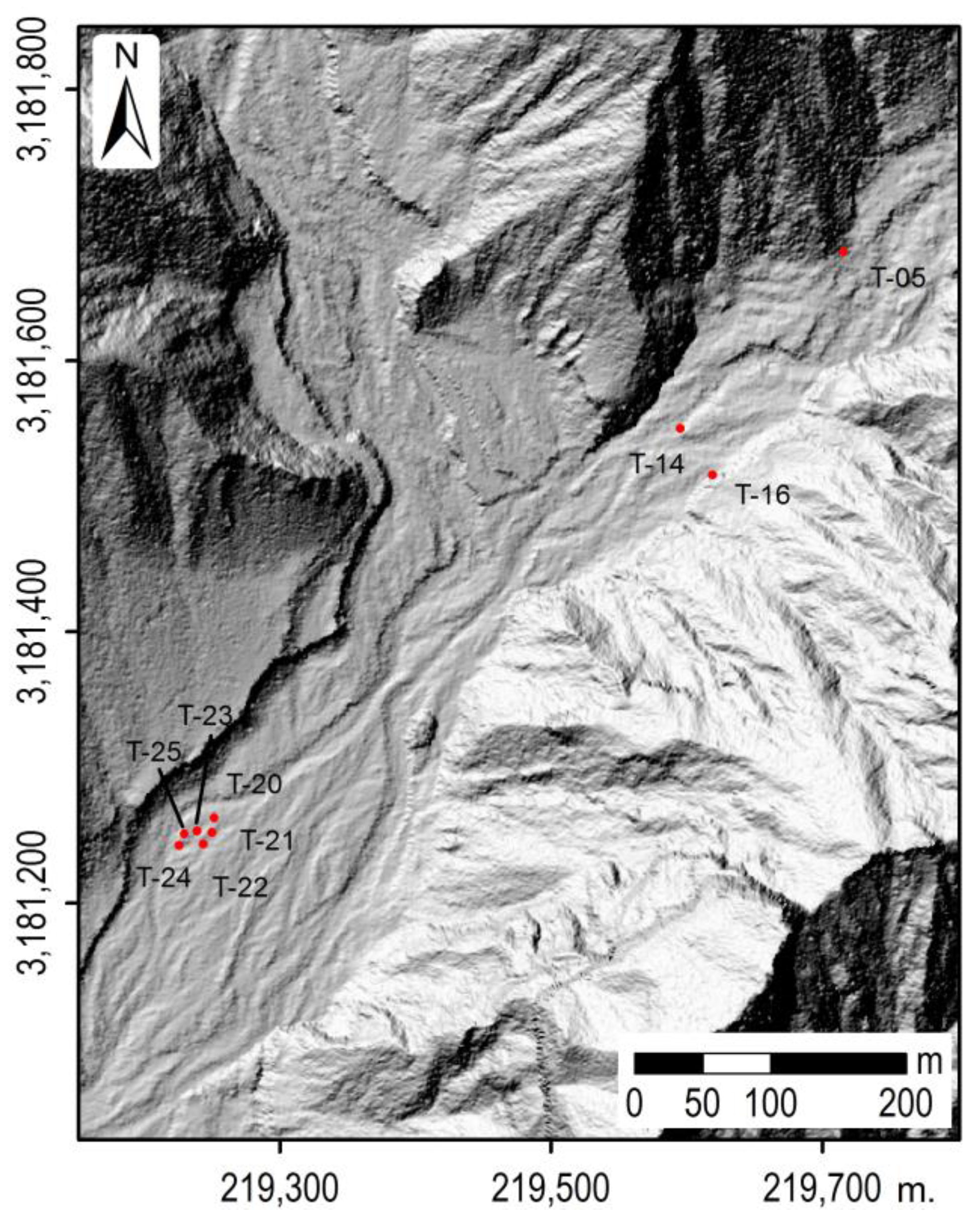
3.5. Dendrogeomorphological Data Sources
4. Results
4.1. Maximum Precipitation Results
4.2. Flood Discharges
4.3. Comparing Results
4.4. Uncertain Sources
5. Discussion
Flooded Areas in Caldera de Taburiente N.P. Past Flood Events
6. Conclusions
- -
- Work undertaken in areas with very scarce availability of systematic information, and disparity in time-space data resolution. Thus, the proposed methodology can be applied to other areas with similar characteristics, a high proportion of drainage basins in mountain areas worldwide (especially outside Europe and the US).
- -
- Different techniques and methods (hydrological, hydraulic, dendro-geomorphological ...) have been combined to make best use of the scarce data available.
- -
- Most attention has been paid to the rainfall data, processed first in a classic statistical frequency analysis of 24 h rainfall data. This rainfall data was subsequently re-processed (duration, altitudinal gradient, hyetograph bias) to generate maximum intensity and volume events.
- -
- Is has been noted the results differences derived from a classical rainfall-runoff process modelling (limited by ungauged fluvial basin site place), and those obtained through the incorporation into the analysis of re-worked rainfall data (looking for maximum rainfall intensity events).
- -
- The incorporation of indirect flood dendro-evidence (FDEs) has been included in peak flow assessment, and to calibrate the results obtained previously from statistical analysis of the rainfall data.
- -
- The peak flow results obtained from the rainfall data processed to maximize intensity are lower than those obtained using FDE, but enable an approximate definition of the flooded area, and therefore the flood hazard area.
- -
- These results show the high variability in estimated discharge and water-stage values in study areas where data is scarce, and how this variability, when transferred to risk assessment, can generate important errors and uncertainties.
Acknowledgments
Author Contributions
Conflicts of Interest
References
- Nakamura, F.; Swanson, F.J.; Wondzell, S.M. Disturbance regimes of stream and riparian systems—A disturbance-cascade perspective. Hydrol. Process. 2000, 14, 2849–2860. [Google Scholar] [CrossRef]
- Viviroli, D.; Weingartner, R.; Messerli, B. Assessing the hydrological significance of the world’s mountains. Mt. Res. Dev. 2003, 23, 32–40. [Google Scholar] [CrossRef]
- Rickenmann, D.; Koschni, A. Sediment loads due to fluvial transport and debris flows during the 2005 flood events in Switzerland. Hydrol. Process. 2010, 24, 993–1007. [Google Scholar] [CrossRef]
- Roe, G.H. Orographic precipitation. Annu. Rev. Earth Planet. Sci. 2005, 33, 645–671. [Google Scholar] [CrossRef]
- Rotunno, R.; Houze, R.A. Lessons on orographic precipitation from the mesoscale alpine programme. Q. J. R. Meteorol. Soc. 2007, 133, 811–830. [Google Scholar] [CrossRef]
- Borga, M.; Boscolo, P.; Zanon, F.; Sangati, M. Hydrometeorological analysis of the 29 August 2003 flash flood in the Eastern Italian Alps. J. Hydrometeorol. 2007, 8, 1049–1067. [Google Scholar] [CrossRef]
- Borga, M.; Gaume, E.; Creutin, J.D.; Marchi, L. Surveying flash floods: Gauging the ungauged extremes. Hydrol. Process. 2008, 22, 3883–3885. [Google Scholar] [CrossRef]
- Seger, M. Landscapes and Living Spaces in the Alps—Between Value Generation and Value Appreciation. Mitt. Osterr. Geogr. G. 2009, 151, 406–407. [Google Scholar]
- White, S.; Garcia-Ruiz, J.M.; Marti, C.; Valero, B.; Errea, M.P.; Gomez-Villar, A. The 1996 Biescas Campsite Disaster in the central Spanish Pyrenees, and its temporal and spatial context. Hydrol. Process. 1997, 11, 1797–1812. [Google Scholar] [CrossRef]
- Benito, G.; Grodek, T.; Enzel, Y. The geomorphic and hydrologic impacts of the catastrophic failure of flood-control-dams during the 1996-Biescas flood (central Pyrenees, Spain). Z. Geomorphol. 1998, 42, 417–437. [Google Scholar]
- Gaume, E.; Borga, M. Post-flood field investigations in upland catchments after major flash floods: Proposal of a methodology and illustrations. J. Flood Risk Manag. 2008, 1, 175–189. [Google Scholar] [CrossRef]
- Benito, G.; Thorndycraft, V.R. Palaeoflood hydrology and its role in applied hydrological sciences. J. Hydrol. 2005, 313, 3–15. [Google Scholar] [CrossRef]
- Gaume, E. On the asymptotic behavior of flood peak distributions. Hydrol. Earth Syst. Sci. 2006, 10, 233–243. [Google Scholar] [CrossRef]
- Omang, R.J.; Parrett, C.; Hull, J.A. Flood Estimates for Ungaged Streams in Glacier and Yellowstone National Parks, Montana; Water-Resources Investigations Report 83-4147; U.S. Geological Survey: Helena, MT, USA, 1983.
- Kresch, D.L. Flood Hazard Assessment of the Hoh River at Olympic National Park Ranger Station, Washington; Water-Resources Investigations Report 86-4198; U.S. Geological Survey: Tacoma, WA, USA, 1987.
- Smillie, G.M.; Ellerbroek, D. Flood Hazard Evaluation for Divide and Wild Creeks Glazier National Park; Technical Report NPS/NR WRD/NRTR-91/02; Bibliogov: Fort Collins, CO, USA, 1991. [Google Scholar]
- Sivapalan, M. Prediction in ungauged basins: A grand challenge for theoretical hydrology. Hydrol. Process. 2003, 17, 3163–3170. [Google Scholar] [CrossRef]
- Hrachowitz, M.; Savenije, H.H.G.; Blöschl, G.; McDonnell, J.J.; Sivapalan, M.; Pomeroy, J.W.; Arheimer, B.; Blume, T.; Clark, M.P.; Ehret, U.; et al. A decade of Predictions in Ungauged Basins (PUB)—A review. Hydrol. Sci. J. 2013, 58, 1198–1255. [Google Scholar] [CrossRef]
- Efstratiadis, A.; Koussis, A.D.; Koutsoyiannis, D.; Mamassis, N. Flood design recipes vs. reality: Can predictions for ungauged basins be trusted? Nat. Hazards Earth Syst. 2014, 14, 1417–1428. [Google Scholar] [CrossRef]
- Biondi, D.; De Luca, D.L. Process-based design flood estimation in ungauged basins by conditioning model parameters on regional hydrological signatures. Nat. Hazards 2015, 79, 1015–1038. [Google Scholar] [CrossRef]
- Colmenero, J.R.; De la Nuez, J.; Casillas, R.; Castillo, C. Epiclastic deposits associated with large-scale landslides and the formation of erosive calderas in oceanic islands: The example of the La Palma Island (Canary Archipelago). Geomorphology 2012, 177, 108–127. [Google Scholar] [CrossRef]
- Staudigel, H.; Féraud, G.; Giannerini, G. The history of intrusive activity on the island of La Palma (Canary Islands). J. Volcanol. Geotherm. Res. 1986, 27, 299–322. [Google Scholar] [CrossRef]
- Ancochea, E.; Hernán, F.; Cendrero, A.; Cantagrel, J.M.; Fuster, J.M.; Ibarrola, E.; Coello, J. Constructive and destructive episodes in the building of a young oceanic island, La Palma, Canary Islands, and genesis of the Caldera de Taburiente. J. Volcanol. Geoth. Res. 1994, 60, 243–262. [Google Scholar] [CrossRef]
- Carracedo, J.C.; Day, S.J.; Guillou, H.; Pérez Torrado, F.J. Giant Quaternary landslides in the evolution of La Palma and El Hierro, Canary Islands. J. Volcanol. Geotherm. Res. 1999, 94, 169–190. [Google Scholar] [CrossRef]
- Marzol, M.V.; Yanes, A.; Romero, C.; Brito de Azevedo, S.; Parada, A.; Martins, A. Los riesgos de las lluvias torrenciales en las islas de la Macaronesia (Azores, Madeira, Canarias y Cabo Verde). In Clima, Sociedad y Medio Ambiente; Cuadrats, J.M., Saz, M.A., Vicente, S.M., Lanjeri, S., De Luis, M., Gonzalez-Hidalgo, J.C., Eds.; Spanish Association of Climatology: Zaragoza, Spain, 2006; pp. 443–452. [Google Scholar]
- Dorta, P. Catálogo de riesgos climáticos en Canarias: Amenazas y vulnerabilidad. Geographicalia 2007, 51, 133–160. [Google Scholar]
- Arco, M.J.; Wildpret, W.; Pérez de Paz, P.L.; Rodríguez, O.; Acebes, J.R.; García, A.; Martín, V.E.; Reyes, A.; Salas, M.; Díaz, M.A.; et al. Mapa de la Vegetación de Canarias; GRAFCAN: Santa Cruz de Tenerife, Spain, 2006. [Google Scholar]
- Garzón-Machado, V.; González-Mancebo, J.M.; Palomares-Martínez, A.; Acevedo-Rodríguez, A.; Fernández-Palacios, J.M.; Del Arco, M.J.; Pérez de Paz, P.L. Strong negative effect of alien herbivores on endemic legumes of the Canary pine forest. Biol. Conserv. 2010, 143, 2685–2694. [Google Scholar] [CrossRef]
- Etoh, T.; Murota, A.; Nakanishi, M. SQRT-Exponential Type Distribution of Maximum. In Hydrologic Frequency Modelling, Proceedings of the International Symposium on Flood Frequency and Risk Analyses, Baton Rouge, LA, USA, 14–17 May 1986; Shing, V.P., Ed.; Reidel Publishing Co.: Boston, MA, USA, 1987; pp. 253–264. [Google Scholar]
- Coles, S. An Introduction to Statistical Modeling of Extreme Values; Springer: London, UK, 2001. [Google Scholar]
- Wang, Q.J. The POT model described by the generalized Pareto distribution with Poisson arrival rate. J. Hydrol. 1991, 129, 263–280. [Google Scholar] [CrossRef]
- Wilks, D.S. Comparison of three-parameter probability distributions for representing annual extreme and partial duration precipitation series. Water Resour. Res. 1993, 29, 3543–3549. [Google Scholar] [CrossRef]
- Coles, S.; Pericchi, L.R.; Sisson, S. A fully probabilistic approach to extreme rainfall modelling. J. Hydrol. 2003, 273, 35–50. [Google Scholar] [CrossRef]
- Cunnane, C. A particular comparison of annual maxima and partial duration series methods of flood frequency prediction. J. Hydrol. 1973, 18, 257–271. [Google Scholar] [CrossRef]
- Madsen, H.; Pearson, C.P.; Rosbjerg, D. Comparison of annual maximum series and partial duration methods for modelling extreme hydrologic events. 1. At-site modelling. Water Resour. Res. 1997, 33, 759–769. [Google Scholar] [CrossRef]
- Salas, L.; Fernandez, J.A. “In-site” regionalization to estimate an intensity-duration-frequency law: A solution to scarce spatial data in Spain. Hydrol. Process. 2007, 21, 3507–3513. [Google Scholar] [CrossRef]
- Chow, V.T.; Maidment, D.R.; Mays, L.W. Hidrología Aplicada; Mc Graw Hill: Bogota, Colombia, 1994. [Google Scholar]
- U.S. Department of Agriculture; Natural Resources Conservation Service. National Engineering Handbook Hydrology Chapters; Chapters 4–10. Available online: https://www.nrcs.usda.gov/wps/portal/nrcs/detailfull/national/water/manage/hydrology/?cid=stelprdb1043063 (accessed on 1 October 2017).
- Boughton, W.C. A review of the USDA SCS Curve Number method. Aust. J. Soil Res. 1989, 27, 511–523. [Google Scholar] [CrossRef]
- Ponce, V.M.; Hawkins, R.H. Runoff Curve Number: Has it reached maturity? J. Hydrol. Eng. 1996, 1, 11–19. [Google Scholar] [CrossRef]
- Adib, A.; Salarijazi, M.; Shooshtari, M.M.; Akhondali, A.M. Comparison between characteristics of geomorphoclimatic instantaneous unit hydrograph be produced by GcIUH based Clark model and Clark IUH model. J. Mar. Sci. Technol. 2011, 19, 201–209. [Google Scholar]
- Rico, M.; Benito, G.; Barnolas, A. Combined palaeoflood and rainfall-runoff assessment of mountain floods (Spanish Pyrenees). J. Hydrol. 2001, 245, 59–72. [Google Scholar] [CrossRef]
- Ponce, V.M.; Yevjevich, V. Muskingum-Cunge method with variable parameters. J. Hydraul. Eng. Div. Am. Soc. Civ. Eng. 1978, 104, 1663–1667. [Google Scholar] [CrossRef]
- Benito, G.; Díez-Herrero, A. Palaeoflood Hydrology: Reconstructing Rare Events and Extreme Flood Discharges. In Hydro-Meteorological Hazards, Risks, and Disasters; Paron, P., Di Baldassarre, G., Eds.; Elsevier: Amsterdam, The Netherlands, 2015; pp. 65–104. [Google Scholar]
- Díez-Herrero, A.; Lain-Huerta, L.; Llorente-Isidro, M. A Handbook on Flood Hazard Mapping Methodologies; Geological Survey of Spain (IGME): Madrid, Spain, 2009. [Google Scholar]
- Arcement, G.J.; Schneider, V.R. Guide for Selecting Manning’s Roughness Coefficients for Natural Channels and Flood Plains; United States Geological Survey (USGS): Denver, FL, USA, 1989.
- Bladé, E.; Cea, L.; Corestein, G.; Escolano, E.; Puertas, J.; Vázquez-Cendón, E.; Dolz, J.; Coll, A. Iber: Herramienta de simulación numérica del flujo en ríos. Revista Internacional de Métodos Numéricos para Cálculo y Diseño en Ingeniería 2014, 30, 1–10. [Google Scholar] [CrossRef]
- Díez-Herrero, A.; Ballesteros, J.A.; Ruiz-Villanueva, V.; Bodoque, J.M. A review of dendrogeomorphological research applied to flood risk analysis in Spain. Geomorphology 2013, 196, 211–220. [Google Scholar] [CrossRef]
- Génova, M.; Ballesteros, J.A.; Mayer, P.; Rubiales, J.M.; Saz, M.A.; Díez-Herrero, A. Multidisciplinary study of flash floods in the Caldera de Taburiente National Park (Canary Islands, Spain). Catena 2015, 131, 22–34. [Google Scholar] [CrossRef]
- Ballesteros-Cánovas, J.A.; Sanchez-Silva, M.; Bodoque, J.M.; Díez-Herrero, A. An Integrated Approach to Flood Risk Management: A Case Study of Navaluenga (Central Spain). Water Resour. Manag. 2013, 27, 3051–3069. [Google Scholar] [CrossRef]
- Ruiz-Villanueva, V.; Bodoque, J.M.; Díez-Herrero, A.; Eguibar, M.A.; Pardo-Igúzquiza, E. Reconstruction of a flash flood with large wood transport and its influence on hazard patterns in an ungauged mountain basin. Hydrol. Process. 2013, 27, 3424–3437. [Google Scholar] [CrossRef]
- Bodoque, J.M.; Eguibar, M.A.; Díez-Herrero, A.; Gutiérrez-Perez, I.; Ruiz-Villanueva, V. Can the discharge of a hyperconcentrated flow be estimated from paleoflood evidence? Water Resour. Res. 2011, 47, W12535. [Google Scholar] [CrossRef]
- Merz, B.; Thieken, A.H. Separating natural and epistemic uncertainty in flood frequency analysis. J. Hydrol. 2005, 309, 114–132. [Google Scholar] [CrossRef]
- Vandewiele, G.L.; Atlabachew, E. Monthly water balance of ungauged catchments obtained by geographical regionalization. J. Hydrol. 1995, 170, 277–291. [Google Scholar] [CrossRef]
- Bárdossy, A. Calibration of hydrological model parameters for ungauged catchments. Hydrol. Earth Syst. Sci. 2007, 11, 703–710. [Google Scholar] [CrossRef]
- Rafiei Emam, A.; Kappas, M.; Hoang Khanh Nguyen, L.; Renchin, T. Hydrological Modeling in an Ungauged Basin of Central Vietnam Using SWAT Model. Hydrol. Earth Syst. Sci. 2016, 2016, 1–33. [Google Scholar] [CrossRef]
- Smith, L.C. Satellite remote sensing of river inundation area, stage, and discharge: A review. Hydrol. Process. 1997, 11, 1427–1439. [Google Scholar] [CrossRef]
- Khan, S.I.; Hong, Y.; Wang, J.; Yilmaz, K.K.; Gourley, J.J.; Adler, R.F.; Brakenridge, G.R.; Policelli, F.; Habib, S.; Irwin, D. Satellite Remote Sensing and Hydrologic Modeling for Flood Inundation Mapping in Lake Victoria Basin: Implications for Hydrologic Prediction in Ungauged Basins. IEEE Trans. Geosci. Remote Sens. 2011, 49, 85–95. [Google Scholar] [CrossRef]
- Knebl, M.R.; Yang, Z.-L.; Hutchison, K.; Maidment, D.R. Regional scale flood modeling using NEXRAD rainfall, GIS, and HEC-HMS/RAS: A case study for the San Antonio River Basin Summer 2002 storm event. J. Environ. Manag. 2005, 75, 325–336. [Google Scholar] [CrossRef] [PubMed]
- Ballesteros-Cánovas, J.A.; Eguibar, M.; Bodoque, J.M.; Díez-Herrero, A.; Stoffel, M.; Gutierrez-Perez, I. Estimating flash flood discharge in an ungauged mountain catchment with 2D hydraulic models and dendrogeomorphic paleostage indicators. Hydrol. Process. 2011, 25, 970–979. [Google Scholar] [CrossRef]
- Ballesteros, J.A.; Bodoque, J.M.; Díez-Herrero, A.; Sanchez-Silva, M.; Stoffel, M. Calibration of floodplain roughness and estimation of flood discharge based on tree-ring evidence and hydraulic modelling. J. Hydrol. 2011, 403, 103–115. [Google Scholar] [CrossRef]
- Ballesteros-Cánovas, J.A.; Stoffel, M.; St George, S.; Hirschboeck, K. A review of flood records from tree rings. Prog. Phys. Geogr. 2015, 39, 1–23. [Google Scholar] [CrossRef]
- Diakakis, M. A method for flood hazard mapping based on basin morphometry: Application in two catchments in Greece. Nat. Hazards 2011, 56, 803–814. [Google Scholar] [CrossRef]
- Karymbalis, E.; Katsafados, P.; Chalkias, C.; Gaki-Papanastassiou, K. An integrated study for the evaluation of natural and anthropogenic causes of flooding in small catchments based on geomorphological and meteorological data and modeling techniques: The case of the Xerias torrent (Corinth, Greece). Z. Geomorphol. 2012, 56, 45–67. [Google Scholar] [CrossRef]
- Abt, S.R.; Wittler, R.J.; Taylor, A.; Love, D.J. Human stability in a high hazard flood zone. JAWRA J. Am. Water Resour. Assoc. 1989, 25, 881–890. [Google Scholar] [CrossRef]
- Merz, B.; Thieken, A.H.; Gocht, M. Flood risk mapping at the local scale: Concepts and challenges. In Flood Risk Management in Europe; Begum, S., Stive, M.J.F., Hall, J.W., Eds.; Springer: Dordrecht, The Netherlands, 2007; pp. 231–251. [Google Scholar]


| 24 h Rainfall Events | ||||||||
|---|---|---|---|---|---|---|---|---|
| T (year) | p (T) | SQRT ML 1 | GEV LMOM 1 | GEV ML 1 | Gumbel LMOM 1 | Gumbel ML 1 | GP-POT LMOM 2 | Mean Value |
| 2 | 0.5 | 145 | 147 | 150 | 150 | 150 | 156 | 150 |
| 5 | 0.8 | 234 | 224 | 224 | 226 | 224 | 224 | 226 |
| 10 | 0.9 | 304 | 277 | 273 | 277 | 272 | 275 | 280 |
| 25 | 0.96 | 402 | 346 | 337 | 341 | 334 | 349 | 352 |
| 50 | 0.98 | 482 | 400 | 384 | 388 | 380 | 411 | 408 |
| 100 | 0.99 | 569 | 455 | 432 | 435 | 425 | 480 | 466 |
| 200 | 0.995 | 662 | 512 | 480 | 482 | 470 | 551 | 526 |
| 500 | 0.998 | 793 | 590 | 544 | 544 | 530 | 660 | 610 |
| K-S Test | 0.0811 | 0.0541 | 0.0541 | 0.0811 | 0.0541 | 0.0336 | ||
| Mean Error | 0.0808 | 0.0494 | 0.0490 | 0.0435 | 0.0490 | 0.0191 | ||
| R2 | 0.9893 | 0.9950 | 0.9951 | 0.9943 | 0.9949 | 0.9944 | ||
| Rainfall Event Models | Maximum Hourly Rainfall Intensity (mm h−1) |
|---|---|
| 11–13 January 1997. C106U station rainfall. 72 h (27 + 87 + 77 mm) hyetograph (Right Skewed) | 14 |
| C106U T2 rainfall (GP-POT). 24 h hyetograph | 21 |
| C106U T5 rainfall (GP-POT). 24 h hyetograph | 30 |
| C106U T10 rainfall (GP-POT). 24 h hyetograph | 36 |
| C106U T25 rainfall (GP-POT). 24 h hyetograph | 46 |
| C106U T50 rainfall (GP-POT). 24 h hyetograph | 54 |
| C106U T100 rainfall (GP-POT). 24 h hyetograph | 63 |
| C106U T200 rainfall (GP-POT). 24 h hyetograph | 73 |
| C106U T500 rainfall (GP-POT). 24 h hyetograph | 87 |
| 19–20 January 1997. C106U station rainfall. 1 h hyetograph. | 176 |
| C106U T2 rainfall (mean value). 1 h hyetograph | 150 |
| C106U T5 rainfall (mean value). 1 h hyetograph | 226 |
| C106U T10 rainfall (mean value). 1 h hyetograph | 280 |
| C106U T25 rainfall (mean value). 1 h hyetograph | 352 |
| C106U T50 rainfall (mean value). 1 h hyetograph | 408 |
| C106U T100 rainfall (mean value). 1 h hyetograph | 466 |
| C106U T200 rainfall (mean value). 1 h hyetograph | 526 |
| C106U T500 rainfall (mean value). 1 h hyetograph | 610 |
| 19–20 January 1997. C106U station rainfall. Rainfall—Elevation gradient (0.071 mm m−1). 1 h hyetograph. | 236 |
| Rainfall-Runoff Event Models | “Verduras de Alfonso” Ravine | “Cantos de Turugumay” Ravine | “Playa de Taburiente” Outflow Point |
|---|---|---|---|
| 11–13 January 1997. C106U station rainfall. 72 h (27 + 87 + 77 mm) hyetograph (Right Skewed) | 19 | 25 | 51 |
| 11–13 January 1997. C106U station rainfall. 72 h (27 + 87 + 77 mm) hyetograph (RS). CN + 10% | 20 | 27 | 54 |
| 11–13 January 1997. C106U station rainfall. 72 h (27 + 87 + 77 mm) hyetograph (RS). CN + 25% | 23 | 30 | 60 |
| C106U T2 rainfall (GP-POT). 24 h hyetograph | 35 | 47 | 95 |
| C106U T5 rainfall (GP-POT). 24 h hyetograph | 57 | 74 | 152 |
| C106U T10 rainfall (GP-POT). 24 h hyetograph | 73 | 94 | 194 |
| C106U T25 rainfall (GP-POT). 24 h hyetograph | 95 | 123 | 255 |
| C106U T50 rainfall (GP-POT). 24 h hyetograph | 114 | 147 | 306 |
| C106U T100 rainfall (GP-POT). 24 h hyetograph | 136 | 174 | 362 |
| C106U T200 rainfall (GP-POT). 24 h hyetograph | 157 | 202 | 420 |
| C106U T500 rainfall (GP-POT). 24 h hyetograph | 190 | 244 | 509 |
| 19–20 January 1997. C106U station rainfall. 1 h (176 mm) hyetograph. | 65 | 94 | 180 |
| 19–20 January 1997. C106U station rainfall. 1 h (176 mm) hyetograph. CN + 10% | 78 | 111 | 216 |
| 19–20 January 1997. C106U station rainfall. 1 h (176 mm) hyetograph. CN + 25% | 98 | 135 | 268 |
| C106U T2 rainfall (mean value). 1 h hyetograph | 49 | 73 | 137 |
| C106U T5 rainfall (mean value). 1 h hyetograph | 95 | 134 | 264 |
| C106U T10 rainfall (mean value). 1 h hyetograph | 130 | 179 | 358 |
| C106U T25 rainfall (mean value). 1 h hyetograph | 178 | 242 | 489 |
| C106U T50 rainfall (mean value). 1 h hyetograph | 216 | 290 | 592 |
| C106U T100 rainfall (mean value). 1 h hyetograph | 256 | 342 | 702 |
| C106U T200 rainfall (mean value). 1 h hyetograph | 297 | 395 | 815 |
| C106U T500 rainfall (mean value). 1 h hyetograph | 357 | 470 | 975 |
| 19–20 January 1997. C106U station rainfall. Rainfall—Elevation gradient (0.071 mm/m). 1 h (236 mm) hyetograph. | 100 | 143 | 265 |
| 19–20 January 1997. C106U station rainfall. Rainfall—Elevation gradient (0.071 mm/m). 1 h (236 mm) hyetograph. CN + 10% | 116 | 162 | 306 |
| 19–20 January 1997. C106U station rainfall. Rainfall—Elevation gradient (0.071 mm/m). 1 h (236 mm) hyetograph. CN + 25% | 138 | 187 | 362 |
| Peak flows that minimize RMSE for dendro-geomorphological evidences. | - | - | ~1250 |
| Tree Sample | Peak Flow (m3 s−1) | Mean Peak Flow (m3 s−1) | |
|---|---|---|---|
| T-05 | 2416 | - | 1798 (629) |
| T-14 | 780 | - | |
| T-16 | 2162 | - | |
| T-20 | 2574 | 1804 (569) | |
| T-21 | 2210 | ||
| T-22 | 928 | ||
| T-23 | 1765 | ||
| T-24 | 1504 | ||
| T-25 | 1845 | ||
© 2017 by the authors. Licensee MDPI, Basel, Switzerland. This article is an open access article distributed under the terms and conditions of the Creative Commons Attribution (CC BY) license (http://creativecommons.org/licenses/by/4.0/).
Share and Cite
Garrote, J.; Díez-Herrero, A.; Bodoque, J.M.; Perucha, M.A.; Mayer, P.L.; Génova, M. Flood Hazard Management in Public Mountain Recreation Areas vs. Ungauged Fluvial Basins. Case Study of the Caldera de Taburiente National Park, Canary Islands (Spain). Geosciences 2018, 8, 6. https://doi.org/10.3390/geosciences8010006
Garrote J, Díez-Herrero A, Bodoque JM, Perucha MA, Mayer PL, Génova M. Flood Hazard Management in Public Mountain Recreation Areas vs. Ungauged Fluvial Basins. Case Study of the Caldera de Taburiente National Park, Canary Islands (Spain). Geosciences. 2018; 8(1):6. https://doi.org/10.3390/geosciences8010006
Chicago/Turabian StyleGarrote, Julio, Andrés Díez-Herrero, José M. Bodoque, María A. Perucha, Pablo L. Mayer, and Mar Génova. 2018. "Flood Hazard Management in Public Mountain Recreation Areas vs. Ungauged Fluvial Basins. Case Study of the Caldera de Taburiente National Park, Canary Islands (Spain)" Geosciences 8, no. 1: 6. https://doi.org/10.3390/geosciences8010006