Article

The Study of Geological Structures in Suli and Tulehu Geothermal Regions (Ambon, Indonesia) Based on Gravity Gradient Tensor Data Simulation and Analytic Signal

1
Department of Physics, Faculty of Mathematics and Natural Sciences, Universitas Papua; Papua Barat, Manokwari 98314, Indonesia
2
Department of Physics, Faculty of Mathematics and Natural Sciences, Universitas Gadjah Mada, Yogyakarta 55281, Indonesia
3
Department of Geological Engineering, Faculty of Engineering, Universitas Gadjah Mada, Yogyakarta 55281, Indonesia
*
Author to whom correspondence should be addressed.
Geosciences 2018, 8(1), 4; https://doi.org/10.3390/geosciences8010004
Submission received: 3 October 2017 / Revised: 8 December 2017 / Accepted: 21 December 2017 / Published: 27 December 2017

Abstract

:
In early 2017, the geothermal system in the Suli and Tulehu areas of Ambon (Indonesia) was investigated using a gravity gradient tensor and analytic signal. The gravity gradient tensor and analytic signal were obtained through forward modeling based on a rectangular prism. It was applied to complete Bouguer anomaly data over the study area by using Fast Fourier Transform (FFT). The analysis was conducted to enhance the geological structure like faults as a pathway of geothermal fluid circulation that is not visible on the surface because it is covered by sediment. The complete Bouguer anomaly ranges of 93 mGal up to 105 mGal decrease from the southwest in Suli to the northeast in Tulehu. A high gravity anomaly indicates a strong magmatic intrusion below the Suli region. The gravity anomalies decrease occurs in the Eriwakang mountain and most of Tulehu, and it is associated with a coral limestone. The lower gravity anomalies are located in the north to the northeast part of Tulehu are associated with alluvium. The residual anomaly shows that the drill well TLU-01 and geothermal manifestations along with the Banda, and Banda-Hatuasa faults are associated with lowest gravity anomaly (negative zone). The gravity gradient tensor simulation and an analytic signal of Suli and Tulehu give more detailed information about the geological features. The gzz component allows accurate description of the shape structures, especially the Banda fault associated with a zero value. This result will be useful as a geophysical constraint to subsurface modeling according to gravity gradient inversion over the area.

1. Introduction

Maluku Province, especially Ambon Island (Indonesia), has a geothermal potential that can be developed as alternative energy resources [1]. Ambon Island is a part of the deep Banda arc system with hills characteristics. These hills were formed by the volcanic activity at the end of Pliocene to the earlier of Pleistocene and were dominated by tectonic activity in the form of active faults. Ambon Island is composed of volcanic rock and carbonate sedimentary rocks [1]. Based on a report from the Geological Agency of Indonesia, the largest energy accumulation in the geothermal potential of Ambon Island is located in Suli and Tulehu, with an estimated potential energy of 100 Mwe [2]. Suli and Tulehu geothermal areas are located in the eastern part of Ambon, at an altitude of 76 m above sea level over an area of approximately 21 km2 [3]. Geothermal manifestations in these areas are mostly hot springs, fumarole and alteration rocks associated with the Banda fault. These manifestations appear along the Huwe fault, Tulehu fault, and the Banda fault. Faults and fractures play an important role in the localization and evolution of hydrothermal systems. Hydrothermal activity is highly dependent on the interaction between heat sources, fluid circulation from the subsurface, and permeable layer pathways [4]. However, often these faults and fractures’ structures are not visible at the surface, as they are hidden by younger cover sedimentary rocks, thus making them difficult to detect and map.
Several previous studies have been conducted to learn the geothermal systems in Suli and Tulehu, one of which was the geophysical study, which used the Magnetotelluric (MT) method [1,3,5]. The results of MT inversion showed the 3D preliminary model of subsurface over the study area based on conductivity and resistivity variation of the rock layers. In the Suli and Tulehu areas, there is one geothermal exploration drill hole with shallow cores of about 150 m depth and deeper drill cutting until 930 m depth. However, more information is needed to obtain the comprehensive and more accurate model of the geological structure over the study area for the development of geothermal drilling. In this paper, we used the gravity method to learn about the geothermal system in Suli and Tuhelu. The study of gravity in various places of the world shows very useful results in geothermal exploration, such as delineating fault and fracture zones associated with geothermal reservoir systems [6,7,8]. Gravity field anomaly and its gravity gradients provide important information to delineate geological structures related to economic interests [9].
The conventional gravity measurements show the magnitude of the earth’s gravity field but are less sensitive to determining the boundaries and directions of the anomalies’ objects. The gravity gradient measures show the gradient of spatial rate change of the earth’s gravity field, which is a vector quantity with both magnitude and direction [10]. Other advantages of gravity gradient include high-resolution imaging of the target with a depth of approximately 10 km, and it can detect the edge effects of fault as a geothermal controller, better determining the geological boundaries of anomalies’ objects and other structures [10].
In this research, we performed a forward modeling simulation and fast Fourier transform (FFT) analysis to calculate gravity gradient tensor and an analytic signal from ground gravity data in Suli and Tulehu areas. As direct measurement of gravity gradient tensor will not be feasible, the forward modeling was performed based on a simple 3D rectangular prism as the testing model to calculate the gravity response, its gradients, and analytic signal. In the Fourier domain, the gravity gradient is equal to the multiplication of the gravity with the wave number along with the direction of the derivatives [11,12]. Finally, the results of gravity gradient tensor and an analytic signal of complete Bouguer anomaly in Suli and Tulehu were used to understand, delineate, and determine the relationship between geological structures and geothermal manifestation.

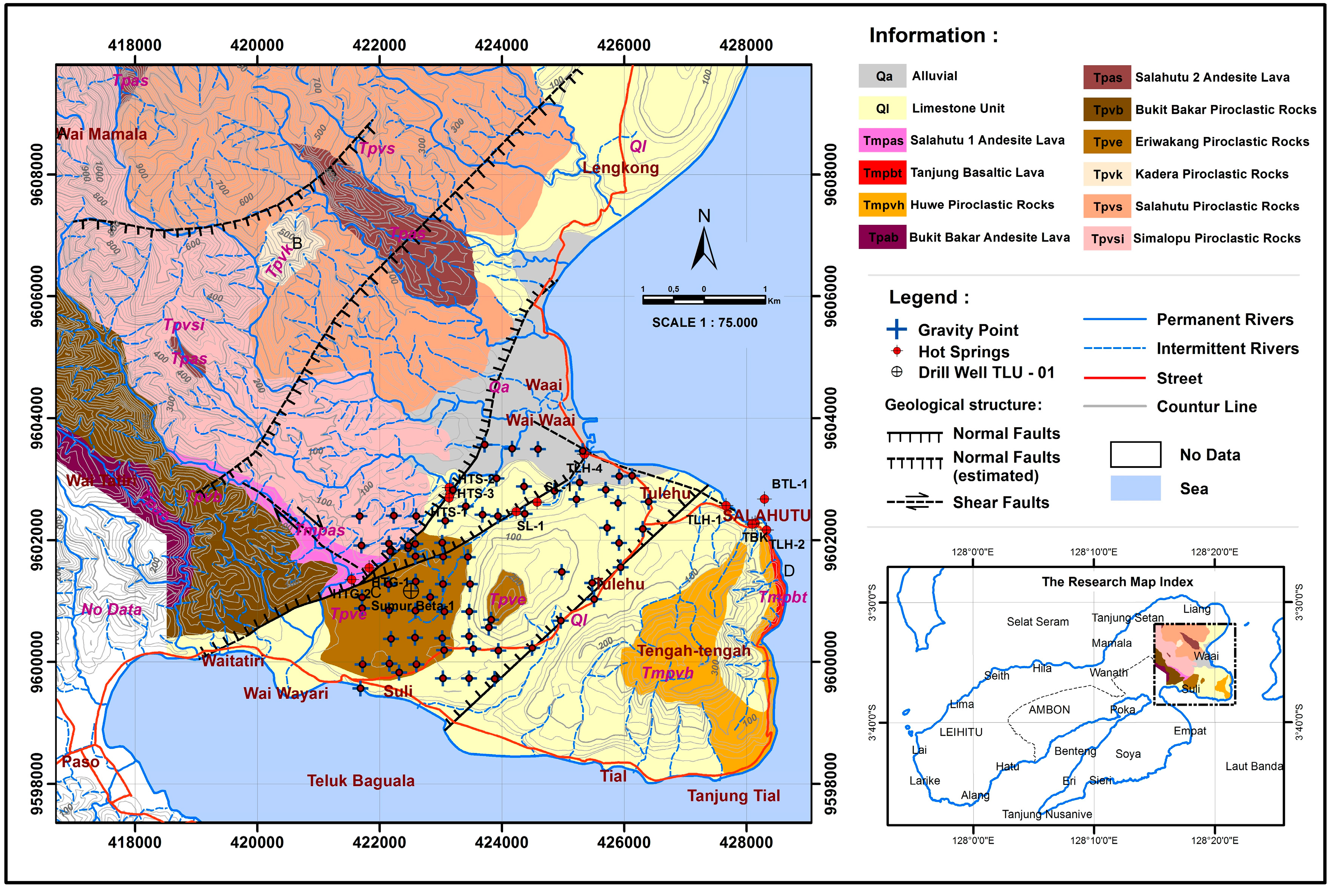
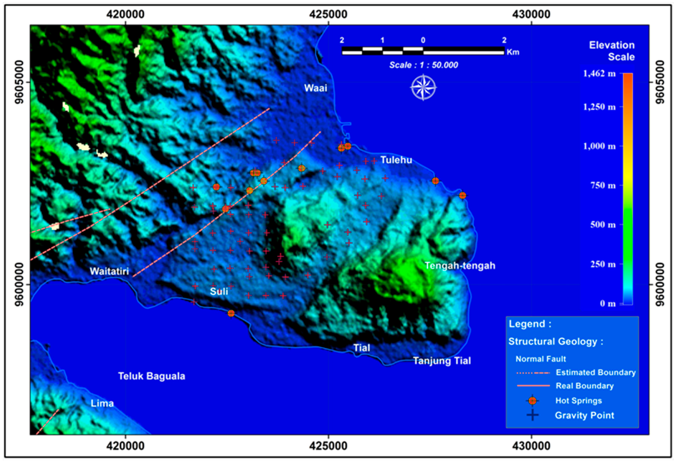
2. Geologic Settings

Eastern Indonesia is one of the most dynamic regions in Indonesia due to the interaction between the three major plates, namely Eurasian, Pacific, and Indo-Australian plates. The Banda arc is the result of such interaction. The southern part of the Banda arc is the interactions between the Eurasian plate and the Indo-Australian plate, while the northern part of the Banda arc is the interactions between the Eurasian plate, the Pacific, and the Indo-Australian [13]. The Banda arc is one of the active arcs as a result of subduction of island arcs and continental crusts. The main geological feature of the Banda arc consists of a deep volcanic arc and non-volcanic outer arc formed of sedimentary rocks, metamorphic rocks, and some igneous rocks mainly from Permian to Quaternary age.
The inner volcanic arc has been active since the late Miocene. The non-volcanic outer arc is widely regarded as a recent zone of collision between the Australian margin and Banda volcanic arc and includes thrust sheets, especially of the Australian sedimentary rocks, but is related to places with some igneous and metamorphic rocks, which have been elevated above the sea level very rapidly since the Middle Pliocene [14,15].
Part of the Banda arc, Ambon Island consists of two distinct geological parts. The first is Hitu in the north and the second is Leitimor in the south [16]. Both are connected by a narrow precarious land. The Hitu region has the main volcanic geological features composed of two major volcanoes at 1038 m and 930 m altitude, mostly composed of cordierite bearing dacites (‘ambonites’). This volcanic type is locally covered by coral reef deposits and Quaternary alluvium at the bottom of the island. Leitimor in the southern part of Ambon is mostly made up of Upper Triassic greywackes and metamorphic limestones tectonically overlain by ophiolitic rocks [16,17].
Based on the Ambon regional geological maps, the lithology of the Suli and Tulehu geothermal area is dominated by Ambon volcanic rocks, composed of andesite lava, dacite, breccia, and tuff lava. Suli and Tulehu are geothermal areas that are approximately 21 km2. Volcanic rocks consist of Tanjung basaltic lava, Huwe pyroclastic rock, Salahutu 1 andesite lava, Salahutu 2 andesite lava, Simalopu pyroclastic rock, Salahutu pyroclastic rock, Kadera pyroclastic rock, Bukitbakar andesite lava, and Eriwakang pyroclastic rock.
Geothermal manifestations in the Suli and Tulehu areas are mostly dominated by hot springs, but also have a fumarole and alteration rock associated with Banda fault. These manifestations occur in the Huwe fault, the Tulehu fault, and the Banda-Hatuasa fault. Fluids on these manifestations have a pH ranging from 5.9 to 8.3 [1,18].
There are three types of hydrothermal fluids in the Suli and Tulehu geothermal areas, namely calcium-bicarbonate, sodium-chloride, and sodium-chloride bicarbonate. These three types of fluids indicate mixing between fluids derived from deep and high-fueled reservoirs with shallow groundwater [1,3]. For the Suli and Tulehu geothermal regions, fault types are the shear dextral faults and the normal faults (down). In this area, there is one geothermal drill well (TLU-01) and seven geothermal manifestations in the form the hot springs. The geological and geothermal manifestation maps in the Suli and Tulehu geothermal regions are shown in Figure 1.

3. Methods

3.1. Gravity Method

The gravity survey was conducted for nine days from 16 February to 25 February 2017. Measurement of the earth’s gravitational field using the gravity meter Lacoste and Romberg model G-1118 Maximum Voltage Retroaction (MVR) feedback system that has a precision of 0.005 mGal. Gravity station elevation measurements using a GPS Trimble navigation 4600 LS single frequency geodetic surveyor (Trimble, Sunnyvale, CA, USA). The data collection was started with a preliminary survey to obtain the position of geothermal manifestations and gravity measurement stations. Based on the preliminary survey, gravity field data measurements were performed on 70 gravity stations with the distance between measuring stations varying from 200 m to 400 m. The measurement was carried out at a topographic range from 5 m to 190 m. The distance depends on an ease of access to the terrain. The location of a geothermal manifestation and the distribution of gravity station were shown in Figure 2.
The gravity field measurement over the study area was done by a looping technique, which it starts at the local gravity and GPS base station (Figure 3a,b), and is then measured station to station, and finally back to the base station on the same day (Figure 3c). The local gravity base station is placed in the office of Suli village. The purpose of this technique is to obtain the drift value caused by the change of gravity meter reading due to the disturbance in the form of an appliance shock, temperature change, and tool fatigue during measurement. In this study, the regional base station of the earth gravity field as an absolute reference point is located in the office of Volcanology and Geological Hazard Mitigation (PVMBG) Yogyakarta, Indonesia. This is because Ambon Island has no absolute reference point. The regional gravity value at the base station in Yogyakarta is 978,202.98 mGal. We make a new reference point in Suli based on the sum of an absolute reference point in Yogyakarta and the different reading of gravity meter in Suli and Yogyakarta. The gravity meter reading is done by five times at each gravity station. To make a complete Bouguer anomaly, the gravity data were corrected for tide, latitude, free air, Bouguer, and terrain effects by using Geosoft Oasis Montaj software (Geosoft, Toronto, ON, Canada).
The latitude correction was performed using the spheroid references with the WGS 1984 formula. The latitude of Suli and Tulehu ranges from 3°35′12″ S to 3°37′21″ S. Geodetic Reference System (GRS) 1980 was used a formula for free air correction with the elevation data from GPS measurement. Then, for Bouguer and terrain corrections, we used an assumed density of 2.673 gr/cm3. It was derived from a Parasnis approach. Terrain correction was calculated using the 50 m mesh digital elevation model of Ambon Island.

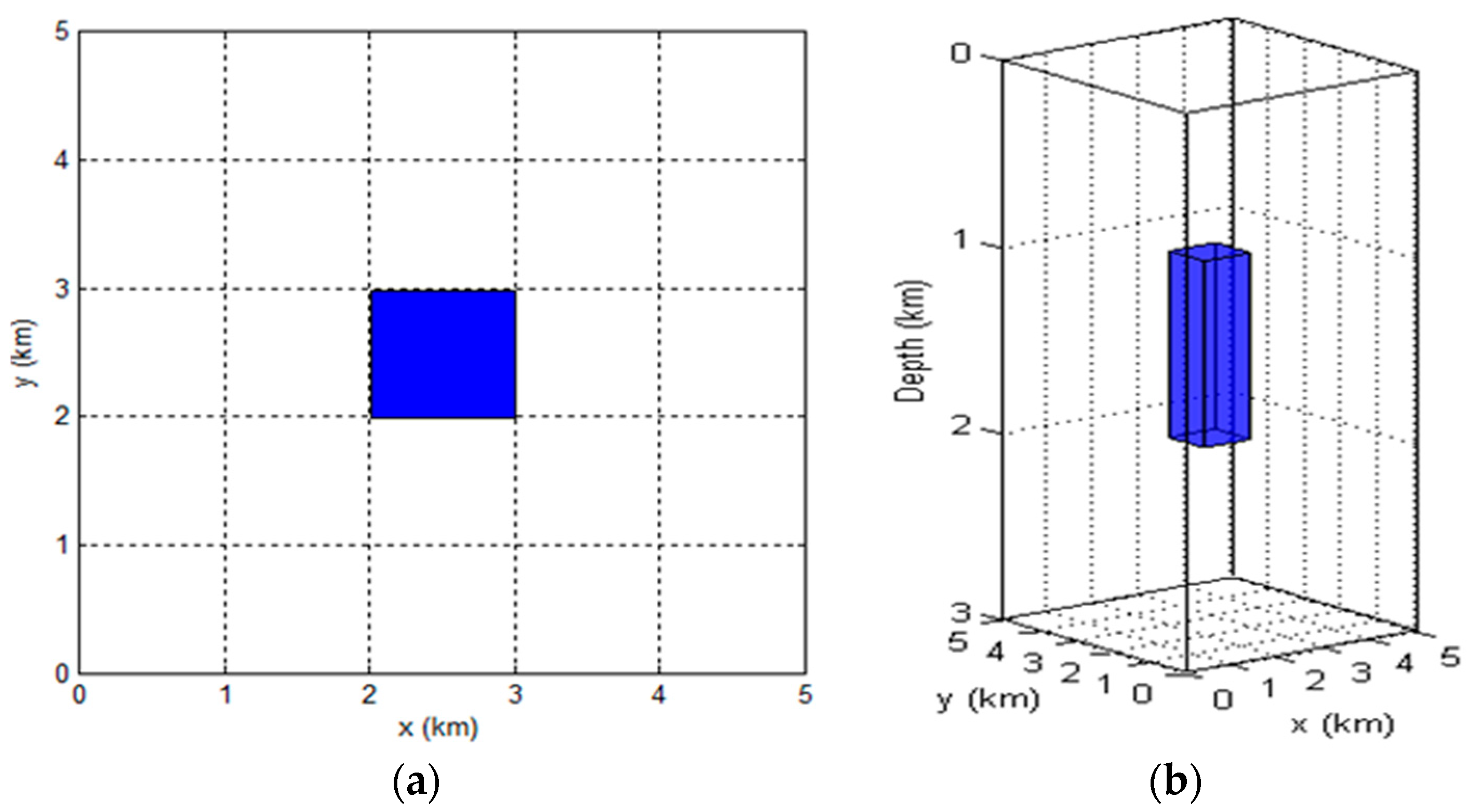
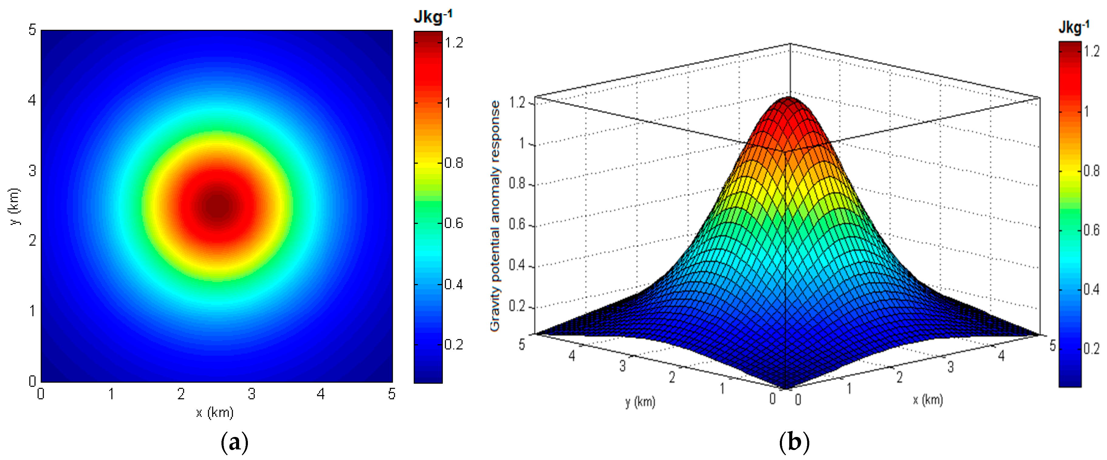
3.2. Calculation of Gravity Gradient Tensor Based on Synthetic Model

The gravity gradient in the international unit system (SI) has a unit of measurement that is m/s2/m = 1/s2 = s−2, or commonly called as Eotvos (E), where 1E = 10−9 s−2. The standard vertical gravity gradient near the surface approaches 3086 E [19]. The usefulness of the gravity gradient in exploration has become important in recent years with the development of airborne gradiometry with an accuracy of ±2–5 Eotvos (1E = 0.1 mGal/km), which has a wavelength that approaches 45 m and 100 km for gradiometer measurements via satellite.
The earth’s gravity potential U of the excess mass distribution with the density ρ on volume V can be written as [20]:
U ( r ) = G V ρ ( r ) | r r | d V ,
where r and r′ denote the observation point and the integral respectively, and G is the earth’s gravitational constant. The gravity gradient tensor can be written as follows:
Γ g = [ 2 U x 2 2 U x y 2 U x z 2 U x y 2 U y 2 2 U y z 2 U x z 2 U y z 2 U z 2 ] = [ g x x g x y g x z g y x g y y g y z g z x g z y g z z ] = [ g x x g x y g x z g x y g y y g y z g x z g y z g z z ] .
The potential of gravity U satisfies the Laplace equation 2 U ( r ) = 0 , and hence there is a zero tensor component. Since Γ g is symmetry, there are only six free tensor components. In the last two decades, the processing and interpretation of gravity gradient tensor data have made significant progress [20].
The complete gravity gradient tensor measurement of the gravitational field is generally carried out by air and satellite measurement, but the gravity gradient tensor can also be calculated from the vertical components of gravity measurements on the ground [11]. In gravity and magnetic surveys, spatial gradients (horizontal and vertical) for potential field data are likely to enhance small or local scale anomalies directly related to anomalous sources. The gravity gradient given directional emphasizes the short wavelength spatial component of gravity anomalies. On the other hand, gravity gradient is often used in interpretations for isolated gravity anomalies. Then, the analytic signal was applied to gravity anomaly data in order to delineate the border, contact, and shape of geological boundaries [21]. In geothermal studies, the measurement and analysis of gravity gradients can provide more benefits when compared to conventional gravity field measurements.
The gravity gradient tensor elements were calculated from the ground measurement of a vertical component using the Fourier transform [11]. In the Fourier domain, the gravity gradient is equal to the multiplication of gravity and the wave number along with the direction of the derivatives [12]. By considering the symmetry of the tensor component and the derived property of the Fourier transform, we can show the Fourier transform as follows [11,12]:
g z y = g y z       i k y G z = | k | G y ,
g x z = g z x       | k | G x = i k x G z ,
g y x = g x y       i k x G y = i k y G x .
Gy(kx,ky) and Gz(kx,ky) and Gz(kx,ky) are the gravity component of Fourier transform of gx, gy, dan gz, while kx and ky are the wave numbers following the equation:
| k | = k x 2 + k y 2 = i k z .
In a conventional gravitational field survey, the measurement values are only on the vertical component (gz). However, the relationship of the horizontal components gx and gy with the vertical component gz of the gravitational field in the Fourier domain is obtained from the relationship of Equations (3a)–(3c), thus:
g x     G x = i k x | k | G z ,
g y     G y = i k y | k | G z .
Therefore, the gravity gradient tensor components can be the theoretical calculation of the gravity measurement anomaly, following the equation:
Δ g = [ Δ g i j ] = F 1 ( [ k x 2 | k | k x k y | k | i k x k x k y | k | k y 2 | k | i k y i k x i k y | k | ] ) .
F−1 is inverse Fourier transform. Equation (6) shows that the gradient calculation can be shown in the Fourier domain as the multiplication of the input signal with the filter function.

3.3. The 3D Analytic Signal of Gravity Data

3.3.1. Forward Modeling of Gravity Gradient Tensor Based on Rectangular Prism

We used Potensoft software (Department of Geophysical Engineering, Faculty of Engineering, Ankara University, Ankara, Turkey) [22] to construct a synthetic model of a 3D rectangular prism. The block model was made for 1 km3 in the x-, y-, and z-directions, located at a depth of 1 km from the surface. The density contrast of the model is 0.43 g/cm3 at the center of an area with 5 km × 5 km (Figure 4). The calculation of theoretical gravity anomaly has been done with a grid of 0.1 km × 0.1 km (Figure 5).
For our testing model, the result of theoretical response is a positive value with a range from 0.075 mGal to 1.24 mGal. The pattern of an anomaly is circular with the highest value at the centre of the circle like that shown in Figure 5.
To obtain the gravity gradient tensor component, the theoretical response of gravity potential anomaly is first described in the form of a derivative into a gravity component in the x-, y-, and z-directions in the Cartesian coordinate system. The derivatives include horizontal (x dan y) and vertical (z) derivative. Horizontal derivatives of gravity potential anomaly are computed in the spatial domain by a central difference approach of finite difference. On the other hand, vertical derivatives process is performed in the frequency domain using fast Fourier transform [22,23]. The gravity field anomaly in the x-, y-, and z-directions is called gx, gy, and gz, as shown in Figure 6. The gravity field anomaly component in x- and y-directions has a negative to positive anomaly value with a range from −0.704 mGal to 0.704 mGal. Those components have a different anomaly pattern. The anomaly component in the x-direction forms the east–west pole pattern with the north–south anomaly boundary. The anomaly component in the y-direction forms a north–south pole pattern with the east–west anomaly boundary. The gravity component in the z-direction has a circular pattern with a negative to positive anomaly value with a range between −0.03 mGal to 1.60 mGal.
Furthermore, the derivative of gravity components in x-, y-, and z-directions produces nine tensor components of gravity gradient. The gravity gradient responses for each of the free tensor components of (gxx, gxy, gxz, gyy, gyz, and gzz) are shown in Figure 7. Based on a rectangular prism, the gravity gradient tensor components have relatively small values ranging from negative to positive and differ in value from one component to another. The anomalies produced by each gravity gradient tensor component have a specific pattern. The gxx component indicates the east and west border of the prism. The gxy component provides information about the four corners and the location of the midpoint of the rectangular prism. The gxz component divides the rectangular prism symmetrically on the east–west and shows the center axis of the north–south. The gyy (Table 1) component indicates the northern and southern borders of the prism. The gyz component divides the rectangular prism symmetrically on the north–south and shows the middle axis of the anomaly to the east–west. The gzz component provides an estimate of the maximum depth and predicts the boundary information that is directly related to the prism anomaly object.
The gravity gradient tensor calculation base on a rectangular prism model produces similar anomaly patterns with some related studies [9,11].

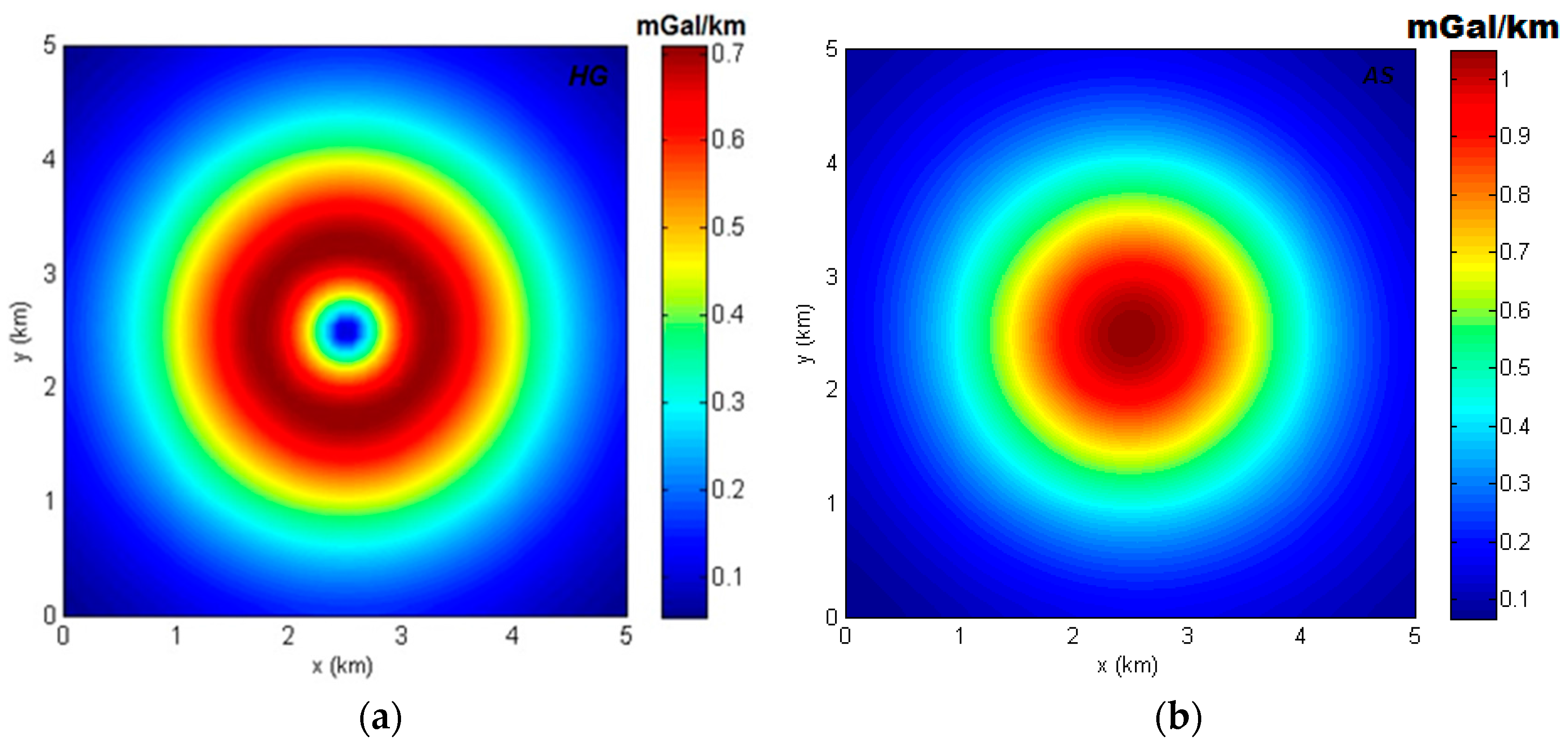
3.3.2. Horizontal Gradient and Analytic Signal Based on a Rectangular Prism

The analytic signal of potential field anomalies can be defined as complex fields of complex potential [24]. The concept of an analytic signal can be applied to magnetic and gravity data, as well as gradients in two or three dimensions. The analytic signal function is then applied to the x-, y-, and z-directions. The first vertical derivative amplitude of the analytic signal in the x- and y-directions can clarify the edge boundary of the anomalous object. The analytic signal A(x) of the potential field φ(x) is measured along the x-axis at a constant level caused by 2D strike along the y-axis, and its expression can be quantitatively written as [20]:
A ( x ) = ϕ ( x ) x + i ϕ ( x ) z ,
where ϕ ( x ) x and ϕ ( x ) z are the form of Hilbert transformation pairs. The amplitude of the analytic signal is:
| A ( x ) | = [ ϕ ( x ) x ] 2 + [ ϕ ( x ) z ] 2 .
The generalizing of the 2D analytic signal to 3D and it is shown that Hilbert’s transformation of a potential field satisfies the Cauchy–Riemann relationship. The definition of the potential field analytic signal φ(x, y) measured in the horizontal plane to 3D can be expressed as [25]:
A ( x , y ) = ϕ ( x , y ) x + ϕ ( x , y ) x + i ϕ ( x , y ) z .
The amplitude of A(x, y) is given by:
| A ( x , y ) | = [ ϕ ( x , y ) x ] 2 + [ ϕ ( x , y ) y ] 2 + [ ϕ ( x , y ) z ] 2 .
The quantity of analytic signal is a combination of horizontal vertical and horizontal derivatives of a potential field to detect the boundary of anomaly causing objects.
Based on the gravity anomaly response from the prism model, horizontal gradient and 3D analytic signal are performed. The aims of this analysis to obtain the edge and shape boundary of the rectangular prism object and reduce noise. The horizontal gradient is the sum of the x-gradient and y-gradient, while the analytic signal is a combination of horizontal gradient and z-vertical gradient. The horizontal gradient and analytic signal based on a rectangular prism model are shown in Figure 8.
The horizontal gradient and analytic signal are positive values due to the square roots of the x-, y-, and z-gradients. The horizontal gradient value ranges from 0.1 mGal/km to 0.7 mGal/km, while the analytic signal is in a range between 0.1 mGal/km to 1 mGal/km.

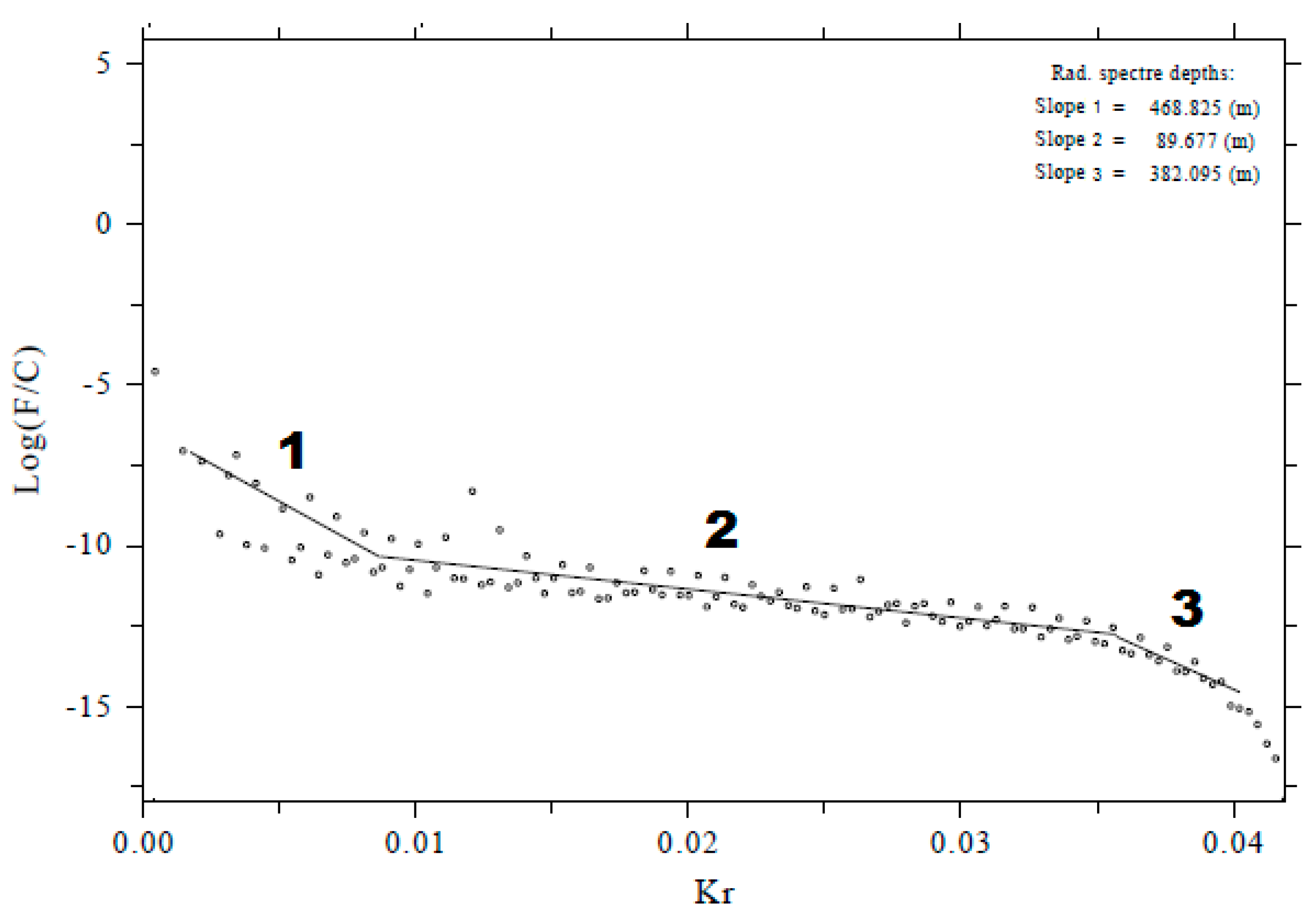
3.4. Depth Estimation and Anomaly Separation

Once the analytic signal was applied, the depth to these boundaries was estimated using 2D radial spectral analysis. The purpose of a spectral analysis is to characterize the preliminary depth and shape of gravity anomalies. Radial amplitude is calculated as the mean of 2D, and the Fourier amplitude spectrum is expressed as [23]:
A = | F | = | R e ( F ) 2 + I m ( F ) 2 | 1 / 2 ,
along the rings with the radius k r = [ k x 2 + k y 2 ] 1 / 2 centered on k x = k y = 0 . The amplitude spectrum analysis has generally been used to estimate the peak depth of the potential field source. This is done by making a linear line to the amplitude curve with a semi-logarithmic scale. In the frequency domain, the Fourier transform of a potential field data can be formulated as [23]:
F C e h k .
Log (F/C) = −hk. Thus, the depth (h) to the top of the surface is related to the tangent of the line that is fitted to the linear parts of the amplitude spectrum on a semi-logarithmic scale. The coefficient C depends on the selected data. For gravity data, C = −1/(kxkyk) and, for magnetic data, C = −1/(kxky) [23].
Bouguer anomaly is a combination of regional effects caused by deep structure and local effects by shallow structures [26]. This Bouguer anomaly needs to be separated according to the requirements of the study. An upward continuation method was used to separate regional anomalies and local anomalies. Upward continuation is an operation to move data with a constant high level above the earth’s surface (or measuring plane) and is used to estimate large-scale or regional trends (low frequencies or long wavelengths) of potential field data [26]. Some degree of upward continuation is the same as low-pass filtering because this process eliminates data with high frequency. Conversely, the downward continuation is an operation to shift data below the measurement plane. Downward continuation is used to increase the high-frequency data and to estimate the shallow depth of the target. The upward and downward continuation can be written as [23,27]:
F [ U u ] = F [ U ]   x   e Δ z . k   and   F [ U d ] = F [ U ]   x   e + Δ z . k ,
where F [ U ] , F [ U u ] , and F [ U d ] are the Fourier transforms of the potential field U . Upward continuation U u , downward continuation U d , Δ z > 0 is the elevation difference, and k = [ k x 2 + k y 2 ] 1 / 2 is the radial wave number.

4. Results

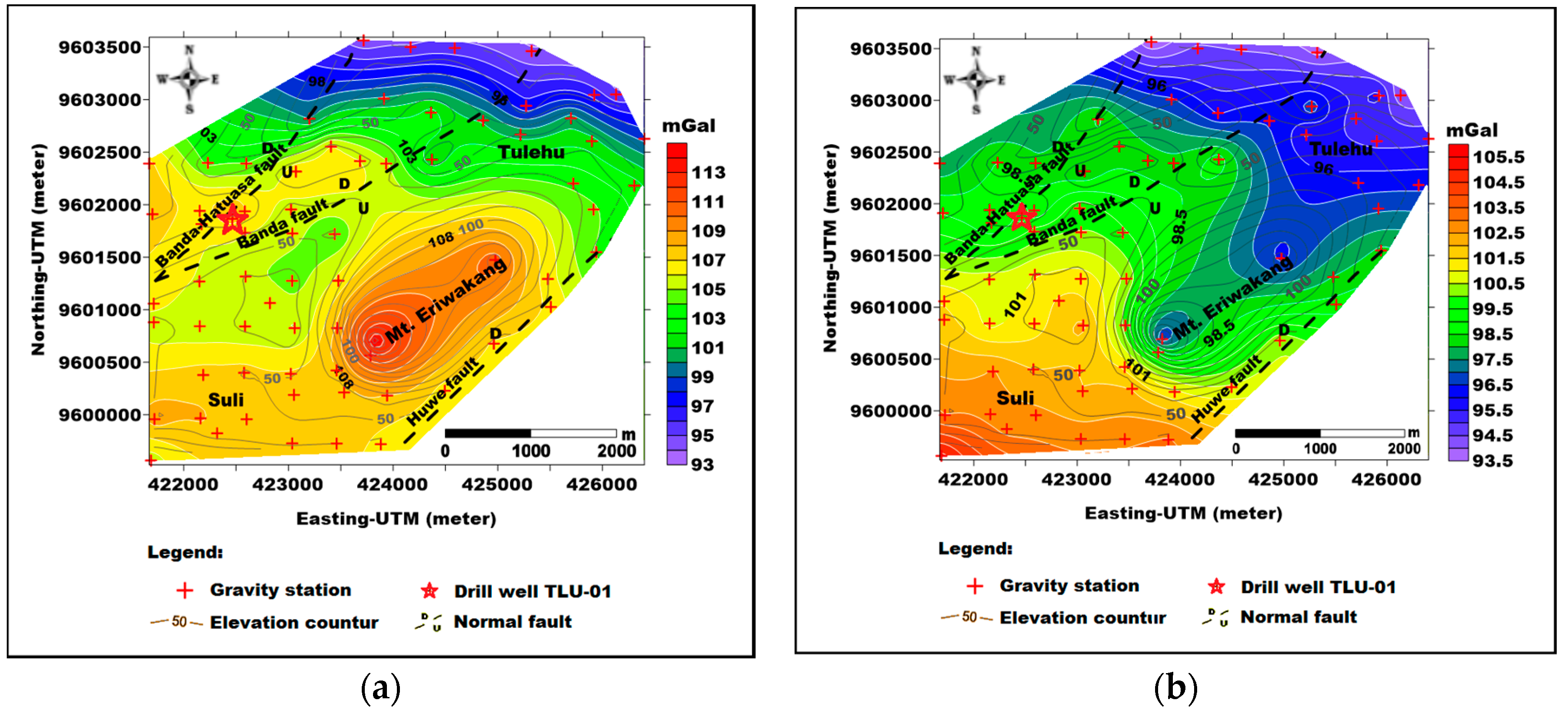
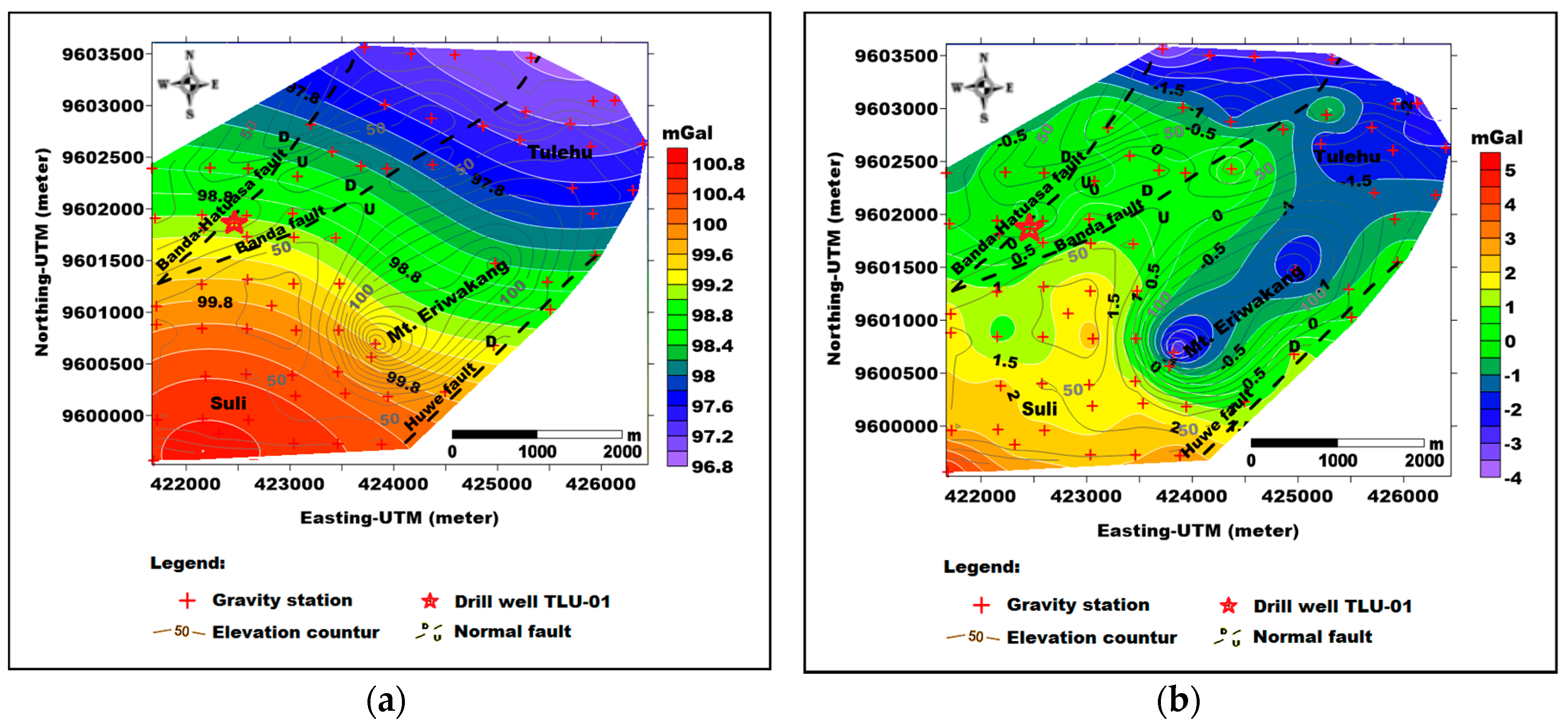
4.1. Gravity Variations

The result of gravity method data processing provided two important anomalies used for studying the geothermal system in Suli and Tulehu. We used a free air and a complete Bouguer anomalies data as references to describe anomaly variations of the gravity field (Figure 9).
The free air and complete Bouguer anomaly data were interpolated using the minimum curvature gridding approach. Figure 9a shows a free air anomaly map with a southwest to a northeast direction and variations ranging from 94 mGal to 114 mGal. In general, the form of free air anomalies correlates with the topography of the study area (Figure 2). The high free air anomaly is circular and founded on Eriwakang mountain, the values decrease in the Suli region and reach the lowest value in the Tulehu area.
Figure 9b shows the complete Bouguer anomaly map with the southwest to the northeast direction and for which gravity values range from 93 mGal to 105 mGal. High gravity anomalies with open contour patterns exist in the Suli region, and the circular pattern describes gravity decrease in Eriwakang mountain and reaches the lowest value in the Tulehu area. The gravity field variation in Eriwakang mountain has a moderate level of confidence because there is only a small amount of gravity data measurement. In general, the existence of geothermal manifestations and drill point of TLU-01 in Suli and Tulehu along fault lines, especially Banda-Hatuasa and Banda faults are associated with moderate gravity anomalies.

4.2. Deep Estimation and Anomaly Separation of Complete Bouguer Anomaly in Suli and Tulehu

The gravity anomaly spectrum of the Suli and Tulehu areas consists of three linear trends on the logarithmic scale (Figure 10).
The first linear trend is associated with a deep anomaly source in an estimated depth of 470 m (Figure 10). The second linear trend is associated with a shallow anomaly source with an approximate depth of 90 m, while the third linear trend is estimated as the background noise of the gravity data. According to the information of 2D radial power spectrum analysis, it is estimated that the upper layer of igneous rock intrusion in Suli and Tulehu geothermal areas is at a depth more than 500 m. Sedimentary rocks have a thickness of more than 90 m. This is supported by information obtained from TLU-01 drill hole analysis [3], and a 3D Magnetotellurik inversion model [5]. The result of 2D radial spectrum power analysis is then used as information in a forward modeling process in an initial model as a constraint and inversion modeling of earth gravity of Suli and Tulehu regions.
For the next interpretation, we have made a separation between the regional and residual anomalies, which are embedded within Bouguer anomaly. Regional gravity anomalies are generated by deep and large structures, whereas residual gravity anomalies are generated by shallow and small structures [8,28]. In this study, we are interested to reveal the shallow structure, so that the regional anomaly was removed.
We used the upward continuation method to separate the regional and residual anomalies. The upward continuation was carried out at a height of 1 km from the earth’s surface. This is based on the borehole TLU-01 depth information of 930 m and the depth estimation of anomaly based on 2D radial power spectrum analysis. The map of regional and residual anomalies from an upward continuation of 1000 m altitude from the Suli and Tulehu geothermal areas was shown in Figure 11.
Figure 11a shows the regional anomaly map with ranges 96 mGal to 101 mGal. The trend of regional anomaly decreases from southwest to northeast with open contour patterns. Figure 11b shows the residual anomaly with ranges −4 mGal to 5 mGal.
In general, residual anomaly patterns have similarities with a complete Bouguer anomaly pattern. This shows that the variations of gravity anomalies are largely influenced by local structures. The trend of residual anomaly decreases from southwest to northeast.

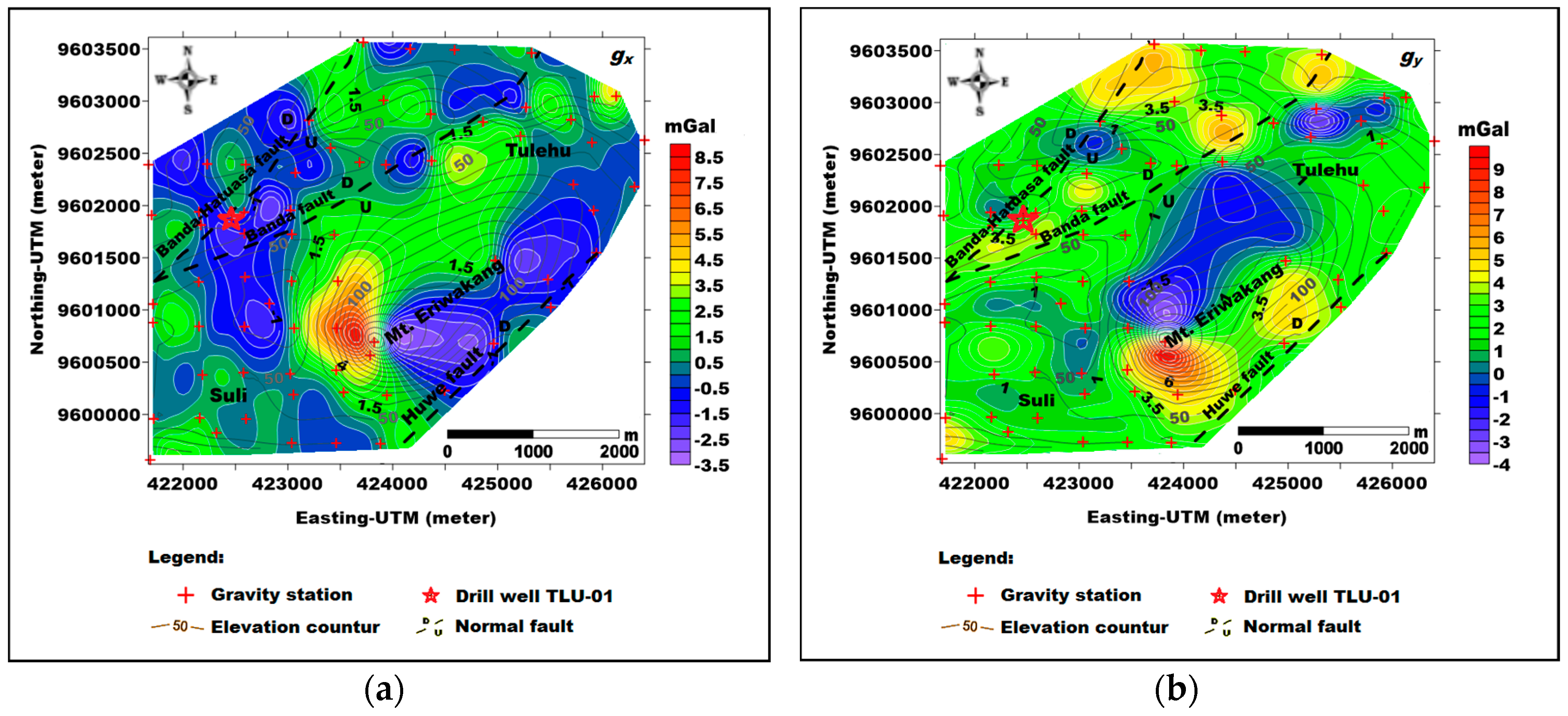
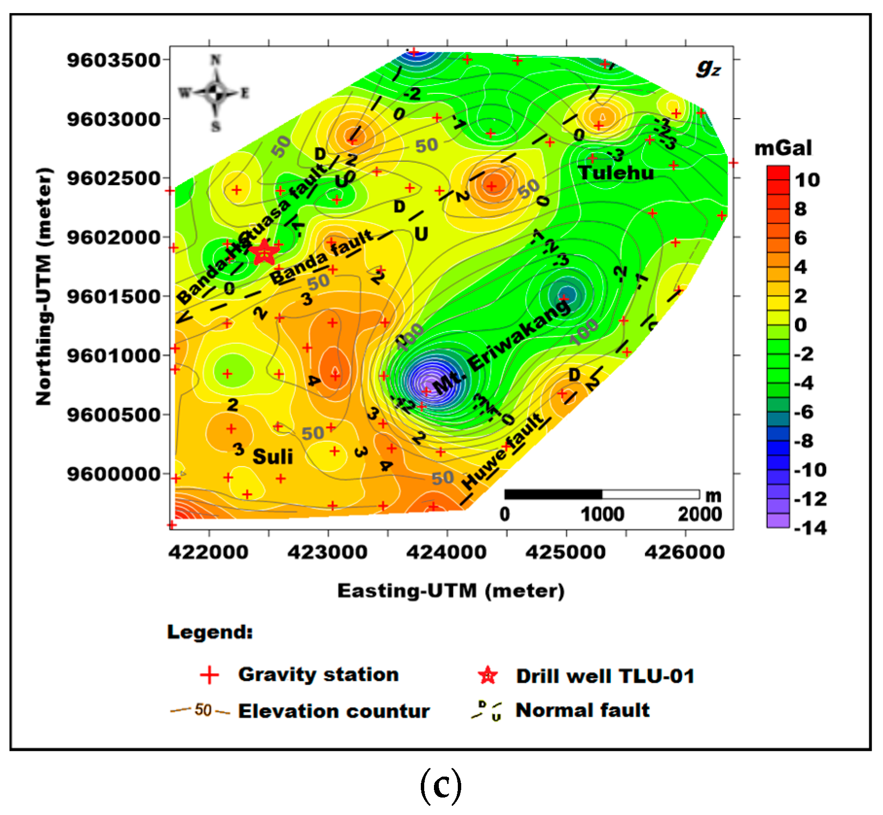
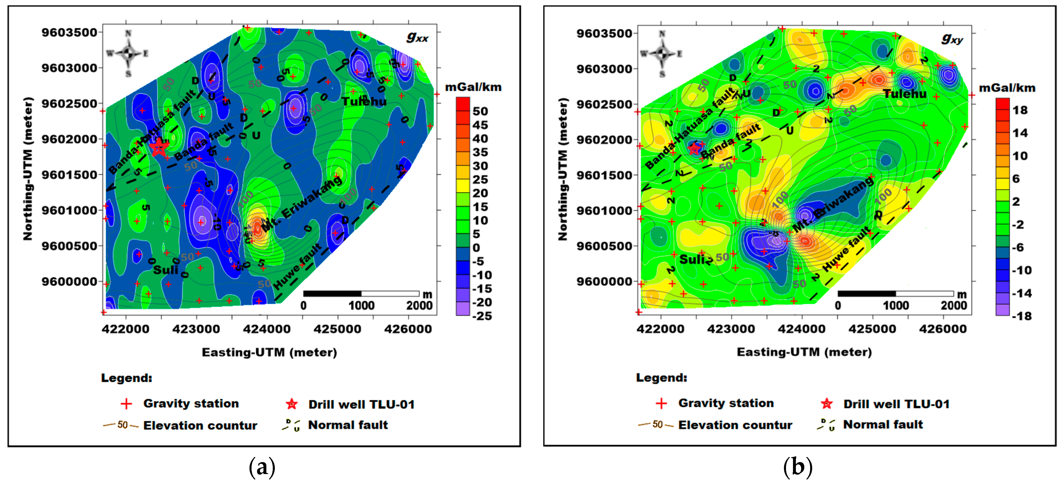
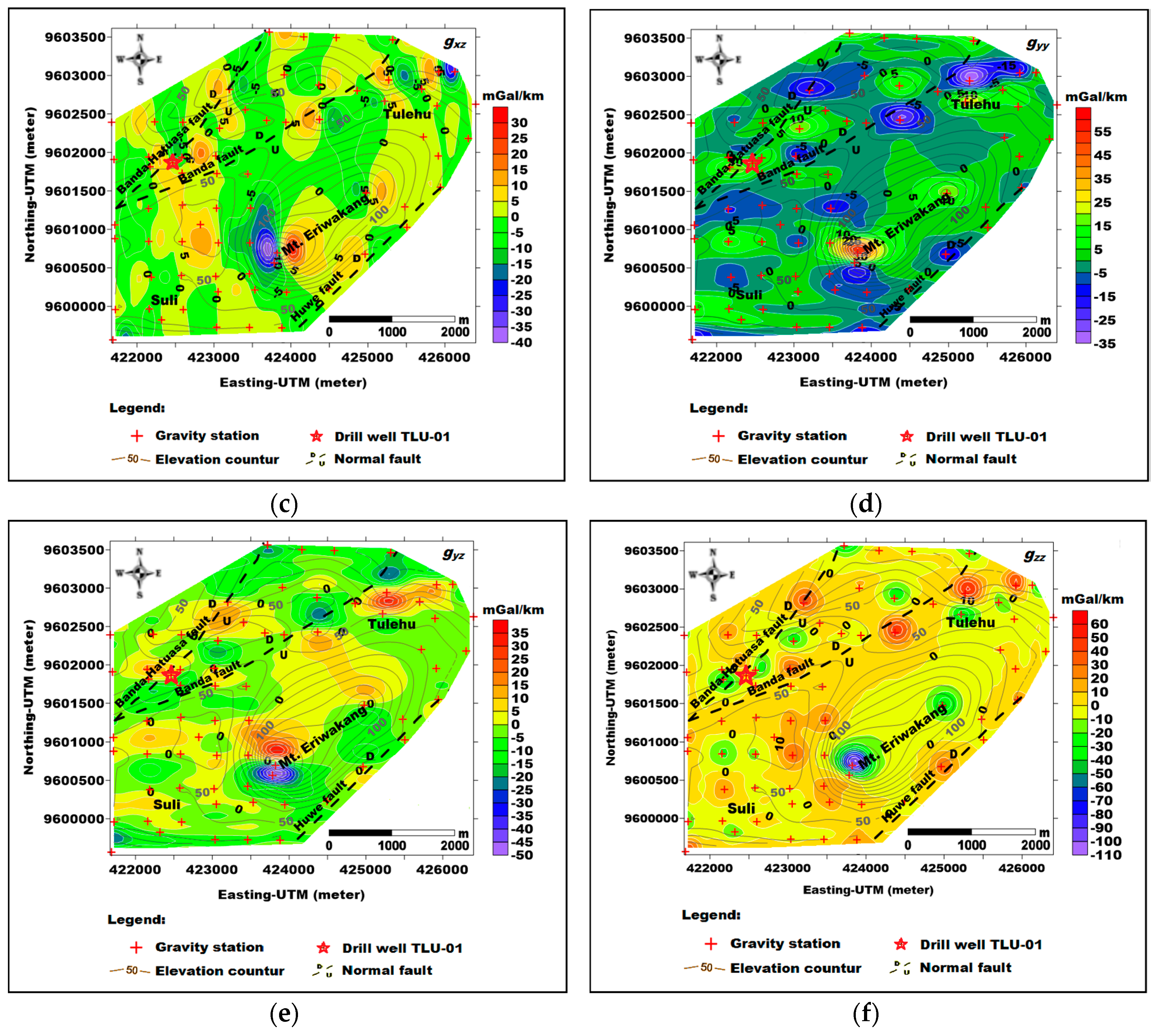
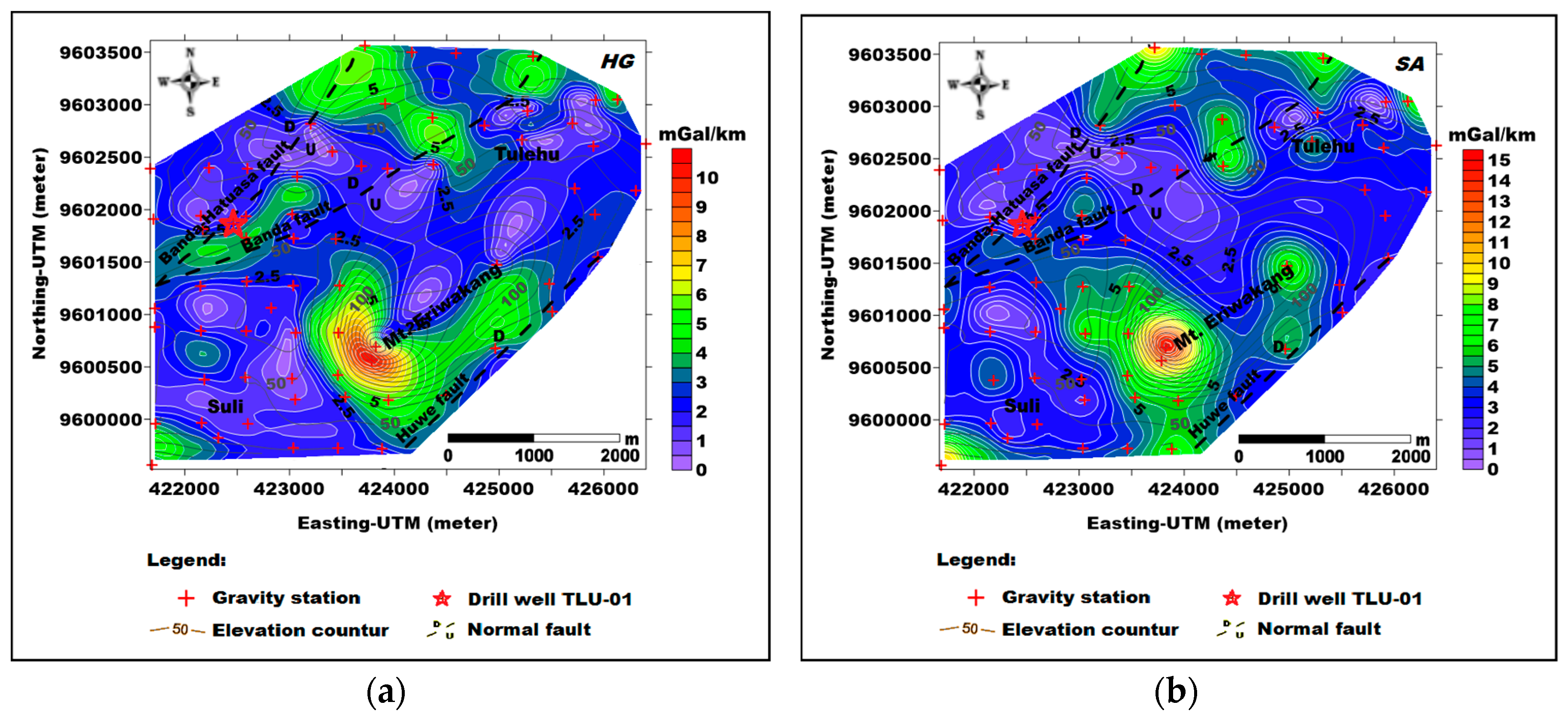
4.3. Gravity Gradient Tensor Analysis of Suli and Tulehu Geothermal Areas

The gravity gradient tensor and analytic signal were applied to complete Bouguer anomaly data over the study area. It was performed using fast Fourier transform by Fourpot software (version, Manufacturer, City, US State abbrev. if applicable, Country) [23]. The Fourier transform shows a sum of sine and cosine term with different spatial frequencies or wave number (kx, ky) that are defined by a sampling of data (dx and dy) along x- and y-directions [29]. We calculated the gravity potential field from the complete Bouguer anomaly over the study area.
Potential fields are defined as the (negative) gradient of corresponding scalar potential can be obtained from the vertical component of the field by dividing its Fourier transform by the radial wave number (k) [23]. Then, we calculated the first derivative of the gravity potential in the x-, y-, and z-directions. These derivatives are the horizontal (gx, gy) and vertical (gz) gravity components of the gravity field vector. The gravity anomalies components gx, gy, and gz over the study area have low values and present some more complex pattern (Figure 12).
The anomaly in the x-direction (gx) has a value of −3.387 mGal to 8497 mGal, the anomaly in the y-direction (gy) has a value of −3.677 mGal to 9501 mGal and the anomaly in the z-direction has a value of −13.946 mGal to 9.917 mGal. The gx component is dominated by lower (dark blue) to moderate gravity anomalies (green). The gy component is dominated by moderate (green) to high gravity anomalies (yellow); in some places, there is a lower (dark blue) anomaly like the northern part of Tulehu. The gz component is dominated by an increase anomaly in Suli and decrease anomaly in Tulehu. The pattern of gz component is similar to the complete Bouguer and residual anomalies. The geological structural boundaries in the gz component begin to be apparent.
The gravity gradient components of Suli and Tulehu areas are computed by taking the horizontal (x and y) and vertical (z) derivatives of the three gravity components. In the frequency domain, a gravity gradient tensor is computed by multiplying the Fourier transform of the anomaly field with wave numbers (kx, ky, kz). The six components of the gravity gradient tensor are shown in Figure 13.
The minimum and maximum values of gravity gradient tensor in the Suli and Tulehu regions were shown in Table 2.
Each component of the gravity gradient tensor has certain values and meanings related to the geological structure. When associated with a gravity gradient tensor based on synthetic modeling, it appears that gravity tensors present is a common pattern generated by the local gravity variation in the Suli and Tulehu regions.
In this research, horizontal gradient and analytic signal have been done to Bouguer gravity anomaly data in Suli and Tulehu geothermal areas. The purpose of horizontal gradient and analytic signal is to detect, estimate and clarify the shape and the border of the geological structure of the study area. Geothermal fields in many sedimentary basins are distributed along fault structures [26]. The results from the horizontal gradient and analytic signal of Suli and Tulehu geothermal regions are shown in Figure 14. The amplitude of horizontal gradient and analytical signal of the Suli and Tulehu regions are positive and range between 0.059 mGal/km to 10,551 mGal/km, whereas the analytic signal has an amplitude with a value between 0.306 mGal/km to 14,858 mGal/km.

5. Discussion

5.1. Relationship between Gravity Anomaly and Geological Features

Based on the local geological map of the Suli and Tulehu regions (Figure 2), the main geological structure over the study area is dominated by Ambon volcanic rocks covered by sedimentary rocks [1,3]. When compared to a complete Bouguer anomaly map of the study area (Figure 9b), it can be interpreted that a high gravity anomaly is mostly associated with lava andesite rocks in Suli that are estimated to have a high rock density. High gravity anomaly indicates strong intrusions of magmatic rocks below the Suli region. It is also supported by regional and residual anomalies of the Suli and Tulehu regions (Figure 11a), in which the highest gravity anomaly found in the Suli region. The TLU-01 drill hole analysis shows subsurface lithology composed of Tuff, breccia, and lava andesite [3].
On the other hand, the interpretation of MT methods indicates that the geological structure of the research area is formed by an old quaternary volcanic in Salahutu and young quaternary volcanic in Eriwakang, which mostly consist of andesite to dacite rocks, and probably a young heat source, indicated a shallow cooling magma chamber consisting of diorite to granodiorite [5]. The decrease of the gravity anomaly occurs in the Eriwakang mountain until Tulehu is associated with a coral limestone. The lower gravity anomalies are located in the north to the northeast part of Tulehu are associated with alluvium rocks that have a lower rock density.
The geological information of the study area indicates that the geothermal manifestations of hot springs are in the fault zone as controllers [1,3,5]. The fault structures are dominated by normal faults such as Banda fault, Banda-Hatuasa fault, and Huwe fault with an orientation of southwest to northeast. These faults arise from the subduction of the Australian plate under the Eurasian plate on the south of Ambon Island, which is associated with the Seram trough [30]. The normal fault in the research area generally results from the opening zone or fracture zone that becomes the path of geothermal fluid circulation. On the other hand, the faults and fractures resulting in a reduction of rock density value associated with a decrease in gravity anomaly.
In the complete Bouguer anomaly, the geothermal manifestation of the fault zone (Banda and Banda-Hatuasa faults) is in a moderate gravity anomaly from northeast to southwest. The shape and boundaries of the geological feature and fault zone are not clearly illustrated on the complete Bouguer anomaly map of this area, so some approach is needed to overcome it such anomaly separation and gradient analysis.
Several studies suggest that in geothermal exploration using gravity methods (not in all cases), negative gravity anomaly zones may be directly related to a fault and fracture zone or geothermal reservoirs [8,28]. The complete Bouguer anomaly also has not been able to explain the existence of a low anomaly or negative zone associated with geothermal manifestations of the faults and fractures structures in Suli and Tulehu.
To illustrate that the existence of fault structures have carried out the separation of regional and residual anomalies through an upward continuation, the residual anomaly interpretation (Figure 11b) shows that the manifestations and geothermal point of TLU-01 along the fault lines, especially in the Banda, and Banda-Hatuasa faults are low anomalies (negative zone). The residual anomaly pattern has a similar to the complete Bouguer anomaly so that variations of gravity anomaly are largely influenced by more complex shallow structures. In general, the geological features of the study area are clearer on the residual anomaly map, but, in some places, the alignment pattern of the fault and other structures have not been seen clearly.

5.2. Significance of Using Gravity Gradient in Understanding the Suli and Tulehu Geothermal Areas

We have developed this study to learn about the geothermal system in Suli and Tulehu areas based on gravity gradient tensor and an analytic signal. The goal is to obtain the geological structure in more detail of all directions’ gradient components. Conventional gravity data measurements show the magnitude of the earth’s gravitational field but are less sensitive to determine the limitations of anomalies’ objects, and they do not have directional information [9]. On the other hand, we used the result of gravity gradient tensor and an analytic signal as the input and constraint to quantitative interpretation based on subsurface modeling of the geothermal system over the study area in the next research.
For the initial approach, we used the forward modeling of the single rectangular prism (Figure 4) to get an understanding of the anomaly response of the gravity field and its gradients (Figure 5). Previous research on gravity gradient tensor and analytic signal has been done through a rectangular prism model with different density contrast [9,11,12]. We use a rectangular prism because, for a complex geometries model, it can be built easily through the approximation of a set of similar prisms, and has an analytical solution to calculate the gravitational response. By using a prism, the density distribution of 3D objects can be approximated with the desired accuracy. The density may be given to each prism freely by any neighbouring prism density [9,31,32].
The rectangular prism that was made has a positive density contrast. This is done to illustrate the existence of magmatic rock intrusion as the main source of heat energy in the research area. The intrusion of magmatic rock can produce the positive gravity anomaly (Figure 7). Figure 5 shows a circular synthetic gravity anomaly response with the highest value being at the centre of the circle. In this form, the anomaly response has not been able to explain the shape, edge, and the boundary of the rectangular prism because the overall anomaly is still dominated by the influence of regional trends.
The gx component (Figure 6a) shows the maximum and minimum pattern from the west to east. The western–eastern boundary of the rectangular prism has not been clearly visible in this anomaly. The gy component (Figure 6b) shows the maximum and minimum pattern from north to south. The northern–southern boundary of the rectangular prism has not been seen clearly. The gz component (Figure 6c) shows the overall pattern of the prism but has not been explicit showing the edge, boundaries, and the corners of the prism. This is because most of the anomalies produced are still influenced by the regional trend. Thus, in order to get the detailed model of rectangular prisms, we produced in the gradient tensor components and an analytic signal of the anomaly response.
The gravity gradient and analytic signal essentially are a high-frequency filter, which further enhances residual anomalies and eliminate or remove regional anomalies. For our testing model, the rectangular prism produces a small gravitational field anomaly response. This response can cause the element of the gravity field in x-, y-, and z-directions to also be small. All gravity gradient components provide clearer information about the shape, edges, and boundaries of the rectangular prism (Figure 7). This argument is supported also by the results of the horizontal gradient and analytic signal of the rectangular prism (Figure 8). A geothermal system investigation of Suli and Tulehu based on the forward modeling of the single rectangular prism has its drawbacks because the results obtained are too simple and not complex. This result is a preliminary study that will be developed using a combination of multiple prisms as the initial model for forward modeling of the subsurface structures’ investigation of the geothermal system over the study area.
The application of gravity gradient tensor and analytic signal to the complete Bouguer anomaly data of the Suli and Tulehu regions gets information about the geological structural boundaries prevailing in the area. Each gradient component has a more complex pattern that associates with a shallow structure and removes deeper regional influences. The value of a gravity gradient tensor obtained is relatively small with a negative to a positive anomaly in mGal/km. Each gradient component can explain the existence of Banda and Banda-Hatuasa fault structures and the intrusion zone associated with geothermal manifestations in the Suli and Tulehu regions. These boundaries of these geological features are clear on the gzz gradient component associated with the zero value (Figure 13f).

6. Conclusions

The result of gravity data processing and interpretation shows that the complete Bouguer anomaly decreases from the southwest in Suli to the northeast in Tulehu. A high gravity anomaly in Suli indicates a strong magmatic rocks intrusion. The gravity anomalies decrease occurs on the Eriwakang mountain and most of Tulehu is associated with coral limestone. The lower gravity anomalies in the north to northeast part of Tulehu are indicated with alluvium. The drill well TLU-01 and a geothermal manifestation along the Banda and Banda-Hatuasa faults are associated with lowest gravity anomaly. Our result shows that the gravity gradient tensor simulation and analytic signal over the study area are small from negative to positive. All of the gravity gradient components give more detailed information about the geological features in Suli and Tulehu areas, especially in the gzz component. On the other side, these results will be used as inputs and geophysical constraints to create the subsurface geological model based on gravity gradient inversion modeling.

Acknowledgments

The authors would like to thank the Ministry of Research, Technology and Higher Education of the Republic of Indonesia, which has provided an opportunity for doctoral education by awarding a scholarship in 2014 and a doctoral research grant in 2017 at Universitas Gadjah Mada. The authors also thank the government of Maluku province and PT. PLN Maluku and North Maluku regions have given permission to conduct our research in Suli and Tulehu. We also thank M. Ozgu Arisoy and Unal Dikmen, who have developed the potential field data processing software ‘POTENSOFT’ that can be used for free to facilitate the completion of this paper. The authors also thank Markku Pirttijarvi, who has developed the FOURPOT software for 2D fast Fourier transform analysis.

Author Contributions

R.L. and A.S. conceived the idea for this study and designed the gravity data acquisition; R.L. and a technician performed the experiments; R.L. wrote the paper with contributions from all co-authors; S.S., A.S., and S.P. reviewed the paper.

Conflicts of Interest

The authors declare no conflict of interest.

References

  1. Sari, A.W.I.; Vandani, C.P.K.; Mulyaningsih, E.; Warmada, W.I.; Utami, P.; Yunis, Y. Studi alterasi hidrotermal bawah permukaan lapangan panas bumi “BETA”, Ambon dengan metode X-ray Diffraction. In Proceedings of the Seminar Nasional Kebumian KE-7, Yogyakarta, Indonesia, 30–31 October 2014. [Google Scholar]
  2. Munandar, A.; Risdianto, D.; Nursahan, I. Pengembangan Energi Panas Bumi Daerah-Daerah Pulau Terisolir. Badan Geologi Indonesia. 2017. Available online: http://www.bgl.esdm.go.id/index.php?option=com_content&task=view&id=654&Itemid=1&date=2021-11-01 (accessed on 15 November 2017).
  3. Vandani, K.P.C.; Sari, A.W.I.; Mulyaningsih, E.; Utami, P.; Yunis, Y. Studi alterasi hidrotermal bawah permukaan di lapangan panas bumi “BETA”, Ambon dengan metode Petrografi. In Proceedings of the Seminar Nasional Kebumian KE-7, Yogyakarta, Indonesia, 30–31 October 2014. [Google Scholar]
  4. Curewitz, D.; Karson, A.J. Structural settings of hydrothermal outflow: Fracture permeability maintained by fault propagation and interaction. J. Volcanol. Geotherm. Res. 1997, 79, 149–168. [Google Scholar] [CrossRef]
  5. Nasution, A.; Aviff, M.; Nugroho, S.; Yunis, Y.; Honda, M. The Preliminary Conceptual Model of Tolehu Geothermal Resource, Based on Geology, Water Geochemistry, MT, and Drilling; Proceedings World Geothermal Congress: Melbourne, Australia, 2015. [Google Scholar]
  6. Gottsman, J.; Camacho, G.A.; Marti, J.; Wooller, L.; Fernandez, J.; Garcia, A.; Rymer, H. Shallow structure beneath the Central Volcanic Complex of Tenerife from new gravity data: Implications for its evolution and recent reactivation. Phys. Earth Planet. Inter. 2008, 168, 212–230. [Google Scholar]
  7. Represas, P.; Santos, M.A.F.; Ribeiro, J.; Ribeiro, A.J.; Almeida, P.E.; Goncalves, R.; Moreira, M.; Victor-Mendes, A.L. Interpretation of gravity data to delineate structural features connected to low-temperature geothermal resources at Northeastern Portugal. J. Appl. Geophys. 2013, 92, 30–38. [Google Scholar]
  8. Moghaddam, M.M.; Mirzaei, S.; Nouraliee, J.; Porkhial, S. Integrated magnetic and gravity surveys for geothermal exploration in Central Iran. Arab. J. Geosci. 2016, 9, 1–12. [Google Scholar]
  9. Dubey, P.C.; Tiwari, M.V. Computation of the gravity field and its gradient: Some applications. Comput. Geosci. 2016, 88, 83–96. [Google Scholar] [CrossRef]
  10. Kohrn, B.S.; Bonet, C.; Difrancesco, D.; Gibson, H. Geothermal Exploration Using Gravity Gradiometry—A Salton Sea Example. Geotherm. Resour. Counc. Trans. 2011, 35, 1699–1702. [Google Scholar]
  11. Grandis, H.; Dahrin, D. Full Tensor Gradient of Simulated Gravity Data for Prospect Scale Delineation. J. Math. Fundam. Sci. 2014, 46, 107–124. [Google Scholar]
  12. Mickus, L.K.; Hinojosa, J.H. The complete gravity gradient tensor derived from the vertical component of gravity: A Fourier transform technique. J. Appl. Geophys. 2001, 46, 159–174. [Google Scholar] [CrossRef]
  13. Holis, Z.; Ponkarn, S.A.; Gunawan, A.; Damayanti, S.; Gunawan, K.B. Structural Evolution of Banda Arc, Eastern Indonesia: As a Future Indonesian Main Oil and Gas Development. In Proceedings of the Poster Presentation at AAPG International Convention and Exhibition, Singapore, 16–19 September 2012. [Google Scholar]
  14. Pairault, A.A.; Hall, R.; Elders, F.C. Structural styles and tetonic evolution of the Seram Trough, Indonesia. Mar. Pet. Geol. 2003, 20, 1141–1160. [Google Scholar] [CrossRef]
  15. Charlton, R.T. The Pliocene-Recent Anticlockwise Rotation of the Bird’s Head, the Opening of the Aru Trough—Cendrawasih Bay Spenochasm, and the Closure of the Banda Double Arc. In Proceedings of the IPA Thirty-Fourth Annual Convention an Exhibition, Jakarta, Indonesia, 18–20 May 2010. [Google Scholar]
  16. Honthaas, C.; Maury, C.R.; Priadi, B.; Bellon, H.; Cotton, J. The Plio-Quaternary Ambon arc, Eastern Indonesia. Tectonophysics 1999, 301, 261–281. [Google Scholar] [CrossRef]
  17. Van Bemmelen, R.W. The Geology of Indonesia; Government Printing Office: The Hague, The Netherlands, 1949; Volume 1, p. 732.
  18. Marini, L.; Susangkyono, E.A. Fluid geochemistry of Ambon Island (Indonesia). Geothermics 1999, 28, 189–204. [Google Scholar] [CrossRef]
  19. Jacoby, W.; Smilde, L.P. The gravity tensor (Eotvos Tensor) Gravity Interpretation. In Fundamentals and Application of Application of Gravity Inversion and Geological Interpretation, 1st ed.; Springer: Berlin/Heidelberg, Germany, 2009; Volume 1, pp. 45–46. ISBN 978-3-540-85328-2. [Google Scholar]
  20. Beiki, M. Analytic signal of gravity gradient tensor and their application to estimate source location. Geophysics 2010, 75, 159–174. [Google Scholar] [CrossRef]
  21. Saibi, H.; Nishijima, J.; Ehara, S.; Aboud, E. Intergrated gradient interpretation techniques for 2D and 3D gravity data interpretation. Earth Planets Space 2006, 58, 815–821. [Google Scholar] [CrossRef]
  22. Arisoy, O.M.; Dikmen, U. Potensoft; MATLAB-based software for potenstial data processing, modeling and mapping. Comput. Geosci. 2011, 37, 935–942. [Google Scholar] [CrossRef]
  23. Pirttijarvi, M. FOURPOT: Potential Field Data Processing and Analysis of Using 2D Fourier Transform. Manual Software. 2014. Available online: https://wiki.oulu.fi/display/~mpi/ (accessed on 15 November 2017).
  24. Ansari, H.A.; Alamdar, K. A new edge detection method based on the analytic signal of tilt angle (ASTA) for magnetic and gravity anomalies. Iran. J. Sci. Technol. 2011, 35, 81–88. [Google Scholar]
  25. Roest, R.W.; Verhoel, J.; Pikington, M. Magnetic interpretation using the 3D analytic signal. Geophysics 1992, 57, 116–125. [Google Scholar] [CrossRef]
  26. Nishijima, J.; Naritomi, K. Interpretation of gravity data to delineate underground structure in the Beppu geothermal field, central Kyushu, Japan. J. Hydrol. Reg. Stud. 2017, 11, 84–95. [Google Scholar] [CrossRef]
  27. Blakely, J.R. Transformation. In Potential Theory in Gravity and Magnetic Applications, 1st ed.; Cambridge University Press: Cambride, UK, 1996; Volume 1, pp. 316–319. [Google Scholar]
  28. Nouraliee, J.; Porkhial, S.; Moghaddam, M.M.; Mirzaei, S.; Ebrahimi, D.; Rahmani, R.M. Investigation of density contrasts and geologic structures of hot springs in the Markazi Province of Iran using the gravity method. Russ. Geol. Geophys. 2015, 56, 1791–1800. [Google Scholar] [CrossRef]
  29. Khalil, A.M.; Santos, M.F.; Farzamian, M.; El-Kenawy, A. 2D Fourier transform analysis of the gravitational field of Northern Sinai Peninsula. J. Appl. Geophys. 2015, 115, 1–10. [Google Scholar] [CrossRef]
  30. Spicak, A.; Matejkova, R.; Vanek, J. Seismic response to recent tectonic processes in the Banda Arc region. J. Asian Earth Sci. 2013, 64, 1–133. [Google Scholar] [CrossRef]
  31. Abdeslem, G.J. The gravitational attraction of a right rectangular prism with density varying with depth following a cubic polynomial. Geophysics 2005, 70, J39–J42. [Google Scholar] [CrossRef]
  32. Nagy, D.; Papp, G.G.; Benedek, J. The gravitational potential and its derivatives for the prism. J. Geodesy 2000, 74, 552–560. [Google Scholar] [CrossRef]
Figure 1. The geological map of Suli and Tulehu geothermal areas, Ambon Island, Eastern Indonesia (This map was modified from [1,3]).
Geosciences 08 00004 g001
Figure 2. The research location of Suli and Tulehu geothermal areas in Ambon Island, Maluku province.
Geosciences 08 00004 g002
Figure 3. Gravity field and GPS measurements in Suli and Tulehu, (a) gravity base station at Suli village; (b) GPS base station at Suli village; (c) the gravity field and GPS measurement in one of the stations.
Geosciences 08 00004 g003
Figure 4. The perspective view of prisms model with size 1 km3 at 1 km depth with 0.43 g/cm3 of the density contrast (a) a plan view; (b) 3D view.
Geosciences 08 00004 g004
Figure 5. The theoretical response of potential anomaly with size 1 km3 at 1 km depth with 0.43 g/cm3 of the density contrast (a) a plan view; (b) 3D view.
Geosciences 08 00004 g005
Figure 6. The gravity field anomaly components based on rectangular prism in Cartesian system coordinates (a) gx; (b) gy; (c) gz.
Geosciences 08 00004 g006
Figure 7. The gravity gradient tensor obtained from forward modeling calculation of the rectangular prism model, (a) gxx; (b) gxy; (c) gxz; (d) gyy; (e) gyz; (f) gzz.
Geosciences 08 00004 g007
Figure 8. (a) the horizontal gradient of a rectangular prism; (b) analytic signal of a rectangular prism.
Geosciences 08 00004 g008
Figure 9. The gravity anomalies map of Suli and Tulehu geothermal areas (a) a free air anomaly; (b) a complete Bouguer anomaly.
Geosciences 08 00004 g009
Figure 10. The 2D radial spectrum of complete Bouguer anomaly in Suli and Tulehu geothermal areas. Point 1 showed the slope of deep-seated sources, point 2 showed the shallow-seated sources, and point 3 showed the noise of the data.
Geosciences 08 00004 g010
Figure 11. The anomalies separation using the upward continuation of 1 km on Suli and Tulehu geothermal areas (a) a regional anomaly; (b) a residual anomaly.
Geosciences 08 00004 g011
Figure 12. The gravity field components of Suli and Tulehu areas in Cartesian coordinate system (a) gx; (b) gy; (c) gz.
Geosciences 08 00004 g012aGeosciences 08 00004 g012b
Figure 13. The gravity gradient tensor in Suli and Tulehu geothermal areas, (a) gxx; (b) gxy; (c) gxz; (d) gyy; (e) gyz; (f) gzz.
Geosciences 08 00004 g013aGeosciences 08 00004 g013b
Figure 14. (a) the horizontal gradient; (b) 3D analytic signal of Suli and Tulehu geothermal regions.
Geosciences 08 00004 g014
Table 1. The value of the gravity gradient tensor based on rectangular prism model.
Gradient ComponentsMinimum (mGal/km)Maximum (mGal/km)
gxx−1.4890.465
gxy−0.4950.495
gxz−1.0811.081
gyy−1.4890.465
gyz−1.0811.081
gzz−0.2501.689
Table 2. The value of the gravity gradient tensor in Suli and Tulehu geothermal areas.
Gradient CmponentsMinimum (mGal/km)Maximum (mGal/km)
gxx−23.07346.522
gxy−17.96117.099
gxz−39.93429.058
gyy−33.69356.786
gyz−49.769A35.051
gzz−103.07251.843

