Applying the Coastal and Marine Ecological Classification Standard (CMECS) to Nearshore Habitats in the Northeastern Gulf of Mexico

Coastal and Marine Laboratory, Florida State University, St. Teresa, FL 32358, USA
†
Current Address: Marine Sciences Programme, University of Trinidad and Tobago, Chaguaramas, Trinidad and Tobago, West Indies.
Geosciences 2018, 8(1), 22; https://doi.org/10.3390/geosciences8010022
Submission received: 13 November 2017
/
Revised: 10 January 2018
/
Accepted: 12 January 2018
/
Published: 16 January 2018
Abstract
:Many countries have classification standards for their environmental resources including criteria for classifying coastal and marine ecosystems. Until 2012, the United States just had a nationwide protocol for classifying terrestrial and aquatic habitats with no national standard for marine and most coastal habitats. In 2012 the Coastal and Marine Ecological Classification Standard (CMECS) was implemented to address this need. In the past, coastal and marine classifications were developed at the regional or local level. Since its inception, the CMECS has not been applied in many geographic areas. My study was one of the first to apply the CMECS to the benthic habitats in the nearshore Northeastern Gulf of Mexico. Sidescan sonar mapping and dive surveys were completed at 33 sites at depths 10–23 m. Hardbottom and sand habitats characterized the study area, and the underwater surveys revealed hard corals, sponges, and macroalgae as the dominant taxa on the hardbottom. The CMECS was applied to the overall study area rather than each individual site or groups of similar sites because habitat and environmental characteristics, primarily outside the context of the CMECS, appeared to influence the distribution of taxa across sites more than the CMECS geoform, substrate, and water column components. The CMECS worked well for classifying the entire study area, but was not adequate for classifying the complex fine-scale habitats and temporal variations observed; modifications to the CMECS could help resolve these issues.
1. Introduction
Climate change, overfishing, habitat destruction, and pollution, including oil spills, are affecting marine resources. The potentially adverse effects of these human activities on marine organisms and their habitats are critical issues that need to be addressed. It is important that we conserve and manage our marine resources appropriately. However, the data available to make effective management decisions at relevant scales are often inadequate or do not even exist. In order to understand how humans are impacting marine ecosystems and what management strategies should be put in place, it is important to know the composition of the ecosystem and where habitats exist. Thus, the acquisition of detailed habitat classification maps should be the foundation for any environmental or ecological research program or management scheme. To create useful maps, the significant geologic, biologic, and environmental components of habitats in the region of interest should be identified and measured. Such classifications include information at various scales, and help identify sensitive areas and environmental issues. Detailed multi-scale maps provide powerful tools to managers, stakeholders, researchers, and the general public. The net result is a better understanding of the problems and their impacts while also generating wider support for effective conservation measures.
Habitat classification systems have been used extensively in terrestrial environments and remote sensing has made these classifications easier over broad areas and at multiple scales. With increased sensor resolution, more detailed classifications are now possible over wide spatial scales. The United States Geological Survey (USGS) “Land Use and Land Cover Classification System” was developed in the 1970s and is widely accepted and used for many terrestrial and aquatic applications [1,2]. Classification maps are primarily generated from high-resolution aerial photographs. Comparable high-resolution remote sensing technology in the form of acoustic imagery has been available for the marine environment for a few decades now, but prior to 2012 in the United States (U.S.), there was no standard marine classification system in place like the one developed by USGS for terrestrial applications. The Coastal and Marine Ecological Classification Standard (CMECS) was adopted by the Federal Geographic Data Committee (FGDC) in 2012 to fill the gap in the U.S. classification system [3]. Other similar national classification systems exist throughout the world. For example, the European Nature Information System (EUNIS) assigns hierarchical classifications to the aquatic, terrestrial, and marine habitats within and adjacent to Europe [4]. The United Kingdom, Australia, and New Zealand also have national classification systems [5].
Prior to the implementation of the CMECS system in the U.S., a plethora of classification systems were developed and used to classify marine habitats [6,7,8,9,10,11]. Most of these marine classification systems were only applied at local or regional scales, although some proposed that their systems could be effective in other areas, or even nationally [6,7,8,9,10,11]. However, as Auster et al. [1] reported, application of many of the available classification standards in 2009 was not possible without modifications for their study area, Long Island Sound. It appears that many marine classification systems were created because they were only useful in the area where they were applied. Due to the challenge of developing a classification system that can effectively classify all marine habitats in U.S. waters, efforts are ongoing to improve CMECS, so that users across the country can implement it and make meaningful spatial and temporal comparisons [3].
Classification systems provide an organized and systematic means for assigning habitats at a wide range of scales. The scales can range from broad geological or physical characteristics to detailed benthic community and substrate descriptions. For this reason, habitats are typically classified using hierarchical systems as demonstrated in the following examples. In Mumby and Harborne [8], habitats were arranged hierarchically based on their geomorphological structure and then benthic cover. Briones [10], on the other hand, started by broadly classifying Gulf of Mexico habitats into seven physiographic provinces (1) coastal lagoons, bays, and estuaries; (2) beaches and rocky coasts; (3) inner shelf; (4) outer shelf; (5) continental slope; (6) escarpments; and (7) abyssal plain, and then subdivided each of these provinces into more descriptive categories. Greene et al. [7] divided habitats into megahabitats, mesohabitats, and macrohabitats. Megahabitats encompassed areas at the scale of kilometers and larger [7]. Mesohabitats were smaller than megahabitats, tens of meters to a kilometer, and typically provided more geomorphological characteristics and associated fish communities [7]. Mesohabitats were then subdivided into macrohabitats at the scale of one to ten meters and included details on the substrate structure and associated communities [7].
The CMECS is also hierarchical and starts by assigning areas to biogeographic and aquatic settings [3]. The biogeographic setting includes a realm unit that is divided into provinces and then the provinces are classified into ecoregions based on climate, location, and evolutionary history [3]. For the aquatic setting, first a system is assigned then a subsystem and, finally, a tidal zone. The CMECS is then further subdivided into four main components: the water column, geoform, substrate, and biotic components [3]. The reader may navigate these settings and components in more detail on the CMECS website (http://www.cmecscatalog.org/).
The objectives for this study were to apply the CMECS to the benthic habitats in the nearshore Northeastern Gulf of Mexico and to see how well the CMECS performed in this region using seasonal dive surveys and sidescan sonar imagery. Biogeographic and aquatic settings were assigned and the classification included each of the four components discussed above to the lowest level possible with the data available.
2. Materials and Methods
2.1. Study Area
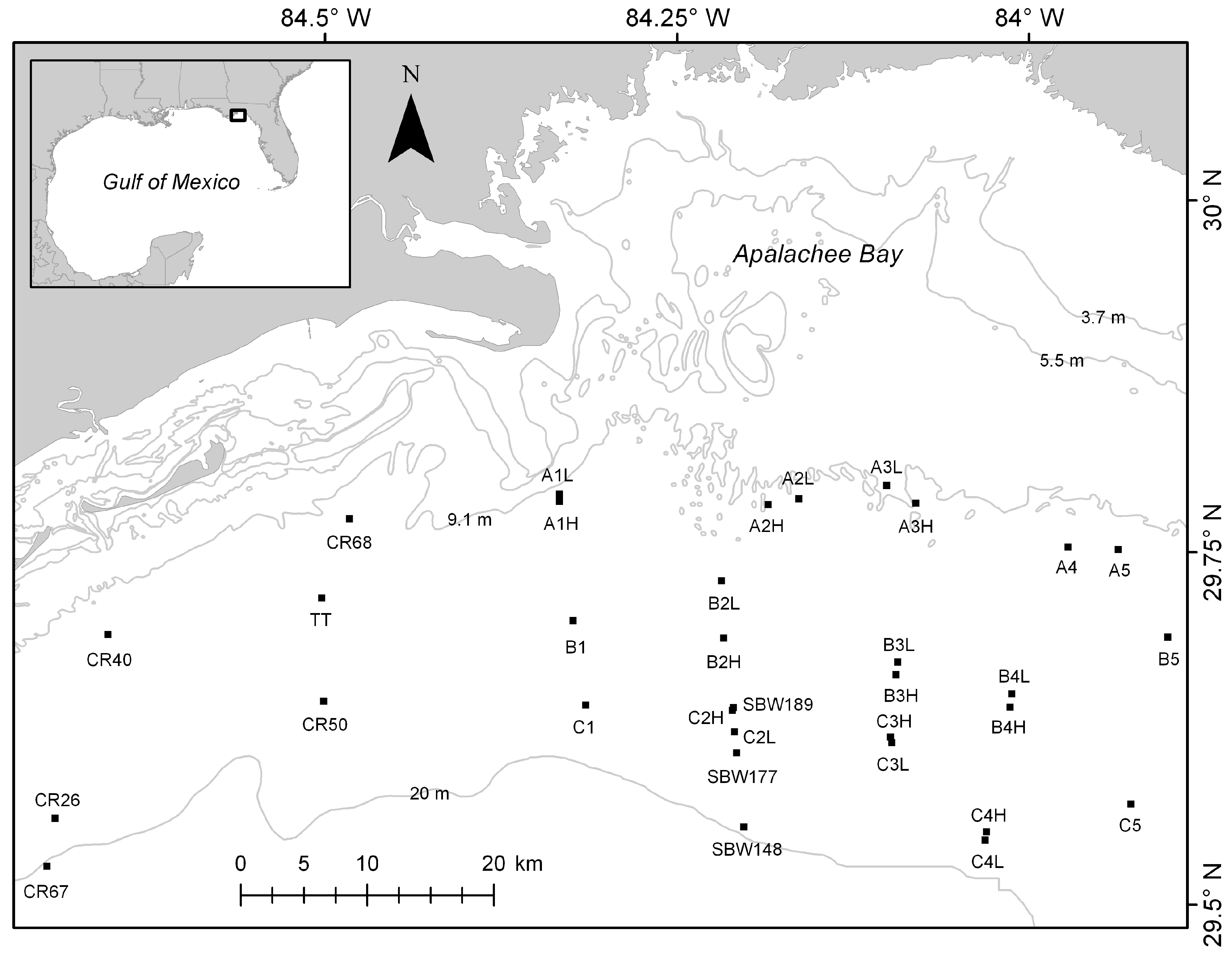
The location of this study was the nearshore marine areas of the Northeastern Gulf of Mexico off the coast of Northwest Florida (Figure 1). The seafloor in this region is primarily drowned karst with sand, limestone, and detrital sediments [12]. The continental shelf is wide (up to 188 km across) and gently sloped [12]. Currents, fronts, and waves affect the region at a variety of temporal scales from hourly changes from semi-diurnal tidal currents to the occasional storm surge that accompanies tropical systems that hit the area on an annual, or longer time scale.
Nearshore benthic habitats generally consist of sand and limestone hardbottom. Hardbottom refers to rocky substrate or consolidated sediments that are often exposed, but can be covered with a veneer of sand. Pavement, ledges, outcrops, and karren are different forms of hardbottom found here and provide substrate for a large variety of sessile invertebrates and algae to attach. For this reason, hardbottom is also often referred to as ‘live bottom’. Common sessile inhabitants are sponges, hard corals, ascidians, bryozoans, bivalves, hydroids, gorgonians, and algae. These organisms provide additional structure for motile invertebrates and fishes to use as shelter. Hardbottom habitats have high biodiversity particularly as compared to surrounding sand habitat. They are also home to many important fisheries species including gag, Mycteroperca microlepis, red grouper, Epinephelus morio, gray snapper, Lutjanus griseus, and stone crabs, Menippe mercenaria. People visit hardbottom habitats within the study area for recreational fishing and SCUBA diving. Commercial fishermen also frequent these areas to fish, trawl for shrimp, and collect sponges.
2.2. Methodology
Thirty-three sites were visited between February and December 2011 (Figure 1). Several of these sites were visited seasonally or on more than one occasion. Sites were chosen from known or suspect hardbottom locations. All 33 sites were mapped using a Humminbird 997c sidescan sonar system (Humminbird, Eufaula, AL, USA) operating at 455 kHz with a 100 m swath width and 25% overlap of the tracks to cover an area approximately 400 m × 400 m. When time was available sites were mapped in both the north-south and east-west directions. If time was limited the mapping direction was determined based on the wind and wave conditions and which would yield the highest quality imagery. The tracks were imported into Chesapeake Sonarwiz.Map (Chesapeake Technology, Inc., Mountain View, CA, USA) and a mosaic was made for each site using the best available imagery. Each mosaic was exported as a geotiff and then manually delineated into the acoustic classes of hardbottom (“pavement area”/“rock substrate” according to the CMECS [3]) and sand in ESRI ArcMap 10.0 (Environmental Systems Research Institute, Inc. (ESRI), Redlands, CA, USA). Manual classifications were done at 1:700 scale. Kendall et al. [13] used a comparable scale of 1:1000 to manually delineate similar habitat classes. The distance from each 400 m2 site to the closest point on shore was also measured in ArcMap. For additional details on the sidescan sonar mapping and post-processing procedures see Kingon [14].
During the site visits, dive surveys were also performed and consisted of taking measurements along two 15 m transects. Both transects originated from an anchor with an attached surface buoy that was dropped from the vessel on the site coordinates. Transects were run following randomly-selected headings. If, after 10 m, hardbottom habitat was no longer present, then an alternate random heading was used. Along each transect, rugosity measurements were made every 3 m using a 3 m weighted line draped along and following the contours of the bottom parallel to the transect tape. The transect tape was then used to measure the straight-line distance from the start of the rugosity line to the end. Rugosity was calculated by dividing the length of the weighted rugosity line (3 m) by the recorded straight-line distance. Video footage was taken along each transect using a Canon PowerShot S90 digital camera in a Canon WP-DC35 underwater housing (Canon U.S.A., Inc., Melville, NY, USA) for categorizing fine-scale geoforms, relief and heterogeneity (patchy, continuous, or mixed patchy/continuous). Geoforms were assigned using the CMECS as sediment sheet, ripples, pavement area—smooth, pavement area—rough, pavement area—slabs, karren—slabs with sand channels, ledge—no overhang, ledge—with overhang, or rock outcrop. Relief classes ranged from very low where sites had almost no relief to high at sites with features over 1 m tall. The other classes ranked in between the two accordingly (low, medium, and medium/high). These same classes for geoform, relief and heterogeneity were also assigned to the sidescan sonar imagery for the entire mapped area.
Additionally, along each transect, point measurements were made every 1.5 m. At each point, a measuring probe was inserted into the sediment to measure the sediment depth. The sediment depths were later categorized into no sand, dusting (<1 cm), thin sand (1–5 cm), and thick sand (>5 cm) classes. At that same point along the transect lines, all epibiota in contact with the probe were identified and their heights from the surface measured. Epibiota included any macrofauna/flora (>1 to 3 cm) and large megafauna/flora (>3 cm) that were attached to the substrate or that moved slowly enough that they were considered sedentary. Taxa were not identified to genus or species level for this study because the scientific divers who assisted with the dive surveys had various backgrounds from undergraduates to experts in topics such as oceanography and fisheries. Therefore, taxa were assigned to easily identifiable groups, see Table 1, and these categories covered all the organisms encountered. Point surveys were done to save time underwater on SCUBA, which was further limited at some sites by depth and seasonally by temperature. These surveys were conducted in conjunction with other research, which also restricted the time available.
Next if there were any rocks within a 1 m radius of the probe, the height of the closest one was measured. Expanding the measuring area for rock height beyond a single point allowed the acquisition of more rock heights. At a single point, it was unlikely that the probe location would be right next to the vertical dimension of a rock. This method allowed rock heights to be measured even if the probe landed on top of or near rocks. A rock sample was collected from each site using a hammer and chisel to break off a large piece of the bedrock. The rock samples were first sent to geologist Dr. Kathy Scanlon at the USGS (United States Geological Survey), Science Center for Coastal and Marine Geology in Woods Hole, Massachusetts for analysis. Then they were brought to geologist Harley Means at the Florida Geological Survey in Tallahassee, Florida for confirmation and to be archived in their collection. Rock descriptions included rock type, reaction to 10% hydrogen chloride (HCl), color, hardness, density, presence of corals and fossils, degree of bioerosion, and recrystallization, and presence of quartz sand. For the classification, I only used rock type and rock reaction to HCl as the other parts of the descriptions were more subjective and difficult to categorize. Rock type was assigned as either dolostone, limestone, non-rocks/biogenic formations, or unknown. Reactions to HCl were classified as strong, weak, or no reaction.
Divers also recorded underwater visibility, depth, and temperature. Horizontal visibility was measured by noting the distance on the transect tape when the anchor became almost out of sight. Vertical visibility was recorded on ascent (using the diver’s depth gauge) as the depth at which the bottom was barely visible, similar to a secchi disk measurement without having to carry an extra piece of equipment on every dive. A small Sensus Ultra recorder (ReefNet Inc., Mississauga, ON, Canada) was clipped to a diver during each dive that recorded water depth and temperature at 10-second intervals. The maximum depth, average bottom temperature, and average surface temperature were extracted from these files for each dive.
The temperature regime was calculated by averaging the temperatures recorded across sites for each season, and then averaging the seasonal means to derive a mean annual temperature. Sampling effort differed between seasons primarily due to inclement weather conditions, so calculating annual temperature in this manner helped account for those differences (winter: n = 15; spring: n = 18; summer: n = 27; fall n = 12).
Using the dive survey transect data, I calculated percent covers and height/depth summary statistics for the rocks, sand, and epibiota at each site. This was done by dividing the number of occurrences of each by the number of points surveyed along each transect and then the percent covers for the two transects at each site were averaged together. The percent cover taxa data at each of the 33 sites was input into a two-way cluster analysis in PC-ORD, version 5 (MjM Software, Gleneden Beach, OR, USA) [15]. A Sorensen (Bray-Curtis) distance measure was chosen and the Flexible Beta group linkage method with the beta value set to −0.25 was used. The data were relativized by dividing each column value by that column’s maximum value. This method of clustering is space conserving and works with nonparametric data [15]. The two-way analysis provided site groupings based on their taxa. To see which taxa were driving the cluster groupings, a species indicator analysis and a species indicator Monte Carlo randomization test using 1000 permutations were also run in PC-ORD.
Using the sidescan sonar data and the dive survey measurements, I implemented the CMECS. I first used general information about the region to assign the biogeographic and aquatic settings. Then, using the four components (water column, geoform, substrate, and biotic), I classified the nearshore benthic characteristics within the study area to the finest scale possible. The general hierarchical classification template within each component for the CMECS was enhanced with modifiers when appropriate. Modifiers are not required, but provide a means for describing the CMECS units in greater detail and for inserting other pertinent information [3]. Two commonly used modifiers are co-occurring elements and associated taxa [3]. Co-occurring elements are often used when more than one CMECS unit is needed to appropriately describe a habitat, e.g., if there is more than one dominant substrate type or biotic class [3]. Associated taxa are biota that are capable of moving between habitats, but are commonly seen at the habitat being classified [3]. These were not included in this paper. Other modifiers include seafloor rugosity, temporal persistence, turbidity, and photic quality (see FGDC [3] for more details on modifiers). Photic quality is a broad scale classifier and does not address light levels, mostly just presence/absence so, instead, the turbidity modifier classes were assigned based on the visibility methods discussed above. When it was deemed necessary, slight deviations from the CMECS protocol were implemented.
3. Results
The first step in application of the CMECS was to assign the biogeographic setting that encompassed the ecoregion, province, and realm. For our study area, the ecoregion was identified as the Northern Gulf of Mexico, the province as the warm temperate Northwest Atlantic, and the realm as the temperate Northern Atlantic (Table 2). After establishing the biogeographic setting, then the aquatic setting was determined to be marine nearshore subtidal (Table 2).
3.1. Water Column Component
Within the aquatic setting, there are several water column components that exist within the study area, as shown in Table 3. Of these components, salinity ranged from 31 to 36 PSU with a mode of 34 PSU [16], which placed the study area in the CMECS euhaline salinity regime. All of the water column layers that exist in the study area are listed in Table 3, but only the lower water column was included in the overall classification (Table 2) as this was the layer with direct interaction with the benthic communities.
Water temperatures were highly variable seasonally making it difficult to assign an appropriate temperature regime. Bottom temperatures ranged from a low of 11.9 °C in the winter to a high of 30.4 °C in the summer. This range crossed five of the CMECS temperature regime classes from cool to hot water (Table 3). Mean annual bottom temperature from the collected data was calculated to be 21.3 °C which puts the study area within the warm water temperature regime (20 to <25 °C, Table 2).
Hydroforms were not directly measured for this study but the currents, fronts, and waves that are likely to occur in the area at various times are listed in Table 3. Another aspect of the water column that can greatly affect the benthic communities within the photic zone is the amount of light reaching the substrate. During our surveys the vertical visibility ranged from three to 16 m which is within both the moderately turbid (2 to <5 m) and clear (5 to <20 m) CMECS categories. Only three sites fell within the moderately turbid class during the surveys (A1H, CR26, and CR67).
3.2. Geoform Component
The next component, geoforms, were first assigned a tectonic setting, which was determined to be a passive continental margin. The physiographic setting was then assigned to two classes: the continental shelf and an embayment/bay. The shallower area to the east of the study area was considered part of Apalachee Bay, while the rest of the area was identified as continental shelf (Figure 1). The seaward boundaries of Apalachee Bay are arbitrary and the exact extent of the study area falling within Apalachee Bay could not be determined, but it is unlikely to extend much deeper than the 9.1 m bathymetric contour seen in Figure 1. For both physiographic settings, the geoform origin, determined using the rock samples collected, was found to be primarily geologic with some evidence of biogenic formations created by hard corals from sites B4L and C4L on the continental shelf.
The main type of geoform encountered was flat to rough pavement area. Some of the pavement areas also had ledges where the pavement, at least temporarily, ended and was exposed. These ledges varied in size from 20 cm or less to almost 2 m in height. Some ledges were undercut and these were prone to having adjacent rubble fields comprised of broken off pieces of ledge. Other pavement areas were more karren in nature with sediment channels running alongside or through pavement slabs. An additional geoform encountered was rock outcrops but it was unknown whether these outcrops originated through unequal erosion of the pavement karst bedrock or if they were partially buried separate boulders of other origin. The former option is more likely since the rock composition was similar to pavement samples analyzed elsewhere in the study area. However, rock outcrops are listed in the CMECS classification as a different level geoform to the pavement originating geoforms and types. All of these geoforms provided the substrate for sessile epibiota communities to attach and were the areas targeted for surveys.
Sediment sheet and sediment wave field or ripple geoforms were also encountered, both during dive surveys and frequently in the sidescan sonar imagery. Sediment waves varied in size and wavelength and megaripples (a separate CMECS geoform consisting of large ripples may be present in the region as well, but it was difficult to accurately estimate the size of the sediment waves using the acoustic data and the heights of the sediment waves were not measured during the dive surveys). Epibiota were rarely encountered in these geoforms. Infauna are much more likely to characterize the sediment areas as there is no hard structures for epibiota to colonize, but due to time constraints the infauna were not investigated in this study.
3.3. Substrate Component
Substrates were also primarily of geologic origin and consisted of rock and sand. Rock substrate was listed as the primary substrate as it composed the habitat of management interest due to its higher diversity. However, the coverage of rock substrate determined from the dive surveys varied from 5% to 76% depending on the site and often sand substrate coverage was dominant (24–88%, Table 2). At the scale of the sidescan sonar imagery (~400 m2), 3–57% of the area mapped around each site was classified as rock substrate and the rest was sand. Since the biotic data were collected at the same scale as the in situ rock coverage data, they were used in the classification shown in Table 2. Biogenic substrate was often present, as well, and either mixed with the sand or found on the rock substrate in the form of shell hash and/or shell rubble. Smaller shell forms may be present, but could not be differentiated at the sampling scale used.
3.4. Biotic Component
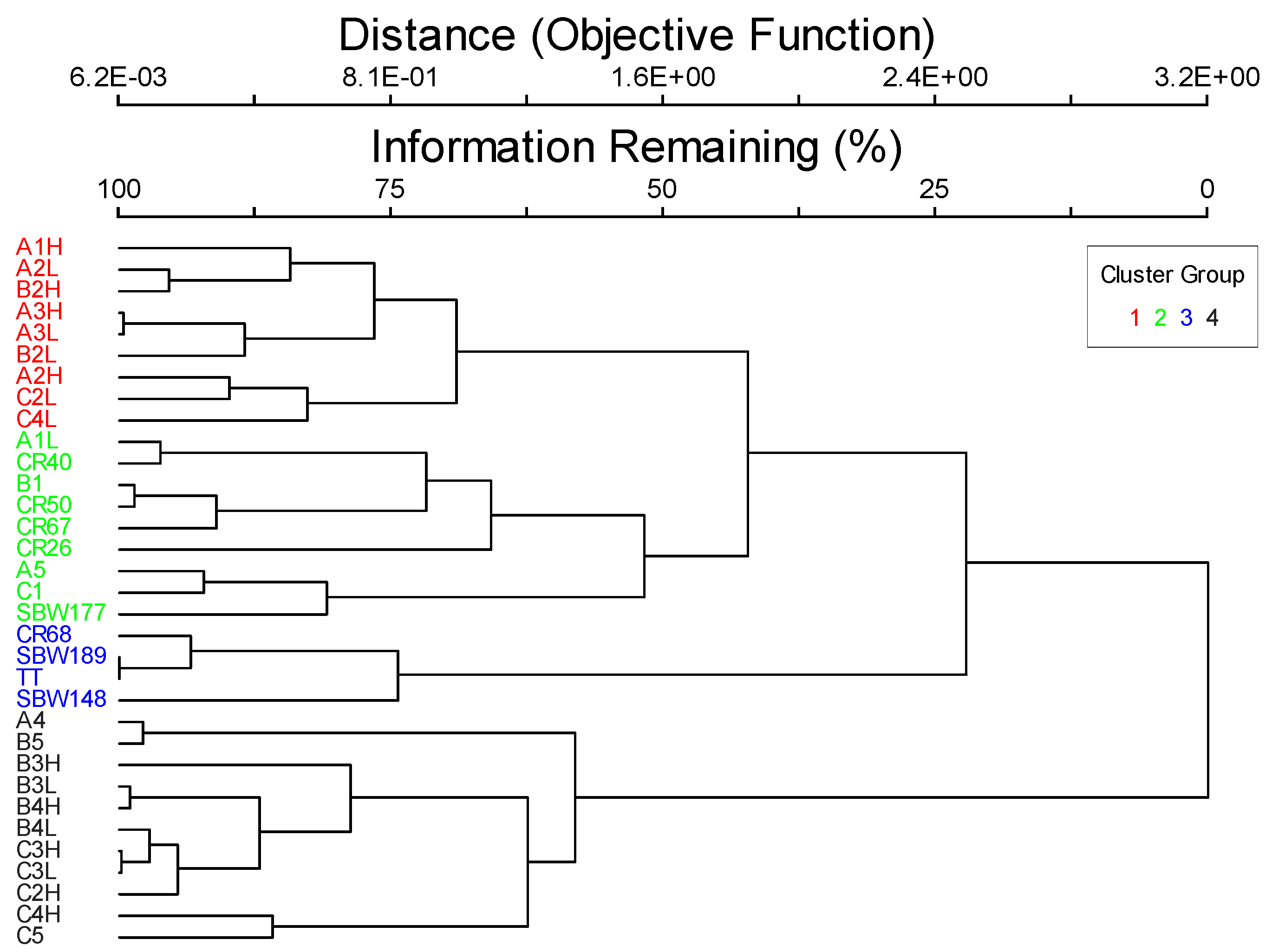
The biotic component consisted of benthic biota with the majority of it attached to the rock substrate. The exception to this was sea urchins that are mobile, but slow enough to still be technically considered attached [3]. Hard corals were present, but were not substantial reef builders, so the biotic class was assigned to faunal bed. The cluster analysis produced four groups of sites with differing benthic communities (Figure 2). However, these groupings were not significantly related to geoforms, substrates, water column components, or any of the CMECS modifiers. The factors influencing the differences between the four taxa cluster groups appear to be much more complicated. Therefore, the whole study area was grouped and classified together. Dominant taxa were sponges, followed by hard corals, brown algae, and red algae. Hard corals were recorded at 90.9% of the sites and sponges at 87.9% of the sites. Within the biotic group of diverse colonizers, I assigned the biotic community as sponge and hard coral colonizers with a co-occurring element of benthic macroalgae (Table 2). This classification was the most applicable to all the sites surveyed within the region.
The results of the species indicator analysis using the four clusters identified in Figure 2 are displayed in Table 4 and Table 5. Groups 1 and 4 had the highest richness that included all the taxa in Table 1, while group 3 consisted of four taxa (Table 4), but also only included four sites (Figure 2). Group 1 was composed of the most indicator species of the four cluster groups (Table 4) and the percent cover of two of those taxa, bivalves, and bryozoans, were significant indicators (Table 5). Group 2 did not have any significant indicator taxa at the p < 0.05 level, but sea urchins and sponges were significant at the p < 0.10 level (Table 5). For group 3, the significant taxon was red algae, and group 4’s indicator taxon was brown algae (Table 5).
The species indicators for each cluster group were generally not significantly correlated to geoforms or substrates, which made it difficult to fit them into the CMECS hierarchical framework (Table 6, and see Kingon [14]). For group 3, red algae was positively correlated with rock percent cover surveyed during the dives but no other geologic variable could be used to differentiate the other three cluster groups (Table 6). Relationships with location, depth, temperature, and water clarity were more common, but even these did not reveal distinct patterns between the cluster groups. Therefore, all the sites were grouped together based on the common occurrences of sponges, hard corals, and macroalgae for the CMECS classification.
4. Discussion
The CMECS works well for the broad-scale classifications and ameliorates mapping, understanding, and management of coastal and marine habitats. Each site, cluster group, and the entire study area can easily be assigned to the classes within the CMECS biogeographic and aquatic settings. It is also possible to classify them using the top tiers of each of the four components, but as you go down the hierarchy, the classification becomes more difficult. The main reasons for these challenges are due to the lack of guidance on how to address variable temporal data, habitat heterogeneity, ecotones, and the different spatial scales that data are collected and related to the biotic components. In addition, I think best practices for data acquisition and application of the CMECS should be developed and included in the standard to serve as a guideline. These best practices would facilitate data comparisons through time and between sites to help evaluate management measures. The problems identified in this study will likely be common issues encountered when the CMECS is applied in other regions and past research, discussed below, has found similar concerns. When these issues, expounded upon in the following sections, are addressed, the power and usefulness of the CMECS will be vastly improved.
4.1. Temporal Scale
For this study, seasonal temporal data were collected; however, it is not clear how to incorporate temporal data into the CMECS classification, especially when it is highly variable. For example, within the water column component, the temperature subcomponents are not applicable for the temperate climate of the Northern Gulf of Mexico. Temperatures ranged from the 11.9 °C to 30.4 °C during the study period, covering several CMECS temperature regimes, from cool to hot water (Table 3). The CMECS does not provide a methodology for how to assign a wide range of water temperatures to a single appropriate category when you collect temporal data. It is not clear whether the temperatures should be assigned to as many classes of water temperature as were encountered or if the temperature data should be averaged so it fits into one class. A standardized methodology for how to account for seasonal temperature variability needs development. A simple solution may be to create a mixed temperature class, but then you may lose the level of detail in the available data. It is likely the need to account for broad temperature ranges will be an issue for other seasonal studies performed in regions with similar climate variability or surveys performed in shallower waters where temperatures may vary seasonally, or even daily. Temperatures can greatly affect the communities present and an area sampled and classified during the winter may have a drastically different community than the same area sampled in the summer [17,18]. Data from either of these seasons on their own would be straightforward to assign CMECS classes; the issues arise when temporal data are collected and the thresholds within a class are crossed. Data could be grouped by season and separate CMECS classifications could be created for each season, but then an understanding of the area over broader temporal scales becomes more difficult. The CMECS claims to be without strict scales but, at the same time, does not contain a means for addressing multiple time scales.
This is not only apparent when dealing with temperature data but also when assigning hydroforms. Currents, waves and fronts operate at a variety of temporal scales and it was not clear how to classify these. Should hydroforms be assigned if they are known to occur in the area or only if they occurred during the study period? If only during the study period, how do you assign the frequency and degree of their effects if those data are available? In estuaries and coastal environments, salinity ranges can vary greatly and the subcomponent classes, again, do not include a mixed class or a way to account for this temporal variability [19].
Challenges were also encountered when dealing with organisms with seasonal occurrences, such as algae. Some species of macroalgae found in the study area tend to grow in the warmer months, while others dominate during the colder seasons, but using the CMECS it was not possible to show these changes. Fishes were not included in this study, but high variability has been observed with different fish species utilizing these habitats at different times of year [17]. I did not find a method within the CMECS to adequately address these temporal changes.
4.2. Spatial Scale
In addition to difficulties that arose with temporal scales, I also encountered some spatial scale challenges. The geoform levels and types had to be adjusted to accommodate this study area. The dominant geoform was pavement area, but this geoform can include many other formations beyond flat pavement. Where there is an exposed pavement edge, a ledge can form and this narrow, linear feature usually harbors higher biodiversity and abundances of organisms than the connected flat pavement areas. As currents move the sediments, the ledge can become more exposed and have higher relief even to the point of being deeply undercut. As these undercuts increase in size, the rock is no longer supported at the edges and can break off, forming rubble fields. Currents or older geologic processes can also erode sand channels into flat pavement forming karren, a more complex habitat. On the other hand, pavement structures can be covered with sand leaving rock outcrops, thinly covered pavement that can still be colonized, sand sheets, or sand wave fields. Several, and occasionally even all, of these geoforms were present in a very small area (<30 m2). How to account for this using the CMECS was not clear as the standard is to assign a geoform and geoform type at level 1 and a second geoform and type at level 2, if appropriate. There did not seem to be a way to account for the complexity of geoforms present at such fine scales. Keefer et al. [20] also found it difficult to assign CMECS classes when multiple geoforms were present and Carollo et al. [21] noted the CMECS was not inclusive of some important habitat types within the Northern Gulf of Mexico. The latter paper does not include the geoforms identified in this paper: pavement area and outcrop that are present and quite extensive in the eastern region of the Northern Gulf of Mexico [21].
This study area is just far enough from shore not to experience major changes from freshwater input. It would be extremely difficult to apply the CMECS to one of the nearby estuaries given the temporal challenges already discussed with changing temperatures and salinities, but also when addressing those issues at the different hierarchical spatial scales.
4.3. Habitat Heterogeneity
Within the substrate component, two substrate classes were present: sand and rock. These were accounted for by using the CMECS co-occurring element modifier, but it was unclear which substrate should be assigned as the “primary” substrate and which should be the co-occurring element. This was especially challenging as percent covers of these two substrate classes varied extensively across sites, with some sites having only 5% exposed rock substrate and others having up to 76% rock from the fine-scale dive surveys. Using the broader-scale sidescan imagery (~400 km2) even less of the area was designated as rock substrate (3–57%). The CMECS guideline for assignment into the rock substrate class was greater than 50% cover, which only some of the dive sites exemplified, and even fewer of the acoustically-mapped areas demonstrated. The rock substrate, however, provides the structure for the biotic components to attach and even when very little is exposed it is still the most important component of the substrate for hardbottom communities. In this case study, a 50% threshold for rock percent cover at either scale is not ecologically relevant, but assignment to the rock class was very important. If the CMECS rules were followed, very few of the sites would be assigned as rock substrate and this could have negative management implications as these rock substrates are likely functioning as essential fish habitat for many fisheries species and can harbor high biodiversity. The mere fact that rock substrate exists should warrant its classification given the increased habitat complexity that is gained by its presence and the changes in communities that will occur where rock substrate exists. I recommend any percentage of rock substrate should be included when applying the CMECS.
When assigning classes in the biotic component, additional difficulties were encountered and modifications required. In the Northern Gulf of Mexico, hard corals are not reef forming, but are one of the dominant taxa found on rock substrate. Hard corals seem to be absent from the classification outside of reef biota which states that “colonizing organisms must be judged to be sufficiently abundant to construct identifiable biogenic substrates” [3], which is unlikely to be the case for the corals encountered in this study. To accommodate for dominance but not in the reef building sense, the biotic community: sponge/hard coral colonizers was created within the faunal bed biotic class, subclass: attached fauna, group: diverse colonizers. It was unexpected that sponge and non-reef building coral communities were absent from the CMECS given their known distribution and importance, particularly in the deep sea [22]. Macroalgae were also dominant taxa at many of the sites; however, they are included in a different biotic class. It is not apparent how to combine biotic components across classes other than stating a co-occurring element, but this method can be misleading. The choice to assign the study area as a faunal bed or aquatic vegetation bed was difficult as one assumes the chosen classification has more significance than a co-occurring element. There is no overlap in the CMECS hierarchies for instances like this, but there should be. Many marine habitats are heterogeneous, particularly the ones in this study area, and assigning co-occurring elements does not provide an accurate depiction of what exists. As mentioned earlier, the dominance of benthic macroalgae is also often seasonal and it is unclear how to annotate that in the standard. Ansari et al. [23] used CMECS to classify habitats in the Persian Gulf, and they found it difficult to account for species diversity and seasonal variations as well.
Apart from the dominant taxa, other rarer species can be indicator species for particular habitats regardless of their abundance. For instance, the dominant species across this study area were sponges, hard corals, and macroalgae, but four distinct communities were identified using cluster analysis (Figure 2). Some of the less abundant taxa present within each cluster were identified as indicator species for those communities. There is no way to address the indicator species or other important taxa in the community using the CMECS. Guarinello et al. [5] also found this to be an issue when they wanted to address sea star predator abundance levels on the mussel reefs they classified.
The common and generally top tier divisions into geologic, biogenic, and anthropogenic classes were difficult to combine when overlap existed. The majority of the sites had geoforms and substrates of geologic origin confirmed via analyzed rock samples, however, for a couple sites, the rock samples turned out to be biogenic structures. These biogenic structures may not be the dominant geoform or substrate at those sites but how to assign different origin classes is not very clear and it may not be possible in the current CMECS [5]. This could be even more problematic in nearby areas that include artificial reefs, pavement areas, and potential biogenic structures [18].
As you reach the bottom of the hierarchy in each CMECS component, the classes provided do not address the habitat heterogeneity and complexities often encountered at these finer scales and ways to better classify habitats using higher resolution data should be developed [24,25]. Keefer et al. [20] found issues with the CMECS when trying to incorporate finer resolution spatial and temporal scales. “The complex interactions over time and space between abiotic and biotic processes often result in ecological boundaries that do not necessarily correspond with boundaries derived using physical or chemical surrogates.” [20]. In concordance with Keefer et al. [20], the CMECS needs more mixed and transitional categories in the standard for each component and at every hierarchical scale to account for heterogeneous areas and transition zones. Habitats are often complex and variable and not a direct result of the substrate, geoform, or water column characteristics present [9,26].
4.4. Ecotones and Seascape Metrics
The current CMECS hierarchy does not appear to have a means for classifying the transition zones that often occur along habitat edges [5]. These ecotones can range from sharp boundaries, such as the ledges mentioned above, to very broad and gradually changing areas [24]. Ecotones are important areas that can have increased biodiversity and greater abundances of organisms [24,27]. As discovered in this study, biological communities are not likely to adhere to the boundaries identified between geoforms, substrate types, or water column properties and the CMECS should have a means for classifying communities that do not follow these boundaries [27,28]. In addition to habitat edges, biotic components can be related to other seascape metrics [14], or parameters outside of those included in the CMECS, such as rugosity, or even location (latitude/longitude), but under the current CMECS, there does not appear to be a way to incorporate seascape metrics or these other data.
4.5. Data Acquisition
Methods should be developed on how best to collect data applicable to the CMECS classification. The intent was for all data to be able to be incorporated into the CMECS but, at the moment, it does not work that way. Therefore, to help standardize the process and allow for more meaningful spatial and temporal comparisons, some guidelines for data collection should be developed. For example, common divisions within the CMECS classes are geologic, biologic, or anthropogenic; however, when researchers collect data, they do not typically stratify habitats in this manner, but could if that were put in a guideline. Stratifying surveys based on the CMECS classes would make its application much easier.
In addition, data should be collected that will provide the information needed to classify features appropriately. For example, I did not use the macroalgae groups for this classification because I did not collect data on growth morphology, and that was the first level of classification for macroalgae. During this study’s dive surveys, macroalgae were assigned based on their phyla, which is more scientifically intuitive than by growth form. I, therefore, suggest using an initial division of macroalgae into the three main phyla: Chlorophyta (green algae), Ochrophyta/Class Phaeophyceae (brown algae), and Rhodophyta (red algae). Then, further classifications could be applied into lower taxonomic levels ending with species and as an alternative based on growth morphology. Most of the algae encountered for this study would probably fit into the leathery/leafy algal bed group, but some of the algae were filamentous, while others were more sheet-like. Grouping them by growth form does not show the differences seen between red algae and brown algae across the study area as their growth forms were often similar, but red algae were more dominant at the western sites and brown algae at the eastern sites with clearer water. Once these algal hierarchies are improved in the CMECS then appropriate survey guidelines can be recommended.
CMECS should also provide more instruction on how to apply their classification system because the results can vary depending on the approach taken [29,30]. If the classification is to be standardized, then a common methodology for assigning hierarchical classes and at what scale should be developed [9]. As it is, the lack of scale in the standard can make it difficult to use and where and how to insert modifiers is also poorly demonstrated [5]. The classification system modified from the CMECS by Guarinello et al. [5] addressed some of these CMECS shortcomings and I think it has more potential for adequately classifying the fine-scale and heterogeneous habitats. Guarinello et al. [5] used several of the same broad-scale classifications in the CMECS but, at the fine-scale, allowed for very detailed entry of both quantitative and qualitative data over multiple sample periods, i.e., you can enter data from three consecutive years and include the densities of multiple species, their percent covers, etc., as well as all the corresponding environmental data and most other details recorded during the study. The format used by Guarinello et al. allows classification of individual sites according to a multitude of parameters and at a variety of spatial and temporal scales [5]. Incorporating these changes into the CMECS would greatly improve it by making maps in different areas and through time comparable. Being able to make these types of comparisons can aid in developing, monitoring, and determining effective marine and coastal management [22].
4.6. Combining Biotic and Abiotic
In this case study, the biotic components did not align with the abiotic, so the question becomes, is it better to classify based on abiotic or biotic characteristics or to assign weights or hierarchies to each [20]? The answer to this question varies depending on the objectives of a study and, thus, makes it difficult to apply a consistent, repeatable classification standard; however, it should still be attempted. The CMECS was developed in order to attempt to include data from almost any type of study and, to many degrees, this is accomplished, especially at the top levels of the hierarchy. Where the CMECS falls short is at the fine-scale and detailed levels of the classification. The relationships between the abiotic and biotic features of a habitat are often difficult to establish and more effort should be put into understanding these habitat complexities rather than trying to simplify them into classes that are not meaningful or relevant [26]. Until then, classes at the lower tiers should be more flexible to allow for the intricacies of each detailed study.
Shumchenia and King [29] showed that a bottom-up approach worked better for classifying habitats than a top-down approach. Top-down generally uses broad-scale remote sensing to map an area and then minimal samples are collected to characterize each class determined from the maps, but this inherently implies that habitats are tied to certain geologic features of the seafloor [29]. Other environmental and ecological characteristics are not taken into consideration and are often important in determining the distribution of biotic communities [29]. Shumchenia and King [29] also did not observe a simple relationship between the biotic groups and the broad scale acoustic classes (silt and sand); linkages to abiotic features were at fine scales. This study only found relationships with the acoustic data for bivalves and sea urchins, but not the other indicator species for those clusters; most of the influencing factors appeared to be at finer scales as well (Table 6). It was difficult for both this study and Shumchenia and King [29] to include the details in CMECS, but inclusion of those details may not be needed at scales the CMECS intended for regional or national management and conservation purposes [29].
4.7. Future Work
Future options for this study’s results and for other similar studies could be to try to classify individual sites separately or to implement the modified system developed by Guarinello et al. [5] and apply it to each site or cluster group. The high variability seen within and between sites in this study indicates that finer scale sampling may be needed. Sampling directed towards particular geoforms at a site may reveal distinct biotic associations with them. Taxonomic groups were used for this study rather than individual species and those taxa groupings could be obscuring more definitive associations each species may have with its physical environment, which could clear up some of the classifications. More work at that level of detail is recommended to see if the CMECS would work better.
5. Conclusions
Overall the CMECS is a very powerful classification tool that is improving our understanding and management of coastal and marine habitats in the U.S. and beyond. However, improvements are needed. The CMECS works well when habitats are fairly homogenous over broad spatial scales [5]. It also likely performs adequately for studies occurring over narrow time scales or synchronously each year. When habitats are heterogeneous at finer scales and seasonal data are incorporated, the relationships between the biotic and abiotic components become complex and distinct classifications based on substrate or geoform type are often not possible. The modifiers can be used, but do not represent the complexities accurately. I think it is important to have a national classification standard and to fit marine habitat data into it at the finest scale possible. When incorporating finer scale data, the dominant taxa may not be what makes sites similar and, in these cases, indicator species could be much more important and informative to use. I think FGDC could easily incorporate these changes into the CMECS.
As with other established classification systems, modifications are common, particularly during the preliminary phases of development. As people use classification systems, make discoveries, and develop new technology, some of the initial classifications may no longer be applicable and additional classes will need to be added. FGDC seems to understand this and they have included provisions in the CMECS manual for modifications [3]. Marine habitat classification is not an easy task due to the complexities of habitats and the processes and patterns operating three-dimensionally and at various geographic and temporal scales. Revisions to address the challenges encountered will greatly enhance the utility of the CMECS.
Acknowledgments
This work would not have been possible without guidance and assistance from the faculty, staff, and students at the Florida State University (FSU) Coastal and Marine Lab; particularly, Chris Koenig and Felicia Coleman, field assistants: Stephanie White, Jennifer Schellinger, Bob Ellis, Chris Stallings, Chris Peters, Justin Lewis, Chelsie Counsell, Sonja Bridges, Zach Boudreau, and Donnie McClain; and visiting researchers who made time for me to collect data during their research trips: Don DeMaria, Christian Boniface, and Peter Auster. Many thanks to Kathy Scanlon at the United States Geological Survey in Woods Hole, Massachusetts and Harley Means at the Florida Geological Survey (FGS) for analysing the rock samples and providing their geological expertise. Also at FGS, thank you Dan Phelps for sharing your office space, time, and a computer to analyse all the sidescan sonar data. Within the FSU Center for Ocean-Atmospheric Prediction Studies, Austin Todd, Steve Morey, and Dmitry Dukhovskoy provided oceanographic knowledge on the Gulf of Mexico to guide the CMECS hydroform classification. My dissertation advisor at FSU, Tingting Zhao, and the rest of my dissertation committee, Xiaojun Yang, Markus Huettel, Chris Uejio, and Tony Stallins, greatly assisted with project planning and execution, as well as editing. Information on local hardbottom habitats and sidescan sonar was gleaned from Chris Gardner, Doug DeVries, and Patrick Raley at the National Marine Fisheries Service Lab in Panama City, Florida. Field work for this study was partially funded through the Northern Gulf Institute via a Gulf of Mexico Research Initiative grant, “Impact of crude oil on coastal and ocean environments of the West Florida Shelf and Big Bend Region from the shoreline to the continental shelf edge” (PIs, Eric Chassignet and Felicia Coleman: 191001-3066811-03/T) and via funds from BP and the U.S. National Oceanic and Atmospheric Association (191001-363558-01).
Conflicts of Interest
The author declares no conflict of interest.
References
- Anderson, J.R.; Hardy, E.E.; Roach, J.T. A Land Use and Land Cover Classification System for Use with Remote Sensor Data; U.S. Geological Survey Cire: Reston, VA, USA, 1972.
- Anderson, J.R.; Hardy, E.E.; Roach, J.T.; Witmer, R.E. A Land Use Classification System for Use with Remote-Sensor Data; U.S. Geological Survey Professional Paper 964; U.S. Geological Survey: Reston, VA, USA, 1976.
- Federal Geographic Data Committee (FGDC). Coastal and Marine Ecological Classification Standard. Available online: https://www.fgdc.gov/standards/projects/cmecs-folder/CMECS_Version_06-2012_FINAL.pdf (accessed on 12 January 2018).
- Davies, C.E.; Moss, D.; Hill, M.O. EUNIS Habitat Classification Revised 2004. Available online: https://www.eea.europa.eu/data-and-maps/data/eunis-habitat-classification/documentation/eunis-2004-report.pdf/download (accessed on 12 January 2018).
- Guarinello, M.L.; Shumchenia, E.J.; King, J.W. Marine habitat classification for ecosystem-based management: A proposed hierarchical framework. Environ. Manag. 2010, 45, 793–806. [Google Scholar] [CrossRef] [PubMed]
- Gibbs, A.E.; Cochran, S.A.; Logan, J.B.; Grossman, E.E. Benthic Habitats and Offshore Geological Resources of Kaloko-Honnok–Ohau National Historical Park, Hawai`i. Available online: https://pubs.usgs.gov/sir/2006/5256/sir2006-5256.pdf (accessed on 12 January 2018).
- Greene, H.G.; Yoklavich, M.M.; Starr, R.M.; O’Connell, V.M.; Wakefield, W.W.; Sullivan, D.E.; McRea, J.E.; Cailliet, G.M. A classification scheme for deep seafloor habitats. Oceanol. Acta 1999, 22, 663–678. [Google Scholar] [CrossRef]
- Mumby, P.J.; Harborne, A.R. Development of a systematic classification scheme of marine habitats to facilitate regional management and mapping of Caribbean coral reefs. Biol. Conserv. 1999, 88, 155–163. [Google Scholar] [CrossRef]
- Auster, P.J.; Heinonen, K.B.; Witharana, C.; McKee, M. A Habitat Classification Scheme for the Long Island Sound Region. Available online: http://longislandsoundstudy.net/wp-content/uploads/2010/02/Auster-et-al_EPA-Final-Technical-Report_Habitat-Classification_June-091.pdf (accessed on 12 January 2018).
- Briones, E.E. Current knowledge of benthic communities in the Gulf of Mexico. In Environmental Analysis of the Gulf of Mexico; Withers, K., Nippers, M., Eds.; Texas A&M University: Corpus Christi, TX, USA, 2003. [Google Scholar]
- Kendall, M.S.; Buja, K.R.; Christensen, J.D.; Kruer, C.R.; Monaco, M.E. The seascape approach to coral ecosystem mapping: An integral component of understanding the habitat utilization patterns of reef fish. Bull. Mar. Sci. 2004, 75, 225–237. [Google Scholar]
- Galtsoff, P.S. Gulf of Mexico: Its Origin, Waters, and Marine Life; Fishery Bulletin of the Fish and Wildlife Service: Washington, DC, USA, 1954. [Google Scholar]
- Kendall, M.S.; Jensen, O.P.; Alexander, C.; Field, D.; McFall, G.; Bohne, R.; Monaco, M.E. Benthic mapping using sonar, video transects, and an innovative approach to accuracy assessment: A characterization of bottom features in the Georgia Bight. J. Coast. Res. 2005, 21, 1154–1165. [Google Scholar] [CrossRef]
- Kingon, K.C. Mapping, Classification, and Spatial Variation of Hardbottom Habitats in the Northeastern Gulf of Mexico. Ph.D. Thesis, Florida State University, Tallahassee, FL, USA, 2013. [Google Scholar]
- Peck, J.E. Multivariate Analysis for Community Ecologists: Step-by-Step Using PC-ORD. Available online: https://www.researchgate.net/publication/285753955_Multivariate_Analysis_for_Community_Ecologists_Stepby-_Step_using_PC-ORD (accessed on 12 January 2018).
- Schellinger, J. Hardbottom Sessile Macroinvertebrate Communities of the Apalachee Bay Region of Florida’s Northeastern Gulf of Mexico. Master’s Thesis, Florida State University, Tallahassee, FL, USA, 2013. [Google Scholar]
- Cheney, D.P.; Dyer, J.P. Deep-water benthic algae of the Florida Middle Ground. Mar. Biol. 1974, 27, 185–190. [Google Scholar] [CrossRef]
- Kingon, K.C.; Koenig, C.C.; Brooke, S.; Stallings, C.D.; Wall, K.; Sandon, C. Do artificial reefs sustain communities similar to nearby natural reefs? A seasonal study in the northeastern Gulf of Mexico. In Proceedings of the 67th Annual Meeting of the Gulf and Caribbean Fisheries Institute, Christ Church, Barbados, 3–7 November 2015. [Google Scholar]
- Cochrane, G.R.; Dethier, M.N.; Hodson, T.O.; Kull, K.J.; Golden, N.E.; Ritchie, A.C.; Moegling, C.H.; Pacunski, R.E. Salish Seas Map Series—Admirality Inlet; Geological Survey Open-File Report 2015-1073; U.S. Geological Survey: Reston, VA, USA, 2015.
- Keefer, M.L.; Peery, C.A.; Wright, N.; Daigle, W.R.; Caudill, C.C.; Clabough, T.S.; Griffith, D.W.; Zacharias, M.A. Evaluating the NOAA coastal and marine ecological classification standard in estuarine systems: A Columbia River estuary case study. Estuar. Coast. Shelf Sci. 2008, 78, 89–106. [Google Scholar] [CrossRef]
- Carollo, C.; Allee, R.J.; Yoskowitz, D.W. Linking the Coastal and Marine Ecological Classification Standard (CMECS) to ecosystem services: An application to the US Gulf of Mexico. Int. J. Biodivers. Sci. Ecosyst. Ser. Manag. 2013, 9, 249–256. [Google Scholar] [CrossRef]
- Davies, J.S.; Stewart, H.A.; Narayanaswamy, B.E.; Jacobs, C.; Spicer, J.; Golding, N.; Howell, K.L. Benthic assemblages of the Anton Dohrn Seamount (NE Atlantic): Defining deep-sea biotopes to support habitat mapping and management efforts with a focus on vulnerable marine ecosystems. PLoS ONE 2015, 10, 1–33. [Google Scholar] [CrossRef] [PubMed]
- Ansari, Z.; Seyfabadi, J.; Owfi, F.; Rahimi, M.; Allee, R. Ecological classification of southern intertidal zones of Qeshm Island, based on CMECS model. Iran. J. Fish. Sci. 2014, 13, 1–19. [Google Scholar]
- Zajac, R.N.; Lewis, R.S.; Poppe, L.J.; Twichell, D.C.; Vozarik, J.; DiGiacomo-Cohen, M.L. Responses of infaunal populations to benthoscape structure and the potential importance of transition zones. Limnol. Oceanogr. 2003, 48, 829–842. [Google Scholar] [CrossRef]
- Zajac, R.N. Macrobenthic biodiversity and sea floor landscape structure. J. Exp. Mar. Biol. Ecol. 2008, 366, 198–203. [Google Scholar] [CrossRef]
- Diaz, R.J.; Solan, M.; Valente, R.M. A review of approaches for classifying benthic habitats and evaluating habitat quality. J. Environ. Manag. 2004, 73, 165–181. [Google Scholar] [CrossRef] [PubMed]
- Zajac, R.N. Challenges in marine, soft-sediment benthoscape ecology. Landsc. Ecol. 2008, 23, 7–18. [Google Scholar] [CrossRef]
- Hewitt, J.E.; Thrush, S.E.; Legendre, P.; Funnell, G.A.; Ellis, J.; Morrison, M. Mapping of marine soft-sediment communities: Integrated sampling for ecological interpretation. Ecol. Appl. 2004, 14, 1203–1216. [Google Scholar] [CrossRef]
- Shumchenia, E.J.; King, J.W. Comparison of methods for integrating biological and physical data for marine habitat mapping and classification. Coast. Shelf Res. 2010, 30, 1717–1729. [Google Scholar] [CrossRef]
- Cook, R.R.; Auster, P.J. A Bioregional Classification of the Continental Shelf of Northeastern North America for Conservation Analysis and Planning Based on Representation; Marine Sanctuaries Conservation Series NMSP-0; NOAA’s National Ocean Service: Ginsen, MD, USA, 2007.
Figure 1.
Study area showing site names and locations as black squares approximately to scale representing the 400 m × 400 m areas mapped using the Humminbird 997c side imaging system (Humminbird, Eufaula, AL, USA). Light gray lines represent bathymetry contours.
Figure 1.
Study area showing site names and locations as black squares approximately to scale representing the 400 m × 400 m areas mapped using the Humminbird 997c side imaging system (Humminbird, Eufaula, AL, USA). Light gray lines represent bathymetry contours.

Figure 2.
Dendrogram showing the four cluster groups that resulted when the data were separated with 50 percent information remaining.
Figure 2.
Dendrogram showing the four cluster groups that resulted when the data were separated with 50 percent information remaining.

Table 1.
A list of the different taxa groups identified and assigned during the point surveys along the transects.
Table 1.
A list of the different taxa groups identified and assigned during the point surveys along the transects.
| Taxa | |
|---|---|
| brown algae | hard coral |
| red algae | hydroid |
| green algae | gorgonian |
| colonial tunicate | sponge |
| solitary tunicate | bivalve |
| bryozoan | sea urchin |
Table 2.
Classification of the Northeastern Gulf of Mexico nearshore hardbottom habitats using the CMECS.
Table 2.
Classification of the Northeastern Gulf of Mexico nearshore hardbottom habitats using the CMECS.
| Northeastern Gulf of Mexico off Northwest Florida (10–23 m Depths) |
|---|
| Biogeographic Setting |
| Realm: Temperate Northern Atlantic |
| Province: Warm Temperate Northwest Atlantic |
| Ecoregion: Northern Gulf of Mexico |
| Aquatic Setting |
| System: Marine |
| Subsystem: Nearshore |
| Tidal Zone: Subtidal |
| Water Column Component |
| Water Column Layer: Marine Nearshore Lower Water Column |
| Salinity Regime: Euhaline |
| Temperature Regime: Warm |
| Geoform Component |
| Tectonic Setting: Passive Continental Margin |
| Physiographic Setting: Continental Shelf |
| Physiographic Setting: Embayment/Bay |
| Geoform Origin: Geologic |
| Level 1 Geoform: Pavement Area |
| Level 2 Geoform: Ledge |
| Level 2 Geoform: Karren |
| Level 1 Geoform: Outcrop |
| Substrate Component |
| Substrate Origin: Geologic Substrate |
| Substrate Class: Rock Substrate |
| Substrate Subclass: Bedrock (5–76% exposed) |
| Co-occurring Element: Sand (24–88%) |
| Biotic Component |
| Biotic Setting: Benthic/Attached Biota |
| Biotic Class: Faunal Bed |
| Biotic Subclass: Attached Fauna |
| Biotic Group: Diverse Colonizers |
| Biotic Community: Sponge/Hard Coral Colonizers |
| Co-occurring Element: Benthic Macroalgae |
Table 3.
The water column components that exist within the study area at different times.
| Water Column Layer | Salinity Regime | Temperature Regime | Hydroform Class | Hydroform | Hydroform Type |
|---|---|---|---|---|---|
| marine nearshore surface Layer | euhaline water | cool water | current | ekman flow | ekman upwelling |
| marine nearshore upper water Column | moderate water | ekman downwelling | |||
| marine nearshore pycnocline | warm water | inertial current | |||
| marine nearshore lower water column | very warm water | langmuir circulation | |||
| hot water | tidal flow | mixed semi-diurnal tidal flow | |||
| wind-driven current | |||||
| front | coastal upwelling front | ||||
| Tidal Front | |||||
| Wave | Coastally Trapped Wave | Shelf Wave | |||
| Storm Surge |
Table 4.
Results from the indicator species analysis performed in PC-ORD (MjM Software, Gleneden Beach, OR, USA) for the cluster analysis groupings shown in Figure 2. This table shows the indicator values calculated by multiplying the relative abundance and relative frequency values of each taxa to obtain the percent of perfect indication for each cluster group.
| Taxa | Average | Maximum | Maximum Group | Cluster Group Indicator Values (%) | |||
|---|---|---|---|---|---|---|---|
| 1 | 2 | 3 | 4 | ||||
| bivalve | 22 | 86 | 1 | 86 | 0 | 0 | 3 |
| bryozoan | 17 | 57 | 1 | 57 | 4 | 0 | 8 |
| green algae | 13 | 33 | 1 | 33 | 1 | 0 | 19 |
| gorgonian | 8 | 19 | 1 | 19 | 0 | 0 | 11 |
| solitary tunicate | 7 | 24 | 1 | 24 | 1 | 0 | 4 |
| colonial tunicate | 12 | 29 | 2 | 18 | 29 | 0 | 3 |
| sponge | 22 | 37 | 2 | 24 | 37 | 19 | 10 |
| sea urchin | 12 | 38 | 2 | 7 | 38 | 0 | 4 |
| hydroid | 13 | 17 | 3 | 9 | 12 | 17 | 15 |
| red algae | 24 | 80 | 3 | 9 | 2 | 80 | 3 |
| brown algae | 25 | 69 | 4 | 29 | 0 | 0 | 69 |
| hard coral | 24 | 33 | 4 | 24 | 11 | 26 | 33 |
| Averages | 17 | 43 | 28 | 11 | 12 | 15 | |
Table 5.
The results from the species indicator Monte Carlo randomization test using 1000 permutations completed in PC-ORD (MjM Software, Gleneden Beach, OR, USA) for each of the four cluster groups identified in Figure 2. It shows the p-values which indicate when a large proportion of the randomization tests have indicator values higher or equal to the observed indicator value. Only taxa with significant p-values (<0.10) for each cluster group are shown.
| Taxa | Maximum Group | Observed Indicator Value | p |
|---|---|---|---|
| bivalve | 1 | 85.9 | 0.001 |
| bryozoan | 1 | 57.1 | 0.007 |
| sponge | 2 | 36.9 | 0.092 |
| sea urchin | 2 | 37.7 | 0.060 |
| red algae | 3 | 80.4 | 0.001 |
| brown algae | 4 | 69.3 | 0.001 |
Table 6.
The six significant indicator species identified for the four cluster groups (Table 5) were correlated with physical and environmental data for the sites. The significant correlation coefficients between the variables and the indicator species are shown below, highlighted in yellow. This table does not include all the variables that were measured, only the ones significant to the indicator taxa (see Kingon [14] for the others).
| Cluster Group | Group 1 | Group 2 | Group 3 | Group 4 | ||
|---|---|---|---|---|---|---|
| Variables | Bivalve | Bryozoan | Sponge | Sea Urchin | Red Algae | Brown Algae |
| Latitude | 0.452 | 0.256 | 0.145 | −0.130 | 0.257 | −0.024 |
| Longitude | 0.143 | −0.025 | −0.648 | −0.197 | −0.286 | 0.400 |
| Distance to shore | −0.190 | −0.208 | −0.432 | −0.059 | −0.295 | 0.359 |
| Mean depth | −0.451 | −0.211 | 0.062 | 0.102 | −0.174 | −0.125 |
| Rock percent cover | −0.040 | −0.271 | 0.216 | 0.142 | 0.502 | 0.021 |
| Rock type | 0.168 | −0.496 | −0.120 | −0.028 | 0.193 | 0.106 |
| Mean sand depth | 0.067 | 0.384 | 0.041 | 0.121 | −0.150 | −0.057 |
| Thin sand percent cover | 0.081 | −0.020 | −0.100 | −0.350 | −0.234 | 0.026 |
| Mean bottom temperature | 0.083 | 0.114 | 0.553 | 0.046 | 0.408 | −0.037 |
| Mean vertical visibility | 0.042 | −0.125 | −0.456 | −0.236 | −0.168 | 0.462 |
| Mean horizontal visibility | 0.415 | −0.025 | −0.440 | −0.194 | −0.235 | 0.337 |
| Hardbottom percent cover from the acoustic data | 0.252 | 0.123 | −0.226 | −0.414 | −0.013 | 0.285 |
| Video relief | −0.350 | −0.149 | 0.218 | 0.088 | 0.336 | −0.248 |
| Video heterogeneity | −0.139 | −0.520 | 0.093 | 0.120 | 0.309 | −0.200 |
| Geoform from the acoustic data | −0.466 | −0.028 | 0.093 | 0.060 | 0.043 | −0.182 |
| Heterogeneity from the acoustic data | 0.234 | 0.308 | −0.088 | −0.423 | 0.227 | 0.318 |
| Relief from the acoustic data | −0.386 | −0.040 | 0.224 | 0.145 | 0.127 | <−0.001 |
© 2018 by the author. Licensee MDPI, Basel, Switzerland. This article is an open access article distributed under the terms and conditions of the Creative Commons Attribution (CC BY) license (http://creativecommons.org/licenses/by/4.0/).
Share and Cite
MDPI and ACS Style
Kingon, K. Applying the Coastal and Marine Ecological Classification Standard (CMECS) to Nearshore Habitats in the Northeastern Gulf of Mexico. Geosciences 2018, 8, 22. https://doi.org/10.3390/geosciences8010022
AMA Style
Kingon K. Applying the Coastal and Marine Ecological Classification Standard (CMECS) to Nearshore Habitats in the Northeastern Gulf of Mexico. Geosciences. 2018; 8(1):22. https://doi.org/10.3390/geosciences8010022
Chicago/Turabian StyleKingon, Kelly. 2018. "Applying the Coastal and Marine Ecological Classification Standard (CMECS) to Nearshore Habitats in the Northeastern Gulf of Mexico" Geosciences 8, no. 1: 22. https://doi.org/10.3390/geosciences8010022
Note that from the first issue of 2016, this journal uses article numbers instead of page numbers. See further details here.