Pyplis–A Python Software Toolbox for the Analysis of SO2 Camera Images for Emission Rate Retrievals from Point Sources

 , ,
, ,
Abstract
:1. Introduction
- 3D distance retrievals to plume and local terrain features at pixel-level,
- several methods to retrieve plume background radiances,
- cell and DOAS based camera calibration including two independent DOAS FOV search routines,
- cross-correlation and optical flow based plume velocity retrievals,
- histogram based correction for ill-posed optical flow vectors in low-contrast image regions,
- image based correction for the signal dilution effect,
- automated emission rate retrievals along linear plume intersections.
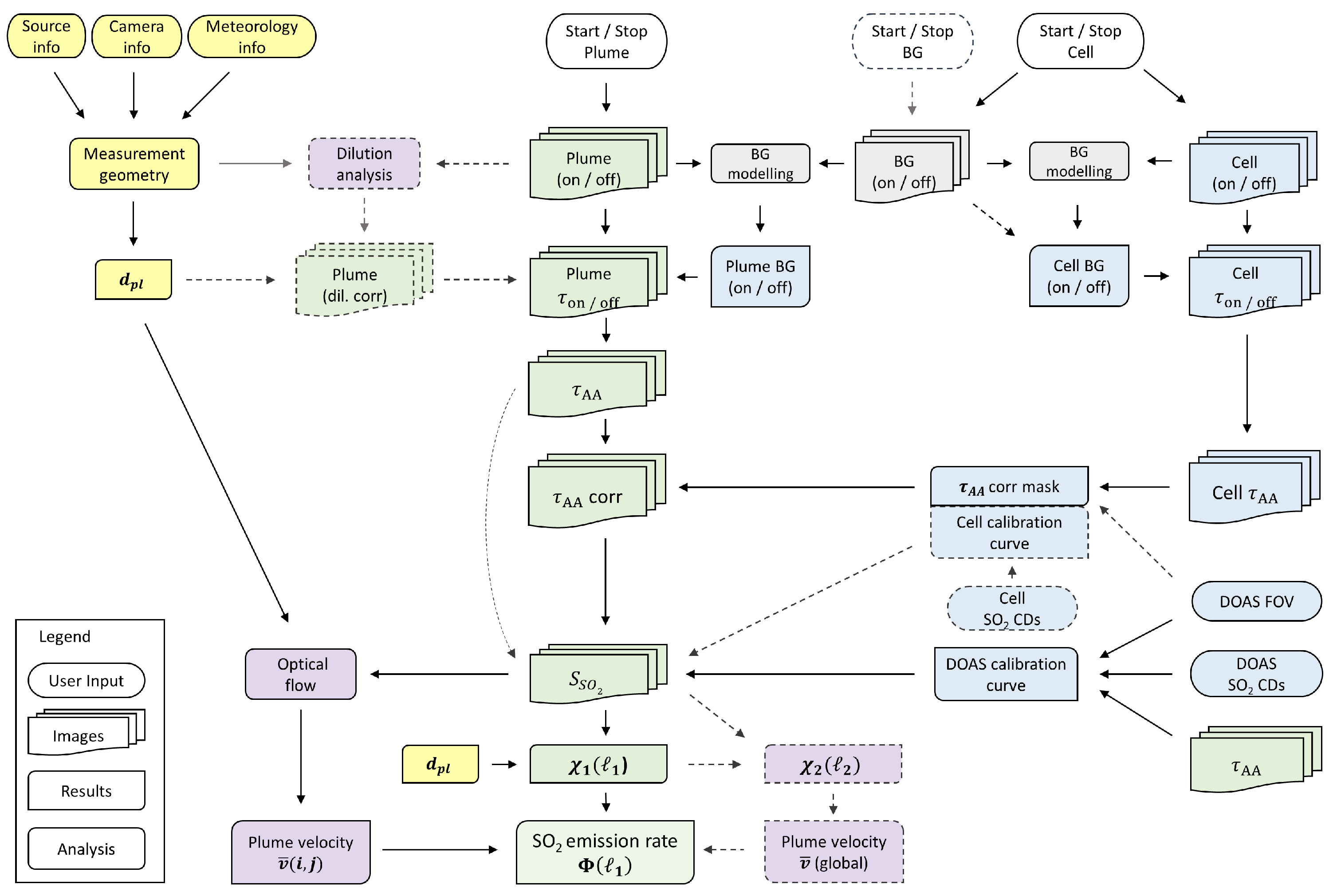
2. Methodology
2.1. UV SO2 Cameras
2.2. Image Analysis—Retrieval of S Images
2.3. Emission Rate Retrieval
2.4. Radiative Transfer Corrections
3. Implementation
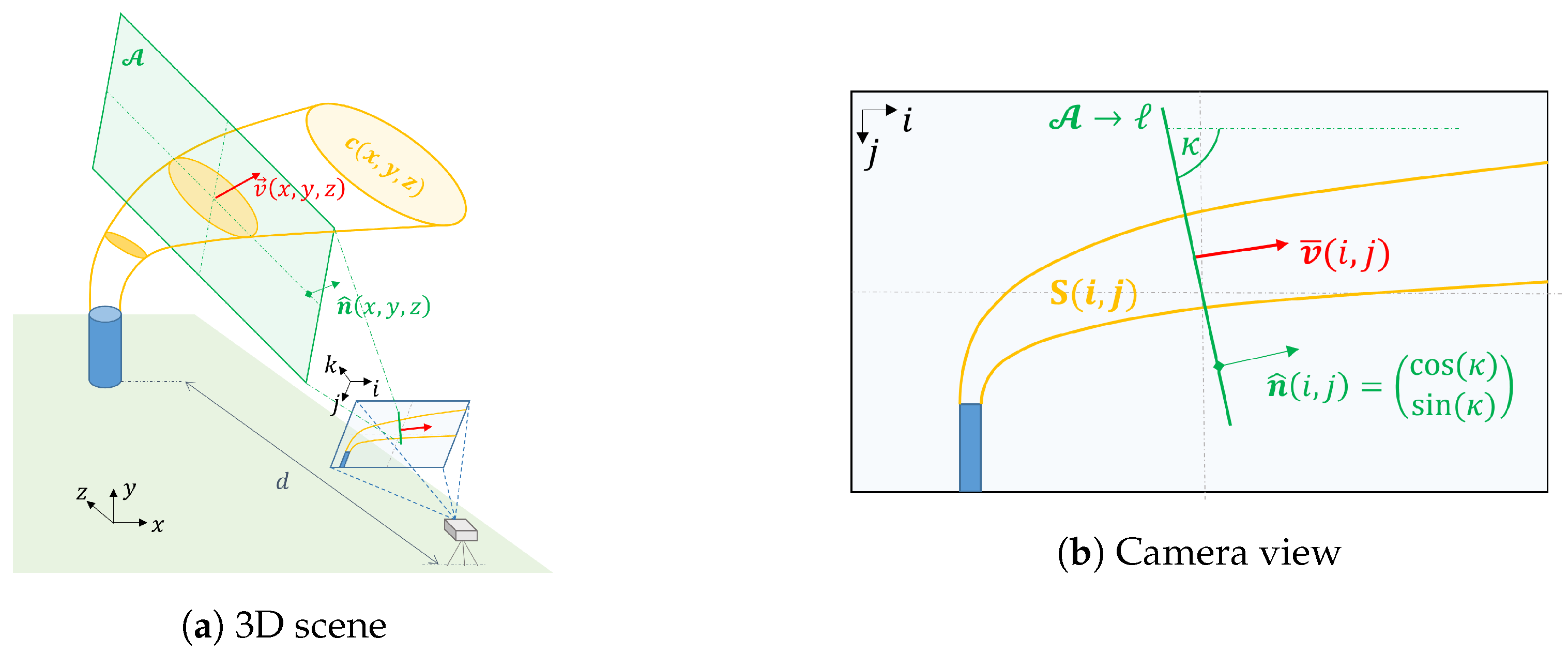
3.1. Geometrical Calculations
3.2. Image Representation and Pre-Processing Routines
3.3. Retrieval of Plume Background Radiances
3.4. Camera Calibration
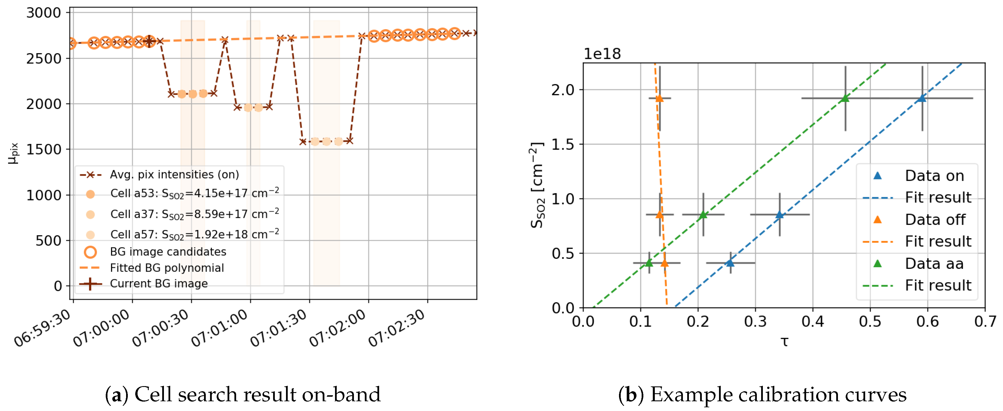
3.4.1. Calibration Using SO2 Cells
3.4.2. Calibration Using DOAS Data
3.4.3. DOAS FOV Search
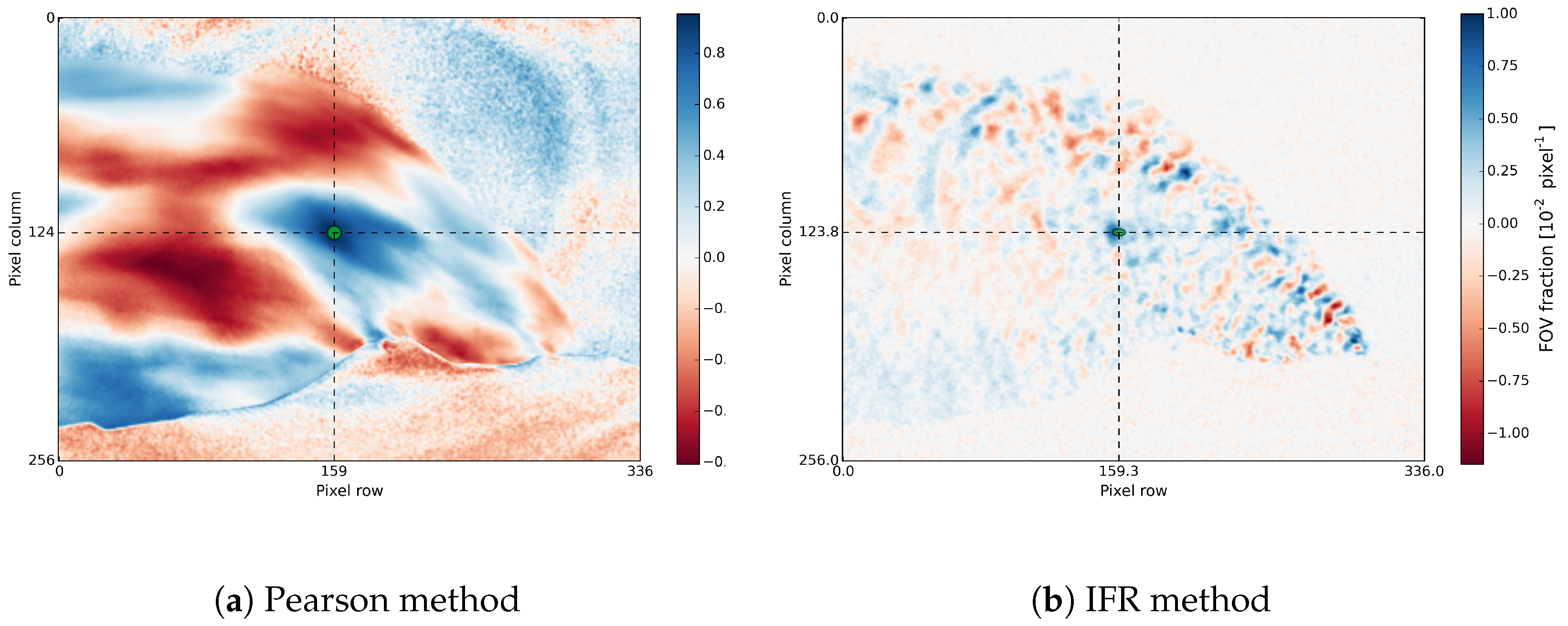
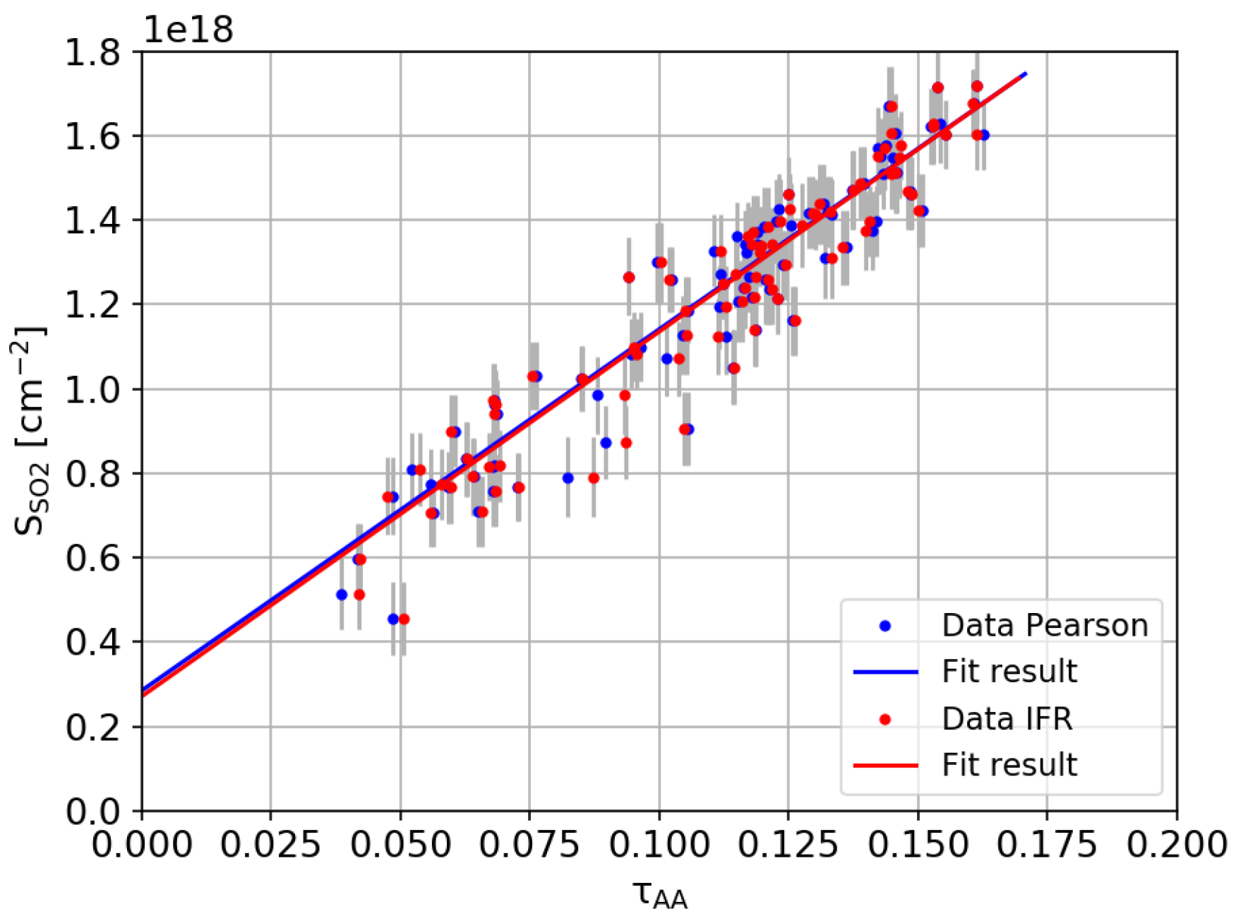
- Pearson routine: this method loops over all image pixels in the AA stack and determines the Pearson correlation coefficient between the corresponding AA time-series () and the DOAS SO2-CD vector (). The method yields a correlation image as shown in Figure 7a, from which the pixel coordinate with highest correlation () is extracted (see also [21]). Assuming a circular FOV shape, the pixel extent of the FOV is estimated around , by iteratively searching the disk radius with highest correlation between the AA and the DOAS time-series.
- In-operation field-of-view retrieval (IFR) routine: this method is based on [30] and uses an inversion algorithm to retrieve the FOV. Position and shape of the FOV is parametrised by fitting a 2D Super-Gaussian to the retrieved FOV distribution (shown in Figure 7b, see Appendix D.2 for details).
3.5. Plume Velocity Analysis
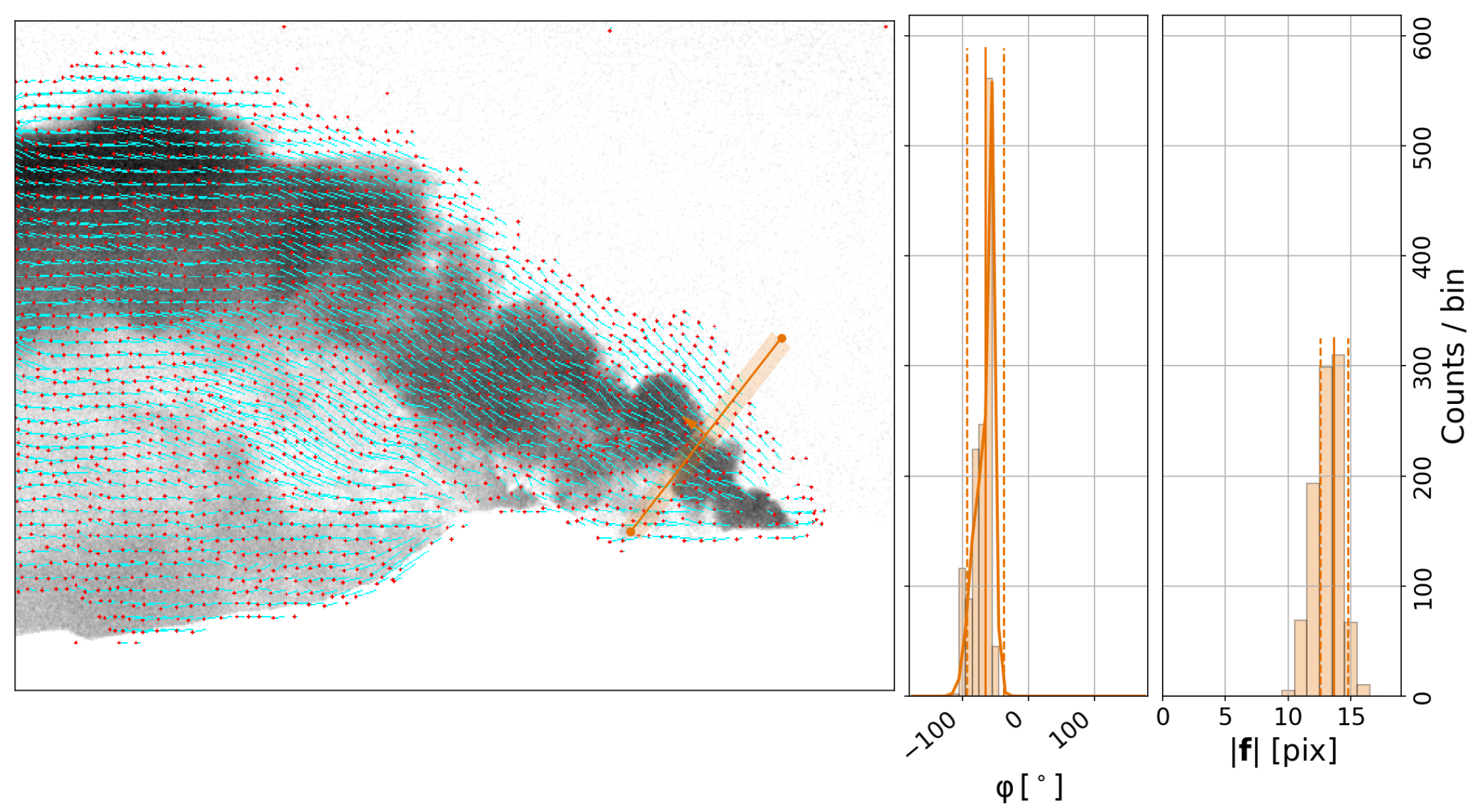
3.5.1. Velocity Retrieval Using the ICA Cross-Correlation Method
3.5.2. Optical Flow Based Velocity Retrievals
3.6. Image Based Signal Dilution Correction
3.7. Emission Rate Retrieval
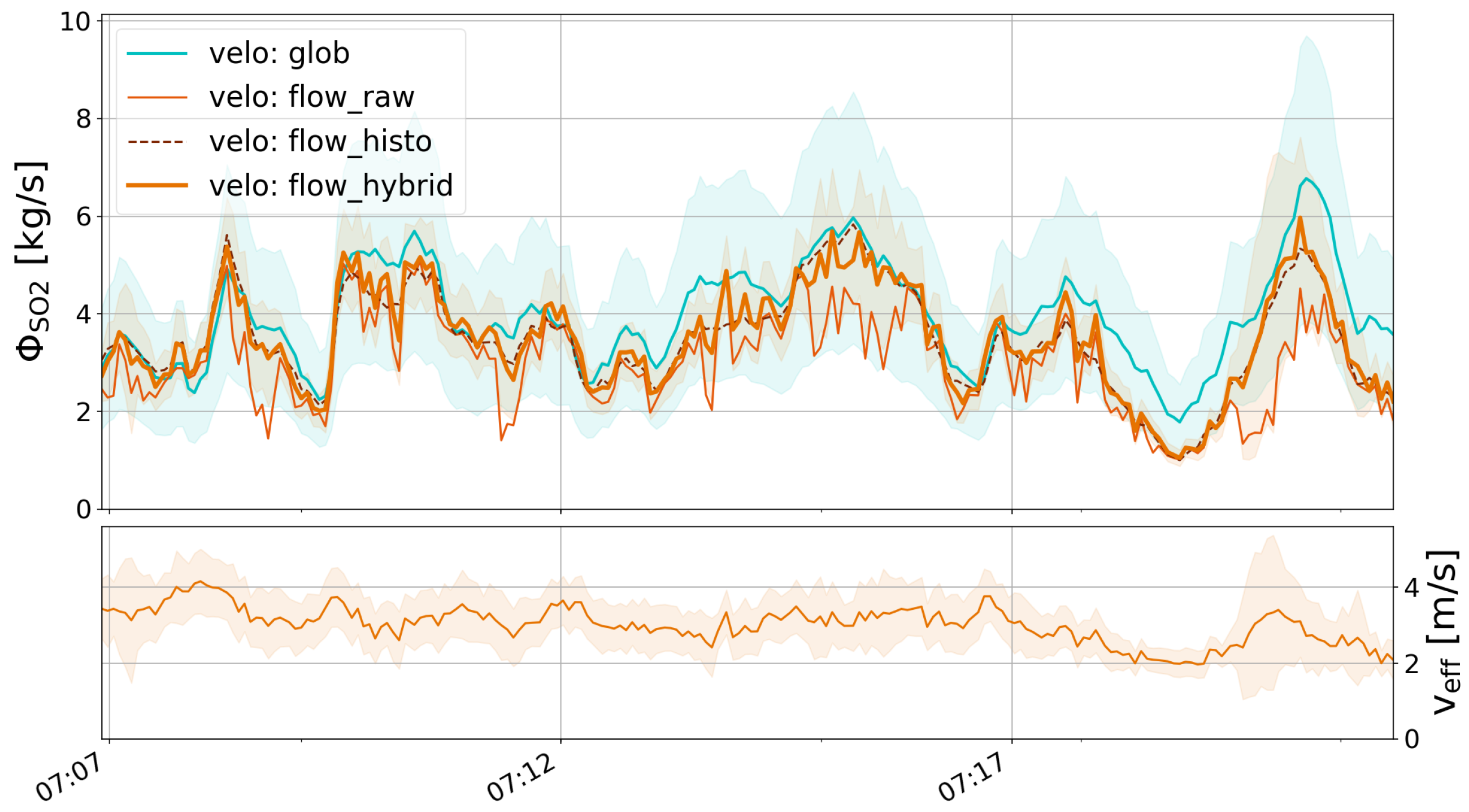
- flow_raw → the raw output of the Farnebäck algorithm is used. This should only be done if it can be assured that the algorithm yields reliable output in the considered plume area (i.e., ROI around the PCS line) and for all images of the time-series.
- flow_histo → performs the histogram post-analysis proposed by [43] (cf. Section 3.5.2). The retrieved local average velocity vector for each PCS line is then used as a velocity estimate for the corresponding retrieval line.
- flow_hybrid → reliable motion vectors from the flow field are used while unreliable ones are identified and replaced based on the histogram post-analysis (see previous point).
Remark on Performance
3.8. Remark on Uncertainties
4. Conclusions
Acknowledgments
Author Contributions
Conflicts of Interest
Abbreviations
| UV | Ultraviolet |
| CD | Column density |
| DOAS | Differential optical absorption spectroscopy |
| FOV | Field of view |
| OD | Optical density |
| AA | SO2 apparent absorbance |
| PCS | Plume cross section |
| ICA | Integrated column amount |
| API | Application programming interface |
| IFR | In-operation field-of-view retrieval |
Appendix A. The Geonum Python library
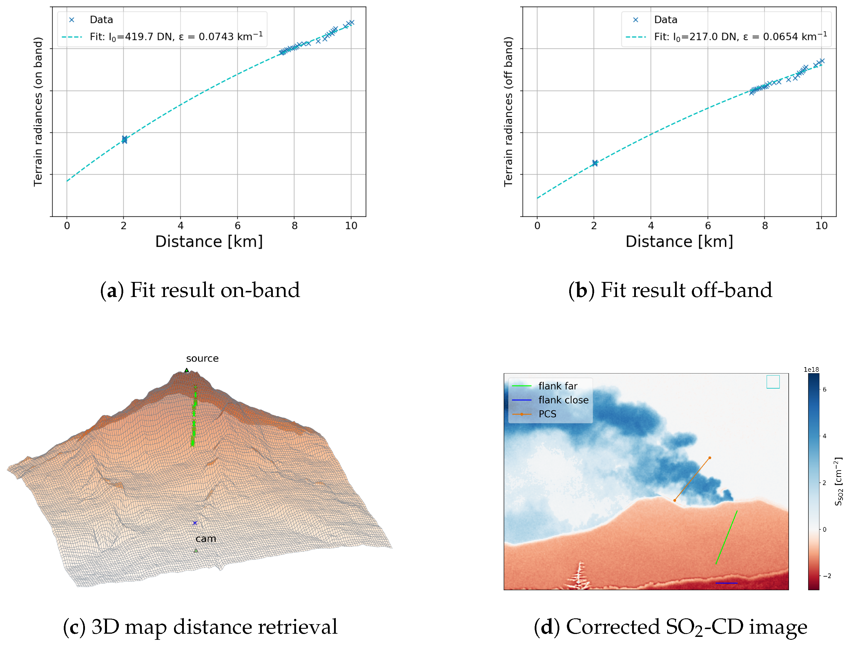
Appendix A.1. Pixel Based Retrieval of Distances to Local Terrain Features
Appendix B. Performance of Typical Analysis Chain
- Image import and dark and offset correction (on and off-band).
- Further image preparation operations (e.g., noise reduction using Gaussian blurring filter, size reduction using Gaussian pyramid).
- Plume background modelling (on, off) and calculation of -image.
- Image calibration (i.e., requires availability of calibration curve).
- Optional: computation of optical flow field.

| Blur | Pyrlevel | Computation Time [s] | ||
|---|---|---|---|---|
| Image Preparation (Steps 1–4) | Optical Flow (Step 5) | Total | ||
| 10 | 0 | 0.350 | 0.823 (70 %) | 1.173 |
| 0 | 0 | 0.188 | 0.813 (81 %) | 1.001 |
| 0 | 1 | 0.205 | 0.202 (50 %) | 0.407 |
| 0 | 2 | 0.203 | 0.103 (34 %) | 0.306 |
Appendix C. Dark and Offset Correction
- Option 1: Modelling of Dark/Offset ImageThe correction is performed based on two dark images, one being recorded at short(est) exposure time (offset signal O) and the second one at long(est) exposure time (dark current + offset signal, D). A dark image is then calculated based on the exposure time of the input image I using the following formula:This mode is, for instance, used for the Envicam-2 camera type (NILU, Norway, for details see [24]). The corresponding method is part of the processing.py module.
- Option 2: Subtraction of Dark ImageDark and offset correction is performed by subtracting a single dark image D (containing dark and offset), which, thus, needs to be recorded at the same camera exposure time. This mode is, for instance, used for the HD-Custom camera (Heidelberg, Germany, for details see [24]).
Appendix D. Spectrometer FOV Search: Additional Information
Appendix D.1. Temporal Merging of Image and DOAS Data
- First Method: Averaging of Camera ImagesThis method averages all images in the stack based on start/stop time stamps of the spectrometer data (i.e., the image sampling rate should be larger than the spectrum sampling rate). Spectra for which no image data could be found are removed.
- Second Method: Vice Versa Interpolation of Both GridsThis method uses the unified sampling grid (all time stamps from both datasets) and performs interpolation of the DOAS data vector (at image acquisition time stamps) and vice versa. The method is slow compared to method 1 since each image pixel of the stack is interpolated. However, it results in more data points, which can be an advantage especially for short time series. This method can be significantly accelerated by reducing the image size or by only performing the analysis within a certain image region (c.f. example script no. 6, Table A2, script option: DO_FINE_SEARCH). The time series interpolation is done using the pandas Python library.
- Third Method: Nearest Data PointThis method loops over all spectra and for each spectrum, finds the image which is nearest in time. This method is for instance used, if only the acquisition time stamps are provided and not the start/stop stamps of each exposure (which is required for the first method).
Appendix D.2. FOV Determination Applying the IFR Method
Appendix E. Basic Data Structure

Appendix E.1. Setup and Dataset Classes
- Setup classes (e.g., , , ), which can be used to specify all relevant meta information.
- Dataset classes (, ), which can be used for automatic image separation, for instance by image type (e.g., on, off, dark, offset) or acquisition time.
Appendix E.2. ImgList classes
Appendix E.2.1. Linking of Objects
Appendix E.2.2. Image Preparation and Processing Modes
- darkcorr_mode → images are automatically corrected for dark and offset and requires a dark image (or an containing dark images) to be available in the list. For dark correction mode 1 (see Appendix C), an offset image (or list) must also be available.
- tau_mode → if active, images are converted into images on image load (using the class to retrieve the plume background intensities) and requires availability of a sky reference image in the list (only for background modelling methods 1–6, see Section 3.3).
- aa_mode → if active, images are converted into images on image load and requires an off-band image list to be linked to the list and availability of a sky reference image in both lists (only for background modelling methods 1–6, see Section 3.3).
- dilcorr_mode → if active, images are loaded as dilution corrected images (cf. Section 3.6) and requires extinction coefficients to be available in the list (list attribute , cf. example script 11). Furthermore, availability of plume distances (list attribute ) and pre-computation of a -image (see two points above) is required to retrieve a boolean mask specifying plume-pixels (identified from the -image using a provided threshold).
- sensitivity_corr_mode → if active, images will be corrected for sensitivity variations due to shifts in the filter transmission windows (see Section 2.2) and requires a corresponding correction mask to be available in the list. The latter can, for instance, be retrieved from cell calibration data (see Section 3.4.1).
- calib_mode → if active, images are loaded as calibrated SO2-CD images and requires the list to be in aa_mode and calibration data to be available in the list. The latter can be of type or (see Figure 2), and warns if is inactive.
- optflow_mode → if active, the Farnebäck optical flow will be calculated between current and the next list image (using the class, see Section 3.5.2).
- vigncorr_mode → if active, images will be corrected for vignetting and requires availability of a vignetting mask in the list or a sky reference image from which the mask is determined.
Appendix E.3. Processing Classes
- (geometry.py) → all relevant geometrical calculations (Section 3.1).
- (plumespeed.py) → calculation and post analysis of optical flow field between two images (Section 3.5.2).
- (cellcalib.py) → pixel based retrieval of cell calibration polynomial (based on a set of cell images) and retrieval of sensitivity correction mask (Section 3.4.1).
- (doascalib.py) → performs FOV search of DOAS spectrometer within camera images (Section 3.4.2 and Appendix D).
- (doascalib.py) → DOAS FOV information such as position, shape, convolution mask (Section 3.4.2 and Appendix D), can be saved as FITS file.
- (doascalib.py) → DOAS calibration data, i.e., vector of and SO2-CD values for fitting of calibration polynomial (Section 3.4.2), can be saved as FITS file.
- (processing.py) → data extraction (interpolation) along a line on a discrete 2D image grid (e.g., SO2-CDs from calibrated images or displacement vectors from optical flow field, Section 3.7).
- (fluxcalc.py) → Performs emission rate analysis based on an containing calibrated images. Emission rates can be retrieved along one (or more) plume cross section lines ( objects) and has several options related to the plume velocity retrieval (Section 3.7).
- (fluxcalc.py) → Contains results (time series) of an emission rate analysis (i.e., including plume velocity data), specific for one PCS line and one velocity retrieval (e.g., the analysis shown in Figure 11 creates three objects for each of the three different velocity retrievals, Section 3.7).
- (plumebackground.py) → performs image modelling using either of the available modelling methods (Section 3.3).
- (plumespeed.py) → high level class to calculate the plume velocity using the cross-correlation method (Section 3.5.1).
- (dilutioncorr.py) → engine to perform signal dilution correction (Section 3.6).
- (processing.py) → contains a series of images (stored as 3D numpy array) as well as supplementary data (e.g., acq. time stamps, exposure times of all stacked images) and basic processing operations (time merging with other data, up/downscaling), can be saved as FITS file.
Appendix F. Supplementary Information and Test Data
Appendix F.1. Example Dataset and Example Scripts
| No. | Name | Description | Section |
|---|---|---|---|
| 0.1 | ex0_1_img_handling.py | The class - Image import and dark correction | 3.2 |
| 0.2 | ex0_2_camera_setup.py | The class - Definition of camera specifications and image file name convention | E |
| 0.3 | ex0_3_imglists_manually.py | Introduction into objects | E.2 |
| 0.4 | ex0_4_imglists_auto.py | Automatic creation of objects using the ECII default type | E.2 |
| 0.5 | ex0_5_optflow_livecam.py | Interactive optical flow using web cam | 3.5.2 |
| 0.6 | ex0_6_pcs_lines.py | Plume cross section lines (creation and orientation of objects) | 3.7 |
| 0.7 | ex0_7_cellcalib_manual.py | Introduction into cell calibration and the object (manually) | 3.4.1 |
| 1 | ex01_analysis_setup.py | Create class and initiate analysis object from that (see Figure 2) | 3.4.1 |
| 2 | ex02_meas_geometry.py | Introduction into the class | 3.1 |
| 3 | ex03_plume_background.py | The class - background modelling and image retrieval | 3.3 |
| 4 | ex04_prep_aa_imglist.py | Preparation of image list containing AA images | E.2 |
| 5 | ex05_cell_calib_auto.py | Automatic cell calibration using the class | 3.4.1 |
| 6 | ex06_doas_calib.py | DOAS calibration and FOV search | 3.4.2 |
| 7 | ex07_doas_cell_calib.py | Retrieval of AA sensitivity correction mask | 3.4 |
| 8 | ex08_velo_crosscorr.py | Plume velocity retrieval using cross-correlation | 3.5.1 |
| 9 | ex09_velo_optflow.py | Plume velocity retrieval using Farnebäck optical flow algorithm using class | 3.5.2 |
| 10 | ex10_bg_imglists.py | Retrieval of background image lists (on, off) using class | E |
| 11 | ex11_signal_dilution.py | Correction for signal dilution and the class | 3.6 |
| 12 | ex12_emission_rate.py | Emission rate retrieval for the test dataset | 3.7 |
| SETTINGS.py | Global settings for example scripts |
Appendix F.2. Camera Specifications
Appendix F.3. Source Specifications
References
- Robock, A. Volcanic eruptions and climate. Rev. Geophys. 2000, 38, 191–219. [Google Scholar] [CrossRef]
- IPCC. Climate Change 2013: The Physical Science Basis. Contribution of Working Group I to the Fifth Assessment Report of the Intergovernmental Panel on Climate Change; Cambridge University Press: Cambridge, UK, 2013; p. 1535. [Google Scholar]
- Carroll, M.R.; Holloway, J.R. Volatiles in Magmas; Mineralogical Society of America: Chantilly, VA, USA, 1994. [Google Scholar]
- Oppenheimer, C.; Fischer, T.; Scaillet, B. 4.4 - Volcanic Degassing: Process and Impact. In Treatise on Geochemistry, 2nd ed.; Elsevier: Amsterdam, The Netherlands, 2014; pp. 111–179. [Google Scholar]
- Lübcke, P.; Bobrowski, N.; Arellano, S.; Galle, B.; Garzón, G.; Vogel, L.; Platt, U. BrO/SO2 molar ratios from scanning DOAS measurements in the NOVAC network. Solid Earth 2014, 5, 409–424. [Google Scholar] [CrossRef]
- Bobrowski, N.; von Glasow, R.; Giuffrida, G.B.; Tedesco, D.; Aiuppa, A.; Yalire, M.; Arellano, S.; Johansson, M.; Galle, B. Gas emission strength and evolution of the molar ratio of BrO/SO2 in the plume of Nyiragongo in comparison to Etna. J. Geophys. Res. Atmos. 2015, 120, 277–291. [Google Scholar] [CrossRef]
- Moffat, A.J.; Millan, M.M. The applications of optical correlation techniques to the remote sensing of SO2 plumes using sky light. Atmos. Environ. (1967) 1971, 5, 677–690. [Google Scholar] [CrossRef]
- Platt, U.; Stutz, J. Differential Optical Absorption Spectroscopy: Principles and Application; Springer: New York, NY, USA, 2008. [Google Scholar]
- Platt, U.; Perner, D. Direct measurements of atmospheric CH2O, HNO2, O3, NO2, and SO2 by differential optical absorption in the near UV. J. Geophys. Res. 1980, 85, 7453–7458. [Google Scholar] [CrossRef]
- Galle, B.; Johansson, M.; Rivera, C.; Zhang, Y.; Kihlman, M.; Kern, C.; Lehmann, T.; Platt, U.; Arellano, S.; Hidalgo, S. Network for Observation of Volcanic and Atmospheric Change (NOVAC)—A global network for volcanic gas monitoring: Network layout and instrument description. J. Geophys. Res. 2010, 115. [Google Scholar] [CrossRef]
- Mori, T.; Burton, M. The SO2 camera: A simple, fast and cheap method for ground-based imaging of SO2 in volcanic plumes. Geophys. Res. Lett. 2006, 33. [Google Scholar] [CrossRef]
- Bluth, G.; Shannon, J.; Watson, I.; Prata, A.; Realmuto, V. Development of an ultra-violet digital camera for volcanic SO2 imaging. J. Volcanol. Geotherm. Res. 2007, 161, 47–56. [Google Scholar] [CrossRef]
- Kantzas, E.P.; McGonigle, A.J.S.; Tamburello, G.; Aiuppa, A.; Bryant, R.G. Protocols for UV camera volcanic SO2 measurements. J. Volcanol. Geotherm. Res. 2010, 194, 55–60. [Google Scholar] [CrossRef] [Green Version]
- Stebel, K.; Amigo, A.; Thomas, H.; Prata, A. First estimates of fumarolic SO2 fluxes from Putana volcano, Chile, using an ultraviolet imaging camera. J. Volcanol. Geotherm. Res. 2015, 300, 112–120. [Google Scholar] [CrossRef] [Green Version]
- McGonigle, A.J.S.; Pering, T.D.; Wilkes, T.C.; Tamburello, G.; D’Aleo, R.; Bitetto, M.; Aiuppa, A.; Willmott, J.R. Ultraviolet Imaging of Volcanic Plumes: A New Paradigm in Volcanology. Geosciences 2017, 7, 68. [Google Scholar] [CrossRef]
- D’Aleo, R.; Bitetto, M.; Delle Donne, D.; Tamburello, G.; Battaglia, A.; Coltelli, M.; Patanè, D.; Prestifilippo, M.; Sciotto, M.; Aiuppa, A. Spatially resolved SO2 flux emissions from Mt Etna. Geophys. Res. Lett. 2016, 43, 7511–7519. [Google Scholar] [CrossRef] [PubMed]
- Sweeney, D.; Kyle, P.R.; Oppenheimer, C. Sulfur dioxide emissions and degassing behavior of Erebus volcano, Antarctica. J. Volcanol. Geotherm. Res. 2008, 177, 725–733. [Google Scholar] [CrossRef]
- Nicholson, E.; Mather, T.; Pyle, D.; Odbert, H.; Christopher, T. Cyclical patterns in volcanic degassing revealed by SO2 flux timeseries analysis: An application to Soufrière Hills Volcano, Montserrat. Earth Planet. Sci. Lett. 2013, 375, 209–221. [Google Scholar] [CrossRef]
- Tamburello, G.; Aiuppa, A.; McGonigle, A.J.S.; Allard, P.; Cannata, A.; Giudice, G.; Kantzas, E.P.; Pering, T.D. Periodic volcanic degassing behavior: The Mount Etna example. Geophys. Res. Lett. 2013, 40, 4818–4822. [Google Scholar] [CrossRef]
- Kern, C.; Kick, F.; Lübcke, P.; Vogel, L.; Wöhrbach, M.; Platt, U. Theoretical description of functionality, applications, and limitations of SO2 cameras for the remote sensing of volcanic plumes. Atmos. Meas. Tech. 2010, 3, 733–749. [Google Scholar] [CrossRef]
- Lübcke, P.; Bobrowski, N.; Illing, S.; Kern, C.; Alvarez Nieves, J.M.; Vogel, L.; Zielcke, J.; Delgado Granados, H.; Platt, U. On the absolute calibration of SO2 cameras. Atmos. Meas. Tech. 2013, 6, 677–696. [Google Scholar] [CrossRef]
- Campion, R.; Delgado-Granados, H.; Mori, T. Image-based correction of the light dilution effect for SO2 camera measurements. J. Volcanol. Geotherm. Res. 2015, 300, 48–57. [Google Scholar] [CrossRef]
- Peters, N.; Hoffmann, A.; Barnie, T.; Herzog, M.; Oppenheimer, C. Use of motion estimation algorithms for improved flux measurements using SO2 cameras. J. Volcanol. Geotherm. Res. 2015, 300, 58–69. [Google Scholar] [CrossRef]
- Kern, C.; Lübcke, P.; Bobrowski, N.; Campion, R.; Mori, T.; Smekens, J.F.; Stebel, K.; Tamburello, G.; Burton, M.; Platt, U.; et al. Intercomparison of SO2 camera systems for imaging volcanic gas plumes. J. Volcanol. Geotherm. Res. 2015, 300, 22–36. [Google Scholar] [CrossRef]
- Tamburello, G.; Kantzas, E.; McGonigle, A.J.S.; Aiuppa, A. Vulcamera: A program for measuring volcanic SO2 using UV cameras. Ann. Geophys. 2011, 54, 219–221. [Google Scholar]
- Peters, N. Plumetrack SO2 Flux Calculator. 2014. Available online: https://ccpforge.cse.rl.ac.uk/gf/project/plumetrack/ (accessed on 11 September 2017).
- Gliß, J.; Stebel, K.; Kylling, A.; Dinger, A.S.; Sihler, H.; Sudbø, A. Pyplis Website. 2017. GitHub. Available online: https://github.com/jgliss/pyplis (accessed on 13 December 2017).
- Gliß, J.; Stebel, K.; Kylling, A.; Dinger, A.S.; Sihler, H.; Sudbø, A. Pyplis Website. 2017. Documentation Website. Available online: https://pyplis.readthedocs.io (accessed on 13 December 2017).
- Kern, C.; Sutton, J.; Elias, T.; Lee, L.; Kamibayashi, K.; Antolik, L.; Werner, C. An automated SO2 camera system for continuous, real-time monitoring of gas emissions from Kīlauea Volcano’s summit Overlook Crater. J. Volcanol. Geotherm. Res. 2015, 300, 81–94. [Google Scholar] [CrossRef]
- Sihler, H.; Lübcke, P.; Lang, R.; Beirle, S.; de Graaf, M.; Hörmann, C.; Lampel, J.; Penning de Vries, M.; Remmers, J.; Trollope, E.; et al. In-operation field-of-view retrieval (IFR) for satellite and ground-based DOAS-type instruments applying coincident high-resolution imager data. Atmos. Meas. Tech. 2017, 10, 881–903. [Google Scholar] [CrossRef]
- Kern, C.; Werner, C.; Elias, T.; Sutton, A.J.; Lübcke, P. Applying UV cameras for SO2 detection to distant or optically thick volcanic plumes. J. Volcanol. Geotherm. Res. 2013, 262, 80–89. [Google Scholar] [CrossRef]
- McGonigle, A.J.S.; Hilton, D.R.; Fischer, T.P.; Oppenheimer, C. Plume velocity determination for volcanic SO2 flux measurements. Geophys. Res. Lett. 2005, 32, L11302. [Google Scholar] [CrossRef]
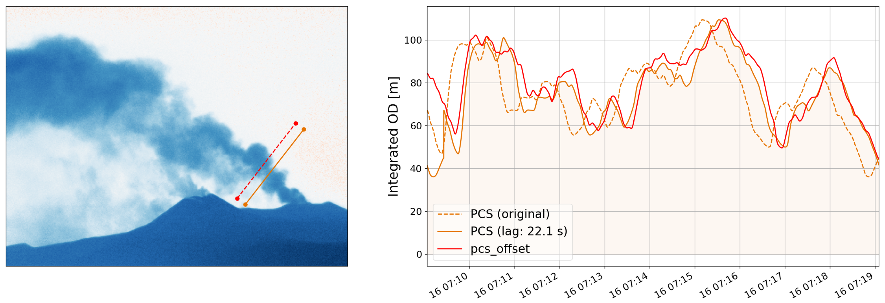
- Klein, A.; Lübcke, P.; Bobrowski, N.; Kuhn, J.; Platt, U. Plume propagation direction determination with SO2 cameras. Atmos. Meas. Tech. 2017, 10, 979–987. [Google Scholar] [CrossRef]
- Kern, C.; Deutschmann, T.; Vogel, L.; Wöhrbach, M.; Wagner, T.; Platt, U. Radiative transfer corrections for accurate spectroscopic measurements of volcanic gas emissions. Bull. Volcanol. 2010, 72, 233–247. [Google Scholar] [CrossRef]
- Kern, C.; Deutschmann, T.; Werner, C.; Sutton, A.J.; Elias, T.; Kelly, P.J. Improving the accuracy of SO2 column densities and emission rates obtained from upward-looking UV-spectroscopic measurements of volcanic plumes by taking realistic radiative transfer into account. J. Geophys. Res. Atmos. 2012, 117. [Google Scholar] [CrossRef]
- Vogel, L.; Galle, B.; Kern, C.; Delgado Granados, H.; Conde, V.; Norman, P.; Arellano, S.; Landgren, O.; Lübcke, P.; Alvarez Nieves, J.M.; et al. Early in-flight detection of SO2 via Differential Optical Absorption Spectroscopy: A feasible aviation safety measure to prevent potential encounters with volcanic plumes. Atmos. Meas. Tech. 2011, 4, 1785–1804. [Google Scholar] [CrossRef] [Green Version]
- Gliß, J. Geonum. 2016. Available online: https://github.com/jgliss/geonum (accessed on 11 September 2017).
- Farr, T.G.; Rosen, P.A.; Caro, E.; Crippen, R.; Duren, R.; Hensley, S.; Kobrick, M.; Paller, M.; Rodriguez, E.; Roth, L.; et al. The Shuttle Radar Topography Mission. Rev. Geophys. 2007, 45. [Google Scholar] [CrossRef]
- Amante, C.; Eakins, B.W. ETOPO1 Global Relief Model converted to PanMap layer format. NOAA-Natl. Geophys. Data Center PANGAEA 2009. [Google Scholar] [CrossRef]
- Kraus, S. DOASIS: A framework design for DOAS. Ph.D. Thesis, Universitat Mannheim, Mannheim, Germany, 2006. [Google Scholar]
- Farnebäck, G. Two-Frame Motion Estimation Based on Polynomial Expansion. In Proceedings of the 13th Scandinavian Conference on Image Analysis, (SCIA 2003), Halmstad, Sweden, 29 June–2 July 2003; Springer: Berlin, Germany, 2003; pp. 363–370. [Google Scholar]
- Bradski, G. The OpenCV Library. Dr. Dobb’s J. Softw. Tools 2000, 25, 120–123. [Google Scholar]
- Gliß, J.; Stebel, K.; Kylling, A.; Sudbø, A. Optical flow gas velocity analysis in plumes using UV cameras—Implications for SO2-emission rate retrievals investigated at Mt. Etna, Italy, and Guallatiri, Chile. Atmos. Meas. Tech. Discuss. 2017, 2017, 1–30. [Google Scholar] [CrossRef]
- Fong, D.C.L.; Saunders, M. LSMR: An Iterative Algorithm for Sparse Least-Squares Problems. SIAM J. Sci. Comput. 2011, 33, 2950–2971. [Google Scholar] [CrossRef]
Sample Availability: The Pyplis software is freely available, including the example data and scripts. For more information see http://pyplis.readthedocs.io. |


| Analysis Block | Quantities | Analysis Options | Section |
|---|---|---|---|
| Geometrical Calculations | 3.1 | ||
| Plume Background Analysis | , , | 3.3 | |
| Camera Calibration | Cell, DOAS | 3.4 | |
| Plume Velocity Retrieval | Optical flow, cross-correlation | 3.5 | |
| Emission rate | Signal dilution correction | 3.6, 3.7 |
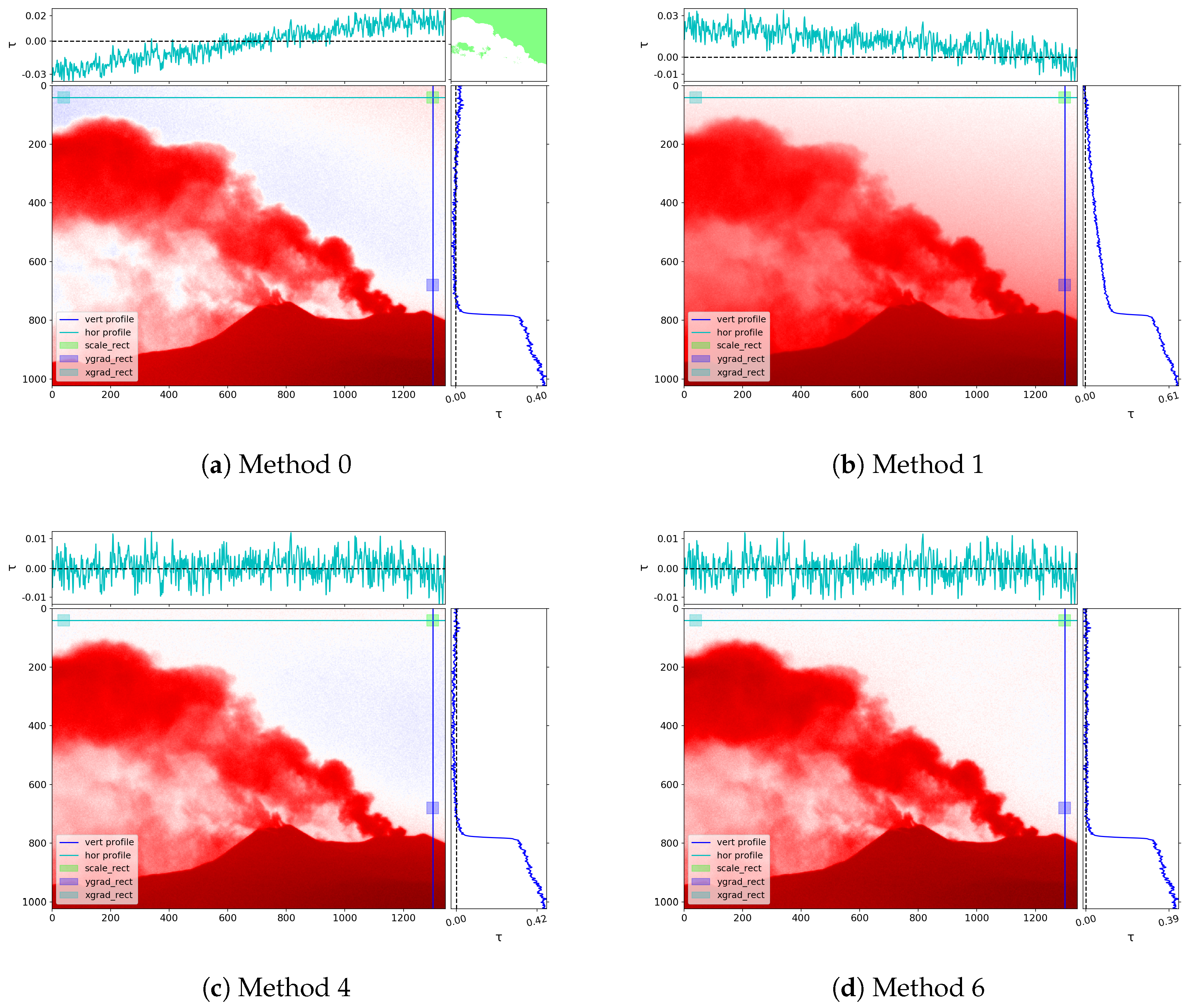
| Method | -img | Corrections | ||
|---|---|---|---|---|
| Scaling | Vertical | Horizontal | ||
| 1 | yes | Scaling in scale_rect | None | None |
| 2 | yes | See 1 | Linear correction using scale_rect and ygrad_rect | None |
| 3 | yes | See 1 | Curvature correction by fitting polynomial of n-th order using sky reference pixels along vertical profile line (default: n = 2, i.e., quadratic polynomial) | None |
| 4 | yes | See 1 | Linear correction (see 2) | Linear correction using scale_rect and xgrad_rect |
| 5 | yes | See 1 | Curvature correction (see 3) | Linear correction (see 4) |
| 6 | yes | See 1 | Curvature correction (see 3) | Curvature correction by fitting polynomial of n-th order using sky reference pixels along horizontal profile line (default: n = 2, i.e., quadratic polynomial) |
| 0 | no | Masked 2D polynomial surface fit | ||
| 99 | yes | None (use -img as is) | ||
© 2017 by the authors. Licensee MDPI, Basel, Switzerland. This article is an open access article distributed under the terms and conditions of the Creative Commons Attribution (CC BY) license (http://creativecommons.org/licenses/by/4.0/).
Share and Cite
Gliß, J.; Stebel, K.; Kylling, A.; Dinger, A.S.; Sihler, H.; Sudbø, A. Pyplis–A Python Software Toolbox for the Analysis of SO2 Camera Images for Emission Rate Retrievals from Point Sources. Geosciences 2017, 7, 134. https://doi.org/10.3390/geosciences7040134
Gliß J, Stebel K, Kylling A, Dinger AS, Sihler H, Sudbø A. Pyplis–A Python Software Toolbox for the Analysis of SO2 Camera Images for Emission Rate Retrievals from Point Sources. Geosciences. 2017; 7(4):134. https://doi.org/10.3390/geosciences7040134
Chicago/Turabian StyleGliß, Jonas, Kerstin Stebel, Arve Kylling, Anna Solvejg Dinger, Holger Sihler, and Aasmund Sudbø. 2017. "Pyplis–A Python Software Toolbox for the Analysis of SO2 Camera Images for Emission Rate Retrievals from Point Sources" Geosciences 7, no. 4: 134. https://doi.org/10.3390/geosciences7040134