
Developing a Cloud-Reduced MODIS Surface Reflectance Product for Snow Cover Mapping in Mountainous Regions

Department of Civil Engineering, K.N. Toosi University of Technology, Tehran 1996715433, Iran
*
Author to whom correspondence should be addressed.
Geosciences 2017, 7(2), 29; https://doi.org/10.3390/geosciences7020029
Submission received: 22 February 2017
/
Revised: 6 April 2017
/
Accepted: 12 April 2017
/
Published: 17 April 2017
(This article belongs to the Special Issue Cryosphere)
Abstract
:Cloud obscuration is a major problem for using Moderate Resolution Imaging Spectroradiometer (MODIS) images in different applications. This issue poses serious difficulties in monitoring the snow cover in mountainous regions due to high cloudiness in such areas. To overcome this, different cloud removal methods have been developed in the past where most of them use MODIS snow cover products and spatiotemporal dependencies of snow to estimate the undercloud coverage. In this study, a new approach is adopted that uses surface reflectance data in the cloud-free pixels and estimates the surface reflectance of a cloudy pixel as if there were no cloud. This estimation is obtained by subsequently applying the k-nearest neighbor and dynamic time compositing methods. The modified surface reflectance data are then utilized as inputs of a Normalized Difference Snow Index (NDSI)-based algorithm to map snow cover in the study area. The results indicate that the suggested approach is able to appropriately estimate undercloud surface reflectance in bands 2, 4 and 6, and can map the snow cover with 97% accuracy, which is a substantial improvement over the conventional method with an accuracy of 86%. Finally, although a clear underestimation of snow cover (about 15%) is observed by applying the proposed approach, still, it is much better than the 30% underestimation obtained by the conventional method.
1. Introduction
Snow is an important component of hydrological cycle. Accumulation in cold season and melt in warm season provide a large portion of water resources in different regions around the world. Thus, many efforts have been made to measure and accurately estimate it in river basins for better management of water resources. In situ measurements are the most common way to quantify snow variations. Such measurements are costly and limited to a few points that are mostly located in lower elevations of basins. However, snow varies drastically in temporal and spatial extent and it is mainly concentrated at higher elevations. In recent decades, the development of remote sensing technology has offered an alternative for snow monitoring. This technology provides near global coverage, high temporal and spatial resolution, and is able to measure different parameters.
Among others, the Moderate Resolution Imaging Spectroradiometer (MODIS) images are widely used for snow cover monitoring in recent years. Fine 500 m resolution, daily revisit time, well scientific developer team, and ease of access have made MODIS images a popular dataset for hydrological modeling [1,2,3,4] and climatologic studies [5,6,7,8,9]. However, the obscuration of earth surface by clouds in visible and near-infrared wavelengths causes a major challenge in snow cover mapping through MODIS images [10,11,12,13]. Different methods have been proposed to overcome this problem [14,15,16,17]. Most of these studies have focused on MODIS snow cover products (SCPs) (NASA, Washington, DC, USA), namely MOD10A1 and MYD10A1. These products contain binary information indicating either the presence or absence of snow or cloud. Therefore, every pixel in an image would be classified as one of the categories including snow, land or cloud. The applied methods employ the spatiotemporal dependencies to reclassify the pixels that are assigned as cloud to snow or land. For example, Hall et al. [16] represented a methodology to replace cloud-covered pixels by most recent cloud-free observation. The results indicated a 96% increase in observable pixels. Spatial dependencies were applied by Parajka et al. [18], where they used relative position of cloudy pixels to regional snow-line elevation to reclassify them. The applied method was validated using climate stations with snow depth measurements. The results indicated that the proposed method could reduce cloud coverage by 50% without any considerable change in snow-mapping accuracy. Dong and Menzel [19] introduced a conditional probability interpolation method using in situ snow depth measurements to overcome cloud obscuration in southwestern Germany. The presented methodology showed an accuracy of 92% during snow season. Combination of different methods was investigated by several studies [14,15,20,21]. They applied a set of spatial, temporal and multi-sensor methods in a sequence-based algorithm to reduce cloud coverage. For example, Da Ronco and De Michele [14] combined five cloud removal methods subsequently including combination of Aqua and Terra SCPs, conservative temporal combination, regional snow-line method, eight-day backward temporal and seasonal filter. The results indicated that combination of methods could remove clouds efficiently with an accuracy of 95%. Considering seasonal variations in accuracy of different cloud removal methods [20], Dariane et al. [21] developed a cloud removal algorithm to combine different methods to reduce cloudiness along with maintaining the accuracy of snow mapping. Their algorithm was able to remove 94% of clouds and preserve the accuracy by 93%. All of these studies use MODIS SCPs as input dataset of cloud removal methods. In this study, we investigated an innovative approach to achieve a cloud-reduced snow cover map. This approach utilizes MODIS surface reflectance data and estimates cloud-covered pixels’ surface reflectance as it would have been measured at earth surface level and as if there were no clouds. It means that we changed the problem of estimating pixel coverage in cloudy condition (i.e., land or snow) to the estimation of earth surface reflectance when the pixel is cloud-covered. The estimated surface reflectance would be used as input of an algorithm to map snow cover in the study area. This new approach is implemented and compared to the conventional approach (i.e., using snow cover maps) that has been applied by the previous studies.
2. Study Area and Data Sets
2.1. Study Area
The developed methodology is applied for Central Alborz region (35.2°–36.8° N. latitude, 50.3°–53.3° E. longitude) in north of Iran (Figure 1). Central Alborz is the middle part of the Alborz Mountain Ranges that supplies water for a population of about 21 million in the region. It covers an area of about 26,800 km2 and its elevation ranges from 0 to 5604 m a.s.l.. The region is subdivided into two main slopes. The northern slope climate is humid due to movement of moist air from the Caspian Sea. The mean precipitation over this slope is about 700 mm per year. The southern slope is located on the leeward side of the Alborz Mountain Ranges. Its climate is semi-arid with mean precipitation of about 250 mm per year [22]. The vegetation cover in Central Alborz is not dense and is dominated by alpine meadows and consists mainly of herbaceous and xerophilous plants [23]. The study area consists of nine major river basins including Latian, Haraz, Taleghan, Lar, Mamloo, Karaj, Firoozkuh, Sehezar, and Chaloos, with several tributaries.
2.2. Remotely Sensed Data
MODIS sensor captures data in 36 bands from visible to thermal infrared. We utilized MODIS/Terra surface reflectance daily L2G (MOD09GA) product, which provides bands 1–7 surface reflectance data with daily revisit time and 500 m spatial resolution. This product is corrected for aerosols and atmospheric gases and is associated with data product state quality assurance scientific datasets that could be used to determine cloud state in every pixel [24]. This dataset is obtained from the MODIS cloud mask (MOD35_L2) product. To cover the study period from 1 October 2002 to 31 September 2015, 4748 of h22v05 tiles of MOD09GA version 6 are acquired through the Reverb website [25] and are preprocessed. In this study, bands 2, 4 and 6 would be used in snow cover mapping algorithm and cloud state dataset would be utilized to determine cloud condition as cloud flag.
3. Methodology
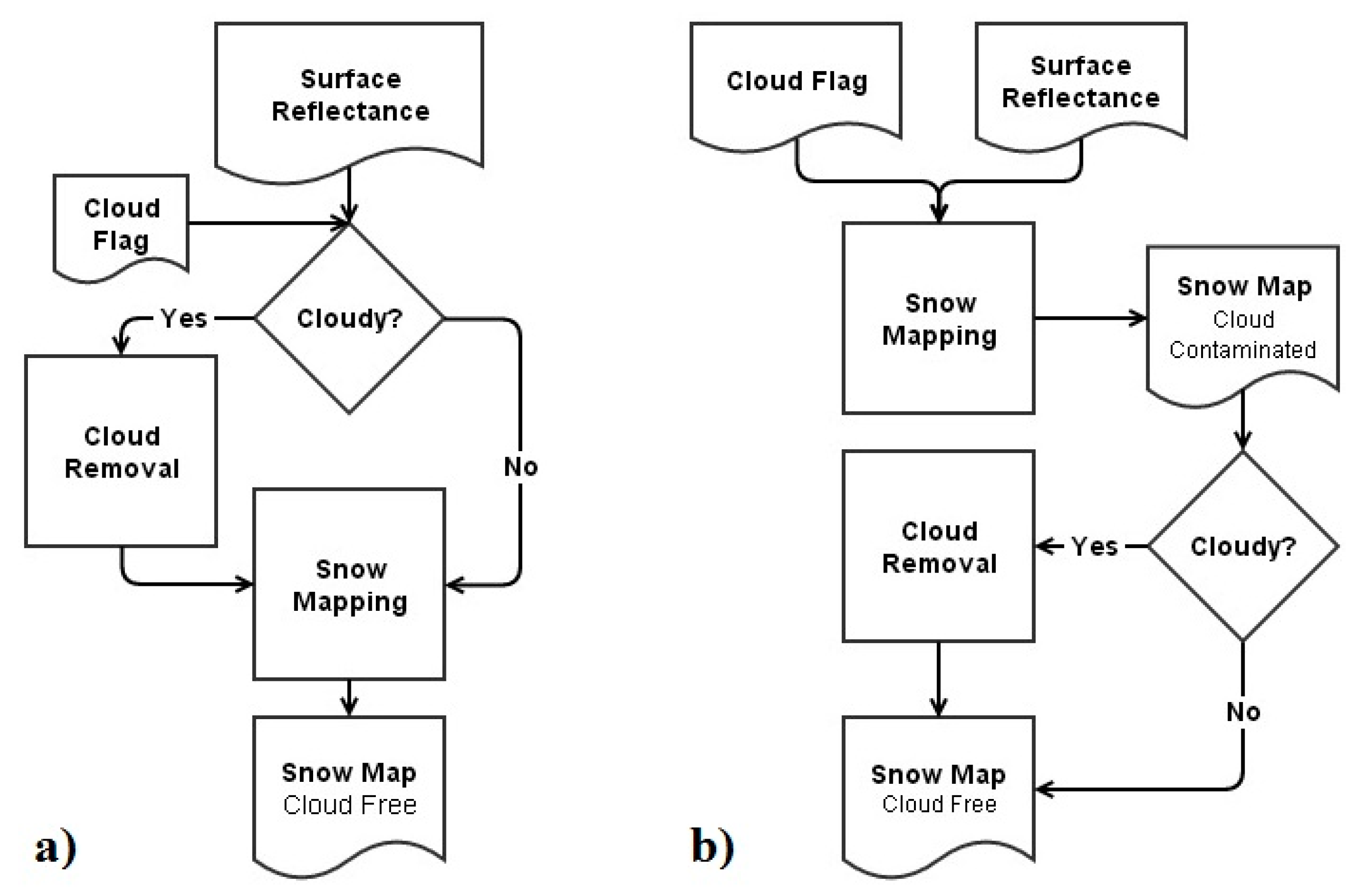
The adopted methodology estimates undercloud surface reflectance using a sequence-based combination of k-nearest neighbor method and dynamic time compositing. Then, estimated values would be used in snow cover detection algorithm to map snow cover in the study area. To identify the superiority of the proposed approach over the conventional method, a cloud removal algorithm using the same methods but with priority to snow mapping is implemented in parallel. The conventional approach uses cloud-contaminated surface reflectance data to map the snow cover and clouds. Then, it applies a cloud removal procedure to detect the surface coverage under the cloud. A scheme of both algorithms is given in Figure 2. To validate both algorithms, a validation methodology is adopted that fills cloud-free images with factitious clouds and assumes cloud-free images as the ground-truth for cloud-filled images. Detailed descriptions are presented in the sections that follow.
3.1. Cloud Removal Methods
3.1.1. K-Nearest Neighbors
This method uses eight neighbor pixels to estimate surface reflectance in a cloud-covered pixel. The estimation is obtained using the following equations:
where SF(x, y) is the target function and is equal to surface reflectance of a pixel in x-th column and y-th row, w(x′, y′) is the weighting function that returns the weight of every neighbor pixel at x′-th column and y′-th row based on its Euclidean distance. Cloudflag is the cloud state function that is equal to 1 and 0 for cloud and non-cloud conditions, respectively. In conventional approach, the target is estimating undercloud coverage (snow or land) and is obtained by assigning the most common coverage among eight neighbor pixels to the cloudy pixel. It means that if most of the neighbor pixels are classified as snow, the cloudy pixel would be classified as snow and vice versa. In the event that the number of cloudy and snow-covered pixels is equal, no decision would be made.
3.1.2. Dynamic Time Composite
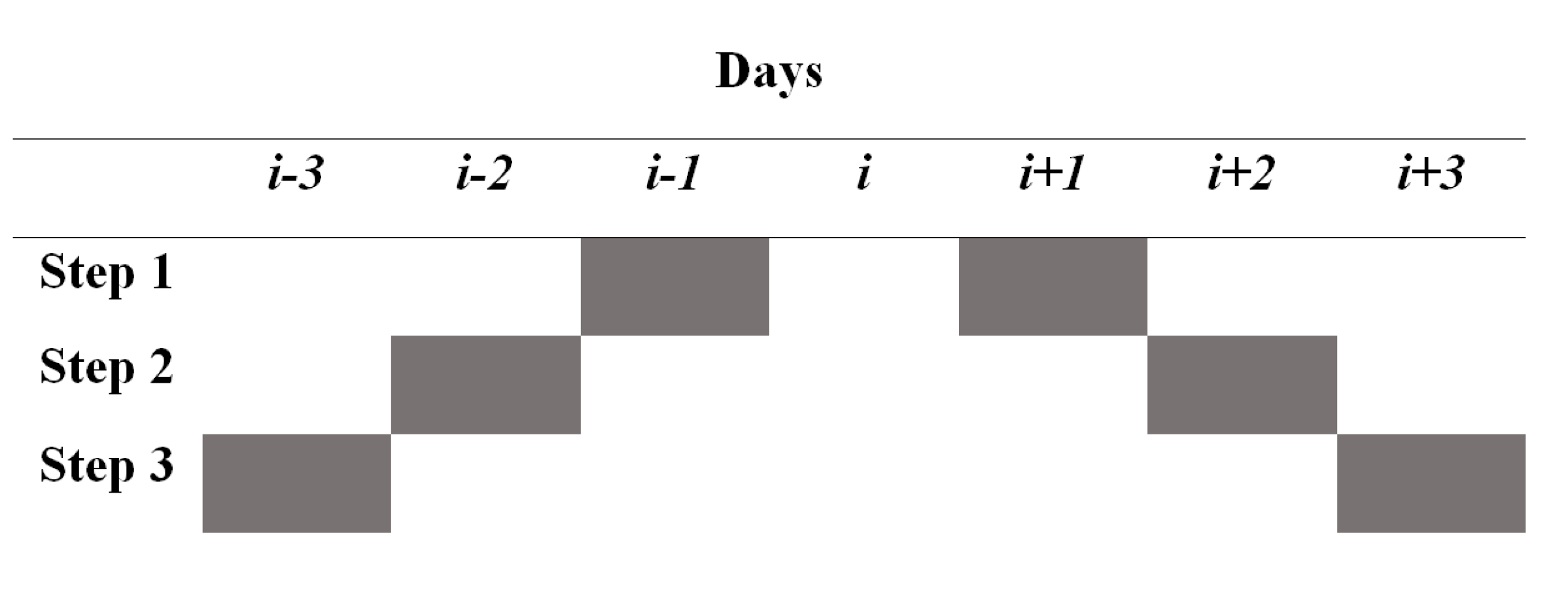
This method employs images of prior and subsequent days to estimate undercloud surface reflectance in a cloudy pixel. The time window that would be employed is two, four and six days. At the first step, this method tries to estimate surface reflectance using images of the preceding and following days. If the corresponding pixels were cloudy on both days, the method would use images of two days before and two days after. Finally, if these images were also cloud-covered, then images of three days before and after would be utilized. The employed days in each step are shown in Figure 3. The estimated undercloud surface reflectance would be equal to the (average) observed surface reflectance of non-cloudy day(s).
In conventional approach, the same steps would be used, but instead of surface reflectance values, the undercloud observation (snow or land) of the preceding or following days would be assigned to the cloudy pixel. In case of inconsistency, no action would be taken for the cloudy day.
3.1.3. Combination of Methods
The two above-described methods are combined in a sequence-based scheme. In this way, the k-nearest neighbor method is applied at first. This method is useful for the marginal pixels of clouds and/or cases with sparse small clouds. In the situation of large cloud areas, this method cannot work well. In such cases, the dynamic time composite method would be suitable and can remove the remaining parts of clouds. After applying each method, if the cloudiness is higher than a predetermined desired value (here 1%) the next method is applied. Figure 4 shows the flowchart of methods combination shows the flowchart of methods combination.
3.2. Snow Mapping
The applied snow-mapping algorithm is based on the Normalized Difference Snow Index (NDSI). This index is the normalized difference of band 4 (visible) and band 6 (shortwave infrared) in MODIS onboard Terra satellite. A pixel is classified as snow if the three following conditions are met [26].
- NDSI = > 0.4
- Band 2 reflectance > 11%
- Band 4 reflectance > 10%
Figure 5 shows the flowchart of the applied snow-mapping algorithm.
3.3. Validation Methodology
Due to the absence of in situ measurements, we used a validation methodology presented by Gafurov and Bardossy [15] and improved by Dariane et al. [21]. This method is based on assuming selected images with lowest cloudiness as ground truth and filling them with a cloud mask that is borrowed from among highly clouded images. Then, by applying cloud removal methods on cloud-filled images and comparing the resulted images with the corresponding ground truths (images with least cloud), the accuracy of cloud removal procedure is assessed. Hence, the validation results would show the agreement between low cloud images and cloud-removed ones. Therefore, in this study, the accuracy term is equal to agreement between these images in this study.
Using this methodology, 156 images (one image in every month during 13 years of study period) are selected as clear-sky images and filled with low, medium and high cloud masks. Cloud masks are picked out based on 25%, 50% and 75% probability of occurrences [21].
The results are validated in two forms. In the first, estimated surface reflectance values are validated using three criteria, including Root of Mean Square Error (RMSE), Mean Bias (MB), Coefficient of Determination (R2) and Pearson’s Correlation Coefficient (r). In the second form, snow-mapping accuracy is investigated. In this form, agreement between reclassified pixels and their corresponding pixels in ground truth images is assessed and is reported via a confusion matrix. This matrix shows the number of pixels that are correctly classified as snow (snow to snow), pixels that are misclassified as snow (land to snow), pixels that are correctly classified as land (land to land) and pixels that misclassified as land (snow to land). The total degree of agreement could be obtained as the rate of correctly classified pixels (snow to snow and land to land) to all the reclassified pixels.
4 Results
4.1. Cloud Removal Performance
The performance of a cloud removal method was assessed by the amount of clouds that could be removed applying the presented methodology. Figure 6 shows the time series of cloud coverage before and after cloud removal. In addition, monthly average cloud coverage during the study period is given in Table 1.
As can be seen from Table 1, the cloud removal substantially reduces the cloud contamination and removes about 94% of clouds during the study period. It is worthwhile to mention that both approaches would perform similarly in reducing the cloud coverage. In fact, they are essentially similar in this step although having different target functions, i.e., a continuous function in the presented approach and a discrete function in conventional approach. The main difference between the two approaches is on detecting the nature of area under the cloudy pixels.
4.2. Undercloud Surface Reflectance Estimation
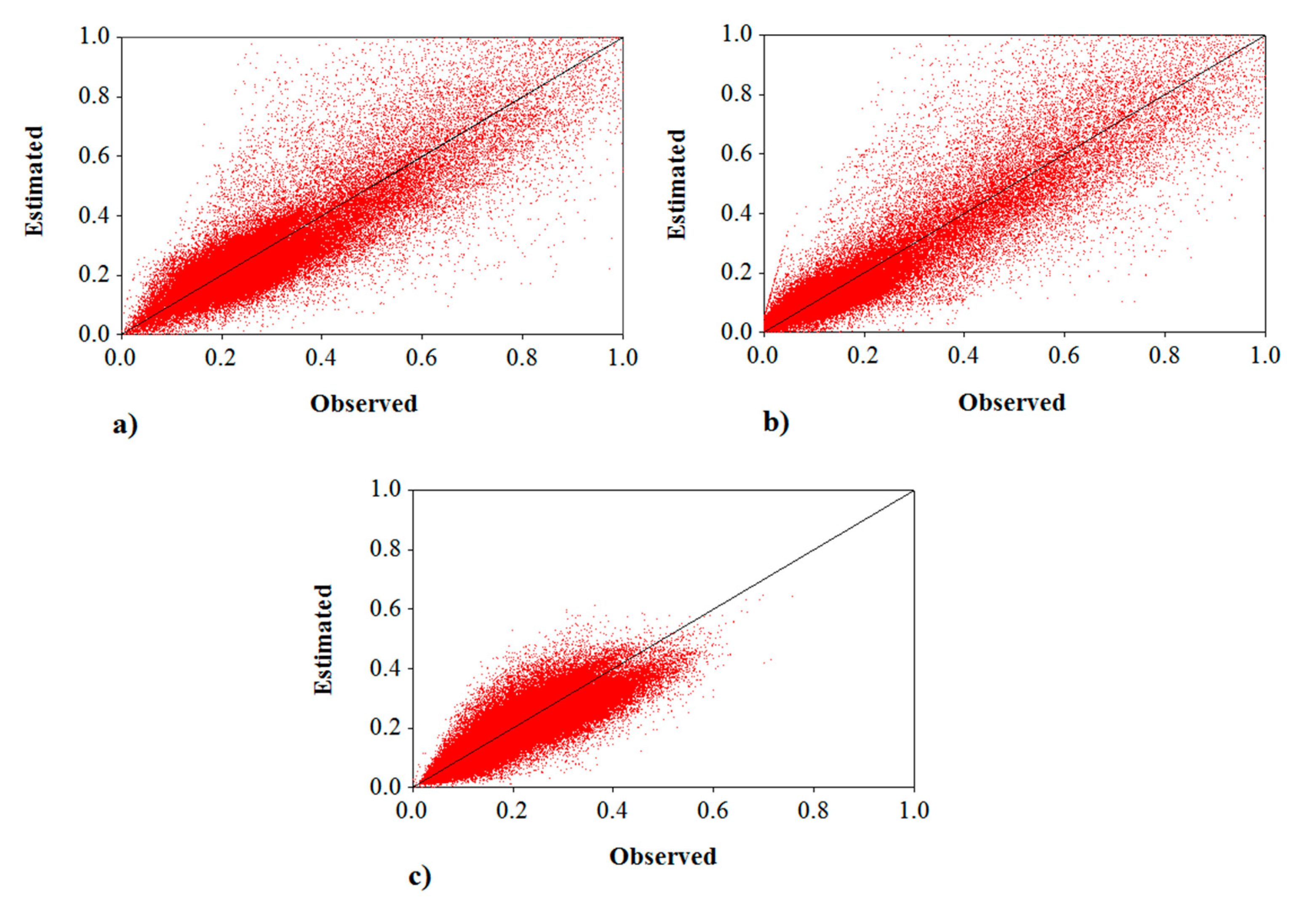
Undercloud surface reflectance was estimated in bands 2, 4 and 6 following the proposed approach. These bands were used in snow detection algorithm. In overall, surface reflectance of 112,737 pixels were reconstructed. Observed and estimated surface reflectance values are plotted against each other as shown in Figure 6. As can be seen from Table 2 as well as Figure 7, the proposed algorithm works well in bands 2 and 4; however, the accuracy of band 6 is not as good as the other two. The MB and RMSE are both under 0.1 in this band.
NDSI discriminates snow cover based on a threshold that is equal to 0.4. As long as the status of detected pixels is not changed, there is no snow-mapping error. It seems unlike the higher band 6 estimating error, the NDSI error does not effectively alter the precision of snow mapping by the proposed method.
4.3. Snow Mapping
As illustrated in Section 3.3, snow-mapping accuracy was investigated as the number of correctly classified and misclassified pixels in a confusion matrix form. Table 3 and Table 4 are the validation results for the two applied approaches. As is indicated in Table 3, 85.3% and 100% of snow and land reclassified pixels agree with original non-clouded snow cover map using the proposed approach, whereas, by applying the conventional approach, 70.2% and 91.4% of snow and land pixels are correctly reclassified (Table 4).
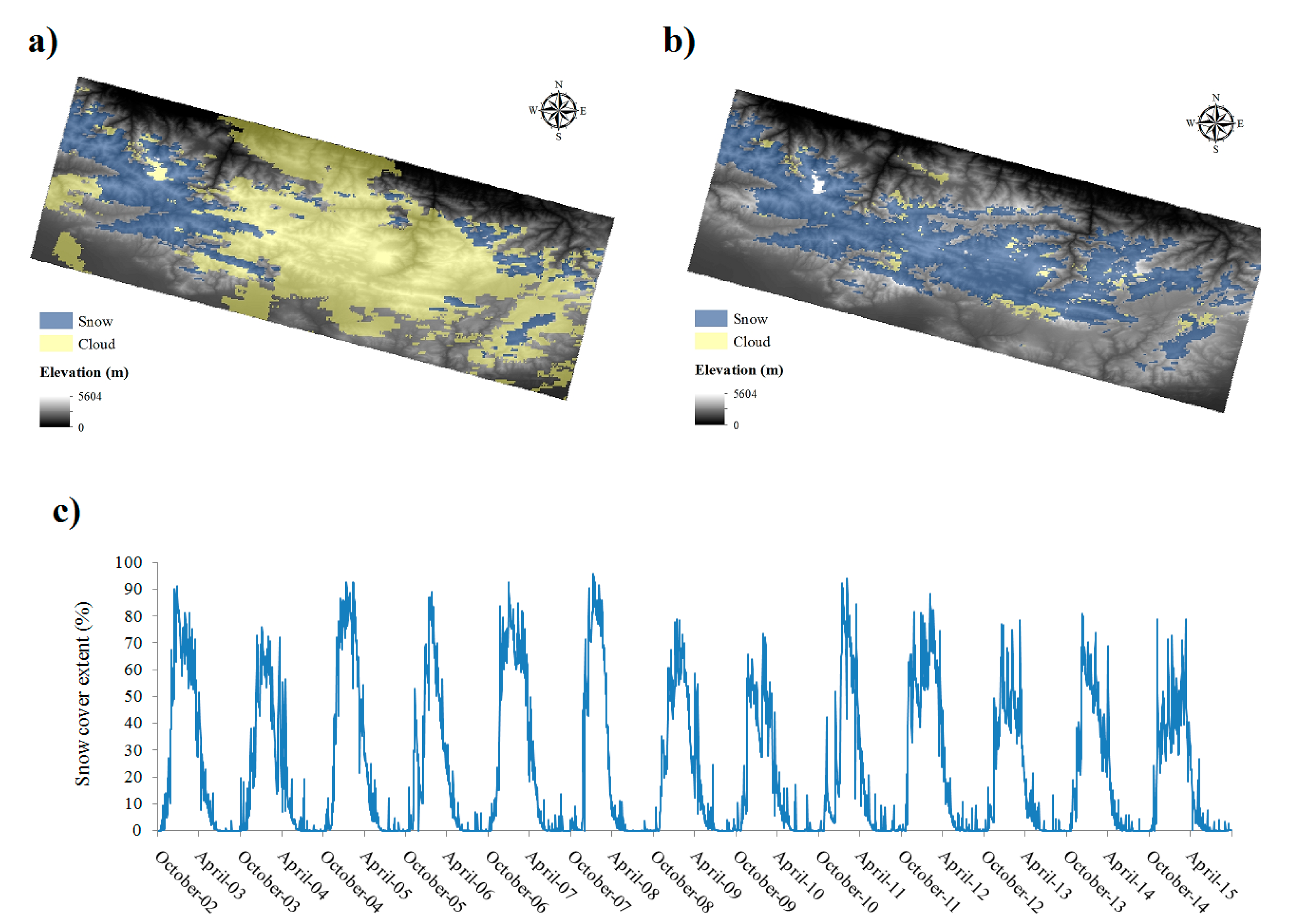
The overall accuracy of the proposed and conventional approaches is 97% and 86% in the study area, respectively. These results show that the proposed approach can reasonably improve the cloud removal accuracy in comparison to the conventional approach. Although a clear underestimation of snow cover (about 15%) can be found by applying the proposed approach, still, it is much better than the 30% underestimation obtained by the conventional method. A sample of obtained snow maps using the presented approach is given in Figure 8. This figure shows snow and cloud coverage before and after cloud removal at 1 February 2015. Also, variation of snow cover extent over the study region is estimated using cloud-removed snow maps (Figure 8c).
5. Discussion and Conclusions
Cloud obscuration is a major challenge in using MODIS images for snow cover mapping. Several studies have addressed this issue and have developed different methods to overcome this problem. Using spatiotemporal dependencies between MODIS snow cover binary maps is the cornerstone of all the past studies. In this work, we presented a new approach to reach a cloud-reduced snow cover map. The proposed approach estimates undercloud surface reflectance in the cloudy condition and uses estimated surface reflectance to map snow cover by applying a snow detection algorithm. This approach was compared to the conventional approach that, in the first step, maps the snow cover and labels the cloud-contaminated pixels as cloudy, and then approximates the undercloud area condition. The proposed approach utilized two sequential methods including k-nearest neighbor and dynamic time composite to estimate undercloud surface reflectance values.
Although the in situ measurements have to be used as ground-truth data, due to the absence of such measurements, an alternative methodology was followed. According to this approach, cloud-free images are assumed as ground truth data. Hence, the accuracy assessment results showed the agreement between cloud-removed images and cloud-free ones. Thus, cloud-removed snow cover maps would be with some uncertainties that are reported in previous studies [19,27].
Validation was done in two ways. In the first one, the estimated surface reflectance values in bands 2, 4 and 6 were validated. The results showed that the proposed approach is able to estimate the surface reflectance values with high precision. In the second way, mapped snow cover was compared with ground-truth images. The comparison indicated that snow condition could be classified correctly with the accuracy of 97% and 86% using the proposed approach and the conventional method, respectively, which indicates the superiority of the proposed approach. Finally, although a clear underestimation of snow cover (about 15%) was found by applying the proposed approach, still, it is much better than the 30% underestimation obtained by the conventional method. The superiority of the presented approach in the validation results could be due to better performance of cloud removal methods in approximating surface reflectance values (presented approach) in comparison to estimating binary snow cover conditions (conventional approach). In other words, approximating a real value could cause less error than a binary value potentially. In a binary system, only two values (0 or 1) can be selected, but in real numbers system, a continuous set of values are feasible. Therefore, a slight induction bias may produce less error in an obtained snow map using the presented approach. This reason is subjective and needs to be investigated more precisely in future studies.
The presented methodology is applicable in other snow-covered mountainous regions all over the world. However, the performance of method in terms of cloud reduction and the accuracy depends on the persistency of clouds and heterogeneity of land coverage. More continuous cloud persistency in the region demands an increased number of needed pervious and following day’s images. Under this situation, the uncertainty with estimated snow condition would increase. Also, the heterogeneity of land surface would pose the k-nearest neighbor method with difficulties in accurate estimation of undercloud condition.
Author Contributions
This research article is part of the Ph.D. level dissertation of the co-author, Amin Khoramian, under the supervision of the corresponding author, Alireza B. Dariane.
Conflicts of Interest
The authors declare no conflict of interest.
References
- Franz, K.J.; Karsten, L.R. Calibration of a distributed snow model using MODIS snow covered area data. J. Hydrol. 2013, 494, 160–175. [Google Scholar] [CrossRef]
- Parajka, J.; Blöschl, G. The value of MODIS snow cover data in validating and calibrating conceptual hydrologic models. J. Hydrol. 2008, 358, 240–258. [Google Scholar] [CrossRef]
- Berezowski, T.; Chormański, J.; Batelaan, O. Skill of remote sensing snow products for distributed runoff prediction. J. Hydrol. 2015, 524, 718–732. [Google Scholar] [CrossRef]
- Mcguire, M.; Wood, A.W.; Hamlet, A.F.; Lettenmaier, D.P. Use of satellite data for streamflow and reservoir storage forecasts in the Snake River Basin. J. Water Resour. Plan. Manag. 2006, 132, 97–110. [Google Scholar] [CrossRef]
- Wang, R.; Yao, Z.; Liu, Z.; Wu, S.; Jiang, L.; Wang, L. Snow cover variability and snowmelt in a high-altitude ungauged catchment. Hydrol. Process. 2015, 29, 3665–3676. [Google Scholar] [CrossRef]
- Tang, Z.; Wang, J.; Li, H.; Yan, L. Spatiotemporal changes of snow cover over the Tibetan plateau based on cloud-removed moderate resolution imaging spectroradiometer fractional snow cover product from 2001 to 2011. J. Appl. Remote Sens. 2013, 7, 73582. [Google Scholar] [CrossRef]
- Tahir, A.A.; Chevallier, P.; Arnaud, Y.; Ashraf, M.; Bhatti, M.T. Snow cover trend and hydrological characteristics of the Astore River basin (Western Himalayas) and its comparison to the Hunza basin (Karakoram region). Sci. Total Environ. 2014, 505, 748–761. [Google Scholar] [CrossRef] [PubMed]
- She, J.; Zhang, Y.; Li, X.; Feng, X. Spatial and temporal characteristics of snow cover in the Tizinafu watershed of the Western Kunlun Mountains. Remote Sens. 2015, 7, 3426–3445. [Google Scholar] [CrossRef]
- Paudel, K.P.; Andersen, P. Monitoring snow cover variability in an agropastoral area in the Trans Himalayan region of Nepal using MODIS data with improved cloud removal methodology. Remote Sens. Environ. 2011, 115, 1234–1246. [Google Scholar] [CrossRef]
- Parajka, J.; Blöschl, G. Validation of MODIS snow cover images over Austria. Hydrol. Earth Syst. Sci. 2006, 10, 679–689. [Google Scholar] [CrossRef]
- Andreadis, K.M.; Lettenmaier, D.P. Assimilating remotely sensed snow observations into a macroscale hydrology model. Adv. Water Resour. 2006, 29, 872–886. [Google Scholar] [CrossRef]
- Tekeli, A.E.; Akyürek, Z.; Arda Şorman, A.; Şensoy, A.; Ünal Şorman, A. Using MODIS snow cover maps in modeling snowmelt runoff process in the eastern part of Turkey. Remote Sens. Environ. 2005, 97, 216–230. [Google Scholar] [CrossRef]
- Wang, X.; Xie, H.; Liang, T.; Huang, X. Comparison and validation of MODIS standard and new combination of Terra and Aqua snow cover products in northern Xinjiang, China. Hydrol. Process. 2009, 23, 419–429. [Google Scholar] [CrossRef]
- Da Ronco, P.; De Michele, C. Cloud obstruction and snow cover in Alpine areas from MODIS products. Hydrol. Earth Syst. Sci. 2014, 18, 4579–4600. [Google Scholar] [CrossRef]
- Gafurov, A.; Bardossy, A. Cloud removal methodology from MODIS snow cover product. Hydrol. Earth Syst. Sci. 2009, 13, 1361–1373. [Google Scholar] [CrossRef]
- Hall, D.K.; Riggs, G.A.; Foster, J.L.; Kumar, S.V. Development and evaluation of a cloud-gap-filled MODIS daily snow-cover product. Remote Sens. Environ. 2010, 114, 496–503. [Google Scholar] [CrossRef]
- Wang, X.; Zheng, H.; Chen, Y.; Liu, H.; Liu, L.; Huang, H.; Liu, K. Mapping snow cover variations using a MODIS daily cloud-free snow cover product in northeast China. J. Appl. Remote Sens. 2014, 8, 084681. [Google Scholar] [CrossRef]
- Parajka, J.; Pepe, M.; Rampini, A.; Rossi, S.; Blöschl, G. A regional snow-line method for estimating snow cover from MODIS during cloud cover. J. Hydrol. 2010, 381, 203–212. [Google Scholar] [CrossRef]
- Dong, C.; Menzel, L. Producing cloud-free MODIS snow cover products with conditional probability interpolation and meteorological data. Remote Sens. Environ. 2016, 186, 439–451. [Google Scholar] [CrossRef]
- Parajka, J.; Blöschl, G. Spatio-temporal combination of MODIS images—Potential for snow cover mapping. Water Resour. Res. 2008, 44, W03406. [Google Scholar] [CrossRef]
- Dariane, A.B.; Khoramian, A.; Santi, E. Investigating Spatiotemporal Snow Cover Variability via Cloud-free MODIS Snow Cover Product in Central Alborz region. Remote Sens. Environ. 2017, in press. [Google Scholar]
- Islamic Republic of Iran Meteorological Organization (IRIMO). Annual Report of National Crisis Management and Climatic Hazards; IRIMO: Tehran, Iran, 2014. [Google Scholar]
- Mossadegh, A. Aperçu général sur les hêtraies montagnardes des forêts de la Caspienne en Iran. Rev. For. Fr. 1968, 20–27. Available online: http://documents.irevues.inist.fr/bitstream/handle/2042/24925/RFF_1968_1_20.pdf?sequence=1&isAllowed=y (accessed on 17 April 2017). [CrossRef]
- Vermote, E.F.; Kotchenova, S.Y.; Ray, J.P. MODIS Land Surface Reflectance Science Computing Facility. In MODIS Surface Reflectance User’s Guide; version 1.4; National Aeronautics and Space Administration (NASA): Washington, DC, USA, 2011. [Google Scholar]
- Reverb, The Next Generation Metadata and Service Discovery Tool. Available online: https://reverb.echo.nasa.gov/reverb (accessed on 15 September 2016).
- Hall, D.K.; Riggs, G.A.; Salomonson, V.V.; DiGirolamo, N.E.; Bayr, K.J. MODIS snow-cover products. Remote Sens. Environ. 2002, 83, 181–194. [Google Scholar] [CrossRef]
- Dong, C.; Menzel, L. Improving the accuracy of MODIS 8-day snow products with in situ temperature and precipitation data. J. Hydrol. 2016, 534, 466–477. [Google Scholar] [CrossRef]
Figure 1.
Study area.
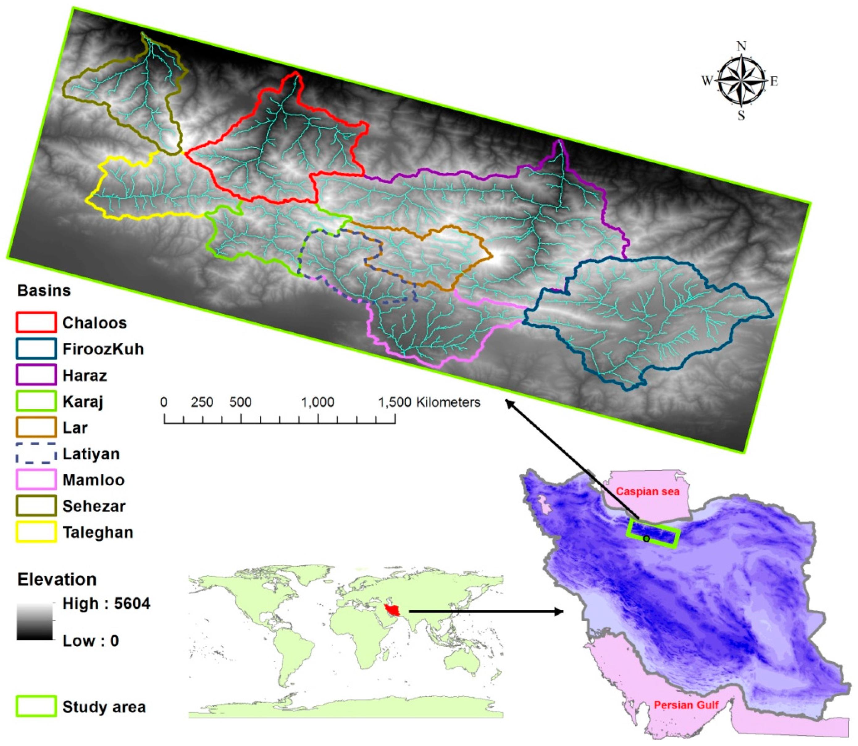
Figure 2.
Applied algorithms (a) Proposed approach; (b) Conventional approach.

Figure 3.
Utilized days in each step for dynamic time composite.

Figure 4.
Flowchart of methods combination.
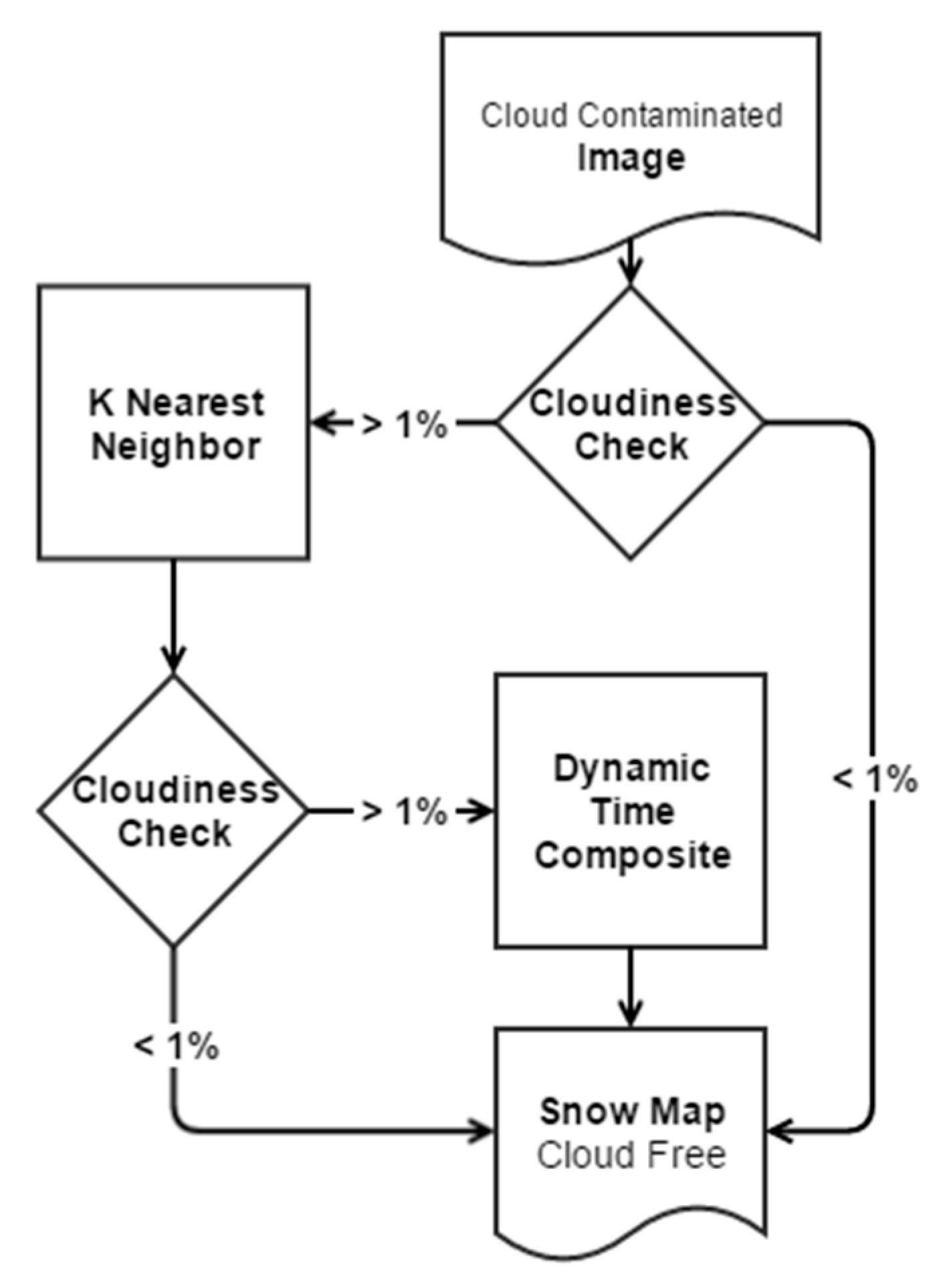
Figure 5.
Flowchart of applied snow-mapping algorithm.
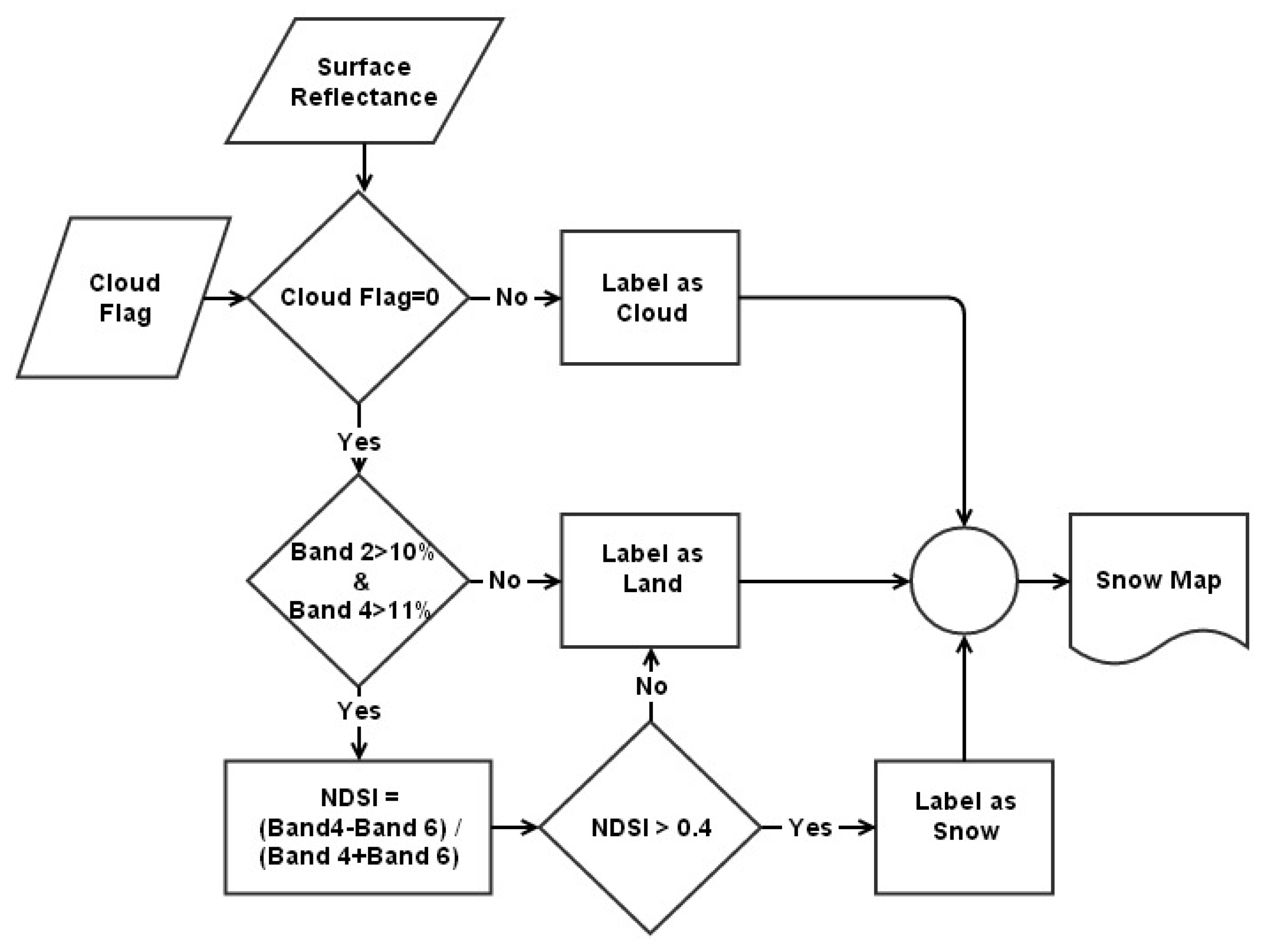
Figure 6.
Time series of cloud coverage before and after cloud removal.
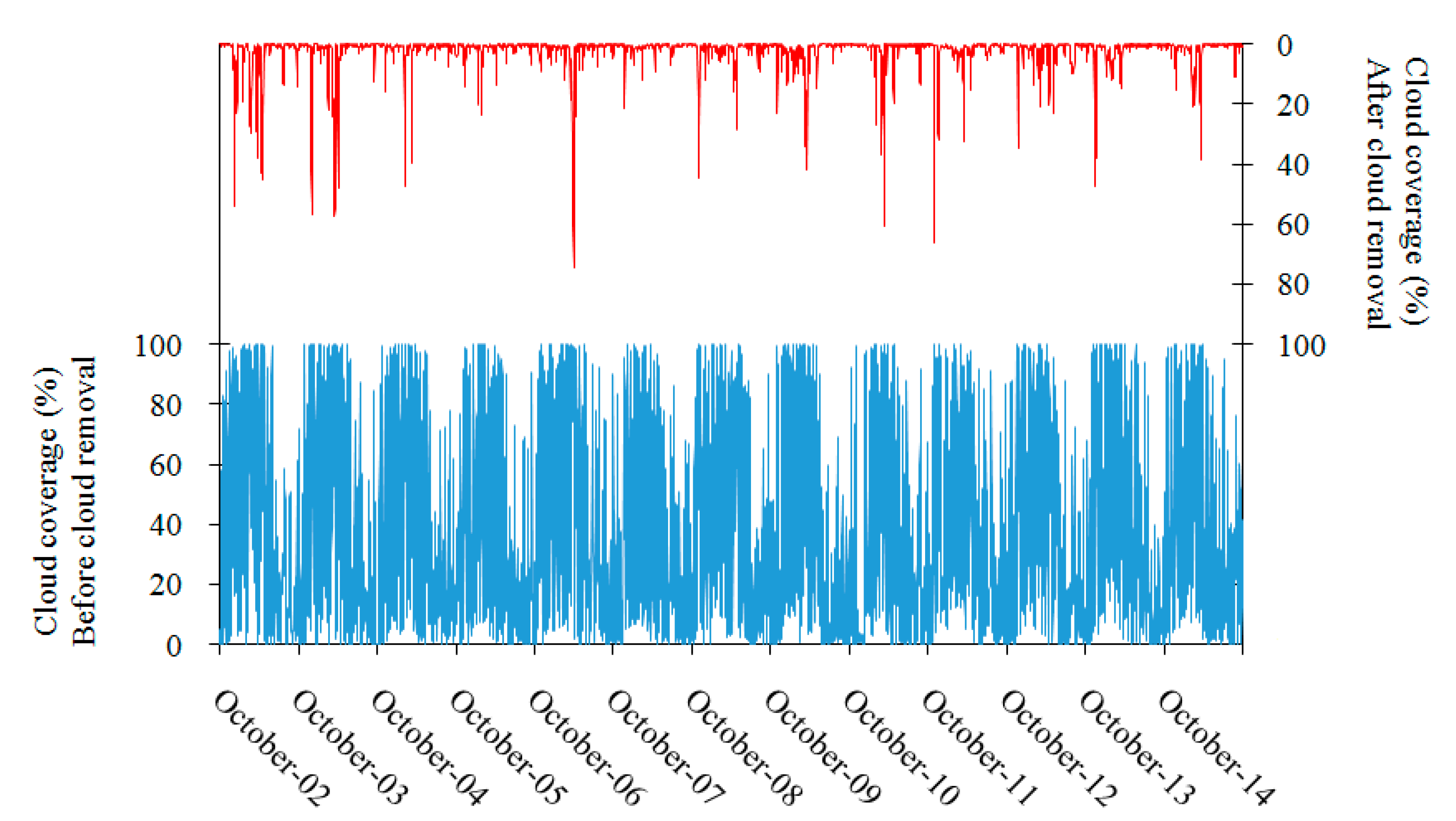
Figure 7.
Observed against estimated surface reflectance for (a) band 2, (b) band 4 and (c) band 6.

Figure 8.
Snow and cloud maps of study region (a) before and (b) after implementation of proposed cloud removal approach on 1 February 2015, and (c) time series of snow cover extent extracted from obtained snow maps during the study period (2002–2015).
Figure 8.
Snow and cloud maps of study region (a) before and (b) after implementation of proposed cloud removal approach on 1 February 2015, and (c) time series of snow cover extent extracted from obtained snow maps during the study period (2002–2015).


Table 1.
Average cloud coverage with and without cloud removal during the study period (2002–2015).
| Cloudiness | Winter | Autumn | Spring | Summer | Annual |
|---|---|---|---|---|---|
| Original amount of cloud (%) | 56.3 | 38.0 | 18.7 | 38.3 | 37.8 |
| Remained cloud (%) | 4.3 | 1.7 | 1.0 | 2.1 | 2.2 |
| Percent reduction | 92.3 | 95.6 | 94.9 | 94.6 | 94.1 |
Table 2.
Validation criteria for bands 2, 4 and 6. RMSE: Root of Mean Square Error.
| Validation Criteria | Band 2 | Band 4 | Band 6 |
|---|---|---|---|
| Mean Bias | 0.066 | 0.054 | 0.051 |
| RMSE | 0.09 | 0.082 | 0.063 |
| R2 | 0.75 | 0.85 | 0.61 |
| r | 0.87 | 0.92 | 0.85 |
Table 3.
Confusion matrix for the presented approach.
| Original Snow Map | Cloud-Removed Snow Map | ||
|---|---|---|---|
| Snow | Land | In Overall | |
| Snow | 22,146 (85.3%) | 3830 (14.7%) | 25,976 |
| Land | 0 (0%) | 86,761 (100%) | 86,761 |
| In overall | 22,146 | 90,591 | 112,737 |
| Overall accuracy: | 97% | ||
Table 4.
Confusion matrix for the conventional approach.
| Original Snow Map | Cloud-Removed Snow Map | ||
|---|---|---|---|
| Snow | Land | In Overall | |
| Snow | 18,224 (70.2%) | 7752 (29.8%) | 25,976 |
| Land | 7422 (8.6%) | 79,340 (91.4%) | 86,761 |
| In overall | 22,146 | 90,591 | 112,737 |
| Overall accuracy: | 86% | ||
© 2017 by the authors. Licensee MDPI, Basel, Switzerland. This article is an open access article distributed under the terms and conditions of the Creative Commons Attribution (CC BY) license (http://creativecommons.org/licenses/by/4.0/).
Share and Cite
MDPI and ACS Style
Khoramian, A.; Dariane, A.B. Developing a Cloud-Reduced MODIS Surface Reflectance Product for Snow Cover Mapping in Mountainous Regions. Geosciences 2017, 7, 29. https://doi.org/10.3390/geosciences7020029
AMA Style
Khoramian A, Dariane AB. Developing a Cloud-Reduced MODIS Surface Reflectance Product for Snow Cover Mapping in Mountainous Regions. Geosciences. 2017; 7(2):29. https://doi.org/10.3390/geosciences7020029
Chicago/Turabian StyleKhoramian, Amin, and Alireza B. Dariane. 2017. "Developing a Cloud-Reduced MODIS Surface Reflectance Product for Snow Cover Mapping in Mountainous Regions" Geosciences 7, no. 2: 29. https://doi.org/10.3390/geosciences7020029
Note that from the first issue of 2016, this journal uses article numbers instead of page numbers. See further details here.