Role of Faults in Hydrocarbon Leakage in the Hammerfest Basin, SW Barents Sea: Insights from Seismic Data and Numerical Modelling

1
Research Geoscientist at Shell Global Solutions International B.V., Kessler Park 1, 2288 GS Rijswijk, The Netherlands
2
Senior Geologist & Petroleum System Analyst at TOTAL Exploration & Production, La Défence 6, 2 Pl. Jean Millier, 92078 Paris, France
3
Petroleum System Analyst, Lundin Norway AS, Strandveien 4, N-1366 Lysaker, Norway
*
Author to whom correspondence should be addressed.
†
Research conducted in a former affiliation: GFZ German Research Centre for Geosciences, Telegrafenberg, 14473 Potsdam, Germany.
Geosciences 2017, 7(2), 28; https://doi.org/10.3390/geosciences7020028
Submission received: 29 January 2017
/
Revised: 27 March 2017
/
Accepted: 10 April 2017
/
Published: 15 April 2017
(This article belongs to the Special Issue Natural Gas Origin, Migration, Alteration and Seepage)
Abstract
:Hydrocarbon prospectivity in the Greater Barents Sea remains enigmatic as gas discoveries have dominated over oil in the past three decades. Numerous hydrocarbon-related fluid flow anomalies in the area indicate leakage and redistribution of petroleum in the subsurface. Many questions remain unanswered regarding the geological driving factors for leakage from the reservoirs and the response of deep petroleum reservoirs to the Cenozoic exhumation and the Pliocene-Pleistocene glaciations. Based on 2D and 3D seismic data interpretation, we constructed a basin-scale regional 3D petroleum systems model for the Hammerfest Basin (1 km × 1 km grid spacing). A higher resolution model (200 m × 200 m grid spacing) for the Snøhvit and Albatross fields was then nested in the regional model to further our understanding of the subsurface development over geological time. We tested the sensitivity of the modeled petroleum leakage by including and varying fault properties as a function of burial and erosion, namely fault capillary entry pressures and permeability during glacial cycles. In this study, we find that the greatest mass lost from the Jurassic reservoirs occurs during ice unloading, which accounts for a 60–80% reduction of initial accumulated mass in the reservoirs. Subsequent leakage events show a stepwise decrease of 7–25% of the remaining mass from the reservoirs. The latest episode of hydrocarbon leakage occurred following the Last Glacial Maximum (LGM) when differential loading of Quaternary strata resulted in reservoir tilt and spill. The first modeled hydrocarbon leakage event coincides with a major fluid venting episode at the time of a major Upper Regional angular Unconformity (URU, ~0.8 Ma), evidenced by an abundance of pockmarks at this stratigraphic interval. Our modelling results show that leakage along the faults bounding the reservoir is the dominant mechanism for hydrocarbon leakage and is in agreement with observed shallow gas leakage indicators of gas chimneys, pockmarks and fluid escape pipes. We propose a conceptual model where leaked thermogenic gases from the reservoir were also locked in gas hydrate deposits beneath the base of the glacier during glaciations of the Hammerfest Basin and decomposed rapidly during subsequent deglaciation, forming pockmarks and fluid escape pipes. This is the first study to our knowledge to integrate petroleum systems modelling with seismic mapping of hydrocarbon leakage indicators for a holistic numerical model of the subsurface geology, thus closing the gap between the seismic mapping of fluid flow events and the geological history of the area.
1. Introduction
The Greater Barents Sea has proven to be a challenging exploration frontier, but still contains much unlocked potential yet to be discovered, in particular with the opening of the formerly disputed area between Norway and Russia in 2013 [1,2,3,4,5,6].
Following the discoveries of large oil accumulations, namely the Johan Castberg (formerly Skrugard), Wisting and Gotha fields in 2011–2013 [6], exploration interest has rapidly risen in the Greater Barents Sea. However, these promising discoveries challenged previous theories of hydrocarbon prospectivity and occurrences, as most discoveries in the Barents Sea have been dominated by gas. In the last decade, the main exploration efforts focused on the Hammerfest Basin (Figure 1), in particular on the Snøhvit field [7,8,9,10], shown in Figure 1 and Figure 2. Multiple hydrocarbon leakage anomalies, paleo fluid contacts [11], under-filled structures and dominance of gas over oil demonstrate a complex history of fill-spill and leakage of hydrocarbons in the area [12,13,14,15,16,17]. Severe Cenozoic erosion and exhumation episodes during the Oligocene-Miocene [18,19], as well as the Pliocene-Pleistocene glaciations [12,20] are thought to have played a key role in the history of petroleum generation, migration, accumulation and leakage [10,19,20,21,22]. This was attributed to rapid overburden removal, change of spill points and trap geometry during glaciation, in-reservoir phase change and leakage of hydrocarbons from traps [19,21,23,24,25]. The last of these glaciations is marked by the Last Glacial Maximum (LGM), defined as the period 23,000–19,000 years before the present [26,27,28], when most of Northern Europe was covered by an extensive ice sheet, accompanied by reduced sea level and strong variations in Earth’s climate [28]. Nonetheless, to fully understand the processes controlling petroleum charge, migration and leakage, as well as petroleum phase prediction, a truly holistic approach is required, integrating seismic data interpretation, geochemistry and geological boundary conditions over time. This is typically achieved via 3D petroleum systems analysis and modelling (PSA and PSM). Recent 2D and coarse-resolution 3D petroleum system models in the Hammerfest Basin showed episodic leakage from Jurassic reservoirs, peaking during deglaciations [10,29], which agreed with the timing of seismically-observed hydrocarbon leakage indicators based on 2D and 3D seismic reflection datasets [16,30]. Past petroleum system modelling studies were coarse and first focused on the implementation of glacial cycles in 2D [10], followed by a 3D PSM study at a 2 km × 2 km scale grid resolution, where petroleum leakage was addressed explicitly by capillary leakage though seal failure. Moreover, recent studies of the Barents Sea revealed that the key regional faults (Figure 1 and Figure 3) in the Hammerfest Basin, namely NS, SW-NE and NW-SE faults [13,17], play a key role in petroleum migration from deeper Jurassic reservoirs (Figure 3 and Figure 4) to the shallow stratigraphy and up to the seabed [16,17,30], resulting in pockmarks (Figure 4 and Figure 5), inferred gas hydrates [30,31], amplitude anomalies, gas chimneys (Figure 3 and Figure 4) and shallow gas accumulations [16,30,32,33]. Evidence of condensate type light hydrocarbons charging the seabed sediments also indicate a deep origin of the fluids and present-day microseepage [34]. These compelling results revealed that the processes of hydrocarbon leakage and tertiary remigration in the Hammerfest Basin remains poorly understood due to geological uncertainties in the petroleum system models from the perspective of petroleum leakage. In this study, we integrate findings from 3D seismic data interpretation and analysis (Figure 3), detailed fault mapping, hydrocarbon leakage indicators (Figure 4 and Figure 5) coupled with improved granularity in a 3D petroleum system model to provide a higher resolution holistic Earth model. With this approach, we aim to reveal the impact of Pliocene-Pleistocene glaciations on hydrocarbon remigration and leakage from the Snøhvit and Albatross fields, which could serve as the analogue for de-risking of petroleum prospects in the Barents Sea. The results will also have implications for CO2 capture and storage efforts and associated risks at Snøhvit field [8,32].
2. Geological and Structural Setting
The geological evolution of the Barents Sea has been previously studied in detail by several authors [3,4,35,36,37,38]. The regional stratigraphy of the Barents Sea has also been discussed widely [39,40,41] with the formal nomenclature for the lithostratigraphy in the SW Barents Sea defined by [40,42].
In this communication, we focus on the stratigraphy, tectonic features and events including Triassic and younger (Figure 2 and Figure 3), with the focus on the following key sequences and boundaries: (1) present-day seabed, marked by numerous fluid escape features [15,16], (2) the Upper Regional Unconformity (URU) [43]: a diachronous angular unconformity marking the erosional base of multiple glacial episodes (0.8 Ma [16,20,44,45]); (3) a Cenomanian-Campanian polygonal fault interval [17]; and (4) the Bajocian Stø Formation, the main reservoir of the Snøhvit, Albatross and Askeladd fields [9,13].
The Hammerfest Basin (Figure 1) has an ENE-WSW axis trend, bounded by several regional fault complexes: the Troms-Finnmark Fault Complex, the Asterias Fault Complex and the Ringvassøy-Loppa Fault complex to the west, which separate the Hammerfest Basin (HB) from surrounding basins, highs and platforms [35]. The structural trends, the fault classes and their interactions in the Hammerfest Basin have been described in detail by [17]. The Hammerfest Basin is dominated by E-W trending faults (Figure 1 and Figure 2), as well as less abundant NS, SW-NE and NW-SE faults, repeatedly reactivated coeval with regional tectonic events [17,46]. The reactivated faults (Figure 3) are termed first order faults [17] and are found along older Triassic lineaments, which have been reactivated during recent Eocene tectonic events and penetrate through Cretaceous strata, Cenomanian polygonal fault tiers and into Paleocene-Early Eocene strata (Figure 3 and Figure 4). The Paleocene-Early Eocene strata are dissected by multiple curvilinear faults, termed PEEFs (Paleocene-Early Eocene Faults [17]), which are related to the preferential reactivation of polygonal faults [17]. The second order faults (Figure 3) are sealed below the Cenomanian, do not penetrate the Cenozoic successions [17] and are related to older transtensional events during the Kimmeridgian [46]. The Snøhvit field (Figure 1 and Figure 2) is situated in an EW trending horst, bounded by EW trending reactivated faults (Figure 3). The first order reactivated, as well as second order fault classes (Figure 3 and Figure 4), where first order has been reactivated in the Cenozoic (Paleocene-Early Eocene, Figure 2) and up to 0.8 Ma (age of URU [20,45,47]), whereas the second order faults have been reactivated during Albian and Cenomanian time [17].
The main reservoir is represented by the Middle Jurassic Stø Formation (Figure 2 and Figure 3), consisting of shallow marine lagoonal and estuarine barrier sands [9] with additional reservoirs in lower coastal plain shallow marine deposits of the Lower Jurassic Nordmela Formation and upper coastal plain fluvial deposits of the Lower Jurassic Tubæn Formation [7,9]. The anoxic Hekkingen Formation (Figure 2) shale is a proven source rock in the SW Barents Sea with high Total Organic Carbon contents (up to 20% TOC [13]), as well as a high Hydrogen Index (HI), with potential to generate dominantly liquid petroleum [7]. Other prominent source rocks include the Lower Jurassic shales and coals of the Nordmela Formation with potential to generate waxy oils and gas [13]. Additional source rocks in the SW Barents Sea include the Triassic shales (Figure 3), namely the Kobbe, Snadd and Fruholmen Formations, with mainly gas potential [7,29].
The sealing rocks for the Snøhvit and Albatross fields consist of the Upper Jurassic Fuglen and Hekkingen Formations (Figure 2 and Figure 3). The thicknesses of these formations are 7–30 m and 60–80 m, respectively [40]. The maturity of the Jurassic source rock sequences is variable (Figure 3): they are immature in the immediate vicinity of the Snøhvit and Albatross fields, within the oil window in the NW of the study area, where the Hammerfest Basin deepens, and in the gas window in Tromsø Basin, whereas the Triassic source rocks are mainly within the gas window [7,29].
Three main erosional periods have been reported in this area: Late Cretaceous, Eocene-Oligocene (35–40 Ma) and Miocene (5–10 Ma), with average erosional thicknesses of 200, 1000 and 500 m, respectively [7,18]. Additionally, a net overburden thickness of 500 m was removed during the Pliocene-Pleistocene through glacio-fluvial processes in the Hammerfest Basin, preferentially due to glacial ice streams [20]. The erosion boundary is marked by the Upper Regional Unconformity (URU, Figure 2 and Figure 3) [43].
3. Materials and Methods: Construction of the 3D Petroleum System Model
3.1. Input Data
Interpretation of ~32,000,000 km of 2D and 1000 km2 of 3D seismic data allowed us to build a 90 km × 60 km 3D subsurface Earth model, gridded at 0.5 km × 0.5 km spacing, with fourteen stratigraphic layers (~0.32 million cells), which includes an updated glacial history, as well as key regional and prospect-scale faults (Figure A1). The petroleum system model building, simulation and visualization were done using PetroMod® v. 2012 software (Schlumberger, Houston, TX, USA), which included nesting of a high resolution prospect-scale model within a larger regional-scale basin model, using Local Grid Refinement (LGR [48]). The LGR technique is used when basin model resolution is too high for processing and where an area of interest is processed at full resolution and the outer rim of the regional model is sub-sampled. In this case, the Snøhvit prospect was modelled at high resolution and nested within a low resolution regional-scale model, which covered the full extent of the petroleum system, including the kitchen areas. The high resolution Snøhvit model inherited regional hydrocarbon charge, migration routes, as well as pressure and temperature conditions from the regional model [48]. The regional basin model, covering the whole of the Hammerfest Basin, was used to model hydrocarbon migration, accumulation and leakage over time from the Snøhvit structure. The nested model simulation enhanced the horizontal resolution in the proximity of the Snøhvit reservoir and allowed for higher resolution representation of faults and hydrocarbon migration. The nested model was run at 0.2 × 0.2 km grid spacing in an area of 300 km2 (~0.11 million cells), targeting the Snøhvit reservoir structure. The 3D petroleum systems model was constructed from Permian to the present day, thus reconstructing the burial history (Figure A2), the pressure-temperature evolution, as well as generation migration and accumulation (Figure A3) of hydrocarbons (HCs) over geological time, using boundary conditions from previous basin modelling work in the Barents Sea [29].
Fourteen-component compositional kinetic models of petroleum generation and cracking for key source rock intervals were used in the model for charge prediction. Based on the regional 2D and 3D seismic interpretation, we identified twelve key faults and implemented them in our model (Figure 6).
The Pliocene-Pleistocene erosional events [10,29] were defined in our model based on ice stream erosion sediment mass balance reconstructions taken from the area of interest based on [20], where a constant erosion of 200 m was assumed from 2.5–0.7 Ma and 300 m from 0.8 to the present day. Using analogue studies from Antarctica [28], we model the glacial cycles prior to the last Glacial Maximum in two steps: (1) an ice growth period of 150 ka; and (2) the deglaciation as a rapid ice decay taking place over 20 ka. This is in line with the late Weichselian glacial cycles [49], large erosion rates due to ice streams [20], as well as the deglaciation chronology of the Barents Sea Ice Sheet [26,50]. We included five glacial mega cycles (Figure 7), of a 100-ka duration based on the Milankovitch orbital forcing [51]. Ice sheets were assumed to have a constant thickness of 1.5 km across the Hammerfest Basin [49,52]. The last 200 ka in our model were subdivided as four stages of glaciation [52]: Saalian (130–110 ka), Early Weichselian (100–70 ka), Middle Weichselian (70–50 ka) and ending with the Late Weichselian/Last Glacial Maximum (30–10 ka) (Figure 7), with respective ice thicknesses of 500, 1000, 1250 and 1500 m [49].
Additionally, the CSMHYD software (Center for Hydrate Research, Colorado School of Mines, St. Golden, CO, USA) [53] was used to predict the thermodynamics of stable hydrate structures (I and II) for given composition, temperature and pressure conditions with and without salt as an inhibitor. The geothermal gradient was obtained from available borehole data [54], and the depths of the inferred Bottom Simulating Reflector (BSR) (Figure 4) are based on [16].
3.2. Faults in the Petroleum Systems Model
Faults are structurally complex, consisting of a core, a damage zone and a protolith [55,56,57,58] and can seal or permit fluids to pass through, depending on the (1) degree of disaggregation, (2) dissolution, cementation and mineral precipitation, (3) cataclasis, brecciation or degree of gouge, (4) amount of slip and reservoir-seal juxtaposition, (5) stress state and (6) timing of fault movement [59,60,61,62,63]. Nonetheless, the scale and detail of such complex deformation zones is beyond the capabilities of basin modelling studies, and usually, fault zones are simplified and modeled as boundary or volume elements [48,64]. Boundary element faults have no volume, and flow through them is assumed to be instantaneous. Volumetric faults are defined as cells along 3D planes where permeability, as well as Fault Capillary entry Pressures (FCP) can be adjusted (Table 1). We have selected twelve key first and second order faults (Figure 6) based on the interpretation of 3D seismic datasets and interpretation of fluid flow features associated with these faults [17]. In this study, we use volumetric fault elements to convert from fault sticks to grid cells within the petroleum systems model (Figure A1). In our model, faults are assumed to be poorly conductive if FCP exceeds 50 MPa and conductive with FCP values less than 0.1 MPa. The FCP and permeability pairs have been assigned to modeled faults from empirical fault core measurements by [64,65,66,67]. We tested the model sensitivity by running several scenarios with closed faults, as well as with varying FCP and permeability definitions. The input FCP and permeability pairs assigned to conductive faults are presented in Table 1. Faults were assumed to be conductive/partially sealing during deglaciations to due large deviatory stresses associated with glacial unloading and isostatic compensation [68,69] and closed during glacial loading due to subsidence [70]. Timings of fault dilation, when faults were modelled as conductive, and contraction, when faults were modelled as closed, are presented in Table 2. For the conductive fault scenarios, faults were assigned FCP and permeability pairs as shown in Table 1, and the results of these simulations are shown in Figure 7. For the sensitivity analysis, we changed the fault entry pressure in the model by an order of magnitude to capture the spread in the data by [66,67] ranging from: 6.9 MPa, 2 MPa (lower permeability) 2 MPa (higher permeability), 0.7 MPa and 0.07 MPa, with corresponding fault permeabilities of −3, −3, −1 and 2 log mD, respectively (Figure 7). The range of FCPs and associated permeabilities is based on published compilations of fault rock properties from [65,67].
4. Results and Interpretation
4.1. Modelled Pressure Histories
The results of the 3D petroleum systems modelling are shown in Figure 6. The model reproduces the key accumulations of the Snøhvit, Albatross and Askeladd fields, as well as the oil discovery in Well 7120/1-2. For the Snøhvit field [48], the predicted the gas column height is 122 m with a 9-m oil leg. The oil water contact lies at 2404 m, and the gas oil contact lies at 2395 m. Reported values from the field [13] show that the gas-oil contact is at 2404 m, the oil water contact at 2418 m, and the overall gas column is 124 m with an oil leg of 14 m. Figure 7 shows the main results of modelled hydrocarbon leakage from the Hammerfest Basin model, as well as the nested higher resolution model at Snøhvit. The glacial cycles are modelled as a slow ice growth, followed by a rapid decay (Figure 7A). The pressure histories (Figure 7B) demonstrate the effect of glacial loading and unloading on the Jurassic reservoir in the Stø Formation over the last 1 Ma. We have also tested scenarios for a slow ice growth and a slow decay, which in terms of pressure yielded similar results where the peak pressure coincides with peak glaciations. In this case, the pressure scenarios (Figure 7B) show how the lithostatic, hydrostatic and pore pressures vary over glacial times. As expected, the lithostatic pressure increases with increasing ice loading and decreases during the deglaciations to the present day due to the imposed erosion of 500 m during the last 2.5 Ma. Similarly, the pore pressure progressively increases compared to the hydrostatic pressure, resulting in a buildup of overpressure up to the maximum ice thickness. During the onset of the interglacials, ice removal is accompanied by a decrease in pore pressure, although not reaching hydrostatic pressure (Figure 7B). The excess hydraulic pressure (overpressure) increases from the onset of glaciations to the glacial maxima and decreases during interglacials. Thus, overpressure is modelled to develop following the onset and during glaciations and is maintained during interglacials without fully returning to a hydrostatic pressure regime. The results show that the Stø reservoir undergoes a “pressure rollercoaster”, where the ice loading and unloading due to the glacial cycles cause saw-tooth cyclic undulations in the reservoir pore pressures, as well as the lithostatic and hydrostatic pressures (Figure 7B). The late Weichselian glaciations ca. 0.1–0.01 Ma (Figure 7) show higher frequency pressure fluctuations due to shorter timed glacial cycles.
4.2. Petroleum Leakage History
Figure 7C shows the accumulated hydrocarbon masses accumulated within the Snøhvit reservoir only, whilst Figure 7D shows the net flux from the top of the whole model (termed “outflow top”). The masses in Figure 7C,D were taken from the Snøhvit reservoir, which was isolated from the rest of the regional model to obtain a better estimate of the mass balance between the accumulated mass in the reservoir and the mass leaked (capillary and along fault) to the shallow parts of the model. Initially, we tested the effect on capillary leakage when faults are assumed closed and with very high FCP (Figure 7C,D). The predicted mass accumulated in the reservoir for the closed fault scenario turned out to be similar, mimicking the model where a fault scenario with high fault capillary entry pressures of 6.9 MPa was used (red and dark blue lines in Figure 7D). In Figure 7C,D, the closed fault scenario, as well as the high FCP (6.7 MPa) show that leakage is not fast and instantaneous during deglaciations, but continues after the deglaciation has taken place. We interpret this as capillary leakage, as well as spill out of reservoirs and slower migration from the model by gas expansion, spill and through-seal migration. This is different in scenarios with conductive faults, where once FCP is overcome by the hydrocarbon column height; permeability controls the amount of mass lost. In both cases, leakage occurs in a stepwise manner during the interglacial periods, with 1–3% mass lost during initial deglaciation events, increasing to 5% during Weichselian glaciations. Two scenarios have been run for the faults with 2 MPa capillary entry pressure, where the FCP was kept constant and permeability was changed (Figure 7C,D). Modelled results show that once the FCP is overcome, relative mass flow along faults is controlled by permeability. We observed four episodes of leakage from the Snøhvit reservoir, following the four main glacial megacycles (0.8–0.78, 0.6–0.58, 0.4–0.58, 0.2–0.18 Ma) and additional leakage episodes during Weichselian glaciations with the final leakage event between 0.02 and 0.01 Ma (see Table 2), all coinciding with times of deglaciations (Figure 7).
There is a prominent leakage event taking place in our model during the first deglaciation (0.8–0.78 Ma), which is observed for all FCP scenarios (Figure 7), in which the accumulated mass in Snøhvit decreases by 60–80%. The FCP shows a strong primary influence on mass loss, where low FCP values result in an increase in lost hydrocarbon mass (Figure 7A,B). The permeability at a specific FCP has secondary controls on the mass of hydrocarbons lost, where higher permeability at the same FCP results in larger hydrocarbon mass loss from the reservoir. This implies that once the FCP has been overcome (hydrocarbon column height pressure ≥ FCP), fault permeability controls the amount of hydrocarbons flowing out of the reservoir through the faults. If the FCP pressure has not been reached, there is no flow of hydrocarbons along the fault planes. Following the first fault leakage episode during the first modeled deglaciation, 7–15% of the accumulated hydrocarbon mass within the reservoir (Figure 7C) leaks with each deglaciation episode, where leakage along conductive faults is the main driver for loss of hydrocarbons from the reservoirs (Figure 7D). Capillary leakage as a leakage mechanism is also taking place; however, it is lower in magnitude compared to the conducting fault scenarios and is a much slower process compared to the conducting fault scenarios, as seen from closed faults and FCP of the 6.9 MPa scenario (Figure 7C,D). Furthermore, 25% of the remaining hydrocarbon mass was lost following the Last Glacial Maximum (Figure 7C,D), which is larger than all of the previous mass loss events from the reservoirs (Figure 7C,D).
In Figure 7, the estimated mass lost from the top of the model is shown not only to be restricted to the Snøhvit field, but represents a sum of mass loss from all reservoirs in the modelled area and including the Snøhvit and surrounding satellite accumulations: Snøhvit Beta, Snøhvit Nord, as well as Albatross and Askeladd fields (Figure 6). Moreover, additional intermediate reservoirs are also summed up in the model. Thus, these absolute mass values should be interpreted as cumulative leakage integrated over all reservoirs.
The patterns of the hydrocarbon mass loss from the whole model (Figure 7D) reflects the sequential decrease in accumulated mass in the reservoir (Figure 7C). The closed faults and high FCP (6.9 MPa) scenario show a sequential loss of HCs at the top of the model, which is due to capillary losses with ~0.01% mass lost during each deglaciation. The first leakage event from the model at 0.8–0.78 Ma is the same for all conductive fault scenarios, with 0.8–1% of total mass of hydrocarbons lost from all modelled fields for FCP of the 2-MPa and 0.07-MPa scenarios, respectively. The following modelled leakage events through conductive faults (Figure 7D) show ranges of 0.01–0.06%, 0.02–0.04%, 0.02–0.03% and 0.02% for 0.6–0.58, 0.4–0.38, 0.2–0.18 Ma and the last deglaciation (0.02–0 Ma, post Last Glacial Maximum).
Overall, the hydrocarbon mass outflow top (Figure 7D) and hydrocarbon mass accumulated plots complement each other (Figure 7C). The timing and the mass lost from the reservoir in one field (Snøhvit) is reflected on the total mass leaked from the top of the whole model, where the main hydrocarbon mass leakage events took place during deglaciations. The model including faults at FCP of 2 MPa shows that in the first leakage event, the mass lost is 60–80% larger than in the subsequent fluid leakage episodes through faults. These modelling results indicate that the first episode of leakage through conducting faults (~0.8–0.78 Ma) is by far the most significant in terms of the mass of hydrocarbon loss from the reservoirs.
4.3. Results of the Nested Model (Local Grid Refinement)
The results of the nested model simulation for the Snøhvit field model at 200 m × 200 m resolution are shown in Figure 8 for the ice sheet loading during the Last Glacial Maximum (Figure 8B) and the following deglaciation (Figure 8C). The nested model shows Fault Planes A and B, which were assigned as closed during glaciations (see Table 2) and conducting during the deglaciation following the Last Glacial Maximum. Fault planes are visualized with hydrocarbon saturations, based on the occurrence of break-throughs. In the model, hydrocarbon break-throughs are calculated based on the hydrocarbon column height, petroleum properties, capillary entry pressures of the seal, fracture gradients and trap geometry and follow strictly vertical paths [48]. Break-throughs are absent along the fault planes during ice loading as the faults are assigned as closed and no hydrocarbon leakage takes place along the fault plane (Figure 8B). Conversely, during the deglaciation, break-throughs occur along the faults indicating fluid flow and leakage of hydrocarbons from the reservoir. Interestingly, the predicted hydrocarbon break-throughs appear connected to the deep reservoir, as well as the upper part of the model (Figure 8C). Actual leakage is thus shown as vertical columnar patterns in the westernmost section of the reservoir. The break-throughs are not strictly vertical in Figure 8C, which is related to horizontal migration along the carrier layer. Once breakthrough occurs, hydrocarbons flow along the path of least resistance into cells of lower capillary entry pressure and permeability as compared to the cell saturated by the hydrocarbons within the top of the carrier layer. Once another layer is reached, hydrocarbons then migrate laterally and updip along the top of the new carrier layer until another break-through occurs. This happens once the hydrocarbon buoyancy pressure exceeds capillary pressure of the overlying cells of the sealing layer. These modelling results are in agreement with previous observations, based on extraction from seismic data, where fluid flow along faults occurs in discrete vertically-constrained zones, as opposed to curtain flow along the entire length of the fault plane [71]. The location of interpreted gas chimney and a BSR (Figure 3A and Figure 8A) coincides with the predicted location of the migration and leakage pathway in our model (Figure 8C).
5. Discussion
In this section, we bring elements of the seismic interpretation and hydrocarbon leakage analysis together with basin modelling to form a holistic storyline of hydrocarbon leakage in the Hammerfest Basin, linking overpressure, glaciations gas chimneys and gas hydrates.
There are several mechanisms to explain the sudden release of hydrocarbons from the Snøhvit reservoir at ~0.8 Ma, namely: (1) fault reactivations and dilation; (2) overpressure and hydrofracturing of seals; (3) reservoir spill and gas flushing; (4) leakage and accumulation in shallow traps/hydrates. Each of these processes will be discussed in turn.
5.1. Driving Factors for Petroleum Leakage
5.1.1. Fault Controlled Hydrocarbon Leakage
Fault reactivation and slip could have resulted from elevated pore pressures due to the increase of the hydrocarbon column height during gas expansion, oscillations in pressure due to ice loading-unloading and the overall fault orientation to the maximum horizontal stress field, SHmax [13,72,73] and the characteristics of fault damage zones [63,74]. Additionally, gas cap expansion due to overburden removal by erosion would contribute to elevated pressures [11,75], enhancing the likelihood of fault slip and increase in permeability.
An additional mechanism for fault dilation is fault orientation in relation to the direction of maximum horizontal stress (SHmax). In the Snøhvit field (Figure 2), the orientation of the SHmax is 135° N in the eastern part and 35° N in the western part of the prospect, measured in the Torsk Fm [13,17,73]. Additionally, in the Albian Kolmule Fm (Figure 2), the SHmax orientation is 0° N in the west and 170°–165° N in the east [13]. It is generally considered that faults and fractures oriented parallel to sub-parallel to the SHmax direction are more likely to conduct fluids through them due to lower normal stresses along these fractures [71,72,76]. Nonetheless, there are exceptions, and some faults may be sealing at depth and become conductive at shallower stratigraphic intervals [73]. In this study, the main fault responsible for leakage (Fault B, Figure 8) is parallel to sub-parallel to the orientation of SHmax; however, other previously sealing faults could have also been reactivated during deglaciation [72,77,78]. Evidence of buried pockmarks on the URU (Figure 5) and their association with the reactivated first order faults (Figure 3 and Figure 5) indicate that fluid flow along these faults took place during deglaciations of the Barents Sea Ice Sheet [16]. Accumulation of tectonic strain due to high periodicity [49] of large-scale flexural loading during glaciations [79], isostatic compensation and post glacial rebound could have created new or reactivated existing faults as the ice sheet retreated [23,80], a concept supported by post-glacial earthquakes [77,78]. The Barents Sea Ice Sheet (BSIS) retreated in stages [50], leaving parts of the Barents Sea Shelf ice free, whilst other parts were still under an ice sheet. Lateral distribution of maximum horizontal stresses also could have resulted in horizontal and vertical migration of HCs, as well as structural inversion and fault reactivation over the greater Barents Sea area [17,33,80].
5.1.2. Overpressure Generation and Hydrofracturing of Seals
Previously published petroleum systems models [10,29] proposed that hydrocarbon leakage was only by capillary failure in the absence of faults in those models. In this study, the process of capillary leakage is represented by closed faults, where leakage is controlled by hydrocarbon column height, capillary entry pressure of the seal and the fracture gradient. The fracture gradient defines the threshold pressure for a rock to fail and initiate fracturing, which will increase permeability and thus lower the capillary entry pressure. In our model, the overpressure does not reach the fracture gradients for the two sealing units of the Fuglen and Hekkingen Formations (Figure A4). The stepwise decline in reservoir mass (Figure 7D) shows that capillary leakage of hydrocarbons is an ongoing process during the glacial cycles. However, the first instance of fault dilation during deglaciation around 0.8–0.78 Ma [16] shows that the largest mass of HCs was lost from the reservoir through faults during this time and is ~5-times larger compared to the subsequent leakage episodes (Figure 7C). Following the first leakage episode, there is a sequential loss from the reservoir, which follows a similar stepwise decrease as reported by [29]. This shows that the leakage through faults is the dominant process of hydrocarbon leakage compared to capillary leakage as most mass is lost to the shallow subsurface through faults. Overpressure generation due to large-scale variation of the ice sheet thickness (thicker at center vs. thin at flanks) could have also resulted in overpressure, thus causing tilting of traps, forcing brine and hydrocarbons to re-migrate out of the reservoirs [25,80].
Looking at the Hammerfest basin, the first episode of leakage in our model (0.8–0.78 Ma) drives a major fraction of mass lost from the Snøhvit reservoir, which could have been a result of overcoming the FCP by the hydrocarbon column height. Vassenden et al. [81] showed that about 65% of the hydrocarbon column height would be lost during the initial episode of leakage before snap off occurs [82]. This implies that once the fault's capillary entry pressure is overcome following the deglaciation at 0.8–0.78 Ma, the hydrocarbon column height decreases to ~1/3 of the original. This drastic reduction of the hydrocarbon column height can therefore explain why the subsequent leakage events are not as important in magnitude as the first leakage event. Once the first instance of capillary invasion takes place, the subsequent capillary leakage becomes easier, and the hydrocarbon column height does not have to be of the same magnitude to re-initiate leakage [83]. This implies that following the initial episode of leakage at 0.8–0.78 Ma, the subsequent leakage events required much lower hydrocarbon column height in order to overcome the capillary entry pressures and to initiate leakage. This of course has major consequences for hydrocarbon prospectivity and mass balance calculations of thermogenic gases reaching the seabed.
5.1.3. Reservoir Spill and Gas Flushing
Following severe uplift of the Hammerfest Basin, gas expansion and flushing of oil towards the flanks of the basin comprise an additional key mechanism in driving the hydrocarbon re-migration and leakage from structures [11,19,75]. This can explain the oil accumulation in Well 7120/2-1 (Figure 1), Johan Castberg (formerly Skrugard), the Wisting and Goliat oil fields [6], which are located updip from the main kitchen areas [29,34].
The removal of ~1.5 km of ice, accompanied by a net erosion of 500 m during the last 2.5 Ma, resulted in a sudden decrease of lithostatic pressure on a geological timescale (Figure 7A). Reduction of overburden pressure lowered the Pressure-Temperature conditions of the reservoir, resulting in the development of two-phase conditions in cases where fluids were monophasic prior to uplift, causing the existing reservoir gas cap to expand, triggering an overpressure buildup in the reservoir and forcing oil to spill out of the closure. The last leakage episode (Figure 7D), ~0.02–0 Ma, is related to the disequilibrium loading of Quaternary strata following the ice retreat, resulting in tilting of structures, spill and remigration of liquid hydrocarbons.
5.1.4. Leakage and Accumulation in Shallow Traps
Seismic data analysis (Figure 3 and Figure 4 and [16] for details) shows that the oldest glacial erosive surface (URU) has the highest abundance of giant-to-mega pockmarks (Figure 5 and [16]). Our model predicts that the first glacial unloading event is responsible for the major loss of hydrocarbons from the reservoir, with break-throughs occurring in columnar, diapiric-like patterns along the EW reservoir-bounding faults (Figure 8). The proximity of the BSR (Figure 4 and Figure 8A) to the modeled leakage location shows that the model is consistent with the seismically-observed hydrocarbon leakage indicators (Figure 4 and Figure 5). Additionally, fault mapping above the Snøhvit and Albatross gas fields has revealed the presence of an intricate interconnected hydrocarbon plumbing system (Figure 3 and Figure 4), consisting of numerous interconnected reactivated polygonal faults and Paleocene-Early Eocene faults (Figure 3, Figure 4, Figure 5 and [16,17]). Thus, the leaked thermogenic fluids from the reservoirs could have been redistributed in the shallower subsurface by preferentially following interconnected fault networks during the individual leakage events. Leaking thermogenic fluids flowing along the faults reached shallower localized higher permeability zones, where pressure-temperature conditions favored gas hydrates’ stability (Figure 4). This can be observed in the seismic cube by multiple occurrences of BSRs and shallow gas anomalies (Figure 4 and Figure 5), as well as the occurrence of multiple fluid paleo-leakage events linked to the timing of deglaciations (Figure 5). In our model, this leakage is reproduced as a stepwise decrease of the hydrocarbon mass in the reservoir. Implicitly, fluctuating gas leakage in combination with variable gas hydrate stability conditions controlled by glacial loading, unloading and erosion point towards systematic hydrate growth and decay events each time a glaciation-deglaciation cycle takes place (Figure 4). As shown by our model (Figure 7C,D), these dynamics explain the multiple fluid escape events, reported by the occurrence of pockmarks and mega pockmarks on the URU (Figure 4 and Figure 5) and the present-day seabed (Figure 5) in the study area [16] and elsewhere in the Barents Sea [15,84,85].
The leakage along the fault planes has been previously reported as main link between deep thermogenic reservoirs and the shallow subsurface [13,17,32,33]. In this study, we have shown that the intrinsic fault properties (capillary entry pressure and permeability) play a major role in hydrocarbon leakage from reservoirs during deglaciations. Furthermore, results indicate that the presence of the EW faults on the southern flank of the Snøhvit field (Figure 2A and Figure 4) control the size and extent of the accumulations in the Snøhvit reservoir (Figure 6). In the absence of these EW faults in our 3D model, all hydrocarbons would have migrated to the Albatross field in the structural high to the south of the Snøhvit field (Figure 1 and Figure 6). Based on hydrocarbon flow lines and catchment areas (Figure 9 and Figure A5), the hydrocarbons migrate to the western edge of the Snøhvit field and are controlled by the faults and their intrinsic properties (FCP and permeability). In the Askeladd field (Figure 1), dry structures are thought to result from leakage of hydrocarbons along the junctions between several first order fault intersections [86]. The fault networks above the Snøhvit field form a dense network of deep first order tectonic faults (Figure 3 and Figure 5), linking the Paleocene-Early Eocene strata with the underlying Jurassic reservoirs and second order faults (Figure 5), which are sealed below the Early Cretaceous [17].
Fault intersections are thought to be localized zones of high connectivity with high dilational and low shear strain, which enables high permeability for leaking hydrocarbons [87]. Intersections between the EW and NS fault trends (Figure 1 and Figure 6) are proposed as critical points for leakage on the western flank of the Snøhvit field [13,33], where a bottom simulating reflector (BSR, Figure 3 and Figure 4) is observed in the shallower stratigraphy [16]. In the Cenozoic strata fault linkages also occur between the first order faults and the Paleocene-Early Eocene faults, thus allowing hydrocarbons to migrate through them [16,17]. This is in agreement with shallower NW striking faults having a higher leakage potential towards the surface [73].
Evidence of present-day BSR, proximal to deep routed tectonic faults in the study area, suggests favorable conditions for gas hydrate formation [16]. In addition, evidence of large seabed pockmarks in the study area (Figure 5) and elsewhere in the Barents Sea [16,88], as well as offshore Norway [89], suggests that gas hydrates could have existed in the past elsewhere on the Barents Shelf beneath the grounded ice sheet. Such conditions could have prevailed in the Hammerfest Basin during the time of glaciations beneath the Barents Sea Ice Sheet [15,16,89,90] and could have resulted in rapid destabilization of gas hydrates following the ice retreat, resulting in numerous pockmarks on the seabed [16,85,91].
5.2. Proposed Model for the Episodic Hydrocarbon Leakage from the Snøhvit Field
Based on the results and discussion presented above, we propose a conceptual model for the petroleum leakage history of the Snøhvit and similarly Albatross gas fields (Figure 10). After the initial filling at about 55 Ma [29], the hydrocarbons were trapped in the reservoirs of both fields, producing initial fluid (gas, oil, water) contacts. Then, during the first episode of glacial loading (0.9–0.8 Ma), the gas phase largely goes into solution as the overburden pressure increased, with some of the fluids potentially lost by capillary leakage through fracture networks, propped open by increased overpressure during glacial loading (Figure 10A). The pressure-temperature conditions could have then been favorable for gas hydrate formation beneath the ice sheet, potentially sourced from the deeper leaking Jurassic reservoirs (Figure 10A). Following the first deglaciation event, the gas evolves out of solution and expands, until the capillary pressure is overcome, and migrates along the reactivated faults, with oil also potentially spilling from the structure due to gas expansion (Figure 10B). As the gas hydrate stability zone is reduced during the deglaciation due to the decrease in pressure and the increase in seabed temperature, the liberated thermogenic methane from the gas hydrate deposits escapes through the shallow plumbing systems, thus resulting in the formation of pockmarks on the paleo-seabed surface (Figure 10B). With the following glaciation, the gas would go into solution again in the reservoir, and favorable gas hydrate stability conditions prevail beneath the ice sheet, trapping any ascending thermogenic reservoir fluids (Figure 10C). Finally, after The Last Glacial Maximum, tilting due to both the differential sediment load and overburden removal forced gas out of solution, causing a volumetric increase and flushing oil out of the structure (Figure 10D). The faults conduct the reservoir thermogenic fluids faster than capillary leakage thorough the seal, which results in a fluid flow episode on the seabed, with potential additional gas hydrate stability at present-day. Due to regional level tilting, glacial rebound and continuous thermogenic input from deeper Jurassic reservoirs to shallow gas hydrate deposits, leakage may take place at present-day [34], supported by numerous hydrocarbon leakage anomalies in the area [15,16], thus making the Hammerfest Basin a dynamic study site at present-day. Further work should focus on testing present day hydrocarbon leakage anomalies by in situ measurements (seeps, sediment analysis, gas samples, shallow cores) to fully understand the seepage at Snøhvit and to test whether this is a widespread phenomenon in other parts of the Barents Sea.
6. Conclusions
We have presented results from a novel 3D petroleum system model implementing and coupling high resolution 3D fault networks bounding the Jurassic Snøhvit field in the Hammerfest Basin with glaciations and erosion events at the regional scale. Faults were modeled as sealing during glacial loading and conductive during ice removal where intrinsic fault properties, namely capillary entry pressure and permeability, were varied to test the sensitivity of the fault-related hydrocarbon leakage. We find that the main modelled episodes of petroleum leakage from the Jurassic Stø reservoir occur during unloading of the ice sheets in the interglacial episodes, when gas comes out of a monophasic solution and expands, increasing the hydrocarbon column height and thus the buoyancy pressure. Our study shows that faults bounding the Snøhvit reservoir play a crucial role in hydrocarbon entrapment and migration out of the reservoir. We find that the largest loss of thermogenic methane, ~60–80% of the initially trapped mass, occurs during the first episode of glacial unloading (0.8–0.78 Ma) when faults were modelled as conductive. Subsequent deglaciation and erosion events resulted in a further stepwise decrease in the residual mass accumulated in the reservoir (7–25%). The results from the numerical model are consistent with identified seismic manifestations of petroleum leakage on the seabed, whilst the first and the largest episode of leakage in our model (0.8–0.78 Ma) coincides with the observed higher density of buried pockmarks on the URU in the proximity of the modeled faults. Based on the calculated hydrate stability phase diagrams, we propose that the leaked hydrocarbons have been sequestered in shallow gas hydrate deposits, which had a favorable stability potential during past glacial loading events. Evidence of seismic fluid flow pipes crossing the present day BSR is an additional indicator of recent petroleum leakage, which is also evidenced by seabed pockmarks.
Our study reinforces the importance of incorporating glacial cycles and faults in basin modelling in order to constrain the history of petroleum migration, accumulation and leakage to a higher degree of accuracy. Furthermore, this work outlines a number of factors affecting accumulation and leakage of hydrocarbons in a glacially-influenced area and should be considered for future models in the greater Barents Sea area. The results of this paper can also be used to further our understanding of carbon capture and storage at Snøhvit field in terms of key faults and risks to ensure that the plumbing system is fully understood.
Finally, this holistic approach stresses that the processes of generation, migration and accumulation of hydrocarbons must be understood in combination with the interpretation of hydrocarbon leakage indicators and manifestations. Hence, future efforts should integrate seismic observations of petroleum leakage with numerical tools that simulate generation, migration and accumulation of hydrocarbons as a research and exploration tool.
Acknowledgments
This research was funded by the Helmholtz Association’s Initiative and Networking Fund in the framework of Z. Anka’s Helmholtz-University Young Investigator Group and is part of the ongoing Ph.D. project of I. Ostanin. Statoil ASA Harstad is thanked for providing the STO306 seismic and well data. Lundin Petroleum is thanked for providing the additional ST8320 3D seismic data from the Barents Sea. We thank GeoS4 GmbH, Germany, for providing compositional kinetics for source rocks used in the hydrocarbon charge modelling. We are grateful to three anonymous referees who helped improve the quality of the final version of the manuscript.
Author Contributions
Ilya Ostanin carried out interpretation and analysis of the 2D and 3D seismic data, running, calibration, visualization and extraction of petroleum systems modelling results and wrote the final manuscript. Rolando di Primio supervised the 3D petroleum systems modelling study and the analysis of the results. Zahie Anka supervised the analysis of the results and integration with the hydrocarbon plumbing system investigation.
Conflicts of Interest
The authors declare no conflict of interest. The founding sponsors had no role in the design of the study; in the collection, analyses or interpretation of data; in the writing of the manuscript; nor in the decision to publish the results.
Appendix A
These Supplementary Materials highlight some of the main inputs for the basin modelling work discussed in the main manuscript.
Figure A1.
Model results showing (A) 3D view of the regional and nested models, as well as input faults and horizons used to construct it, (B) 3D model view of modelled faults and layers, (C) 3D petroleum systems model view with an ice sheet and (D) 3D model view without ice sheet. For full details of petroleum systems model building inputs and boundary conditions, the reader is referred to [92].

Figure A2.
Model results showing (A) burial history for the whole model and (B) burial history during the modelled glaciations. Both plots have temperature overlays over the burial history contours.
Figure A2.
Model results showing (A) burial history for the whole model and (B) burial history during the modelled glaciations. Both plots have temperature overlays over the burial history contours.
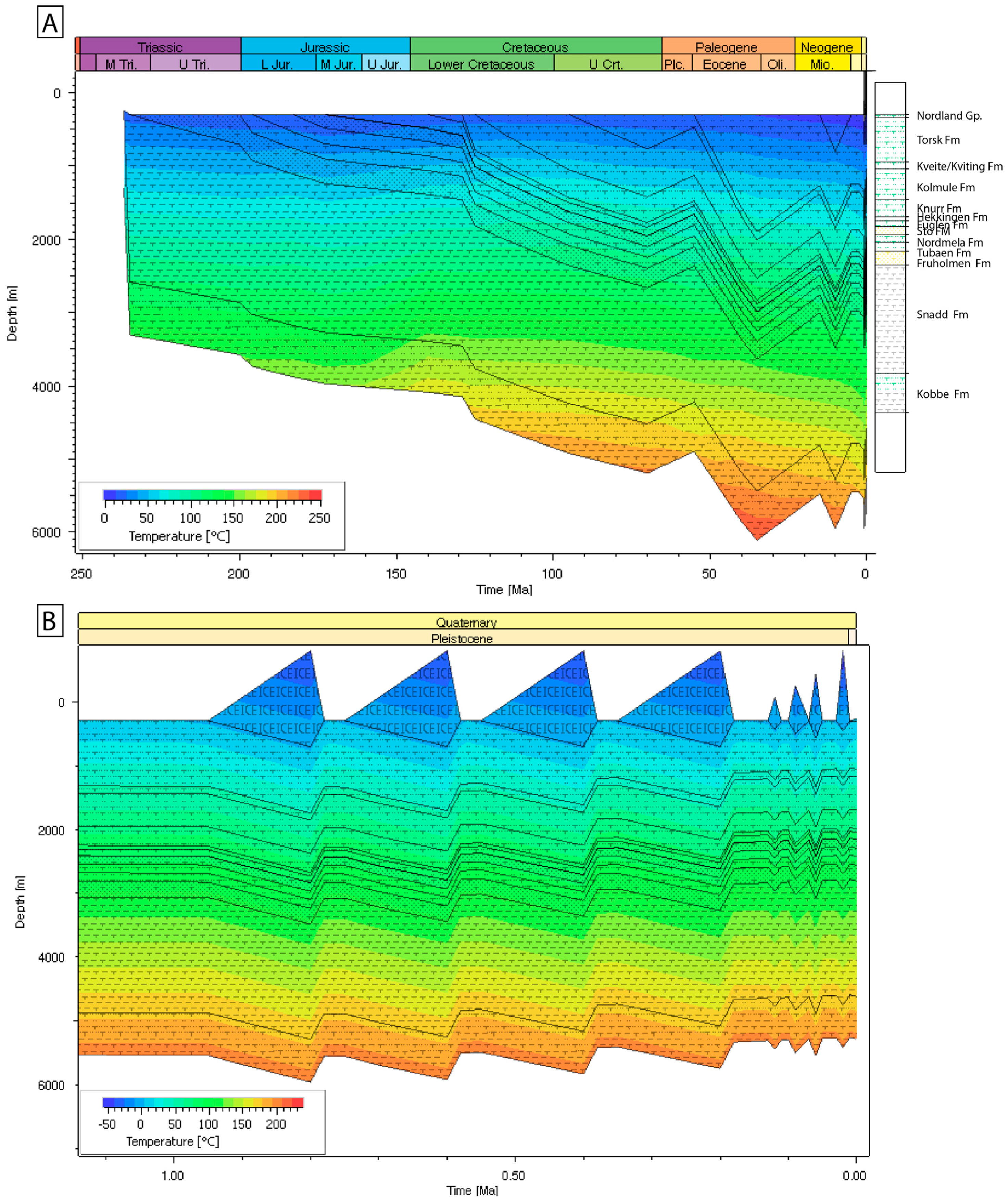
Figure A3.
Model results showing vitrinite reflectance indicating maturity at present-day of the three source rocks (Hekkingen Fm, Kobbe Fm and Snadd Fm).
Figure A3.
Model results showing vitrinite reflectance indicating maturity at present-day of the three source rocks (Hekkingen Fm, Kobbe Fm and Snadd Fm).

Figure A4.
Diagram complimenting Figure 7, showing the pressure plots over geological time showing the fracture gradient of the seals in the model (Fuglen Fm and Hekkingen Fm), as well as pore pressure in the Stø Fm. Note that the pore pressure within Stø Fm does not reach the fracture gradient of the Hekkingen Fm nor the Fuglen Fm. For details of the basin model calibration and setup, see [92].

Figure A5.
Map showing reproduced accumulations, faults and ray tracing migration lines for vapor (red) and for liquid (green). Black lines indicate drainage areas showing hydrocarbon migration into one specific trap as a function of the carried bed [48]. Our predicted values for the gas column are 122 m with a 9-m oil leg. The oil water contact lies at 2404 m, and the gas oil contact lies at 2395 m in our model. Previously reported values by [13] show that the gas water contact is at 2404 m, oil water contact at 2418 m, and the overall gas column is 124 m with an oil leg of 14 m.
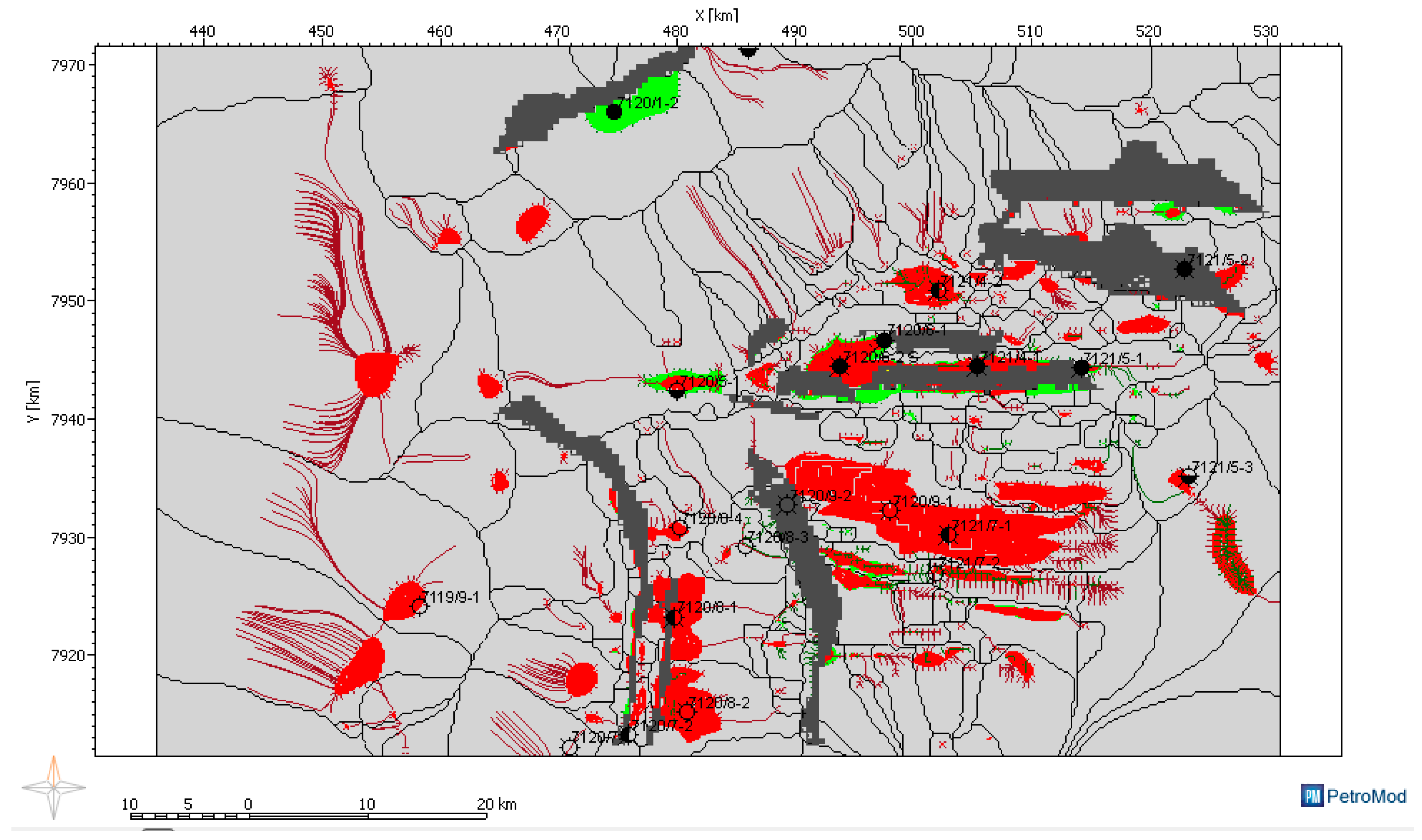
Figure A6.
Table showing the legend accompanying Figure 6 showing the content of the boreholes in comparison to the modelled accumulations.
Figure A6.
Table showing the legend accompanying Figure 6 showing the content of the boreholes in comparison to the modelled accumulations.
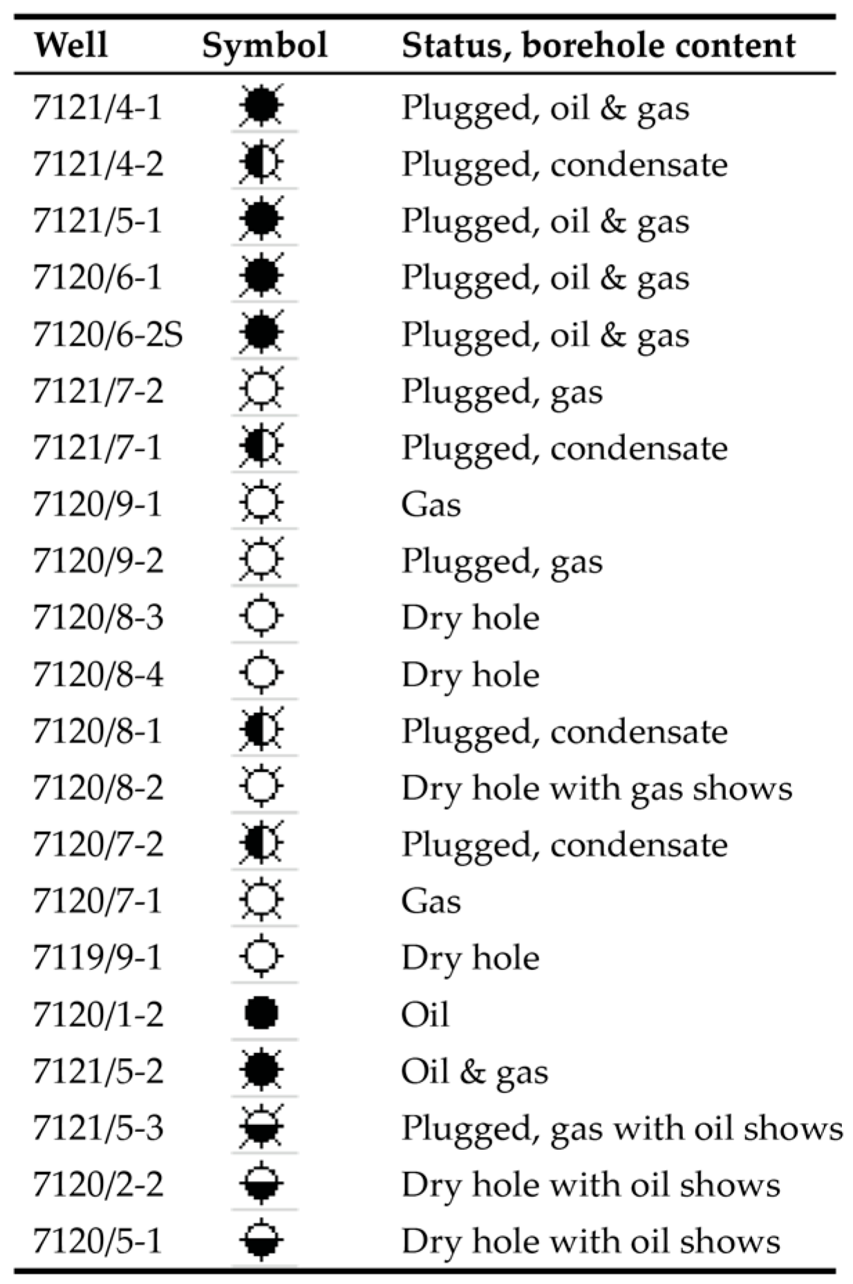
Figure A7.
Cross-sections across the Snøhvit field showing the hydrocarbon migration out of the reservoirs. The red arrows indicate vapor migration vectors, and green lines indicate liquid migration vectors. Note the leakage above the Snøhvit field coinciding with the location of faults (Figure 6).
Figure A7.
Cross-sections across the Snøhvit field showing the hydrocarbon migration out of the reservoirs. The red arrows indicate vapor migration vectors, and green lines indicate liquid migration vectors. Note the leakage above the Snøhvit field coinciding with the location of faults (Figure 6).

References
- Dore, A.G. Barents Sea Geology, Petroleum Resources and Commercial Potential. Arctic 1995, 48, 207–221. [Google Scholar] [CrossRef]
- Doré, A.G. The structural foundation and evolution of Mesozoic seaways between Europe and the Arctic. Palaeogeogr. Palaeoclimatol. Palaeoecol. 1991, 87, 441–492. [Google Scholar] [CrossRef]
- Faleide, J.I.; Tsikalas, F.; Breivik, A.J.; Mjelde, R.; Ritzmann, O.; Engen, O.; Wilson, J.; Eldholm, O. Structure and evolution of the continental margin off Norway and Barents Sea. Episodes 2008, 31, 82–91. [Google Scholar]
- Smelror, M.; Petrov, O.V.; Larsen, G.B.; Werner, S.E. Geological History of the Barents Sea; Geological Survey of Norway: Trondheim, Norway, 2009; 135p. [Google Scholar]
- Ramberg, I.B.; Bryhni, I.; Nottvedt, A.; Rangnes, K. The Making of a Land—The Geology of Norway; Geological Survey of Norway: Trondheim, Norway, 2008; p. 625. [Google Scholar]
- Norwegian Petroleum Directorate (NPD). Available online: http://www.npd.no/en/Topics/ (accessed on 10 December 2016).
- Ohm, S.E.; Karlsen, D.A.; Austin, T.J.F. Geochemically driven exploration models in uplifted areas: Examples from the Norwegian Barents Sea. AAPG Bull. 2008, 92, 1191–1223. [Google Scholar] [CrossRef]
- Estublier, A.; Lackner, A.S. Long-term simulation of the Snøhvit CO2 storage. Energy Procedia 2009, 1, 3221–3228. [Google Scholar] [CrossRef]
- Wennberg, O.P.; Malm, O.; Needham, T.; Edwards, E.; Ottesen, S.; Karlsen, F.; Rennan, L.; Knipe, R. On the occurrence and formation of open fractures in the Jurassic reservoir sandstones of the Snøhvit Field, SW Barents Sea. Pet. Geosci. 2008, 14, 139–150. [Google Scholar] [CrossRef]
- Cavanagh, A.J.; Di Primio, R.; Scheck-Wenderoth, M.; Horsfield, B. Severity and timing of Cenozoic exhumation in the southwestern Barents Sea. J. Geol. Soc. 2006, 163, 761–774. [Google Scholar] [CrossRef]
- Skagen, J.I. Effects on hydrocarbon potential caused by Tertiary uplift and erosion in the Barents Sea. In Artic Geology and Petroleum Potential; Vorren, T.O., Bergsear, E., Dahl-Stammes, O.A., Holter, E., Johansen, B., Lie, E., Lund, T.B., Eds.; Norwegian Petroleum Society Special Publications; Elsevier: Amsterdam, The Netherlands, 1993; Volume 2, pp. 711–719. [Google Scholar]
- Andreassen, K.; Hogstad, K. Gas hydrate in the southern Barents Sea, indicated by a shallow seismic anomaly. First Break 1990, 8, 235–245. [Google Scholar] [CrossRef]
- Linjorded, A.; Grung-Olsen, R. The Jurassic Snøhvit Gas Field, Hammerfest Basin, Offshore Northern Norway. AAPG Mem. 1992, 54, 349–370. [Google Scholar]
- Laberg, J.S.; Andreassen, K. Gas hydrate and free gas indications within the Cenozoic succession of the Bjørnøya Basin, western Barents Sea. Mar. Pet. Geol. 1996, 13, 921–940. [Google Scholar] [CrossRef]
- Chand, S.; Thorsnes, T.; Rise, L.; Brunstad, H.; Stoddart, D.; Bøe, R.; Lågstad, P.; Svolsbru, T. Multiple episodes of fluid flow in the SW Barents Sea (Loppa High) evidenced by gas flares, pockmarks and gas hydrate accumulation. Earth Planet. Sci. Lett. 2012, 331–332, 305–314. [Google Scholar] [CrossRef]
- Ostanin, I.; Anka, Z.; di Primio, R.; Bernal, A. Hydrocarbon plumbing systems above the Snøhvit gas field: Structural control and implications for thermogenic methane leakage in the Hammerfest Basin, SW Barents Sea. Mar. Pet. Geol. 2013, 43, 127–146. [Google Scholar] [CrossRef]
- Ostanin, I.; Anka, Z.; di Primio, R.; Bernal, A. Identification of a large Upper Cretaceous polygonal fault network in the Hammerfest basin: Implications on the reactivation of regional faulting and gas leakage dynamics, SW Barents Sea. Mar. Geol. 2012, 332–334, 109–125. [Google Scholar] [CrossRef]
- Green, P.F.; Duddy, I.R. Synchronous exhumation events around the Arctic including examples from Barents Sea and Alaska North Slope. Geol. Soc. Lond. Pet. Geol. Conf. Ser. 2010, 7, 633–644. [Google Scholar]
- Nyland, B.; Jensen, L.N.; Skagen, J.; Skarpnes, O.; Vorren, T.O. Tertiary uplift and erosion in the Barents Sea—Magnitude, timing and consequences. In Tectonic Modelling and Its Implication to Petroleum Geology; Larsen, R.M., Brekke, H., Larsen, B.T., Talleras, E., Eds.; Norwegian Petroleum Society Special Publications 1; Elsevier: Amsterdam, The Netherlands, 1992; pp. 153–162. [Google Scholar]
- Laberg, J.S.; Andreassen, K.; Vorren, T.O. Late Cenozoic erosion of the high-latitude southwestern Barents Sea shelf revisited. Geol. Soc. Am. Bull. 2012, 214, 77–88. [Google Scholar] [CrossRef]
- Doré, A.G.; Jensen, L.N. The impact of late Cenozoic uplift and erosion on hydrocarbon exploration: Offshore Norway and some other uplifted basins. Glob. Planet. Chang. 1996, 12, 415–436. [Google Scholar] [CrossRef]
- Henriksen, E.; Bjørnseth, H.M.; Hals, T.K.; Heide, T.; Kiryukhina, T.; Kløvjan, O.S.; Larssen, G.B.; Ryseth, A.E.; Rønning, K.; Sollid, K.; et al. Uplift and erosion of the greater Barents Sea: Impact on prospectivity and petroleum systems. Geol. Soc. Lond. Mem. 2011, 35, 271–281. [Google Scholar] [CrossRef]
- Lerche, I.; Yu, Z.; Tørudbakken, B.; Thomsen, R.O. Ice loading effects in sedimentary basins with reference to the Barents Sea. Mar. Pet. Geol. 1997, 14, 277–338. [Google Scholar] [CrossRef]
- Corcoran, D.V.; Dore, A.G. Depressurization of hydrocarbon-bearing reservoirs in exhumed basin settings: Evidence from Atlantic margin and borderland basins. Geol. Soc. Lond. Spec. Publ. 2002, 196, 457–483. [Google Scholar] [CrossRef]
- Zieba, K.J.; Grøver, A. Isostatic response to glacial erosion, deposition and ice loading. Impact on hydrocarbon traps of the southwestern Barents Sea. Mar. Pet. Geol. 2016, 78, 168–183. [Google Scholar] [CrossRef]
- Winsborrow, M.C.M.; Andreassen, K.; Corner, G.D.; Laberg, J.S. Deglaciation of a marine-based ice sheet: Late Weichselian palaeo-ice dynamics and retreat in the southern Barents Sea reconstructed from onshore and offshore glacial geomorphology. Quat. Sci. Rev. 2010, 29, 424–442. [Google Scholar] [CrossRef]
- Rüther, D.C.; Bjarnadóttir, L.R.; Junttila, J.; Husum, K.; Rasmussen, T.L.; Lucchi, R.G.; Andreassen, K. Pattern and timing of the northwestern Barents Sea Ice Sheet deglaciation and indications of episodic Holocene deposition. Boreas 2012, 41, 494–512. [Google Scholar] [CrossRef]
- Siegenthaler, U.; Stocker, T.F.; Monnin, E.; Lüthi, D.; Schwander, J.; Stauffer, B.; Raynaud, D.; Barnola, J.-M.; Fischer, H.; Masson-Delmotte, V.; et al. Stable Carbon Cycle-Climate Relationship During the Late Pleistocene. Science 2005, 310, 1313–1317. [Google Scholar] [CrossRef] [PubMed]
- Rodrigues Duran, E.; di Primio, R.; Anka, Z.; Stoddart, D.; Horsfield, B. 3D-Basin modelling of the Hammerfest Basin (southwestern Barents Sea): A quantitative assessment of petroleum generation, migration and leakage. Mar. Pet. Geol. 2013, 45, 281–303. [Google Scholar] [CrossRef]
- Ostanin, I.; Anka, Z.; di Primio, R.; Bernal, A. Hydrocarbon leakage above the Snøhvit gas field, Hammerfest Basin SW Barents Sea. First Break 2012, 30, 55–60. [Google Scholar] [CrossRef]
- Klitzke, P.; Luzi-Helbing, M.; Schicks, J.M.; Cacace, M.; Jacquey, A.B.; Sippel, J.; Scheck-Wenderoth, M.; Faleide, J.I. Gas Hydrate Stability Zone of the Barents Sea and Kara Sea Region. Energy Procedia 2016, 97, 302–309. [Google Scholar] [CrossRef]
- Tasianas, A.; Mahl, L.; Darcis, M.; Buenz, S.; Class, H. Simulating seismic chimney structures as potential vertical migration pathways for CO2 in the Snøhvit area, SW Barents Sea: Model challenges and outcomes. Environ. Earth Sci. 2016, 75, 1–20. [Google Scholar] [CrossRef]
- Mohammedyasin, S.M.; Lippard, S.J.; Omosanya, K.O.; Johansen, S.E.; Harishidayat, D. Deep-seated faults and hydrocarbon leakage in the Snøhvit Gas Field, Hammerfest Basin, Southwestern Barents Sea. Mar. Pet. Geol. 2016, 77, 160–178. [Google Scholar] [CrossRef]
- Chand, S.; Knies, J.; Baranwal, S.; Jensen, H.; Klug, M. Structural and stratigraphic controls on subsurface fluid flow at the Veslemøy High, SW Barents Sea. Mar. Pet. Geol. 2014, 57, 494–508. [Google Scholar] [CrossRef]
- Gabrielsen, R.H.; Faerseth, R.B.; Jensen, L.N.; Kalheim, J.E.; Riis, F. Structural Elements of the Norwegian Continental Shelf Part 1: The Barents Sea Region; Norwegian Petroleum Directorate Bulletin 6; Norwegian Petroleum Directorate: Stavanger, Norway, 1990; p. 33. [Google Scholar]
- Harland, W.B. The Geology of Svalbard, The Geological Society Memoir No. 17; Geological Society: Bath, UK, 1998; p. 525. [Google Scholar]
- Worsley, D. The post-Caledonian development of Svalbard and the western Barents Sea. Pol. Res. 2008, 27, 298–317. [Google Scholar] [CrossRef]
- Ramberg, I.B.; Bryhni, I.; Nottvedt, A.; Rangnes, K. The Making of a Land—Geology of Norway; Norsk Geologisk Forening (Norwegian Geological Association): Trondheim, Norway, 2008; p. 625. [Google Scholar]
- Knutsen, S.M.; Vorren, T.O. Early Cenozoic Sedimentation In The Hammerfest Basin. Mar. Geol. 1991, 101, 31–48. [Google Scholar] [CrossRef]
- Dalland, W.K. Lithostratigraphic Lexicon of Svalbard. Review and Recommendations for Nomenclature Use. Upper Paleozoic to Quaternary Bedrock; Norsk Polarinstitutt: Tromsø, Norway, 1999; 325 p. [Google Scholar]
- Knies, J.; Matthiessen, J.; Vogt, C.; Laberg, J.S.; Hjelstuen, B.O.; Smelror, M.; Larsen, E.; Andreassen, K.; Eidvin, T.; Vorren, T.O. The Plio-Pleistocene glaciation of the Barents Sea-Svalbard region: A new model based on revised chronostratigraphy. Quat. Sci. Rev. 2009, 28, 812–829. [Google Scholar] [CrossRef]
- Worsley, D.; Johansen, R.; Kristensen, S.E. The Mesozoic and Cenozoic succession of the Tromsoflaket. In A Litho-Stratigraphic Scheme for the Mesozoic and Cenozoic Sucessions Offshore Mid- and Northern Norway; Dalland, A., Worsley, D., Ofstad, K., Eds.; Norwegian Petroleum Directorate (NPD) Bulletin 4; Norwegian Petroleum Directorate: Stavanger, Norway, 1988; Volume 4, pp. 42–65. [Google Scholar]
- Solheim, A.; Kristoffersen, Y. The Physical Environment Western Barents Sea, 1:500000. Sediments above the Upper Regional Unconformity: Thickness, Seismic Stratigraphy and Outline of the Glacial History; Norsk Polarinsitutt Skr.: Tromsø, Norway, 1984; Volume 179B. [Google Scholar]
- Eidvin, T.; Jansen, E.; Riis, F. Chronology of Tertiary fan deposits off the western Barents Sea: Implications for the uplift and erosion history of the Barents Shelf. Mar. Geol. 1993, 112, 109–131. [Google Scholar] [CrossRef]
- Knutsen, S.-M.; Richarden, G.; Vorren, T.O. Late Miocene-Pleistocene sequence stratigraphy and mass-movements on the western Barents Sea margin. In Arctic Geology and Petroleum Potential; Vorren, T.O., Bergsaker, E., Dahl-Stamnes, O.A., Holter, E., Lie, E., Johansen, B., Lund, T.B., Eds.; Norwegian Petroleum Society Special Publications; Elsevier: Amsterdam, The Netherlands, 1992; pp. 573–607. [Google Scholar]
- Berglund, L.T.; Augustson, J.; Faerseth, R.; Gjelberg, J.G.; Ramberg-Moe, H. The evolution of the Hammerfest Basin. In Habitat of Hydrocarbons on the Norwegian Continental Shelf; Graham & Trotman: London, UK, 1986; pp. 319–338. [Google Scholar]
- Vorren, T.O.; Landvik, J.Y.; Andreassen, K.; Laberg, J.S. Glacial History of the Barents Sea Region. In Developments in Quaternary Sciences; Jürgen Ehlers, P.L.G., Philip, D.H., Eds.; Elsevier: Amsterdam, The Netherlands, 2011; Chapter 27; Volume 15, pp. 361–372. [Google Scholar]
- Hantschel, A.; Kauerauf, T. Fundamentals of Basin and Petroleum Systems Modelling; Springer: Berlin/Heidelberg, Germany, 2009. [Google Scholar]
- Siegert, M.J.; Dowdeswell, J.A.; Hald, M.; Svendsen, J.-I. Modelling the Eurasian Ice Sheet through a full (Weichselian) glacial cycle. Glob. Planet. Chang. 2001, 31, 367–385. [Google Scholar] [CrossRef]
- Rüther, D.C.; Mattingsdal, R.; Andreassen, K.; Forwick, M.; Husum, K. Seismic architecture and sedimentology of a major grounding zone system deposited by the Bjørnøyrenna Ice Stream during Late Weichselian deglaciation. Quat. Sci. Rev. 2011, 30, 2776–2792. [Google Scholar] [CrossRef]
- Kukla, G.; Cílek, V. Plio-Pleistocene megacycles: Record of climate and tectonics. Palaeogeogr. Palaeoclimatol. Palaeoecol. 1996, 120, 171–194. [Google Scholar] [CrossRef]
- Svendsen, J.I.; Alexanderson, H.; Astakhov, V.I.; Demidov, I.; Dowdeswell, J.A.; Funder, S.; Gataullin, V.; Henriksen, M.; Hjort, C.; Houmark-Nielsen, M.; et al. Late Quaternary ice sheet history of northern Eurasia. Quat. Sci. Rev. 2004, 23, 1229–1271. [Google Scholar] [CrossRef]
- Sloan, E.D. Clathrate Hydrates of Natural Gases; Marcel Dekker: New York, NY, USA, 1990. [Google Scholar]
- Norwegian Petroleum Directorate (NPD). Norwegian Petroleum Directorate Factmaps. Available online: http://npdmap1.npd.no/website/npdgis/viewer.htm (accessed on 10 June 2011).
- Caine, J.S.; Evans, J.P.; Forster, C.B. Fault zone architecture and permeability structure. Geology 1996, 24, 1025–1028. [Google Scholar] [CrossRef]
- Sibson, R.H. Fluid involvement in normal faulting. J. Geodyn. 2000, 29, 469–499. [Google Scholar] [CrossRef]
- Faulkner, D.R.; Jackson, C.A.L.; Lunn, R.J.; Schlische, R.W.; Shipton, Z.K.; Wibberley, C.A.J.; Withjack, M.O. A review of recent developments concerning the structure, mechanics and fluid flow properties of fault zones. J. Struct. Geol. 2010, 32, 1557–1575. [Google Scholar] [CrossRef]
- Aydin, A. Fractures, faults, and hydrocarbon entrapment, migration and flow. Mar. Pet. Geol. 2000, 17, 797–814. [Google Scholar] [CrossRef]
- Morris, A.; Ferrill, D.A.; Henderson, D.B. Slip-tendency analysis and fault reactivation. Geology 1996, 24, 275–278. [Google Scholar] [CrossRef]
- Freeman, B.; Yielding, G.; Needham, D.T.; Badley, M.E. Fault seal prediction: The gouge ratio method. Geol. Soc. Lond. Spec. Publ. 1998, 127, 19–25. [Google Scholar] [CrossRef]
- Needham, D.T.; Yielding, G.; Freeman, B. Analysis of fault geometry and displacement patterns. Geol. Soc. Lond. Spec. Publ. 1996, 99, 189–199. [Google Scholar] [CrossRef]
- Knipe, R.J. The influence of fault zone processes and diagenesis on fluid flow. In Diagenesis and Basin Development: AAPG Studies in Geology; Horbury, A.D., Robinson, A.D., Eds.; The American Association of Petroleum Geologists: Tulsa, OK, USA, 1993; Volume 36, pp. 135–151. [Google Scholar]
- Fisher, Q.J.; Harris, S.D.; McAllister, E.; Knipe, R.J.; Bolton, A.J. Hydrocarbon flow across faults by capillary leakage revisited. Mar. Pet. Geol. 2001, 18, 251–257. [Google Scholar] [CrossRef]
- Manzocchi, T.; Childs, C.; Walsh, J.J. Faults and fault properties in hydrocarbon flow models. Geofluids 2010, 10, 94–113. [Google Scholar] [CrossRef]
- Sorkhabi, R.; Tsuji, Y. The Place of Faults in Petroleum Traps. In Faults, Fluid Flow, and Petroleum Traps; Sorkhabi, R., Tsuji, Y., Eds.; AAPG Memoir 85; AAPG: Tulsa, OK, USA, 2005. [Google Scholar]
- Sperrevik, S.; Gillespie, P.A.; Fisher, Q.J.; Halvorsen, T.; Knipe, R.J. Empirical estimation of fault rock properties. Nor. Pet. Soc. Spec. Publ. 2002, 11, 109–125. [Google Scholar]
- Ingram, G.M.; Urai, J.L.; Naylor, M.A. Sealing processes and top seal assessment. In Hydrocarbon Seals—Importance for Exploration and Production; Møller-Pedersen, P., Koestler, A.G., Eds.; Norwegian Petroleum Society Special Publications: Trondheim, Norway, 1997; Volume 7, pp. 165–174. [Google Scholar]
- Zatsepin, S.V.; Crampin, S. Modelling the compliance of crustal rock—I. Response of shear-wave splitting to differential stress. Geophys. J. Int. 1997, 129, 477–494. [Google Scholar] [CrossRef]
- Fjeldskaar, W.; Lindholm, C.; Dehls, J.F.; Fjeldskaar, I. Postglacial uplift, neotectonics and seismicity in Fennoscandia. Q. Sci. Rev. 2000, 19, 1413–1422. [Google Scholar] [CrossRef]
- Bjorlykke, K.; Hoeg, K.; Faleide, J.I.; Jahren, J. When do faults in sedimentary basins leak? Stress and deformation in sedimentary basins; examples from the North Sea and Haltenbanken, offshore Norway. AAPG Bull. 2005, 89, 1019–1031. [Google Scholar] [CrossRef]
- Ligtenberg, J.H. Detection of fluid migration pathways in seismic data: Implications for fault seal analysis. Basin Res. 2005, 17, 141–153. [Google Scholar] [CrossRef]
- Wiprut, D.; Zoback, M.D. Fault reactivation and fluid flow along a previously dormant normal fault in the northern North Sea. Geology 2000, 28, 595–598. [Google Scholar] [CrossRef]
- Mattos, N.H.; Alves, T.M.; Omosanya, K.O. Crestal fault geometries reveal late halokinesis and collapse of the Samson Dome, Northern Norway: Implications for petroleum systems in the Barents Sea. Tectonophysics 2016, 690(Part A), 76–96. [Google Scholar] [CrossRef]
- Yielding, G.; Bretan, P.; Freeman, B. Fault seal calibration: A brief review. In Reservoir Compartmentalization; Jolley, S.J., Fisher, Q.J., Ainsworth, R.B., Vrolijk, P.J., Delisle, S., Eds.; Geological Society Special Publications: London, UK, 2010; Volume 347, pp. 243–255. [Google Scholar]
- Dore, A.G.; Corcoran, D.V.; Scotchman, I.C. Prediction of the hydrocarbon system in exhumed basins, and application to the NW European margin. Geol. Soc. Lond. Spec. Publ. 2002, 196, 401–429. [Google Scholar] [CrossRef]
- Grollimund, B.; Zoback, M.D.; Wiprut, D.J.; Arnesen, L. Stress orientation, pore pressure and least principal stress in the Norwegian sector of the North Sea. Pet. Geosci. 2001, 7, 173–180. [Google Scholar] [CrossRef]
- Ekström, G.; Nettles, M.; Abers, G.A. Glacial Earthquakes. Science 2003, 302, 622–624. [Google Scholar] [CrossRef] [PubMed]
- Arvidsson, R. Fennoscandian Earthquakes: Whole Crustal Rupturing Related to Postglacial Rebound. Science 1996, 274, 744–746. [Google Scholar] [CrossRef]
- Stewart, I.S.; Sauber, J.; Rose, J. Glacio-seismotectonics: Ice sheets, crustal deformation and seismicity. Quat. Sci. Rev. 2000, 19, 1367–1389. [Google Scholar] [CrossRef]
- Bolas, H.M.N.; Hermanrud, C.; Teige, G.M.G. The Influence of Stress Regimes on Hydrocarbon Leakage. In AAPG Special Volumes 2005, AAPG Hedberg Series, No. 2: Evaluating Fault and Cap Rock Seals; The American Association of Petroleum Geologists: Tulsa, OK, USA; pp. 109–123.
- Vassenden, F.; Sylta, Ø.; Zwach, C. Secondary migration in a 2D visual laboratory model. In Proceedings of the Conference: Faults and Top Seals, EAGE 2003, Montpellier, France, 8–11 September 2003. [Google Scholar]
- Schowalter, T.T. Mechanics of secondary hydrocarbon migration and entrapment. Am. Assoc. Pet. Geol. Bull. 1979, 63, 723–760. [Google Scholar]
- Fauria, K.E.; Rempel, A.W. Gas invasion into water-saturated, unconsolidated porous media: Implications for gas hydrate reservoirs. Earth Planet. Sci. Lett. 2011, 312, 188–193. [Google Scholar] [CrossRef]
- Bünz, S.; Vadakkepuliyambatta, S.; Mienert, J.; Eriksen, O.K.; Eriksen, F.; Planke, S. P-Cable High-Resolution 3D Seismic Imaging of Hydrate Occurrences over unusually Large Gas Chimneys in the SW Barents Sea. Fire Ice Newsl. 2012, 12, 10–13. [Google Scholar]
- Nickel, J.C.; di Primio, R.; Mangelsdorf, K.; Stoddart, D.; Kallmeyer, J. Characterization of microbial activity in pockmark fields of the SW-Barents Sea. Mar. Geol. 2012, 332–334, 152–162. [Google Scholar] [CrossRef]
- Hermanrud, C.; Halkjelsvik, M.E.; Kristiansen, K.; Bernal, A.; Stromback, A.C. Petroleum column-height controls in the western Hammerfest Basin, Barents Sea. Pet. Geosci. 2014, 20, 227–240. [Google Scholar] [CrossRef]
- Gartrell, A.; Zhang, Y.; Lisk, M.; Dewhurst, D. Enhanced hydrocarbon leakage at fault intersections: An example from the Timor Sea, Northwest Shelf, Australia. J. Geochem. Explor. 2003, 78–79, 361–365. [Google Scholar] [CrossRef]
- Solheim, A.; Elverhøi, A. Gas-related sea floor craters in the Barents Sea. Geo-Mar. Lett. 1993, 13, 235–243. [Google Scholar] [CrossRef]
- Fichler, C.; Henriksen, S.; Rueslaatten, H.; Hovland, M. North Sea Quaternary morphology from seismic and magnetic data: Indications for gas hydrates during glaciation? Pet. Geosci. 2005, 11, 331–337. [Google Scholar] [CrossRef]
- Lerche, I.; Bagirov, E. Guide to gas hydrate stability in various geological settings. Mar. Pet. Geol. 1998, 15, 427–437. [Google Scholar] [CrossRef]
- Judd, A.G.; Hovland, M. Seabed Fluid Flow; Cambridge University Press: Cambridge, UK, 2007; p. 476. [Google Scholar]
- Ostanin, I. Hydrocarbon Plumbing Systems and Leakage Phenomenon in the Hammerfest Basin, Southwest Barents Sea. Ph.D. Thesis, Technical University Berlin, Berlin, Germany, 2015. [Google Scholar]
Figure 1.
(A) Location of the study area, Greater Barents Sea, offshore Norway. (B) Structural map of the SW Barents Sea; RLFC: Ringvassøy-Loppa Fault Complex; AFC: Asterias Fault Complex; TFFC: Troms/Finnmark Fault Complex; BFC: Bjørnøyrenna Fault Complex. Key faults that were mapped were included in a large regional basin model, which includes the Snøhvit, Snøhvit North, Snøhvit Beta, Albatross and Askeladd fields and their kitchen areas. The higher resolution nested model includes the Snøhvit and Albatross fields.
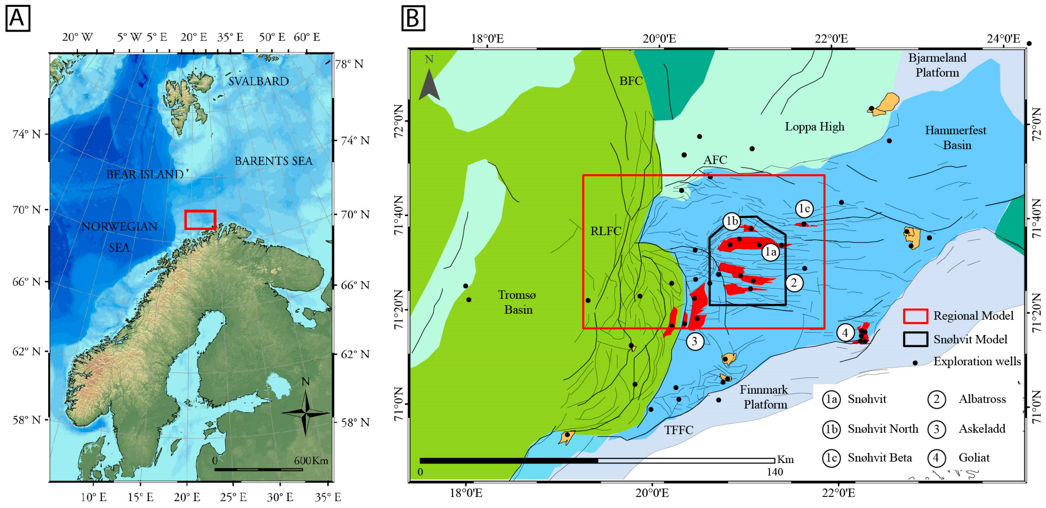
Figure 2.
(A) Two-way travel time (TWT) structure map of the Stø reservoir. Location of the gas chimney outline is highlighted together with well locations. (B) Interpreted cross-section of the stratigraphy (modified from [13,17]) showing the structural setting and the main stratigraphic units of the Stø reservoir. The EW trending faults bounding the Snøhvit field have been repeatedly reactivated [17] and penetrate the sequences from Triassic up to the Paleocene-Early Eocene Torsk Formation.
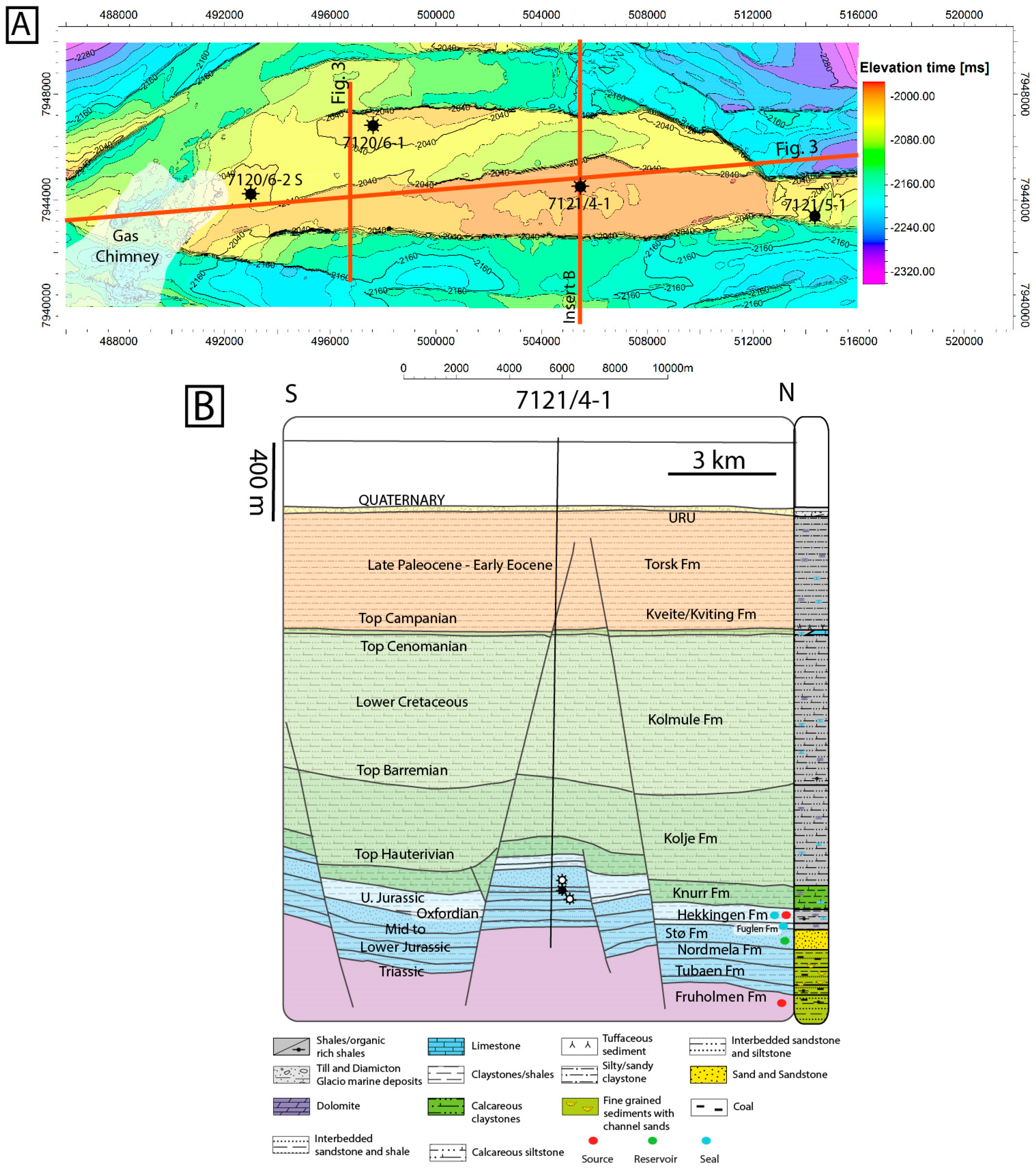
Figure 3.
Seismic cross-sections across the Snøhvit field with key stratigraphic units that were used to build the 3D petroleum systems model (see Figure 2 for the location). Reactivated first order faults penetrate the reservoirs linking to the Cenomanian-Campanian polygonal fault interval and reactivated polygonal faults in the Paleocene-Early Eocene. The location of the Bottom Simulating Reflector (BSR) above the gas chimney is shown together with the timing of fault activity and hydrocarbon generation from key source rocks. PFs: Polygonal Faults.

Figure 4.
(A) 3D visualization of an interpreted regional EW trending fault through the Jurassic reservoir up to the shallow subsurface, crosscutting a BSR, linking with shallow faults, overlain by buried and present-day seabed pockmarks. (B) Example of the BSR reflector, cross-cut by reactivated polygonal faults with fluid flow pipes above, leading to buried pockmarks on the Upper Regional Unconformity (URU) and seabed pockmarks (for details, see Figure 5 and [16]).

Figure 5.
(A) 3D block interpretation of the Albatross field and the deep Jurassic faults, Cenomanian-Campanian polygonal faults and the reactivated polygonal faults overlain by mega pockmarks on the seabed and the URU. (B) Example of buried pockmarks on the URU surface in the area above the BSR (modified from [16]).
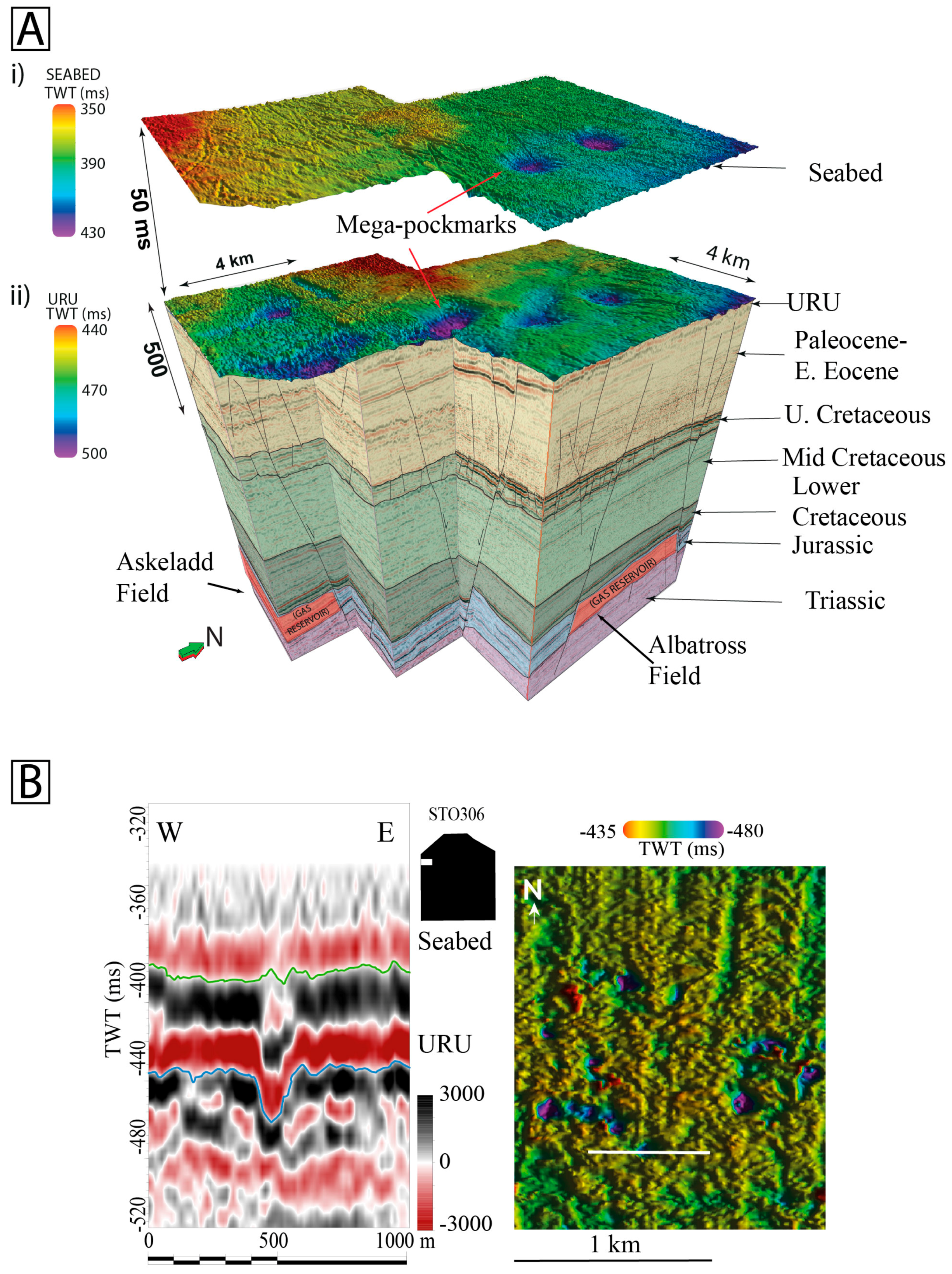
Figure 6.
Modelled accumulations based on 3D petroleum system modelling showing the main Snøhvit, Albatross and Askeladd reservoirs, as well as associated oil and gas phases. Input fault traces are also shown, as well as petroleum break-through locations, based on maximum hydrocarbon (HC) column height, reservoir structure and sealing capacity [48]. The insert (bottom left) shows the location and outlines of discoveries and producing fields in the Hammerfest Basin; the Snøhvit discovery is a gas field with an oil leg [6]. Figure A6 documents the hydrocarbon phase relationships of proven discoveries.

Figure 7.
Results of the 3D petroleum systems model. (A) Temperature profile at the top of the ice sheet during the last 1.2 Ma. (B) Pressure profiles of the Stø reservoir during the last 1.2 Ma. (C) Accumulated hydrocarbon mass in the Snøhvit reservoir. Loss of mass is shown as a function of changing fault properties. (D) Hydrocarbon mass outflow at the top of the model, as a function of changing fault properties. White areas represent times of glacial loading, and vertical grey zones represent deglaciation events.
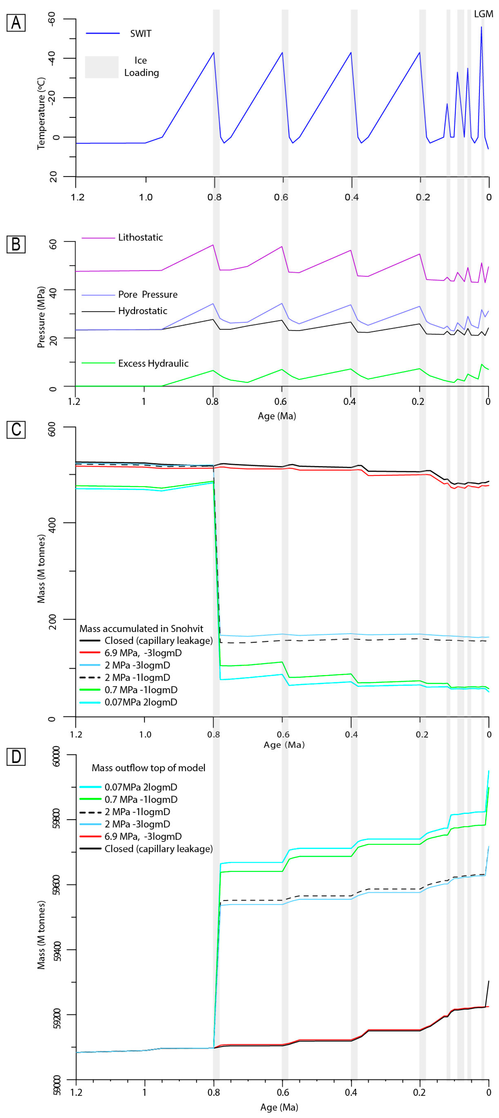
Figure 8.
(A) Display of the interpreted faults bounding the Snøhvit field together with hydrocarbon leakage indicators (gas chimney, BSR, enhanced reflections (see Figure 4)). (B) Representative results of the nested model at 200 m × 200 m for closed faults during glaciations. (C) Conducting faults during deglaciation. Fault plane color scale displays hydrocarbon saturation, based on locations of break-throughs, calculated from column heights, trap geometry and seal capillary entry pressure (for details, see [48]). During glaciations when faults are closed, no break-throughs occur along Fault B (insert in (B)). Once the faults become conductive, hydrocarbons migrate vertically along the fault plane, then laterally upon reaching less resistive strata (lower capillary entry pressure and permeability) and then vertically to the shallow strata (Figure A7) once another cell with lower capillary entry pressure and permeability is reached (insert in (C)).
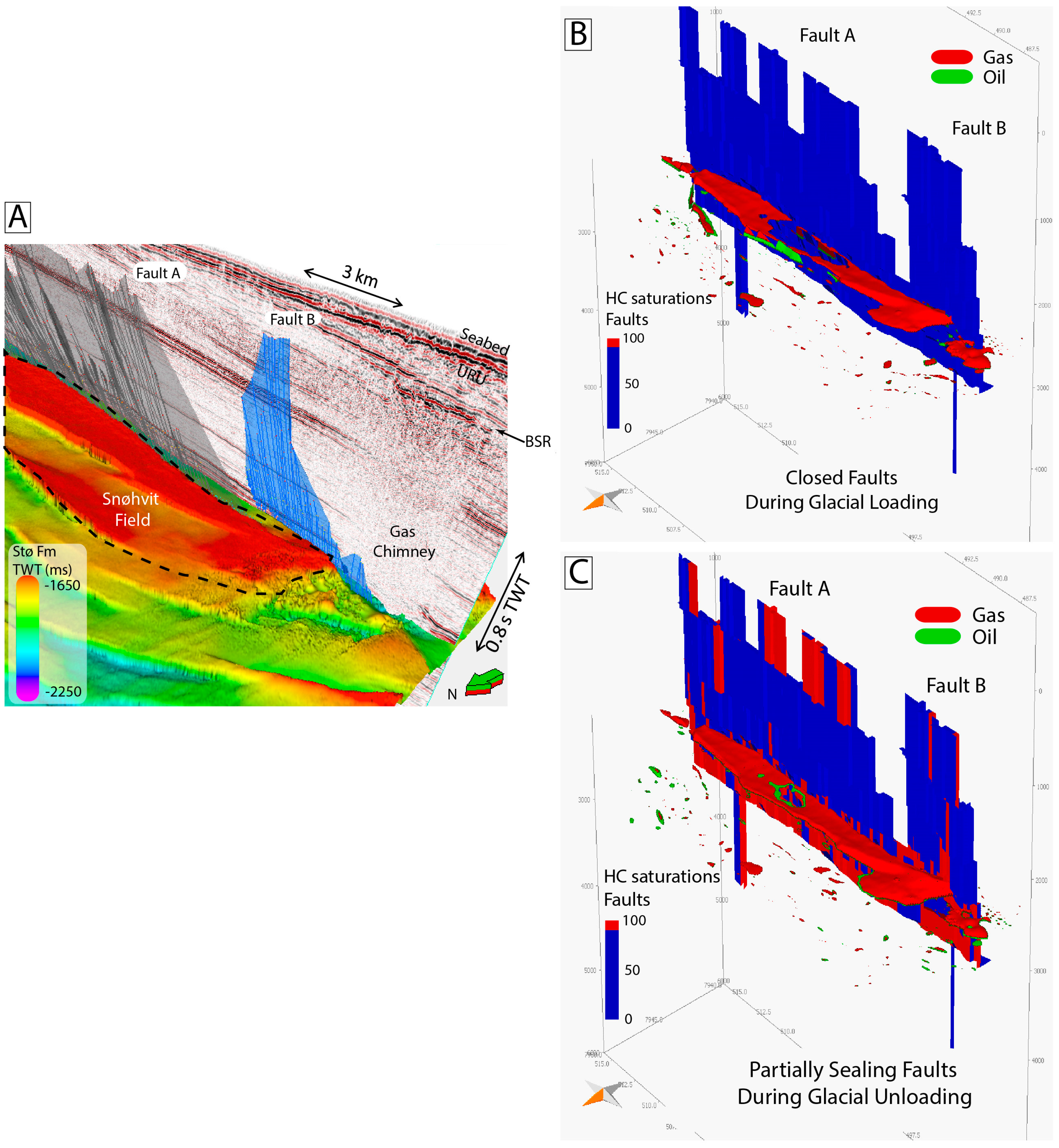
Figure 9.
Present day accumulations in the Jurassic Stø formation showing: (A) petroleum migration flow paths (based on ray tracing [48] into the structures (see Figure A5)), as well as (B) a well section profile across the Snøhvit reservoir showing the location of the principal EW trending fault and the relative depths of the reservoirs. Insert in (A) shows that hydrocarbons migrate from the northern kitchen area into Snøhvit North, then Snøhvit, and the break-through locations (see Figure 6) indicate a leakage point, which is marked by a dashed circle. Hydrocarbons then flow into the Albatross field structure up dip. Askeladd field sees a different charge direction from the deeper Tromsø Basin in the west (see Figure 1).

Figure 10.
Conceptual model of leakage from the Hammerfest Basin including gas hydrate stability phase diagrams. Phase diagrams are adapted from [16]. ICE: the thickness of the Barents Sea Ice Sheet at time of glaciations; GHSZ: Gas Hydrate Stability Zone (denoted by the BSR); GOC: Gas Oil Contact; OWC: Oil Water Contact. (A) Initial reservoir filling, followed by initial glacial loading (older than URU, >0.8 Ma); (B) recorded fluid escape event on URU, ca. 0.8 Ma; (C) Weichselian glaciations; (D) tilting following the Last Glacial Maximum and last fluid flow event recorded on the seabed.


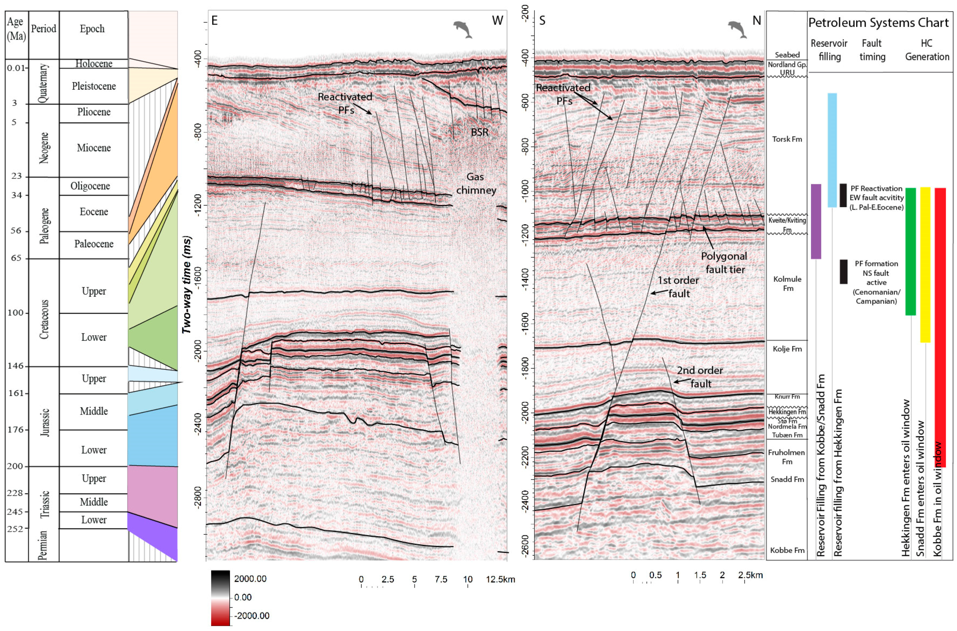
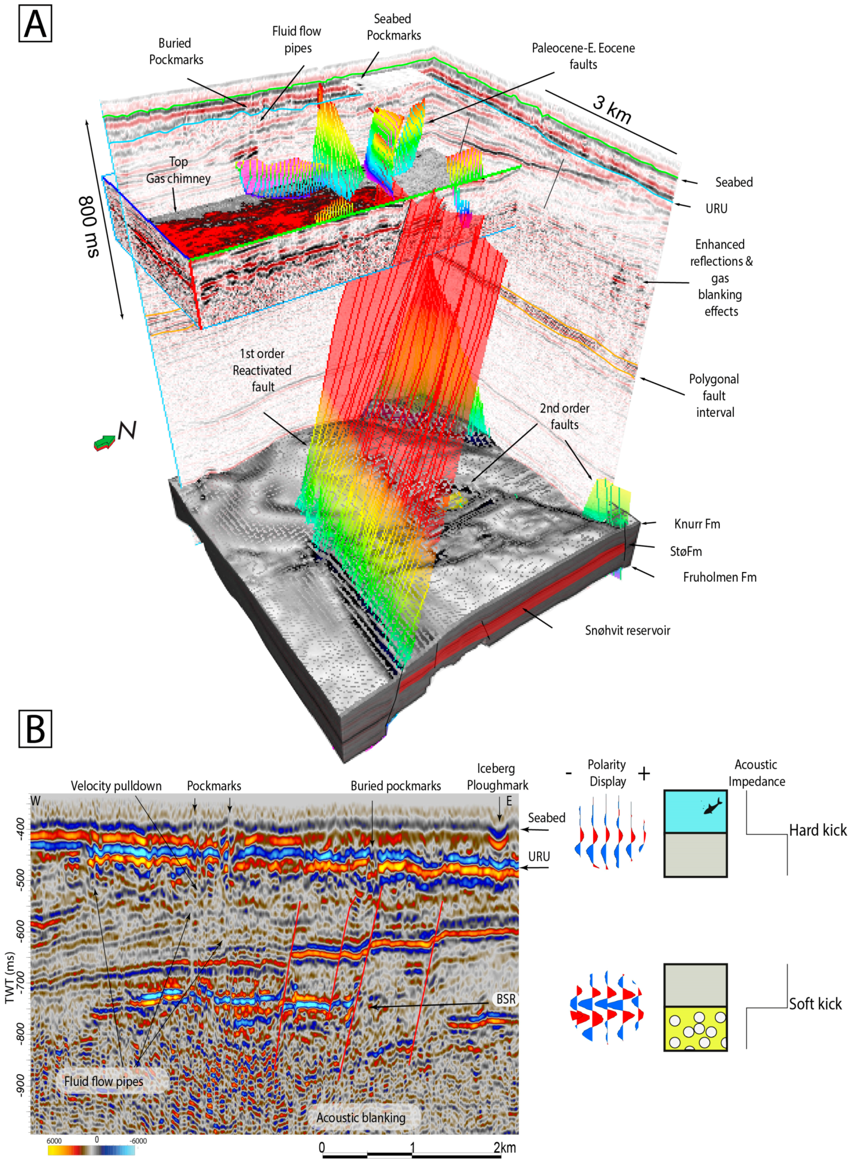
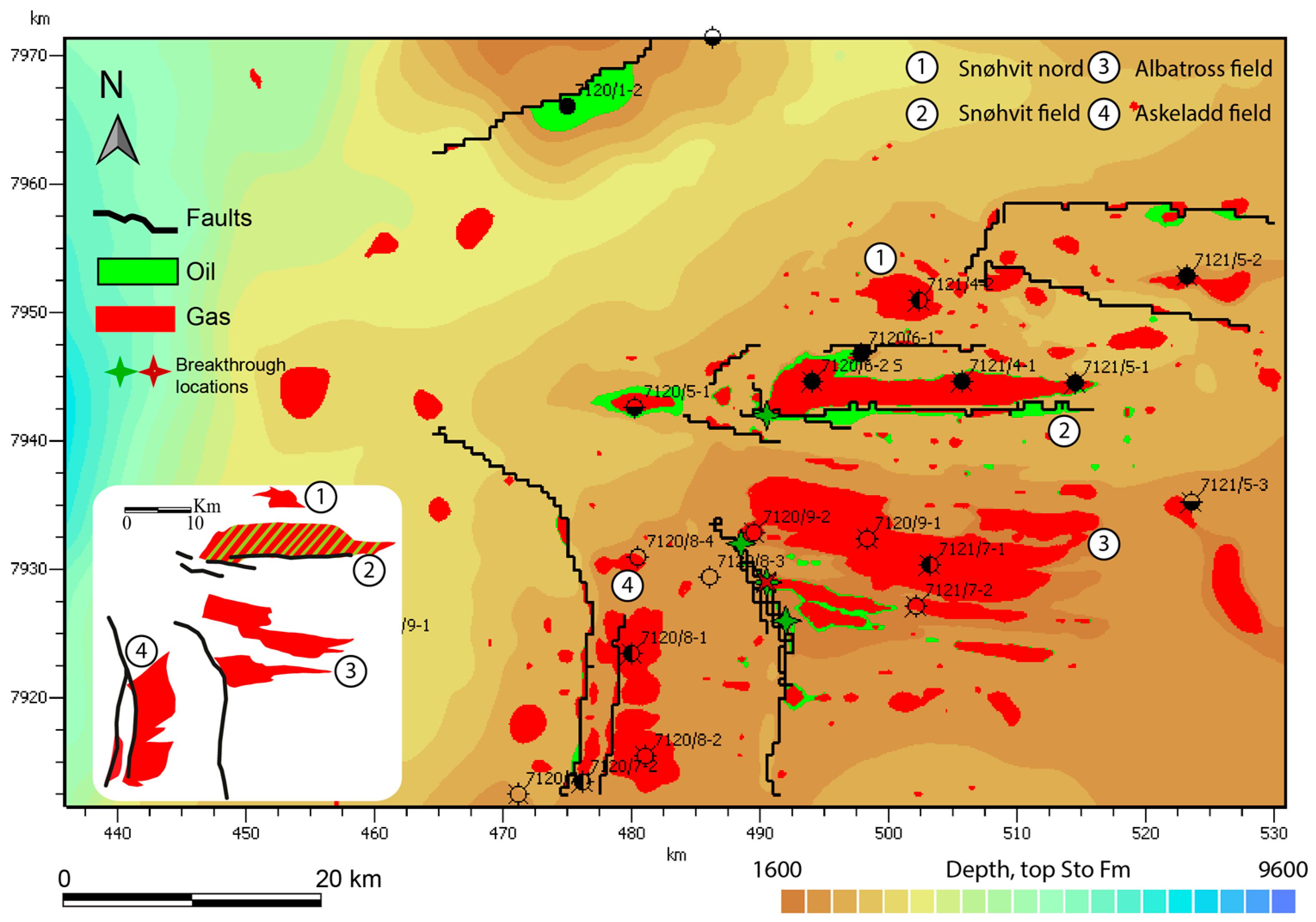
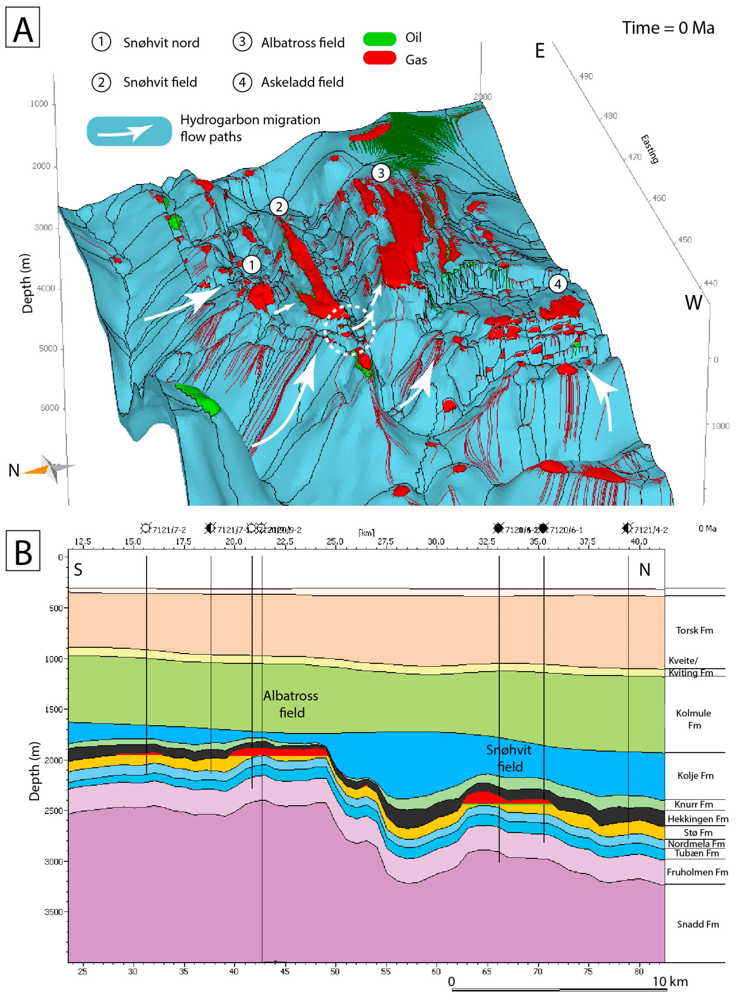
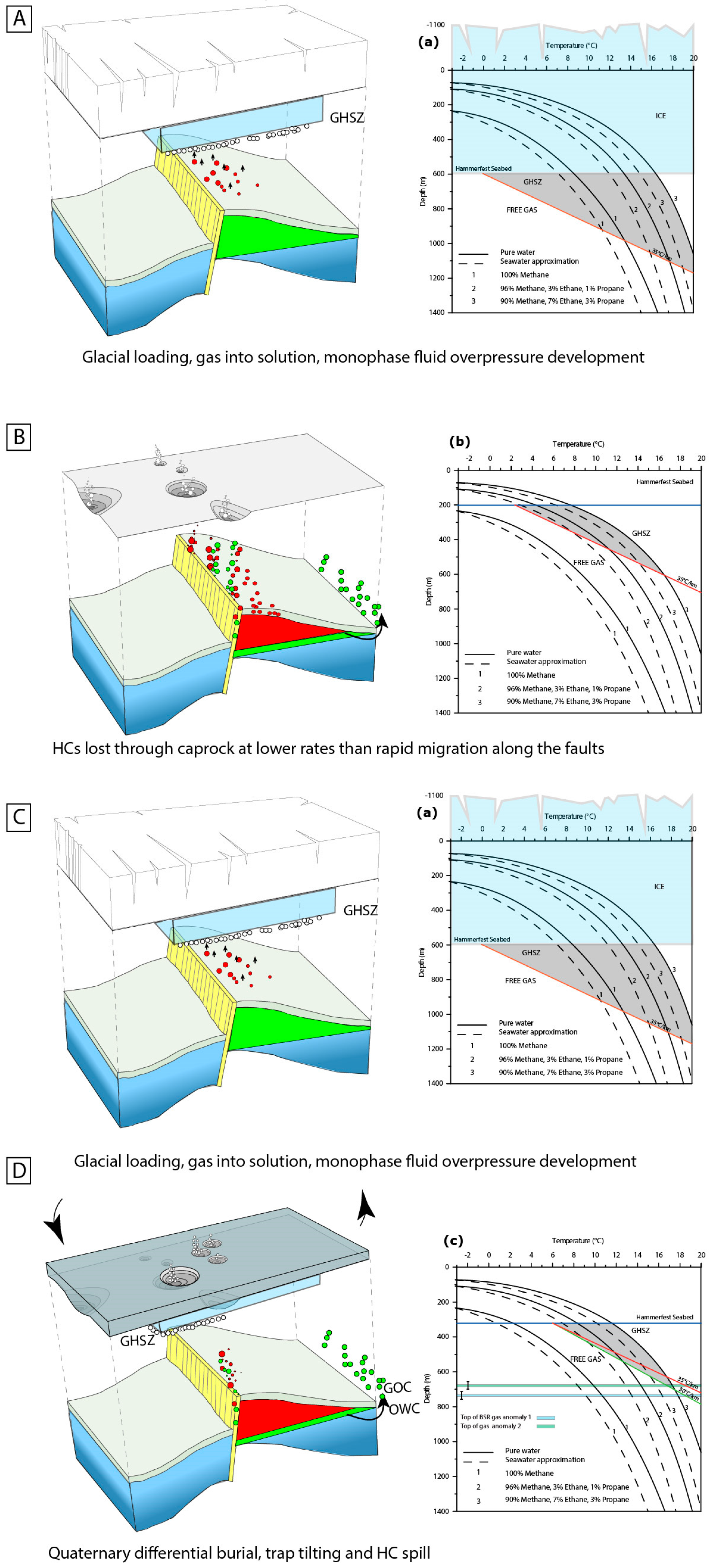
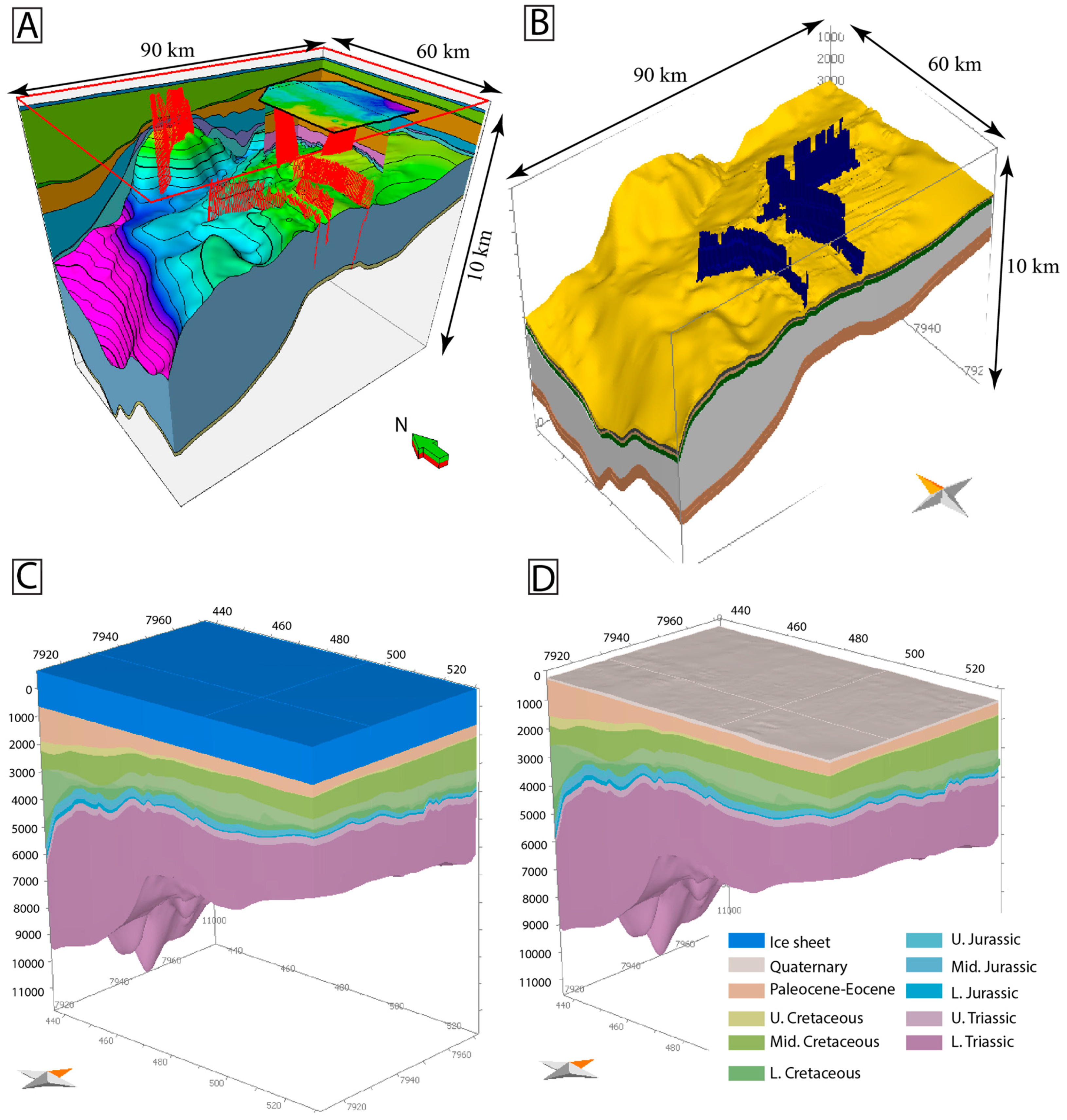
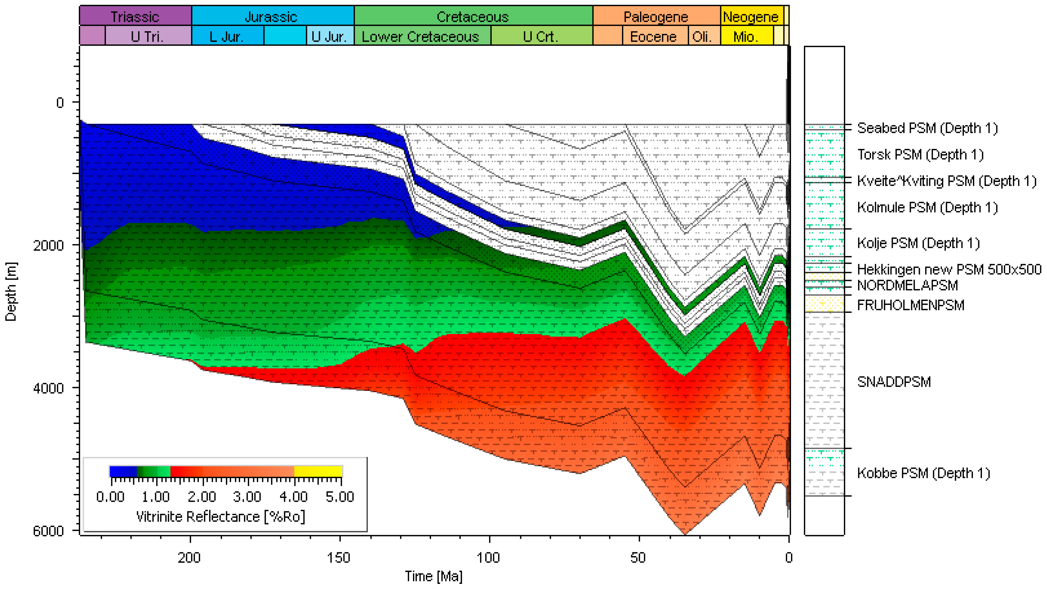
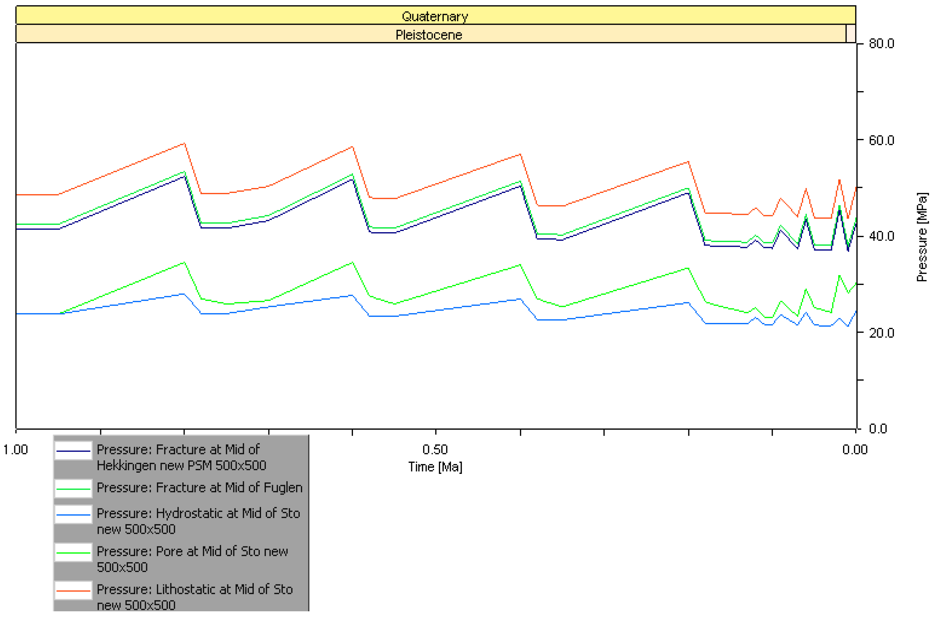
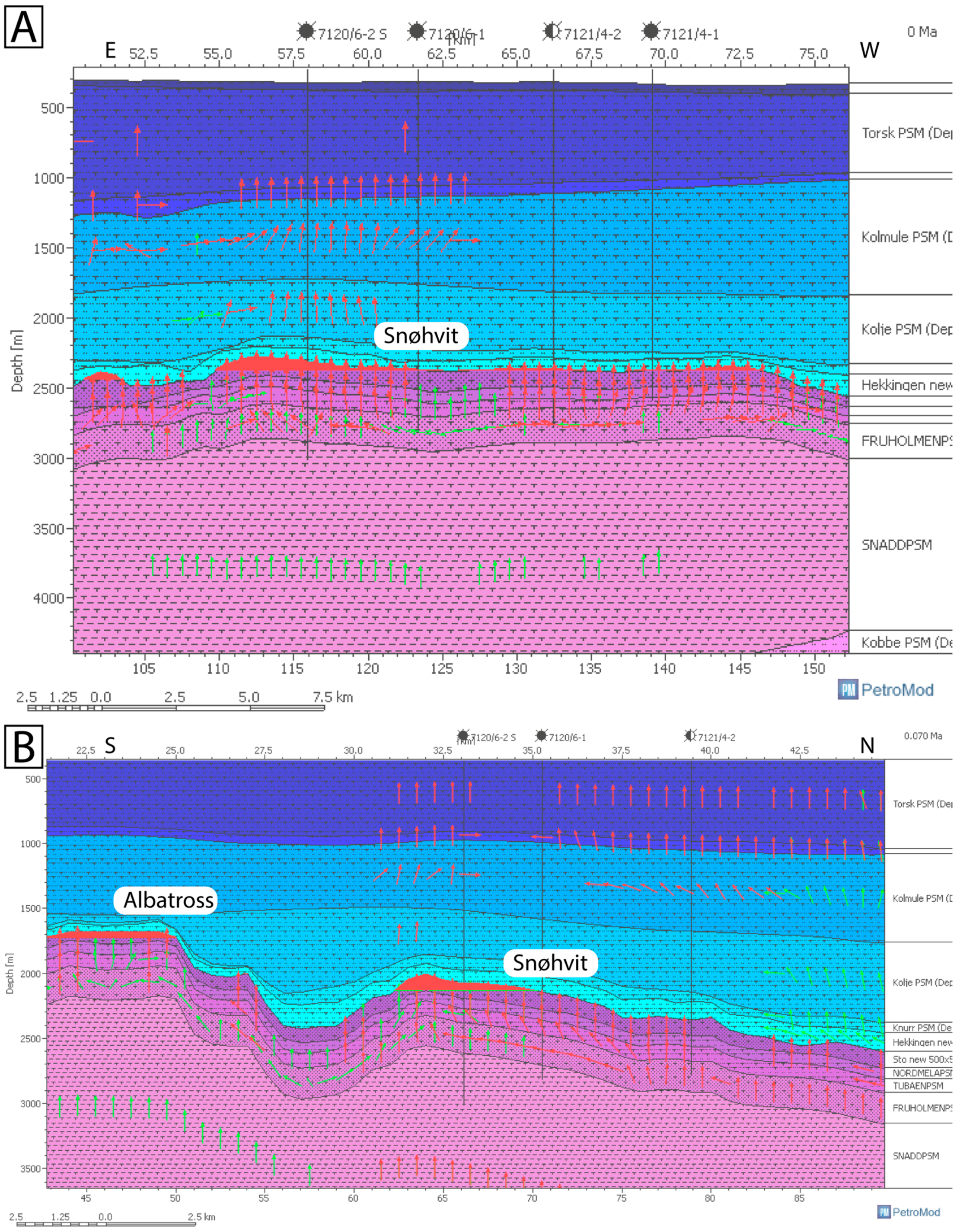
Table 1.
Defined fault properties for the petroleum system model sensitivity runs based on the empirical relationship for the capillary entry pressure for fault rocks [66,67]. Each FCP value was tested having a permeability assigned to it according to the data spread of [66,67].
| FCP * | Permeability (log mD **) | Permeability (mD **) |
|---|---|---|
| Closed | - | - |
| 6.9 | −3 | 0.001 |
| 2 | −3 | 0.001 |
| 2 | −1 | 0.1 |
| 0.7 | −1 | 0.1 |
| 0.07 | 2 | 100 |
* FCP: Fault Capillary entry Pressure in MPa; ** mD: millidarcy.
Table 2.
Input boundary conditions for the timing of fault dilation and fault sealing during the glacial-interglacial periods.
Table 2.
Input boundary conditions for the timing of fault dilation and fault sealing during the glacial-interglacial periods.
| Conductive Faults | Closed Faults | ||
|---|---|---|---|
| Age * from | Age up to | Age From | Age up to |
| 0.8 | 0.78 | 150 | 0.8 |
| 0.6 | 0.58 | 0.78 | 0.6 |
| 0.4 | 0.38 | 0.58 | 0.4 |
| 0.2 | 0.18 | 0.38 | 0.2 |
| 0.12 | 0.11 | 0.18 | 0.12 |
| 0.09 | 0.07 | 0.11 | 0.09 |
| 0.06 | 0.05 | 0.07 | 0.06 |
| 0.02 | 0 | 0.05 | 0.02 |
* Age in Ma.
© 2017 by the authors. Licensee MDPI, Basel, Switzerland. This article is an open access article distributed under the terms and conditions of the Creative Commons Attribution (CC BY) license (http://creativecommons.org/licenses/by/4.0/).
Share and Cite
MDPI and ACS Style
Ostanin, I.; Anka, Z.; Di Primio, R. Role of Faults in Hydrocarbon Leakage in the Hammerfest Basin, SW Barents Sea: Insights from Seismic Data and Numerical Modelling. Geosciences 2017, 7, 28. https://doi.org/10.3390/geosciences7020028
AMA Style
Ostanin I, Anka Z, Di Primio R. Role of Faults in Hydrocarbon Leakage in the Hammerfest Basin, SW Barents Sea: Insights from Seismic Data and Numerical Modelling. Geosciences. 2017; 7(2):28. https://doi.org/10.3390/geosciences7020028
Chicago/Turabian StyleOstanin, Ilya, Zahie Anka, and Rolando Di Primio. 2017. "Role of Faults in Hydrocarbon Leakage in the Hammerfest Basin, SW Barents Sea: Insights from Seismic Data and Numerical Modelling" Geosciences 7, no. 2: 28. https://doi.org/10.3390/geosciences7020028
Note that from the first issue of 2016, this journal uses article numbers instead of page numbers. See further details here.