Three-Dimensional Geologic Model of Glacial Outwash in Mclean County, Illinois, Based on Seismic Refraction Studies

Abstract

Seven two-dimensional (2-D) seismic refraction lines were used to determine the thickness and geometry of a valley train outwash deposit of the Quaternary Henry Formation near Heyworth in southern McLean County, Illinois. These refraction data were collected and processed in 2-D, then imported into a Petrel, a three-dimensional (3-D) geological modeling software package. The 3-D geologic model was built using the velocity attribute of the seismic refraction data. The 3-D velocity model was then verified manually by moving a cross-section through the velocity model at 20 m increments. These selected data points were used to create 3-D horizons, surfaces, and contacts constraining the target Henry Formation from the overlying alluvium of the Cahokia Formation and the underlying Delavan Till. Results of the 3-D model show the Henry Formation outwash trends about S10°E, which is oblique to S55°W-trending modern Kickapoo Creek valley. The Henry Formation outwash is confined to the Kickapoo valley, and consists of well-stratified sand and gravel at that is as much as 25 m in thickness in the channel. The thickness of the Henry Formation in the terrace is 8–10 m. The Cahokia Formation is everywhere about 2 m in thickness. The Henry Formation here is interpreted to be deposited in a subglacial tunnel valley that was deposited about 20,000 years ago as the Laurentide ice sheet retreated from its maximum southerly extent.

1. Introduction

The principal question addressed with this research is: What is the 3-D architecture of the Henry Formation valley-train outwash near Heyworth, Illinois? We answered this question by shooting multiple refraction lines across and around the perimeter of the study site that allowed us too: (1) identify the location and trend of the valley train throughout the study site in 2-D; (2) construct a 2.5-D model allowing for the correlation and calibration of each line to one another and a borehole drilled at the center of the study site (BH01); (3) create a 3-D geologic model using Petrel to determine the volume of the deposit; and (4) propose an interpretation of the genesis of the Henry Formation in this area.

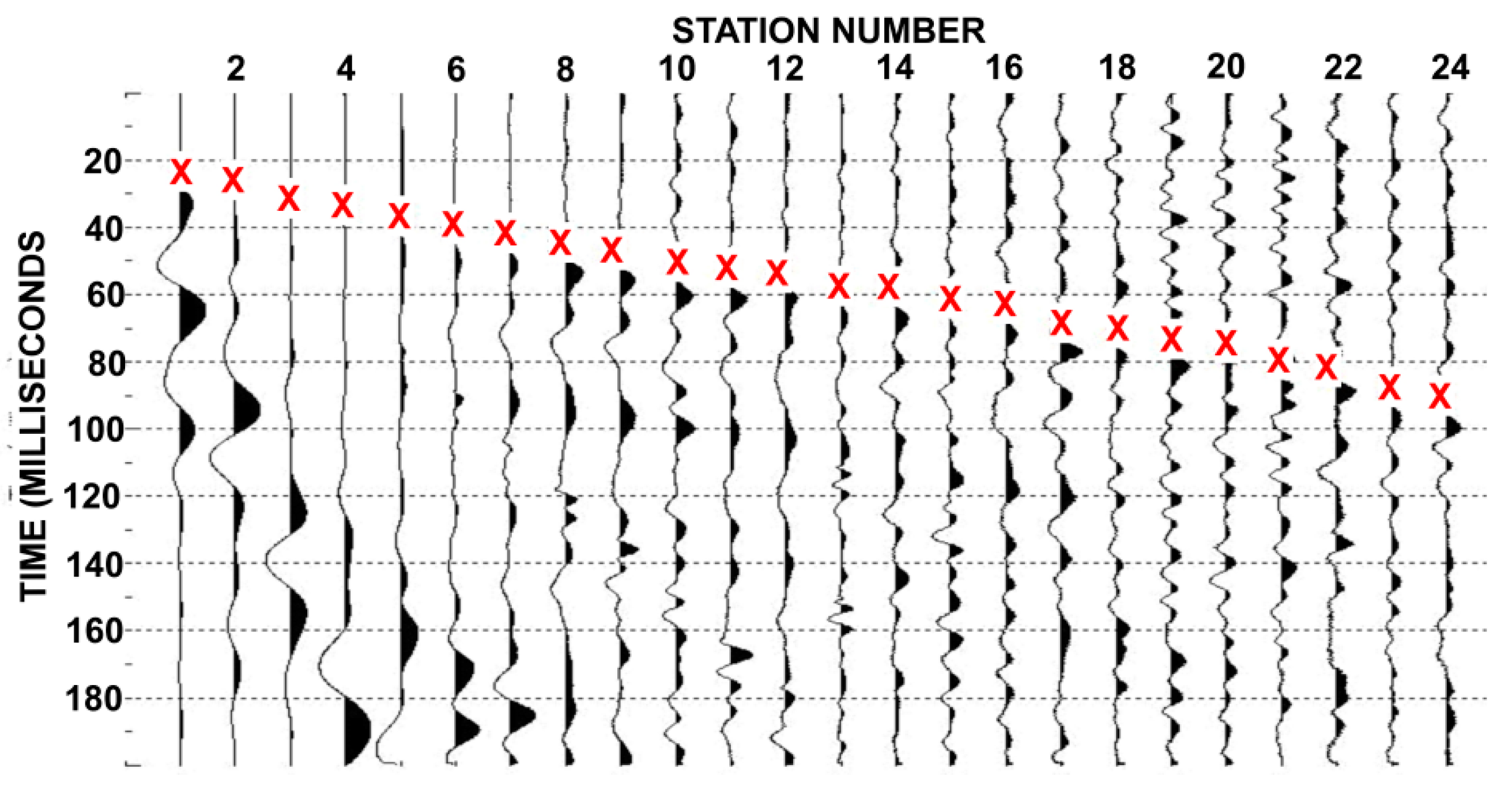
Seismic refraction tomography utilizes travel-time inversion of seismic waves transmitted through geologic materials. Seismic waves refract when crossing lithologic layers with different seismic velocities, sending out “wavelets” that are then recorded as vertical offset by a string of geophones. Of the various shallow geophysical methods available (e.g., GPR, reflection seismology, resistivity etc.), seismic refraction requires less cost and time in data acquisition and processing [1]. Limitations of refraction seismology include velocity inversions, missing layers and decreased depth penetration with a given energy source [2]. Because the units within this study area are flat-lying and have only two targeted refractors confining the unit of interest, refraction seismology is ideal for this shallow subsurface investigation because an increasing velocity gradient is expected.

Our methods are novel, in that the refraction velocity data in itself is imported into Petrel for the construction of the 3-D geologic model. This is a distinctly different approach than determining the elevations of reflectors and then inserting these data as points into the modeling software.

2. Previous Research

Seismic refraction is widely used throughout the geoscience industries, and has been proven to be a reliable means of imaging the subsurface. Avalos [3] used the same equipment and methodologies used in this research to map the bedrock topography beneath a gravel and peat marginal marine succession in southwest Devon, UK. More commonly, other geophysical methods such as seismic reflection [4], ground penetrating RADAR [5,6] or a combination of geophysical methods [7] are used to image glacial sand and gravel deposits.

3. Geologic Setting

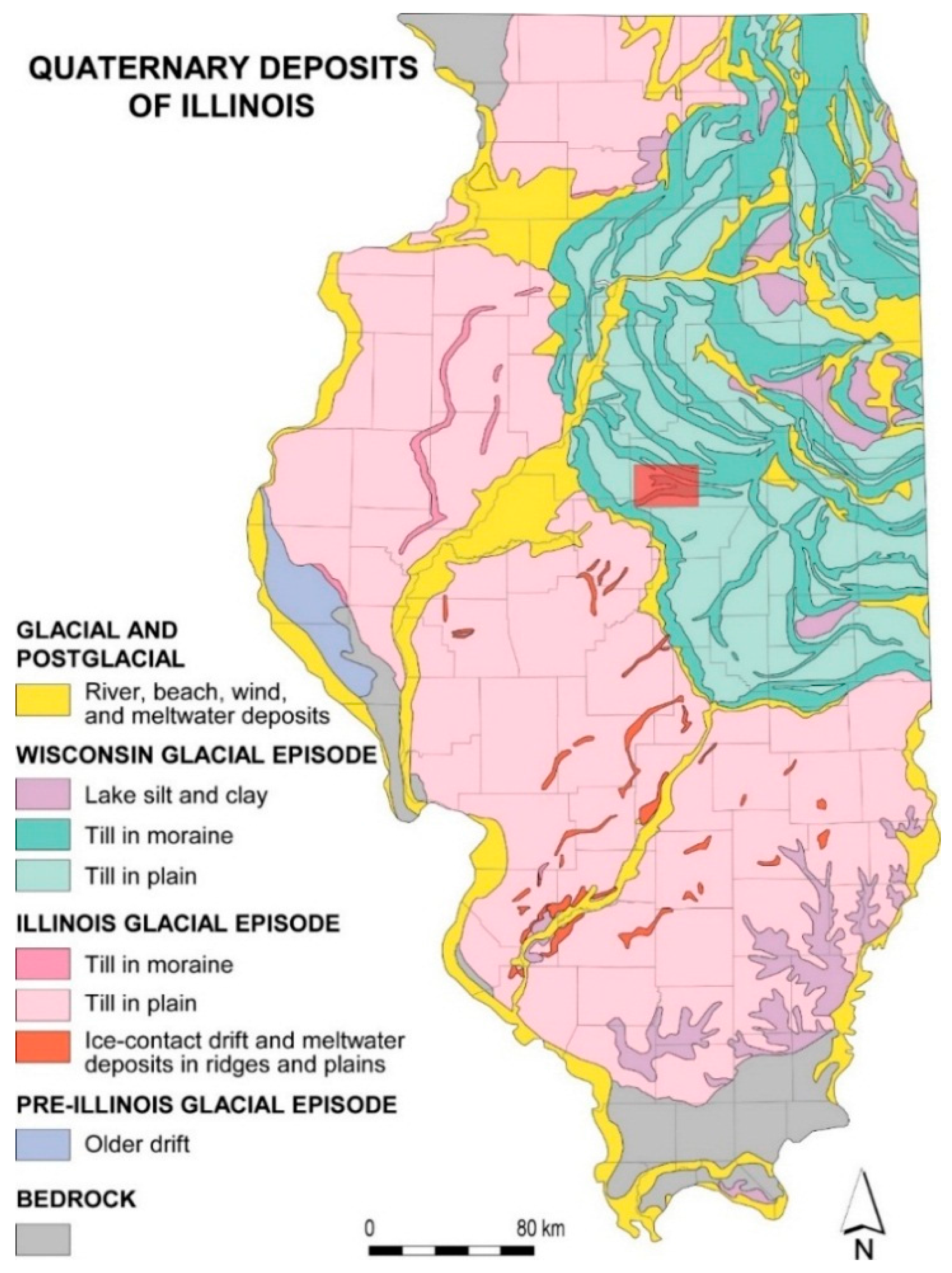
Petternson et al. [8] describes the dynamics of the Larentide ice sheet during the Wisconsin glacial episode (Figure 1, [9]). The southern edge of the Laurentide ice sheet formed several lobes flowing southward along the regional topographic lows of the north-central United States. These Wisconsin ice sheets migrated into Illinois between 14,000 and 23,000 years ago. As the Lake Michigan Lobe went through a series of advances and retreats, numerous end and recessional moraines developed. An end moraine system developed in Mclean County (Figure 2), in which melting ice provided large quantities of sediment and water [10]. A valley train is defined as outwash that occurs within the confines of a stream valley downstream of melting ice [11,12].

Figure 1. Surficial geologic map of Illinois showing the distribution of Quaternary glacial deposits. The area portrayed in Figure 2 is indicated by the blue box. Map is modified from: ISGS Staff, 2005, Quaternary deposits: Illinois State Geological Survey, ISGS 8.5 × 11 map series.

Figure 1. Surficial geologic map of Illinois showing the distribution of Quaternary glacial deposits. The area portrayed in Figure 2 is indicated by the blue box. Map is modified from: ISGS Staff, 2005, Quaternary deposits: Illinois State Geological Survey, ISGS 8.5 × 11 map series.

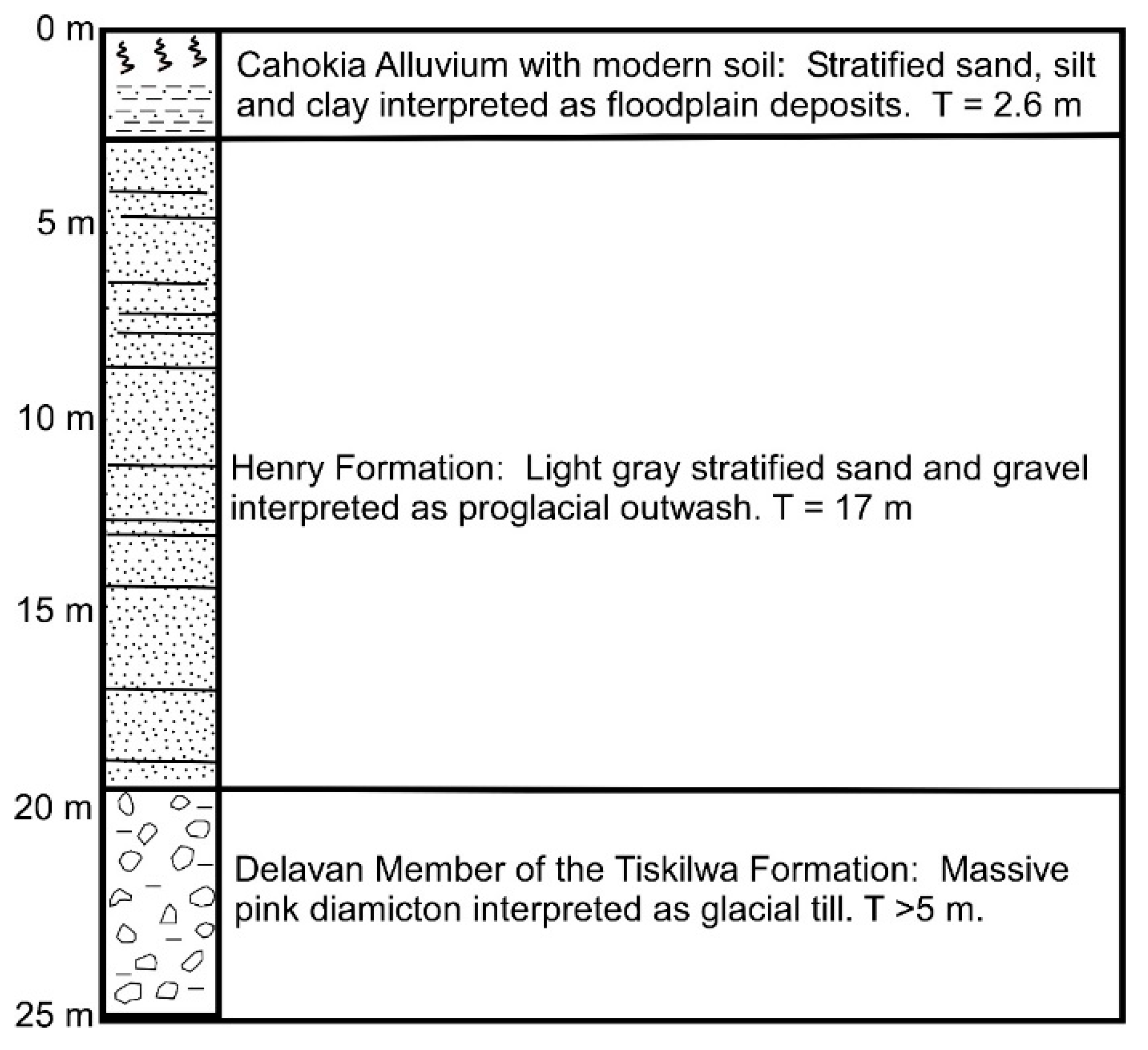
The Henry Formation is part of the Mason Group and is comprised of poorly sorted, sub-angular, stratified, course sand and gravel [13] that was deposited by melt-out events during the Wisconsin episode of glaciation. The Henry Formation varies from ~10–25 m in thickness in the study area.

The Henry Formation is overlain by Holocene alluvium of the Cahokia Formation; it overlies the Delavan Till (Tiskilwa Formation, Wedron Group) a pink to gray diamicton deposited during the Wisconsin glacial episode [14]. The Delavan is the oldest of the Wisconsin episode tills in Illinois.

Hansel and Johnson [13] describe three members (or more appropriately three facies) of the Henry Formation. The Wasco Member is the coarsest facies, consisting largely of gravel, and occurs as melt-out landforms such as kames or eskers. The Batavia Member is more variable in texture, and occurs as outwash plains, most typically along the down-ice side of a recessional moraine. The Mackinaw Member, which is what is present in the study area, is the finest-grained of the three members, and consists of sand, pebbly sand and gravel. The Mackinaw Member was deposited as a “valley train”, which means that the sediments are localized to stream valleys. These valley-train deposits were deposited either as meltwater streams south of the melting ice or subglacial tunnel valleys.

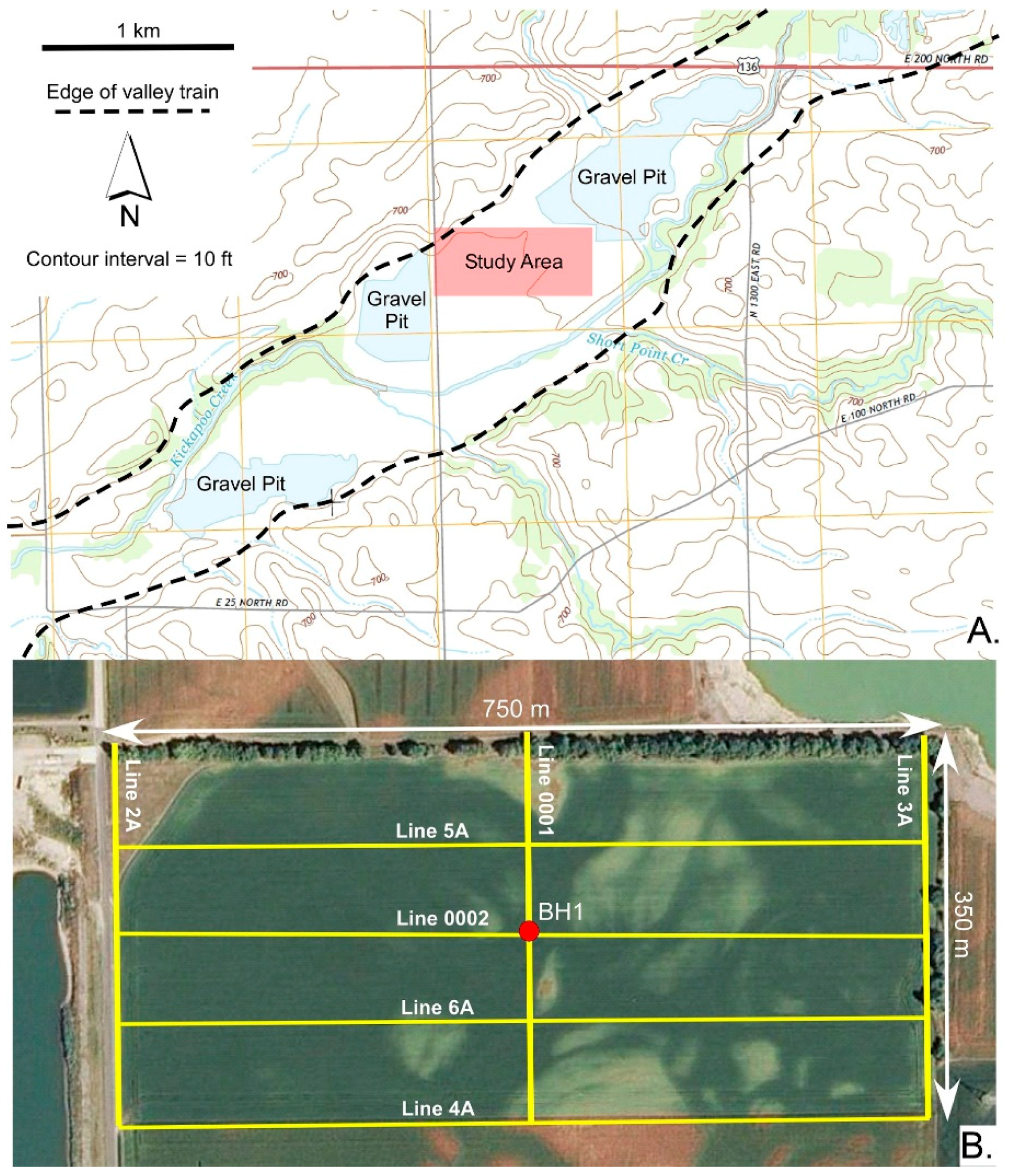
This study was conducted about 3 km west of Heyworth, IL (Figure 3). The study site is located among active sand/gravel pits, and is approximately 350 m by 700 m. in area, The property owner, who is interested in the volume of the Henry Formation on this property for possible pit development, had Testing Service Corporation (TSC) drill a borehole at the intersection of Line 0001 and Line 0002 (BH01). Figure 4 is the log of the sediment core of BH01. The ISGS has multiple public access well records for wells located in adjacent areas. These data are available as part of the ILWATER database. The borehole and water well data were used in the construction of the 3D geologic model.

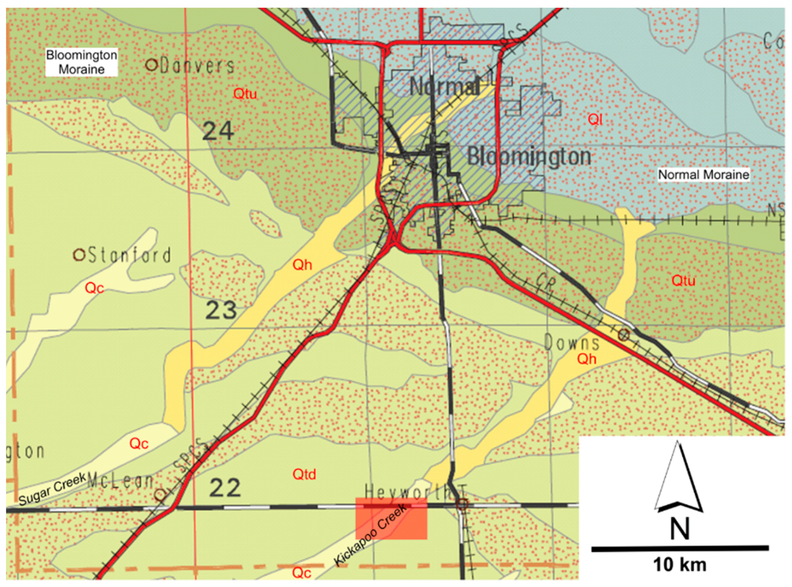
Figure 2. Surficial geologic map of southern McLean County, IL (modified from Stiff et al. [9]). This area is dominated by Wisconsin age glacial deposits that form recessional moraine and till plain landforms. Qtd = Tiskilwa Formation, Delavan Member, Qh = Henry Formation. The area of Figure 3A is indicated by the red box.

Figure 2. Surficial geologic map of southern McLean County, IL (modified from Stiff et al. [9]). This area is dominated by Wisconsin age glacial deposits that form recessional moraine and till plain landforms. Qtd = Tiskilwa Formation, Delavan Member, Qh = Henry Formation. The area of Figure 3A is indicated by the red box.

Figure 3. (A) Topography map of the Kickapoo Creek valley west of Heyworth, IL that indicates the study area and the outline of the valley train outwash deposit; (B) Air photo of the study area indicating the seismic profile shot lines. The yellow lines are the locations of the seismic profiles. The borehole is indicated by BH01.

Figure 3. (A) Topography map of the Kickapoo Creek valley west of Heyworth, IL that indicates the study area and the outline of the valley train outwash deposit; (B) Air photo of the study area indicating the seismic profile shot lines. The yellow lines are the locations of the seismic profiles. The borehole is indicated by BH01.

Figure 4. Lithologic log of sediments present in BH01.

Figure 4. Lithologic log of sediments present in BH01.

4. 2-D Seismic Refraction Methods

4.1. Data Collection

Using Seistronix RAS-24 remote acquisition system, we shot three N-S and four E-W seismic refraction profiles. Seismic energy was generate by sledge hammer strikes on a steel plate. The lateral resolution of refraction surveys is one half the geophone spacing, and the survey depth resolution is one quarter the spread length. With a geophone spacing of 5 m and spread length of 120 m, the lateral resolution is 2.5 m with depth capabilities of about 30 m. To gain adequate coverage beneath the first and last geophones, we overlapped each spread by 30 m. This allowed geophones in each consecutive spread to receive multiple shots to each station (Figure 5). Narwold and Owen [15] state that the overlap of each geophone spread presents the illusion of both forward and reverse seismic origins, which allows the processing software to interpret the overlap as if the spreads were a single line. This aids in modeling velocity differences in case of high-noise environments. Shots were taken and recorded every two stations beginning at 30 m before the first geophone, and 25 m beyond the last geophone, which provided six overlapping shots from set locations along the previous spread. Lankston [16] demonstrated that by taking shots every other station (Figure 6), the processing software will account for depth in the Z rather than X direction.

Figure 5. Coverage profile based on number of front and reverse wave crossovers. The red and yellow zones occur in areas were the most shots and wave path crossovers occurred.

Figure 5. Coverage profile based on number of front and reverse wave crossovers. The red and yellow zones occur in areas were the most shots and wave path crossovers occurred.

Figure 6. Initial 1-D gradient model. This model is in Surfer 8 as a base model prior to the ray-tracing feature that occurs during the tomographic processing. The x-axis represents distance along the seismic line in meters.

Figure 6. Initial 1-D gradient model. This model is in Surfer 8 as a base model prior to the ray-tracing feature that occurs during the tomographic processing. The x-axis represents distance along the seismic line in meters.

4.2. Processing

The seismic data was processed in the Rayfract 3.14 software package, which enables the development of an inverted model. The WET (Wavepath eikonal traveltime inversion) process allows for the development of accurate models without running hundreds of iterations (Min and Shin, [17]. Rayfract 3.14 processing software uses first break energy and wave propagation in conjunction with wave paths to generate tomographic images created through an iterative process (Figure 7).

Figure 7. “Shot gather” screen shot from Rayfract 3.14. First break picking: Red X: Software picks used to create lowest RMS error from wave crossover distances after 20 WET iterations.

Figure 7. “Shot gather” screen shot from Rayfract 3.14. First break picking: Red X: Software picks used to create lowest RMS error from wave crossover distances after 20 WET iterations.

First a 1-D minimum structure velocity profile is created from the refraction travel time data. This initial 1-D model is the basis for warping the tomographic images to derive the most likely ray path. Schuster [18] advocates the WET method because of its computationally efficient inversion scheme in the space-time domain. This system of inversions is as effective as the Wavepath Travel time (WT) inversion and is much faster. Unlike ray-tracing tomography, WET partially accounts for band-limited source and shadow effects in the data reducing effects of small lithologic velocity inversions.

4.3. Velocity Calibration

The choice of the borehole location was designed to achieve proper calibration without the additional expense of multiple boreholes. After the data were collected, calibration of each line to one another was determined through processing with multiple iterations and using velocity variations to define each contact. Calibration of the velocity models for Line 0001 and Line 0002 achieved the appropriate soil thickness of 2.6 m, as evidenced in BH01, using a velocity of 750 m/s. The base of the sand and gravel unit was achieved using a velocity of 1975 m/s., which agrees with the depth to the base of the sand and gravel evident in BH01. This velocity is consistent with the results of Pavlovic [19], who demonstrated that velocities of clay-based materials vary between 1200 and 2500 m/s. Each of the three stratigraphic units are present in each velocity profile.

5. Seismic Refraction Results

For each of the seven interpreted seismic profiles, “sand and gravel” refers to outwash of the Henry Formation; “diamictite” refers to the Delavan Till. The base of the Henry Formation occurs to a depth of at least 10 m throughout the study area. In many areas, the contact is flat at this 10 m depth. Thus, this depth is referred to descriptively as the “terrace” level. Depths lower than 10 m is referred to descriptively as “channel”. Line 0001 and Line 0002 were shot in early March. The rest of the profiles were shot in April. The base of the Cahokia Alluvium in Line 0001 is spurious, perhaps because the frost was not entirely out of the ground when these data were gathered. For each profile, shots were taken for 25 m on either side of the first and last geophones in the array to increase resolution.

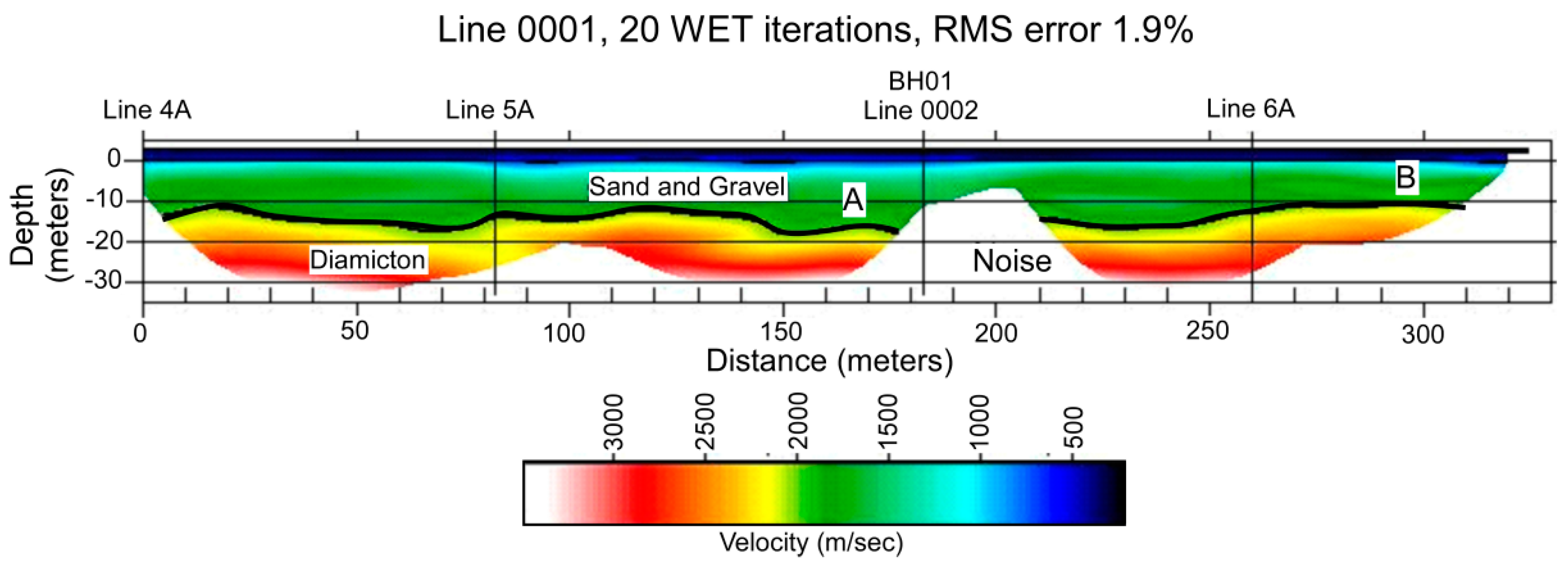
Line 0001 (Figure 8) is a north-south velocity profile that runs through the central part of the study areal. Like the rest of the north-south profiles, Line 0001 is comprised of three 24-geophone lines, with a geophone spacing of 5 m resulting in a 120 m spread. Along Line 0001, the channel depth varies between ~10–19 m. Here the channel base is non-distinct. It is broadly undulating and runs from the south end of the profile to the 260 m distance point.

Figure 8. North-South velocity profile through Line 0001, which runs through the center of the study area. South is to the left. Here the channel is non-distinct, and runs from the about 20–260 m from the south end of the profile and is not more than 20 m deep. A = channel; B = terrace.

Figure 8. North-South velocity profile through Line 0001, which runs through the center of the study area. South is to the left. Here the channel is non-distinct, and runs from the about 20–260 m from the south end of the profile and is not more than 20 m deep. A = channel; B = terrace.

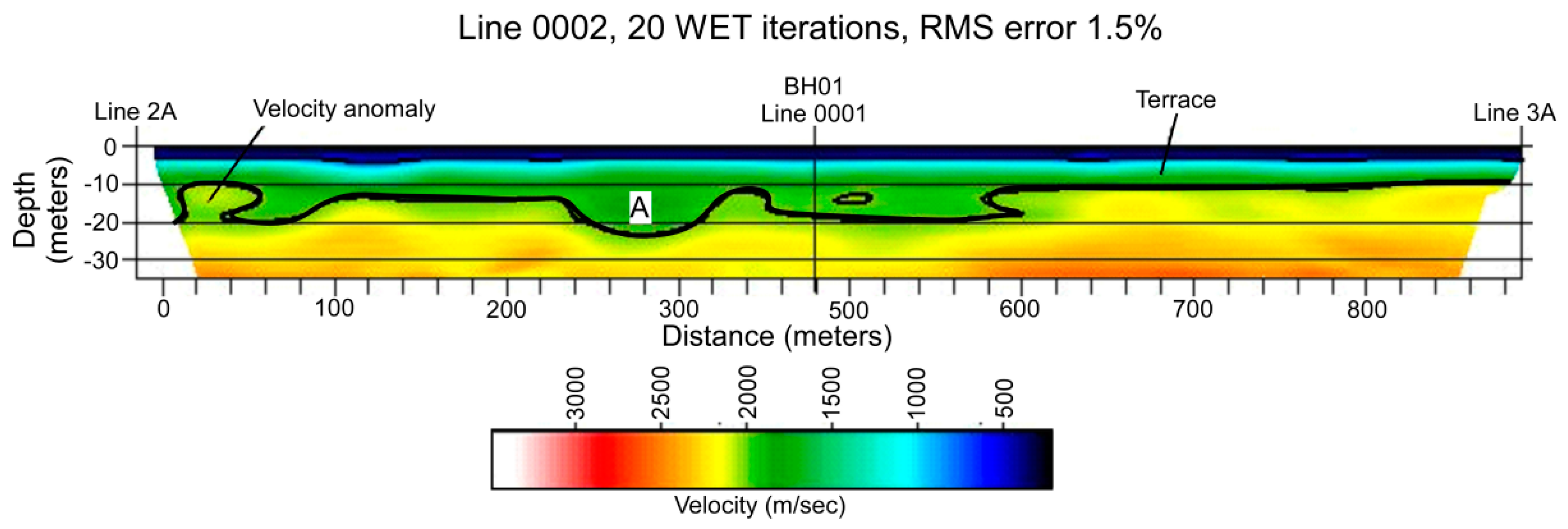
Line 0002 (Figure 9) is an east-west velocity profile that runs through the central part of the study area. Like the rest of the east-west profiles, Line 0002 is comprised of seven 24-geophone lines, with a 2 geophone overlap. Here the channel is well defined, and runs from 220 to 580 m from the west end of the section. Within the channel, the deepest part (indicated by A in Figure 9) reaches a depth of about 22 m. There is a velocity anomaly at the west end of the profile, which may represent a second channel. It may also represent disturbed ground related to the construction of the county road. The terrace is clearly defined at a depth of 10 m, and runs from the 600 m distance to the east end of the profile.

Figure 9. East-West seismic velocity profile of Line 0002, which runs through the central part of the study area. West is to the left. The terrace is indicated, as it the deepest part of the channel (indicated by A). The velocity profile at the west end of the profile also is noted.

Figure 9. East-West seismic velocity profile of Line 0002, which runs through the central part of the study area. West is to the left. The terrace is indicated, as it the deepest part of the channel (indicated by A). The velocity profile at the west end of the profile also is noted.

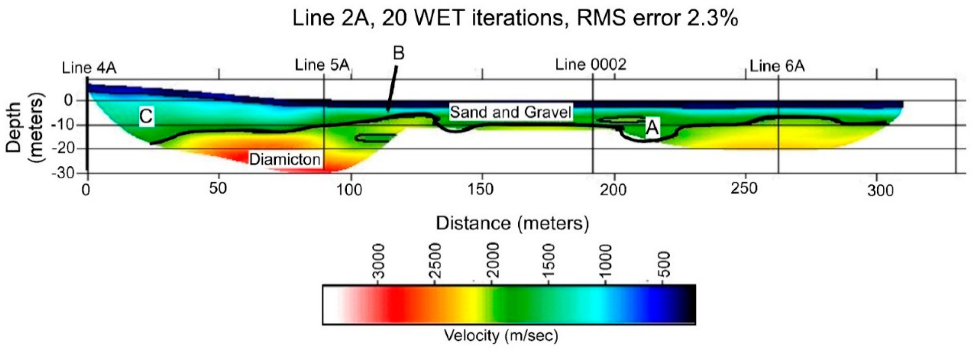
Line 2A (Figure 10) is the north-south profile along the western boundary of the study area. This land surface here displayed the most topographic relief, thus the south (left) end of this profile is ~7 m above the lowermost topographic elevation in the study area. The Cahokia and Henry may be absent at the north end of this line, and the Delavan may be at the surface. This situation would create a velocity anomaly. Along this section, either two distinct channels are evident, or the change in elevation at the south end of the velocity profile has affected depth resolution there. The main channel (A in Figure 10) is about 200 m in width (distance 130–330 m) and is as much as 19 m deep. At about distance 125 m, there is a paleotopographic high at the base of the Henry Formation sand and gravel (B in Figure 11). This could either be a levee between channels A and C, or it could be a velocity anomaly as discussed above. Channel C occurs at the south end of the profile, and is as much as 25 m deep.

Figure 10. North-South velocity profile of Line 2A. South is to the left. Areas A and C are channels, and area B represents a paleotopographic high such as a terrace or is velocity anomaly.

Figure 10. North-South velocity profile of Line 2A. South is to the left. Areas A and C are channels, and area B represents a paleotopographic high such as a terrace or is velocity anomaly.

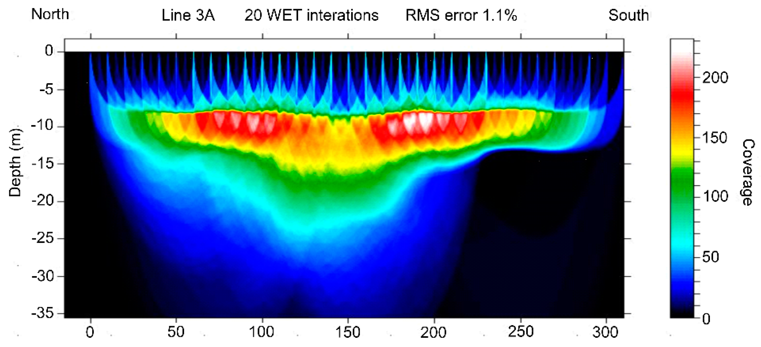
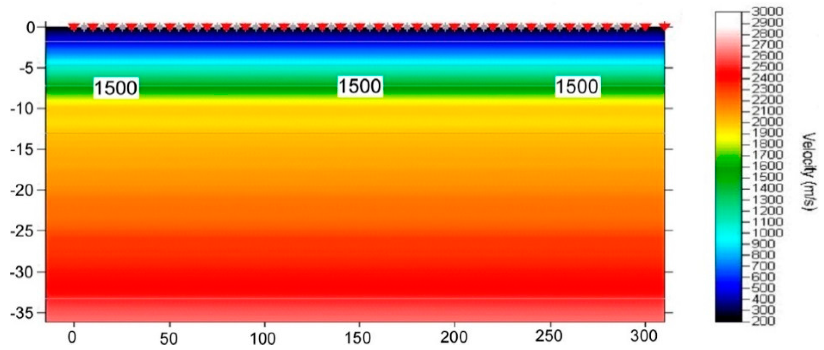
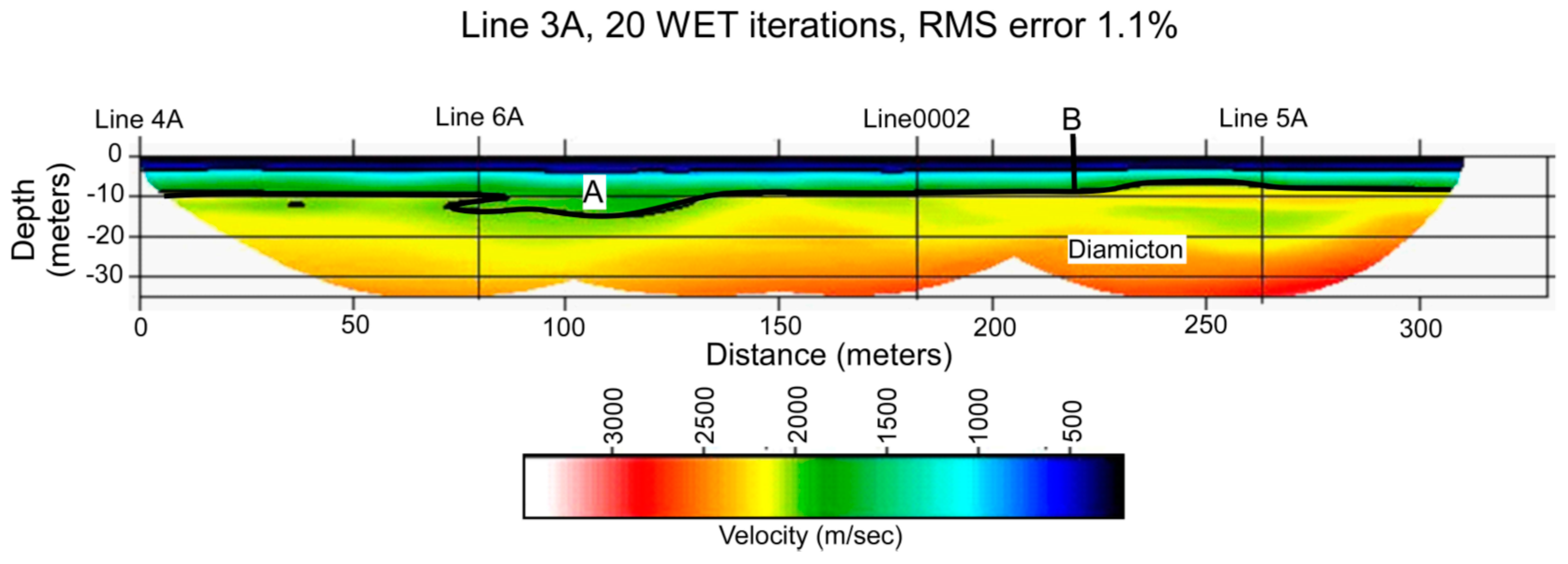
Figure 11. North-South velocity profile of Line 3A with geologic interpretation. South is to the left. A = Channel position; B = terrace elevation.

Figure 11. North-South velocity profile of Line 3A with geologic interpretation. South is to the left. A = Channel position; B = terrace elevation.

Line 3A (Figure 11) is the north-south velocity profile along the eastern boundary of the study area. Only one shallow channel (indicated by A in Figure 11), about 40 m wide and ~5 m deeper than the terrace elevation (indicated by B in Figure 11) is present here.

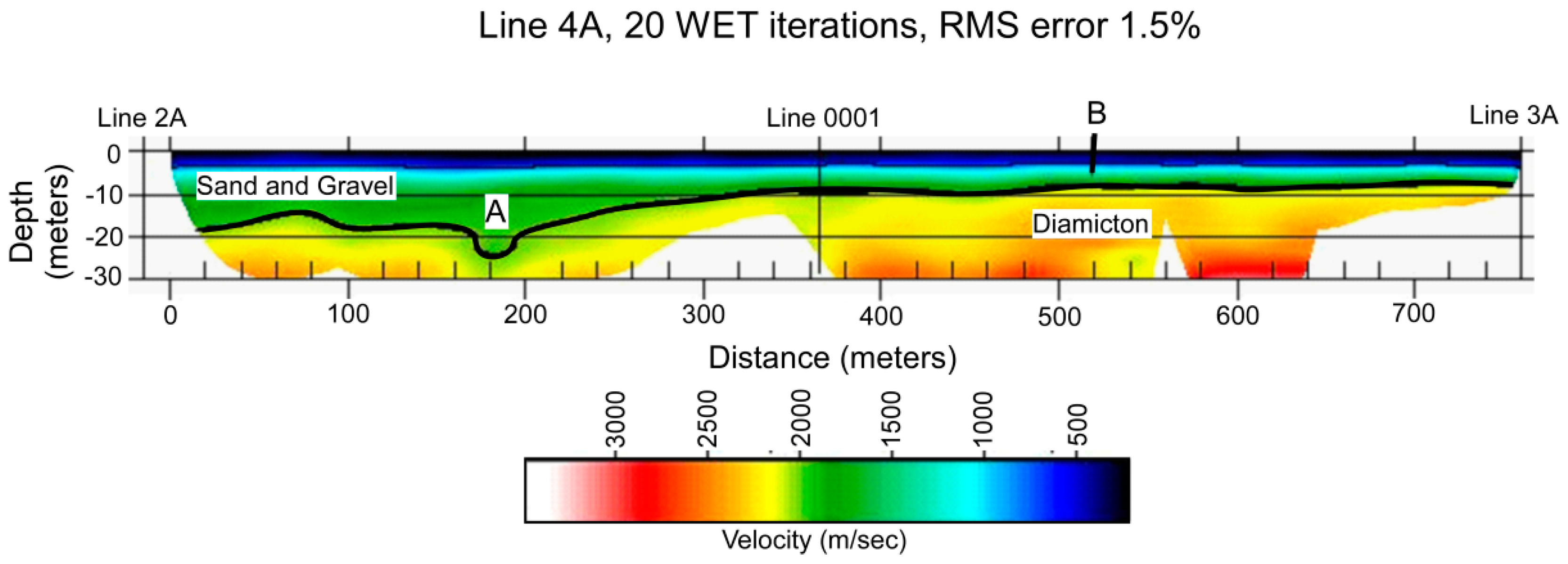
Line 4A (Figure 12) is the east-west trending velocity profile that runs along the southern boundary of the study area. West is to the left. Here the channel (A on Figure 12) is about 300 m wide. The deepest part of the channel is about 185 m from the west end of the profile, is 10 m wide, and reaches a depth of about 22 m. The terrace (B on Figure 12) base is consistently about 10 m in depth and occurs from the intersection of Line 0001 and extends to the east end of the profile.

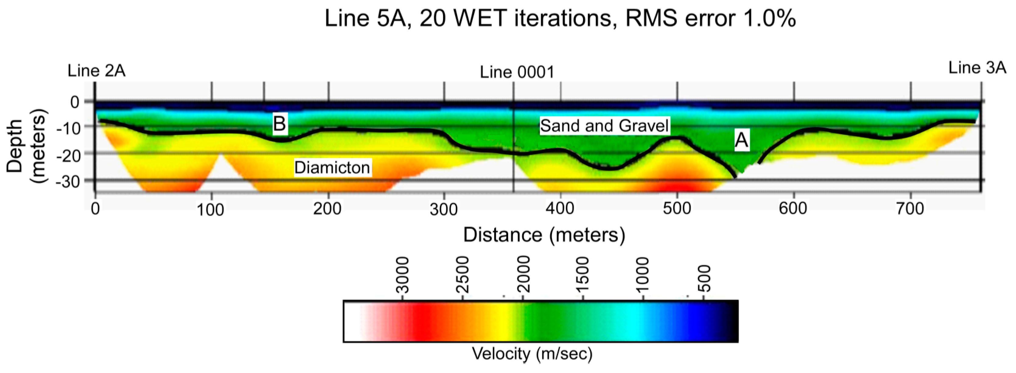
Line 5A (Figure 13) is about 80 m north of and parallel to Line 0002. West is to the left. Here the channel extends from distances 300–600 m and reaches almost 30 m in depth (labeled A in Figure 13) at distance ~550. The terrace surface here is more gently undulating here than it is the other velocity profiles. Some smaller (10–20 m wide at 5 m deep) channels occur on the terrace (e.g., B in Figure 13).

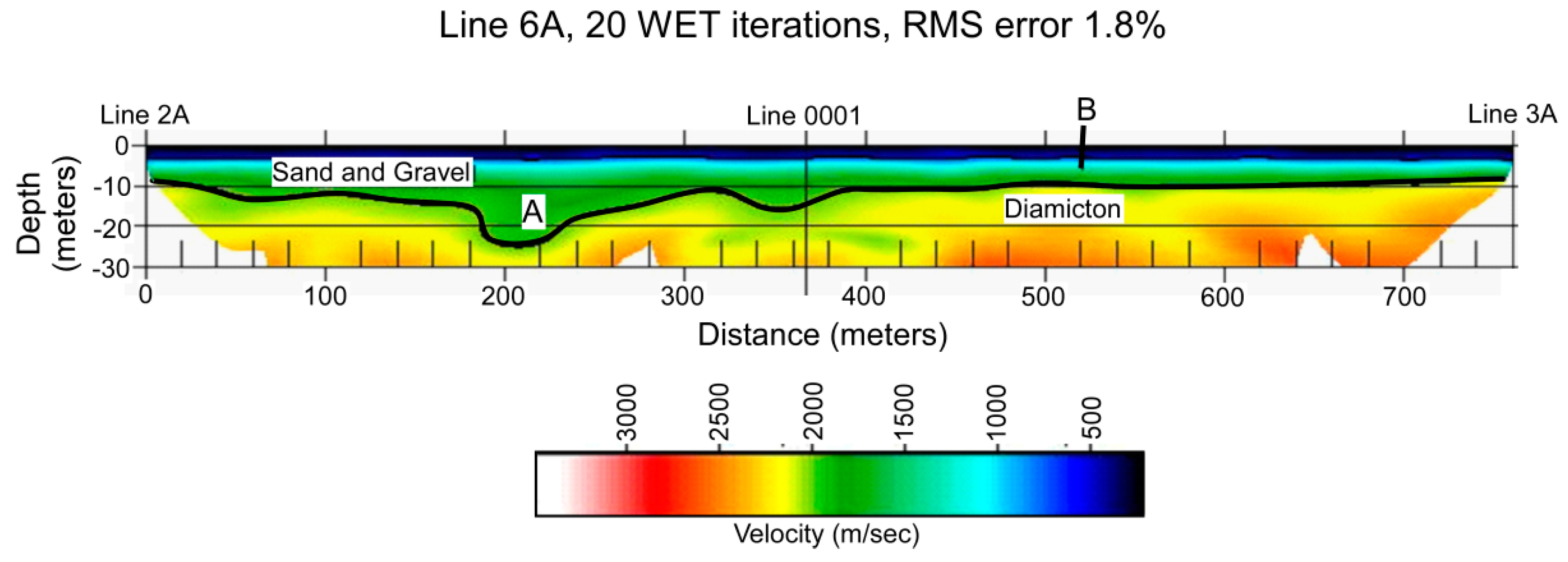
Line 6A (Figure 14) is an east-west profile that was shot about half way between Line 0002 and Line 4A. Along this profile, the channel runs from distance 50 m to 400 m (350 m wide) and is as much as 25 m in depth (indicated by A in Figure 14). As in the other profiles, the base of the terrace (indicated by B in Figure 14) is about 10 m.

Figure 12. Seismic velocity profile of Line 4A, east is to the right. A = deepest part of the channel; B = the terrace elevation.

Figure 12. Seismic velocity profile of Line 4A, east is to the right. A = deepest part of the channel; B = the terrace elevation.

Figure 13. Seismic velocity profile of Line 5A, west is to the left. A = main channel; B = smaller channel on the terrace.

Figure 13. Seismic velocity profile of Line 5A, west is to the left. A = main channel; B = smaller channel on the terrace.

Figure 14. Seismic velocity profile of Line 6A. A = main channel, B = terrace.

Figure 14. Seismic velocity profile of Line 6A. A = main channel, B = terrace.

6. 2-D Velocity Data Conversion

Although Petrel is designed to readily import 2-D and 3-D seismic reflection data, the software is not currently designed to import seismic refraction data. Moreover, Petrel is designed to model the deep rather than shallow subsurface. Thus, the refraction velocity data had to be converted into a format that Petrel can use. This process is outlined below.

Surfer 8 files from the 2-D velocity models can be viewed as grid files in X, Y, Z ASCII format, which allows for multiple modeling software systems to use the SEG-2 data sets. These files were imported into Microsoft Excel to be converted into three dimensions by using a simple point slope formula to calculate the true north/easting every 0.05 meter in the X and Y direction. Z values are represented as depth. Aside from the northwest corner of the study area, the site is flat (± 1 m). Thus, we have made the assumption that the ground surface Z = 0 m. This allows graphical depths to be easily read along the z-axis.Following coordinate conversion and velocity data filtering, each 2-D grid file was imported into Petrel.

7. Petrophysical and Seismic Velocity Modeling

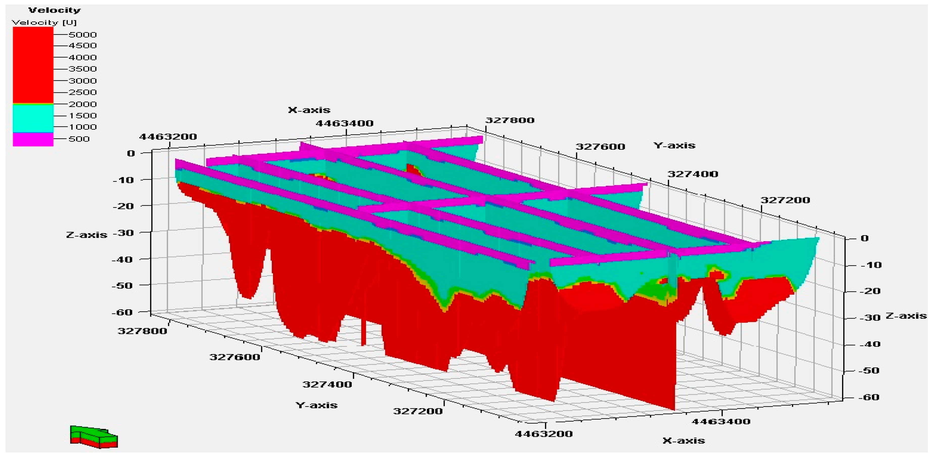
During the creation of the petrophysical model, velocity and depth profiles were upscaled into the 3-D grid through the process of “Scale Up Well Logs”. This process takes a variety of data and incorporates it into the 3-D grid assigning the corresponding grid nodes with the datasets values (Figure 15). Once upscaled, the data was extrapolated throughout the 3-D grid assigning each cell a value using the Convergent Interpolation algorithm. Figure 16 displays the final petrophysical model used to interpret the 3-D geology of the study area.

Figure 15. Upscaled velocity attribute into the 3-D grid. Cells intersecting the upscaled dataset are given the respective value which are then interpolated during petrophysical modeling.

Figure 15. Upscaled velocity attribute into the 3-D grid. Cells intersecting the upscaled dataset are given the respective value which are then interpolated during petrophysical modeling.

Figure 16. Completed petrophysical model of the seismic velocity attribute. All cells within the grid were assigned a value using the convergent interpolation algorithm. West is indicated by the green arrow.

Figure 16. Completed petrophysical model of the seismic velocity attribute. All cells within the grid were assigned a value using the convergent interpolation algorithm. West is indicated by the green arrow.

Using the petrophysically modeled velocity attribute within the 3-D grid, a velocity model was created with the same geometry and resolution as the petrophysical model using Petrel’s “Make a Velocity Model” process. As with the petrophysical model, velocity models were run at 1 m² grid spacing. Convergent Interpolation was chosen as the processing algorithm.

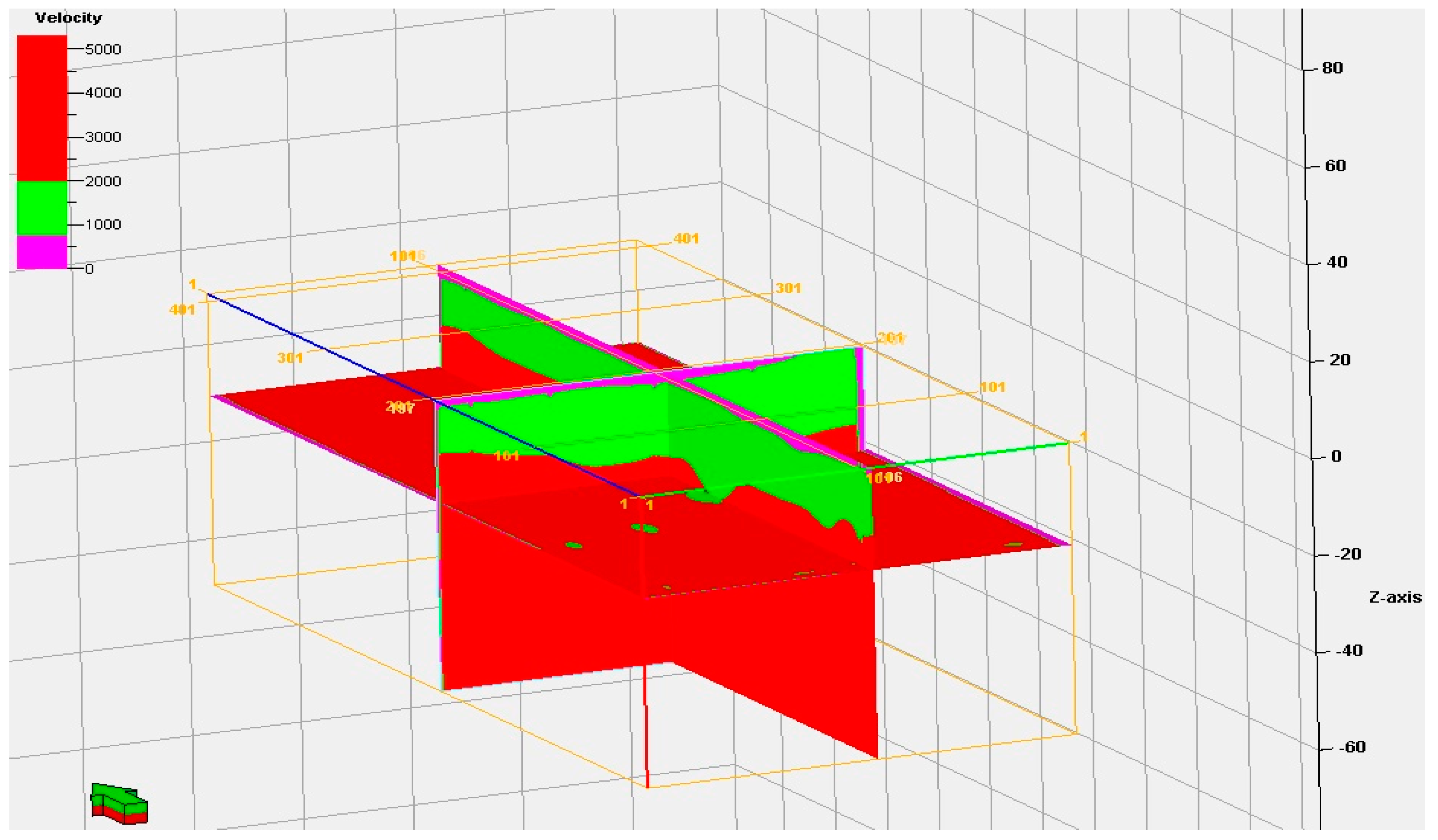
In order to create a velocity model with refraction data processed within Rayfract 3.14, Petrel requires the Z component be converted from depth to time. This conversion needs to take place because the seismic output data from Rayfract 3.14 is represented as depth rather than time. All other parameters were left as default and run with the velocity model tool. The steps to create the velocity model allowed the 2-D refraction data to be converted from depth with associated velocity attribute into an artificial 3-D velocity grid in time. The final velocity model mimics a true 3-D reflection velocity model (Figure 17).

After the synthetic 3-D reflection dataset was generated, the geologic interpretation of the Henry Formation is possible. Seismic interpretation allowed us to manually select/create several point data by moving velocity cross-sections in two dimensions to build a 3-D seismic horizon. These horizons can be used to generate surfaces, point data sets (artificial formation tops), and contacts opening up a wide array of processes and analysis tools. For this project, the purpose of creating a 3-D model is to determine the channel features and geometry (slope, strike, channel features, and depth), as well as the bulk volume of sand and gravels within the subsurface. (Figure 18 and Figure 19).

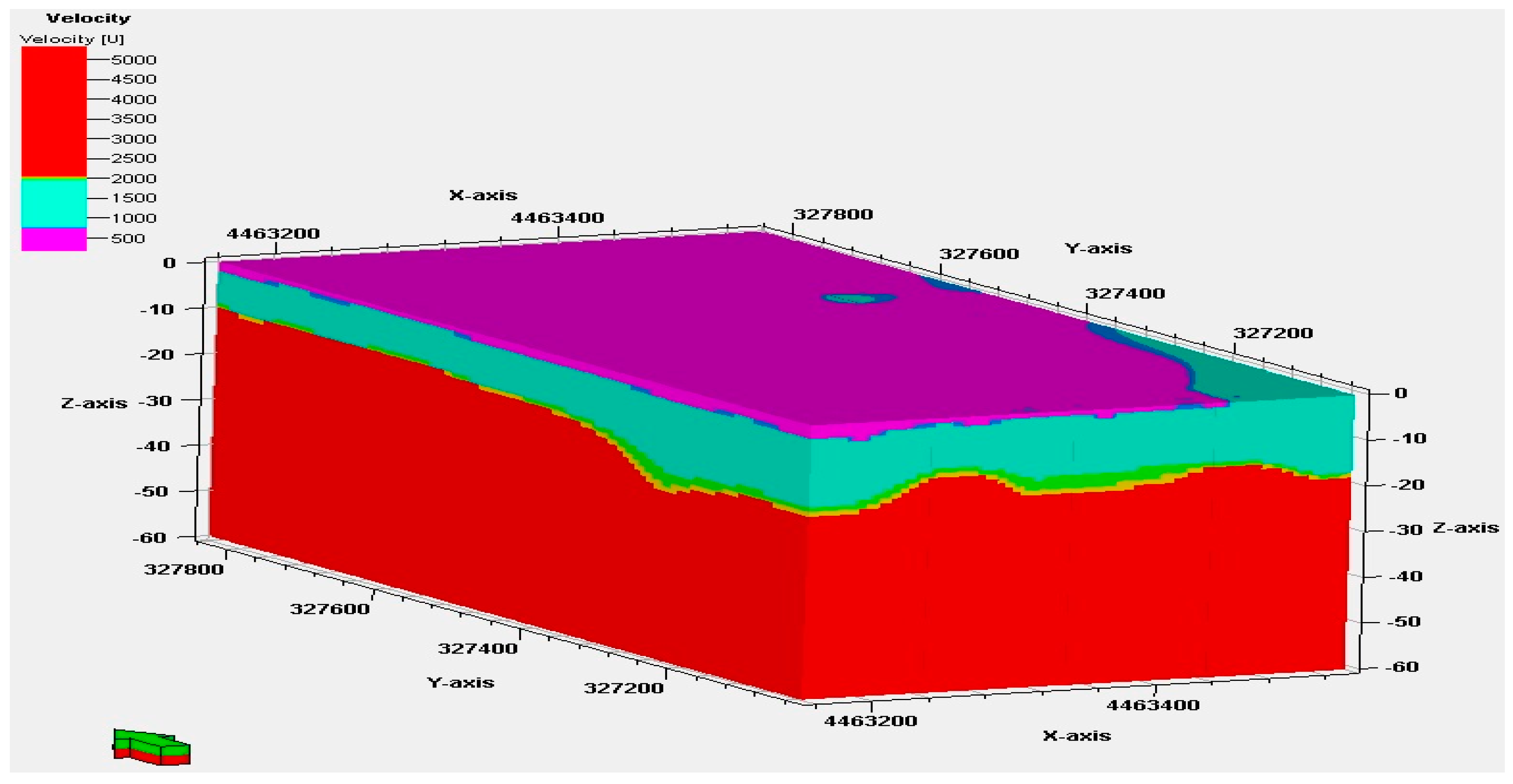
Figure 17. The final velocity model which was used for geologic interpretation. The cross sections are along Line 0001 and Line 0002. The green arrow points to the west. Red indicates till of the Delavan Formation, green is the Henry Formation outwash, and purple is the Cahokia Formation alluvium.

Figure 17. The final velocity model which was used for geologic interpretation. The cross sections are along Line 0001 and Line 0002. The green arrow points to the west. Red indicates till of the Delavan Formation, green is the Henry Formation outwash, and purple is the Cahokia Formation alluvium.

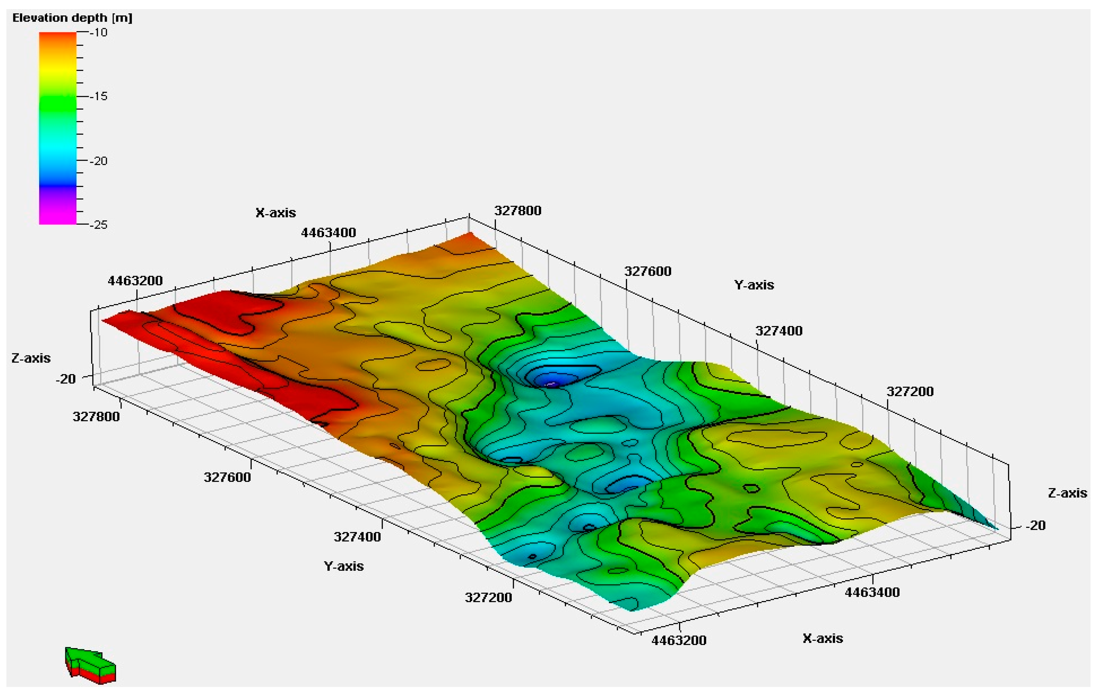
Figure 18. Structure contour map of the top of the Delavan Till. West is to the left. Contour interval = 1 m.

Figure 18. Structure contour map of the top of the Delavan Till. West is to the left. Contour interval = 1 m.

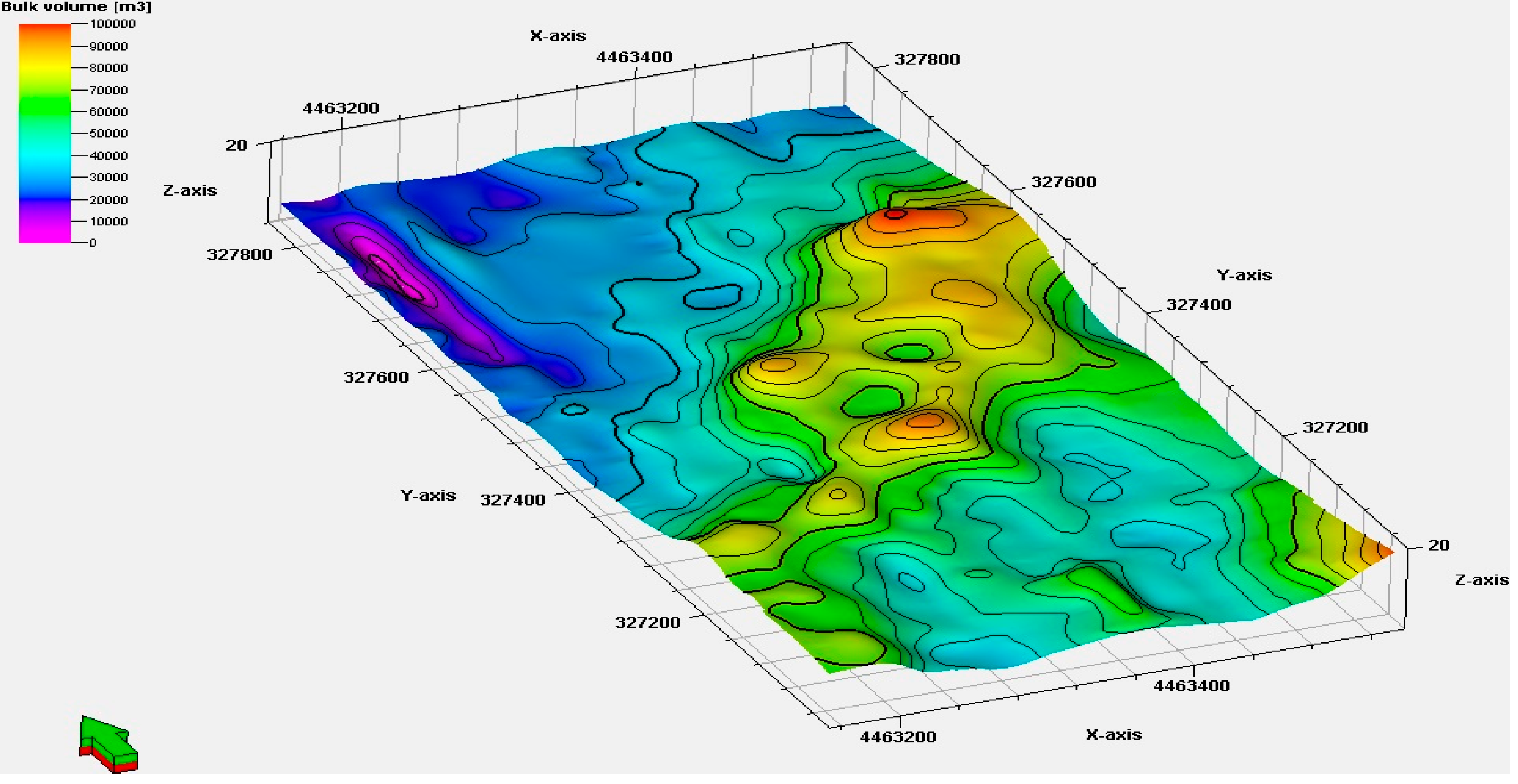
Figure 19. Isopach map of the Henry Formation in the study area that displays the bulk volume of sand and gravel. Vertical exaggeration is 5X.

Figure 19. Isopach map of the Henry Formation in the study area that displays the bulk volume of sand and gravel. Vertical exaggeration is 5X.

8. 3-D Model Results

Figure 18 is a structure contour map constructed on the base of the Henry Formation. The 3-D geological model reveals that, with the exception of the northwest corner, both the Cahokia and Henry formations occur throughout the study area. The Cahokia Formation is a blanket deposit, and is consistently 2–3 m in thickness. The thinnest Henry Formation, which occurs above the terraces in the northeast and southwest regions of the study area. The highest terrace is to the southwest. The deepest part of the channel trends about S15°E, which is oblique to the consistent S55°W trend of the modern Kickapoo Creek valley. Here the Henry Formation is as much as 25 m in thickness. The channel is 100–200 m in width. No significant tributary valleys are evident.

Volumetric calculations were achieved by creating contacts between the basal till and Henry Formation, as well as the Henry Formation and top-soil. These contacts effectively constrain the Henry Formation between to bounding contact surfaces. Because Petrel’s volume calculations deal primarily with fluid (oil, gas, and water), all settings with regards to permeability, porosity, and such were left with the default values; and only bulk volume values were analyzed with this function. Figure 19 displays the bulk volume surface generated by Petrels volumetrics process, this surface was used to highlight the regions with the most abundant amounts of sands and gravels. The output datasheet values are in model units (m³), and must be converted into cubic yards (yd³) to portray relevance within the gravel industry. This conversion was performed by multiplying the Petrel bulk volume output of 4 million m³ by 1.3079. Bulk volume calculations performed in Petrel, yield 4.0 million m³, or 5.2 million yd³ of sand and gravel.

9. Discussion and Conclusions

The Wisconsin Episode glacier retreated from central Illinois beginning about 20,000 years ago and left a series of recessional moraines. Kickapoo Creek, and Sugar Creek 10 km to the northwest (see Figure 2), are parallel and each flow along a nearly linear path toward the S55E, which is normal to the trend of the recessional moraines in this area. These valleys are filled with Henry Formation sand and gravel (i.e., valley train). Each are incised into the Delvan Till, which was deposited during the most recent ice advance. The valley train outwash occurrence is most commonly interpreted a valley being scoured by meltwater and then backfilled by sand and gravel by glacial meltwater away from the terminus of the glacier [13]. Some of these deposits are quite spectacular in their coarseness, and were deposited by torrent release events.

The Henry Formation in the study area consists largely of sand and pebbly sand, with small amounts of gravel interbedded. The most striking aspect of the Henry Formation here is that the trend of the channel at the base of the unit is oblique to the Kickapoo valley by 70°. The most likely explanation for the oblique Henry channel geometry, trend of the Kickapoo valley with respect to the trend of the recessional moraines, and unit texture is that the Henry Formation here was deposited as part of a subglacial tunnel valley rather than traditional valley train. Unlike eskers, which are positive topographic features, tunnel valleys require incision of the underlying sediments before being back-filled.

Tunnel valley have been reported elsewhere in areas affected by the most recent advance of the Laurentide ice sheet. Moores [20] reported on tunnel valleys associated with the Lake Superior Lobe of the Laurentide ice sheet and concluded that ice surface as well as subsurface meltwater contributed to tunnel valley genesis in Minnesota. Similarly, Kehew et al. [21] recognized that subglacial tunnel valleys played an important role in the deglaciation of the Saginaw and Lake Michigan lobes in central Michigan. Cofaig [22] provides an excellent synthesis of tunnel valley description and genesis. He recognized tunnel valleys as elongate troughs that are cut into till, and sometimes bedrock. They are either sinuous or occur as straight valleys and are dominated by sand rather than coarser outwash. He further advocated the tunnels valleys are formed during deglaciation at the ice margin by subglacial meltwater.

In the study area, the Delavan Till was deposited during ice advance. At ice still-stand, glacial meltwater scoured the Delavan Till surface, creating a narrow, deep sub-channel that is oblique to the broader trend of the tunnel valley itself. During ice retreat, the tunnel valley and its sub-channel were filled by large volumes of sand. This sediment was reworked as the ice retreated north of the study area, and the sediment was eventually distributed throughout the Kickapoo Creek valley. A thin blanked of alluvium was deposited during the Holocene erosional cycle.