Wadenow: A Matlab Toolbox for Early Forecasting of the Velocity Trend of a Rainfall-Triggered Landslide by Means of Continuous Wavelet Transform and Deep Learning

Abstract

A procedure aimed at forecasting the velocity trend of a landslide for a period of some hours to one or two days is proposed here together with its MATLAB implementation. The method is based on continuous wavelet transform (CWT) and convolutional neural network (CNN) applied to rainfall and velocity time series provided by a real-time monitoring system. It is aimed at recognizing the conditions that induce a strong increase, or even a significant decrease, in the average velocity of the unstable slope. For each evaluation time, the rainfall and velocity scalograms related to the previous days (e.g., two weeks) are computed by means of CWT. A CNN recognizes the velocity trend defined in the training stage corresponds to these scalograms. In this way, forecasts about the start, persistence, and end of a critical event can be provided to the decision makers. An application of the toolbox to a landslide (Perarolo di Cadore landslide, Eastern Alps, Italy) is also briefly described to show how the parameters can be chosen in a real case and the corresponding performance.

1. Introduction

Reliable forecasts of the velocity trend of a landslide for the next hours/days are very important if such a phenomenon threatens build-up areas or infrastructures. Besides the data provided by a monitoring system, the identification of the triggering factors is necessary for obtaining these forecasts. The most common natural landslide triggers are intense rainfall, rapid snowmelt, water-level change, volcanic eruption, and earthquake shaking [1]. Where persistent and/or intense rainfall triggers the slope motion, the forecasting of landslide behavior is often based on rainfall thresholds [2]. Although these thresholds are widely used to provide regional-scale forecasts, their use for slope-scale forecasts is limited because the rainfall is a measured value possibly correlated with landslide motion but is not a direct measure of it. Nowadays, many advanced remote sensing technologies, from spaceborne sensors, such as very high-resolution optical imagery and Synthetic Aperture Radar (SAR), to aerial and terrestrial sensors, such as laser scanning, photogrammetry, infrared thermography, and ground-based SAR, can provide data about landslide velocity suitable for early warning purposes [3].

Long time series related to both rainfall data and landslide kinematics can be used to evaluate forecasts of slope instability at a time scale of hours and days, under the condition that data are processed by means of advanced methods [4], e.g., machine learning techniques [5].

The continuous wavelet transform (CWT) can provide accurate time localization for high-frequency short events and accurate frequency localization for low-frequency long events, a fact which is very important for applications in geosciences [6]. Since significant landslide accelerations are often due to both very intense short-duration rainfall episodes and long-duration periods of modest or minor rainfall, the CWT can characterize time series related to unstable slopes. For example, seasonal variations of a landslide from interferometric SAR kinematic data and rainfall data by means of CWT can be analyzed [7].

A convolutional neural network (CNN) is a deep neural network characterized by the use of convolution in place of general matrix multiplication in at least one of its layers [8]. The CNNs are currently used in image classification, medical image analysis, natural language processing, and analysis of financial or meteorological time series. CNNs can also be used to automatically recognize landslides and mass movements in images taken from both ground and aerial platforms [9]. Since the training from scratch with random initialization of a CNN requires the availability of a very large number of images (at least tens of thousands), which is unattainable in many applications, and a very long training time, transfer learning is generally carried out [10]. This approach allows the repurposing of an available CNN according to the new needs after the change of the classification layer, with great savings in computing power, computation time, and the amount of required input data. Among the available pre-trained models there are, e.g., the VGG16 and VGG19 CNNs [11]. Deep learning methods, and in particular CNNs, are increasingly used in geohazards assessment [12] and forecasting [13].

The combined use of CWT and deep learning techniques is a recent advance in landslide displacement forecasting. For example, a CWT can be used to decompose the time series of rainfall, reservoir level, and landslide displacement into seasonal and residual components, and the resulting data can be used to obtain forecasts by means of a deep belief network [14]. Velocities are often decomposed into periodic and trend components [15]. In the present paper, another approach is followed. It is based on the use of CNNs in automated analysis and classification of scalograms provided by CWT, which is used in, e.g., automatic detection of atrial fibrillation [16], supporting brain-computer interface for rehabilitation purposes [17], and, in general, time series forecasting [18]. This approach, which does not require signal decomposition, is compatible with transfer learning and, therefore, is characterized by a reasonable computational cost. The proposed procedure is aimed at providing up to 2 days’ forecasts of landslide kinematics by means of CNN-based recognition of the kinematic trend at a given time on the basis of an image provided by CWT, which represents the rainfall and velocity time series related to some previous days (e.g., 15 d).

2. Methodology

The proposed method is based on the following two assumptions: The kinematics of the studied landslide is rainfall-driven, and it is possible to divide the unstable slope into some areas, each having relatively homogeneous kinematics. The described procedure should be applied to each area, with the training of a specific CNN. This means that a specific forecast will be provided for each of these areas and that, therefore, the spatial resolution obtainable with this system depends on their size as well as on the characteristics of the monitoring system that provides the velocity data.

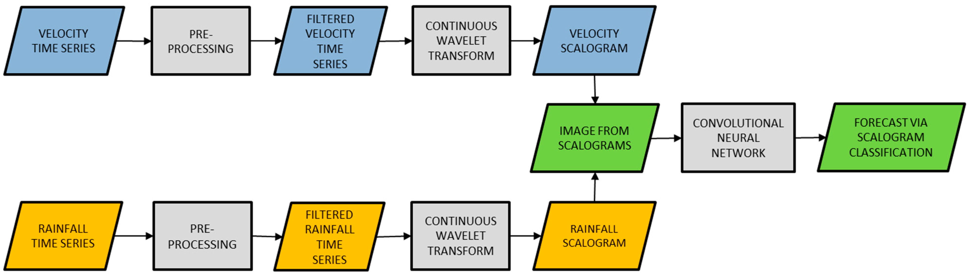
In brief, the proposed method is based on the following (Figure 1):

(1)

Use of CWT in order to provide scalograms of velocity and rainfall time series. Each scalogram is the visual representation of CWT of the corresponding time series and, therefore, for each time interval having a suitable length (depending on the specific monitored slope), an image is generated using the couple of scalograms;

(2)

The scalogram-based image is sent to a specifically trained CNN. This CNN classifies the image and, therefore, recognizes the velocity trend correlated to the corresponding scalograms, leading to a forecasting of the kinematic behavior of the monitored area of the landslide.

The key to the proposed procedure is the CNN-based correlation between the scalograms of rainfall and velocity time series up until a time $t_c$ and the corresponding velocity trend before and after $t_c$. In this way, as the CNN training is completed, the system can provide velocity forecasts in the sense that it indicates what is the expected trend at $t_c$ on the basis of rainfall and velocity time series until up $t_c$. For this reason, the elements to take into consideration are scalogram generation, the definition of velocity trends, and CNN training/operation.

In order to obtain valid scalograms, raw data are pre-processed before the application of CWT. In particular, noise reduction and outlier removal are necessary. The filtering for noise reduction can be carried out, e.g., by means of moving average smoothing or also discrete wavelet transform. Furthermore, in the case of velocity time series, a spatial average may be required within a relatively homogeneous kinematic area, to provide a representative value.

2.1. Scalogram Generation

Some concepts in CWT are briefly summarized here (see e.g., [19] for more information). The CWT of a time series $x\left(t\right)$ is a measure of its similarity with an analyzing function ${\psi }_{a,b}\left(t\right)$, called daughter wavelet, such as follows:

$${\psi }_{a,b}=\frac{1}{\sqrt{a}}\psi \left(\frac{t-b}{a}\right)$$

(1)

where $\psi \left(t\right)$, the mother wavelet, is a zero-average oscillating function well localized both in time and frequency. As $a\ne 0$ (scale factor) and b (translation in time) change, a time-frequency representation of $x\left(t\right)$ is obtained because $f\propto 1/a$, where f is the frequency.

The choice of the mother wavelet is carried out on the basis of the specific application. The Morlet wavelet is an oscillation with a fixed frequency $f_0$ tapered by a Gaussian window with standard deviation (SD) ${\sigma }_t$. It is particularly suitable for detection and analysis of transient signals and, therefore, is largely used as mother wavelet for CWT of geophysical time series [20].

The scalogram of a time series is the absolute value of its CWT, plotted as a function of time and frequency. Since a scalogram can characterize slowly varying signals punctuated by abrupt transients, allowing good time localization of short-duration, high-frequency events and good frequency localization of low-frequency components, it is particularly suitable for analyzing real-world signals. The scalogram is the equivalent for the CWT of what the spectrogram is for the FT.

A scalogram can be affected by edge effects, which occur where the stretched wavelets extend beyond the edges of the observation interval [21]. Several methods aimed at reducing the edge effects are available. They are based either on the signal modification at the edge region, e.g., zero padding, value padding, decay padding, signal repeating, signal reflecting, and also adaptive-wavelet-function methods [22].

The range of the time shift b directly comes from the length of the time series. Let $t_c$ be a time at which the data are analyzed, and a forecast should be provided, expressed in days. For a rainfall time series, the time spans from $t_c-N_A$ to $t_c+N_B$, where $N_A$ and $N_B$ are expressed in days. The value $N_A$ comes from the results of a preliminary comparative analysis of the rainfall and velocity time series. It must be sufficiently large to account for the effects of rainy periods of several days. It should also be taken into account that the images treated with CNN are limited in size (see the Section 2.3). A too-large $N_A$ would affect the effective temporal resolution of the CWT-based analysis. As for $N_B$, if no rainfall forecasts are available, $N_B=0$ must be chosen. If reliable quantitative rainfall forecasts for $N_{RF}$ days are available (typically, $N_{RF}$ is 1 to 2 days), a value $N_B$ such that $0<N_B\le N_{RF}$ could be chosen. If $N_B>0$, this can contribute to reducing edge-effects. Clearly, the corresponding velocity-time series spans from $t_c-N_A$ to $t_c$.

The range of the scale factor $a=f^{-1}$ comes from the specific wavelet and from the Nyquist frequency $f_N=f_S/2$, where $f_S$ is the sampling frequency expressed in cycles per day (cpd).

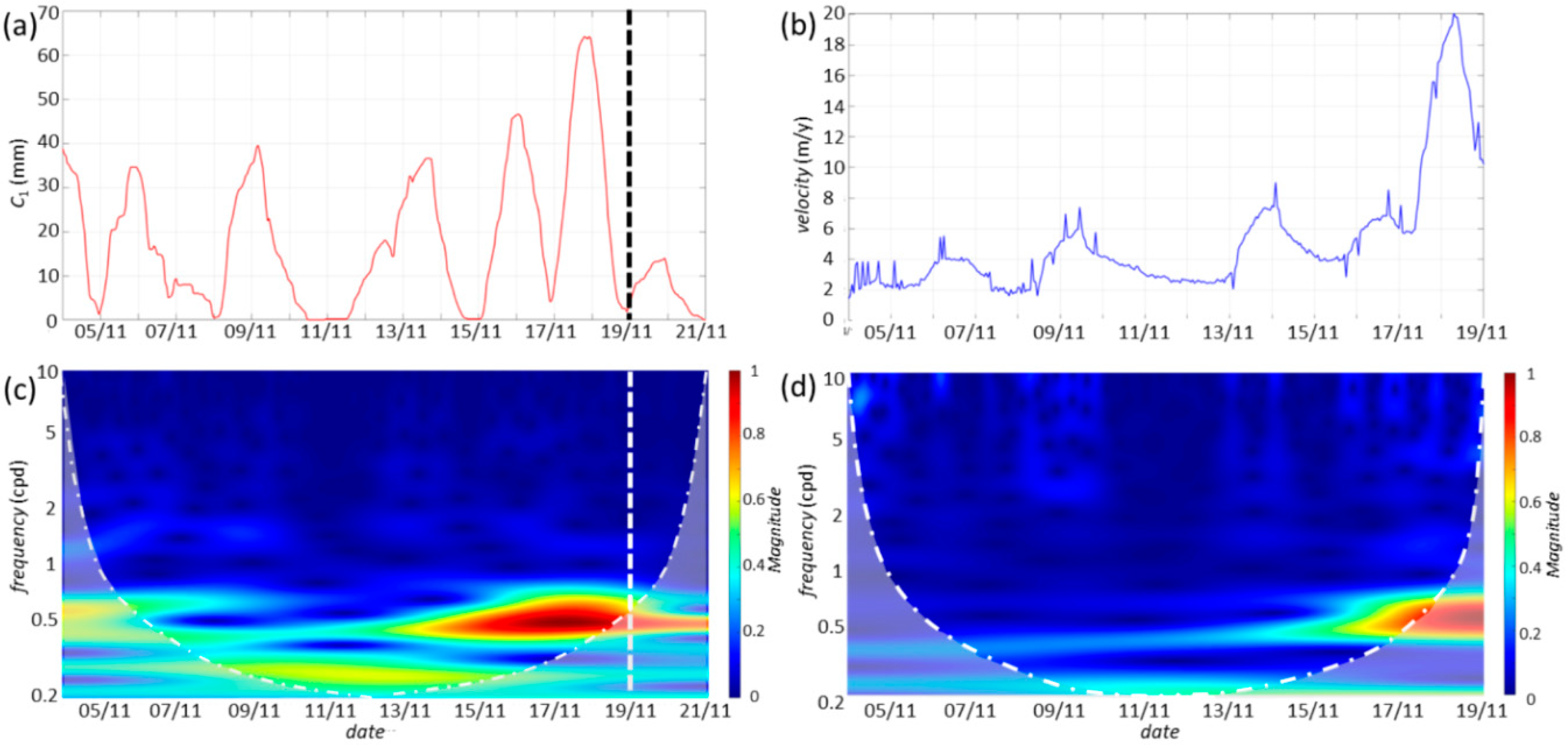
Examples of rainfall and velocity time series and corresponding scalograms are shown in Figure 2, where $f_S=24 \mathrm{cpd}$ ($f_N=12 \mathrm{cpd}$). They are related to an extreme phenomenon occurred in November 2019 at Perarolo di Cadore (see Section 4 for more information). The Cones of Influence (COIs), i.e., the scalogram regions where edge-effects become important, are computed according to [6]. In this case, the edge-effects are completely negligible for $f\ge 1 \mathrm{cpd}$. In case of rainfall, even if only moderately intense, peaks are observed in this frequency band. For frequencies in the range 0.5−1 cpd, where important scalogram peaks are observed, the edge-effects are reasonably low (Figure 2c,d) and disappear in the velocity scalogram if $N_B=2 \mathrm{d}$ is chosen. The lower frequency range, where the edge-effects are higher, has less importance. The scalograms shown in Figure 2 are computed with the default parameters used for the Morlet wavelet in MATLAB, i.e., ${\omega }_0=2\pi \omega f_0=6{ \mathrm{d}}^{-1}$ and ${\sigma }_t=1 \mathrm{d}$. These parameters are suitable for large part of applications.

2.2. Velocity Trends

The velocity trend at a time represents the kinematic state of the landslide (or of a portion of the landslide if more than one kinematic area is recognized) at that time. It comes from the velocity time series from $t_c-N_C$ to $t_c+N_D$, where $N_C$ and $N_D$ are chosen on the basis of the typical response with time to rainfall stimuli of the specific landslide. Clearly, it should be $N_A\ge N_C$. In the training stage, the CNN learns to correlate the scalograms of rainfall and velocity with the velocity trends. In the operation stage, the CNN can determine the expected velocity trend from input scalograms and, therefore, can provide trend forecasts.

Let $v_S\left(t\right)$ be the velocity provided by the monitoring system at the time t. The landslide velocity is assumed to be low, mid, or high if $v_S\left(t\right)\le V_M$, $V_M<v_S\left(t\right)\le V_H$ or $v_S\left(t\right)>V_H$ respectively, where the thresholds $V_M$ and $V_H$ are chosen on the basis of the behavior of the unstable slope and, if available, the results of numerical modeling. These thresholds can be constant- or time-dependent. The mentioned terms low/mid/high velocity are related to different kinematic conditions of the specific landslide or portion of a landslide. In particular, these terms are not related to the Varnes’ 1978 landslide classification system [23]. Moreover, in order to avoid or at least reduce wrong or improper labeling due to spikes, the corresponding MATLAB function recognizes a threshold as exceeded if there are at least 5 exceedances (this number can be customized). As the thresholds are defined, the velocity trends for CNN training can be labeled in a completely automatic way.

The following seven possible trend labels can be considered:

• L₁: low velocity;
• L₂: transition from low to mid velocity and emission of a pre-alarm signal;
• L₃: mid velocity;
• L₄: transition from mid to high/extreme or from low to high/extreme velocity and emission of an alarm signal;
• L₅: high (or extreme) velocity;
• L₆: transition from high/extreme to mid velocity and possible non-automatic emission of an alarm reset signal;
• L₇: transition mid/low velocity and possible non-automatic emission of a pre-alarm reset signal.

2.3. CNN Training and Operation

A CNN consists of a convolutional base, aimed at generating some features from the input image and composed by a stack of convolutional and pooling layers, and a classifier, aimed at classifying the image on the basis of the features detected by the convolutional base and usually composed by fully connected layers. The transfer learning is carried out by replacing the original classifier with a new classifier that fits the new classification purposes and using suitable input data for CNN training. In this way, the pre-trained model is repurposed in accordance with the new requirements.

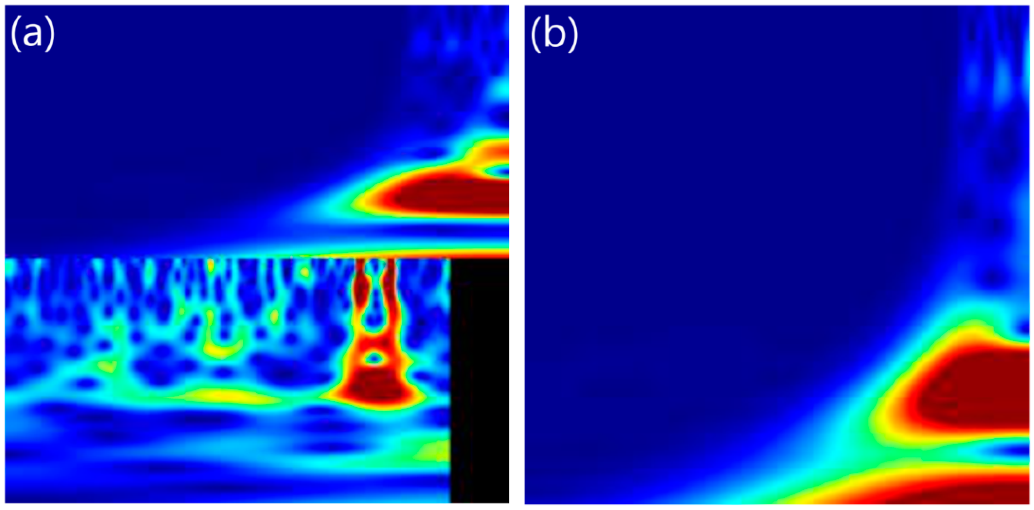
In this case, the input images for the CNN training and operation represent scalograms and the outputs describe the corresponding velocity trends. Each image shows two scalograms (Figure 3a). If $N_B>0$, the alignment of the scalograms is kept by means of zero-padding of the velocity one.

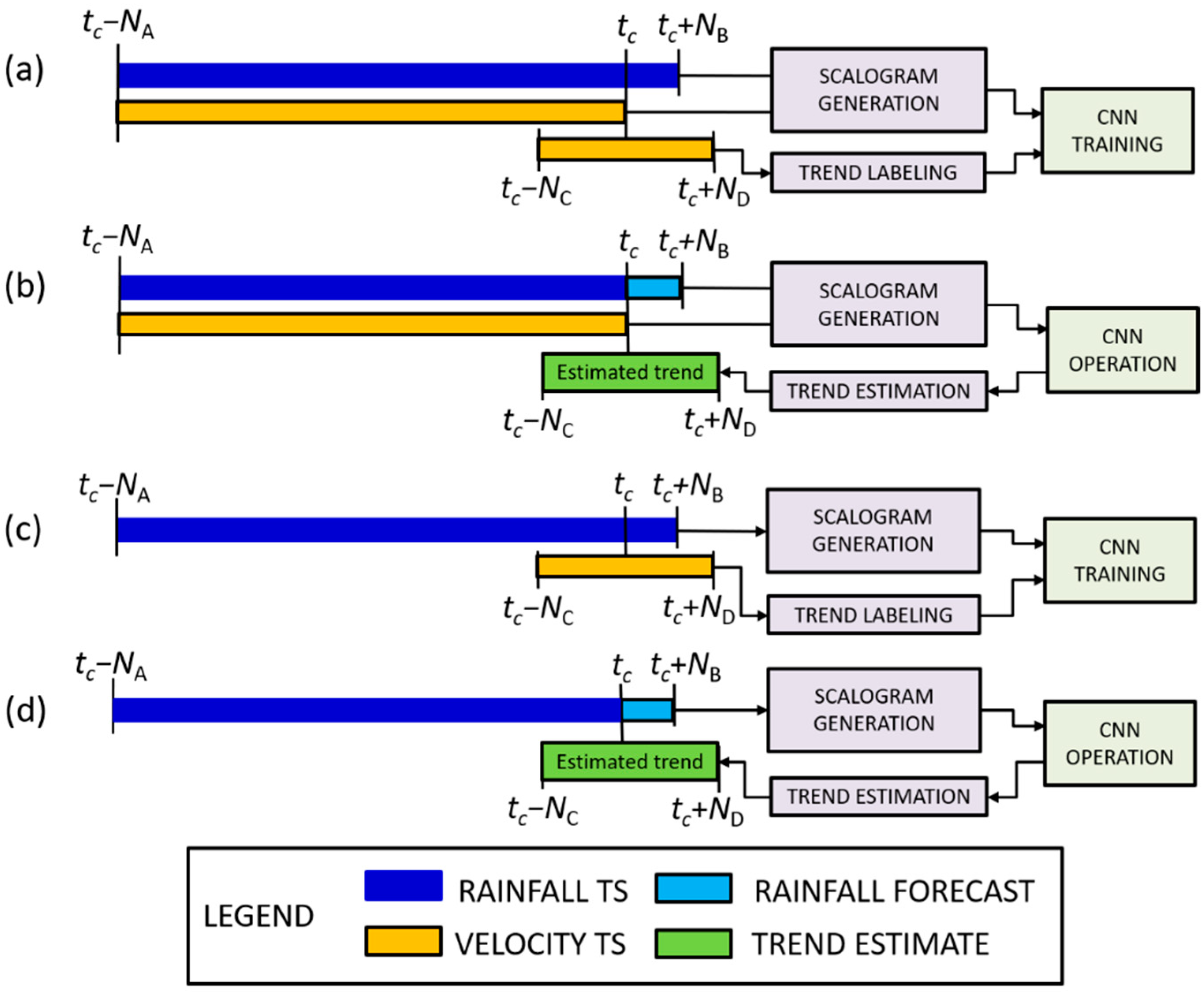
In the training stage the velocity data are used for both scalogram computation and trend labeling. If $t_c$ is a generic training time, the input rainfall time series spans from $t_c-N_A$ to $t_c+N_B$, whereas the input velocity time series spans from $t_c-N_A$ to $t_c$ (Figure 4a). The velocity trend in the interval from $t_c-N_C$ to $t_c+N_D$ is labeled as described in the previous section and is used as a known output of the CNN.

In the forecasting modality (Figure 4b), both the rainfall and velocity time series provided by the monitoring system span from $t_c-N_A$ to $t_c$ (here $t_c$ is the generic operation time), whereas the rainfall data from $t_c$ to $t_c+N_B$ are taken from the weather forecasts. The velocity trend, which is the kinematic forecast in such a modality, is provided by the CNN.

The CNN should provide particularly reliable predictions in the L₄ case because a missed alarm can cause immediate problems, also considering that false alarms should be avoided. If an extreme event occurs, a sequence of CNN outputs could be L₁ → L₂ → L₃ → L₄ → L₅ → L₆ → L₃ → L₇ → L₁, where the segment L₂ → L₃ → L₄ might take place in a few hours and the segment L₆ → L₃ → L₇ → L₁ (i.e., the recovery of pre-crisis velocity) might require several days or several weeks. If the event is very brief, L5 could be lacking. Direct transitions could also occur, e.g., L₁ → L₃ → L₄, or also L₁ → L₄.

In order to provide forecasts when the monitoring system is temporarily out of order or off-line, another CNN is trained with images showing rainfall scalograms only (Figure 3b and Figure 4c,d).

In order to carry out good training, the seven sets of input data should have a roughly equal size. Nevertheless, it is reasonable to expect that the L₁ cases are numerically prevalent over the others, and the extreme cases are probably few. For this reason, data augmentation, which is aimed at artificially creating new training data from existing ones, could be required to have enough trends in L₄ and L₆. According to [24], data augmentation is carried out by adding noise to the time series related to L₄, L₅, and L₆ trends in order to have slightly varied scalograms and, therefore, varied input images. Since data augmentation adds variance without losing the information carried by the data, this allows both the reduction of the risk of overfitting and the improvement of the CNN accuracy on unseen data.

Finally, the data of each set L₁-L₇ are randomly subdivided into three subsets, e.g., 60% for the training, 20% for the validation, and 20% for the test. The training data are actually used to train the CNN, namely, the model sees and learns from these data. The validation data are used in the training stage to evaluate the model’s skills while it is tuned. The model occasionally sees the validation data but does not learn from them. Finally, the test data are used to provide an unbiased evaluation of the performance of the trained CNN. If the test is passed, i.e., at least the critical outputs L₄, L₅, and L₆ are correctly recognized, the CNN can be used in normal operation to provide forecasts.

2.4. Some Details on WADENOW Toolbox

The MATLAB implementation is the set of scripts and functions called WADENOW (WAvelet- and DEep learning-based NOWcasting of landslide kinematics). MATLAB 2018a, or later releases, the MATLAB Wavelet and Deep Learning Toolboxes, and at least one of the MATLAB support packages AlexNet, VGG16, VGG19, GoogLeNet, and ResNet-18 are required (please note that some of these support packages are only available with MATLAB releases newer than 2018a). At least 4 GB of RAM are required (16 Gb recommended). Moreover, a graphical processing unit (GPU) equipped with NVIDIA CUDA^® Toolkit is strongly recommended in order to accelerate the computations in the training stage.

A structure array defined at the beginning of the calculation process allows the definition of all the main options, in particular the type of wavelet and all the necessary parameters. This array is called, similar to an object, by all the WADENOW components. The user can choose between the default wavelet (analytic Morlet with ${\omega }_0=2\pi \omega f_0=6{ \mathrm{d}}^{-1}$ and ${\sigma }_t=1 \mathrm{d}$) and a generic analytic Morlet wavelet. In order to allow this choice, the scripts provided by [25], which are modified versions of the ones in [6], are added to WADENOW. Since the Erickson’s scripts allow the choice of ${\omega }_0$ only, further modifications were carried out in accordance with [19] to allow the choice of ${\sigma }_t$.

The following steps are implemented:

• Rainfall and velocity time series inspection and pre-processing aimed at the following: removing possible spikes, reducing the noise and computing a spatial averaged velocity value for each kinematic area;
• Scalogram computation and image generation. The input image size must be compatible with the used CNN model, e.g., square color images with 224 pixels in the case of VGG19;
• Trend labeling on the basis of chosen thresholds;
• Data augmentation to obtain balanced datasets;
• Partition of scalogram images into training, validation and test datasets;
• Transfer learning of a pre-trained CNN model, or training resume;
• Operation aimed at forecasting the velocity trends from monitoring data at the hours defined by means of a Task Scheduler in the specific Operating System.

The proposed toolbox is completed with some functions for the processing of rainfall and monitoring data to obtain time series with the necessary properties. The WADENOW user’s guide describes in detail all the developed code, which is completely available to the user and can be freely downloaded from the site shown in the Data Availability Statement of this paper.

3. Results in a Real Case

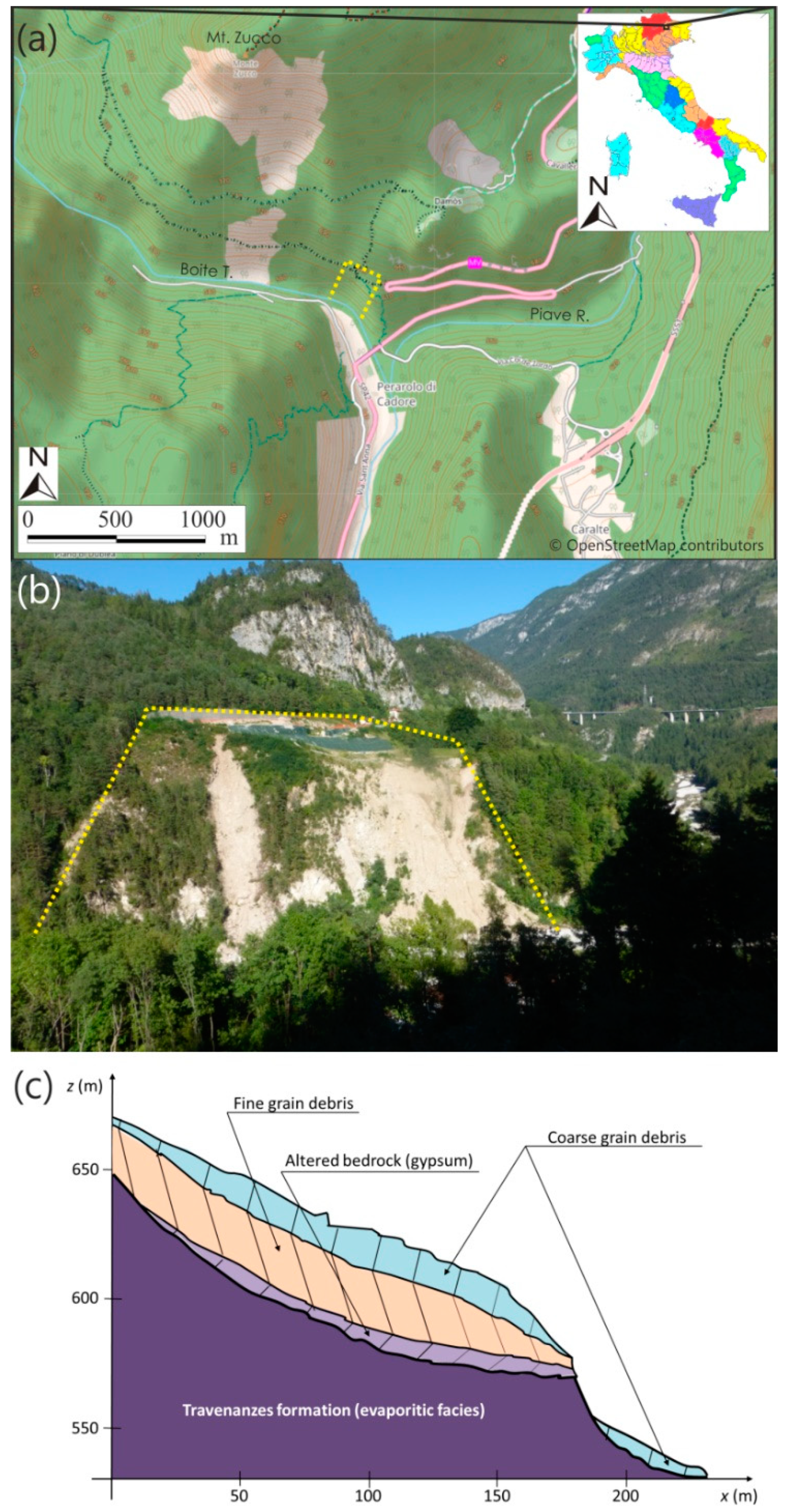
In order to show how the toolbox works in a real case, it was applied to the Sant’Andrea landslide of Perarolo di Cadore (Belluno Province, Veneto Region, Italy), here simply called the Perarolo landslide.

3.1. Geological Setting

The Perarolo landslide is a complex landslide that involves the lower part of the southern slope of Mt. Zucco, just upstream from the confluence between the Boite Torrent and the Piave River [26,27,28], Figure 5a. This landslide is the down-slope part of an old, much greater landslide that affected the entire slope over a height of many hundred meters. Since its collapse could form a temporary dam on the underlying Boite Torrent, directly threatening the nearby village of Perarolo, the induced risk is fairly high. Some stabilization works were carried out on the upper part of the unstable slope in 2001, 2009, and 2018 (Figure 5b), but no effective long-term slope stability effects were reached.

The local stratigraphy (Figure 5c) is composed of a shallow portion of loose debris, characterized by heterogeneous coarse materials mixed with a silty-clay fraction, which is overlapped by a second debris layer, constituted by a predominant clayey-silty matrix with intercalations of anhydrite and heterogeneous detrital sandy-gravelly-silty material. At the base of the loose soils, there is a 5–20 m thick layer of altered anhydrite and gypsum and, below, a stiffer bedrock whose lithological sequence consists of evaporitic facies related to the Travenanzes Formation [29]. The results of electrical tomography and piezometric measurements allowed the recognition of the following two aquifers: a shallow one, affecting the covering detrital layer and supported by the clayey-silty soil, and a deep one, affecting the fractured gypsum.

Numerical modeling helped in estimating the volume of the material that would be mobilized in the case of slope collapse, i.e., $~6\times {10}^4 {\mathrm{m}}^3$, as well as in evaluating the possible post-collapse evolution [27].

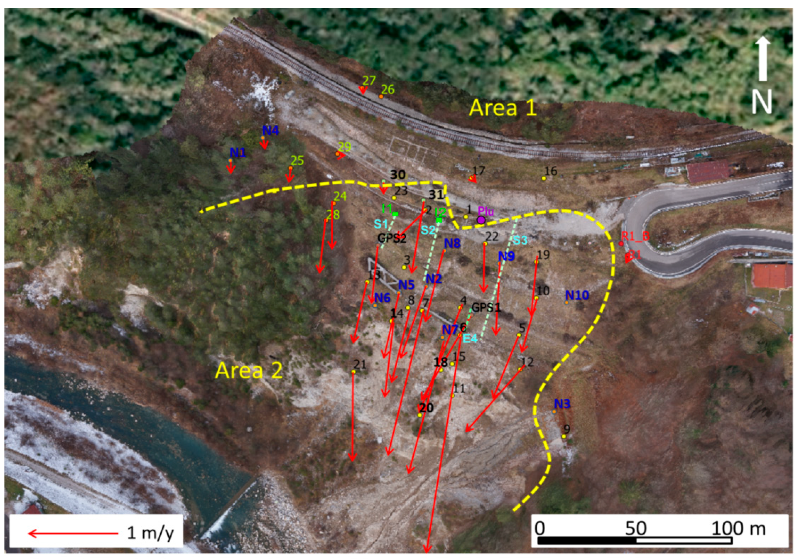
3.2. Landslide Kinematics

Since November 2012, a robotized total station (RTS) has acquired at scheduled times the positions of 50 corner cube reflectors, 45 of which are distributed on the unstable slope and 5 in neighboring areas for reference purposes. The data show that the following two kinematic areas can be recognized in the unstable slope (Figure 6 and

Table 1. Main data about kinematics of Perarolo landslide for each recognized area: low velocity (i.e., mean velocity without rainfall triggering); peak velocity, fraction of episodes where the velocity exceeds three times the corresponding velocity standard deviation ($f_{3\sigma }$), mean velocity in the complete time span.

Time Span	Area 1				Area 2
	Low (m/y)	Peak (m/y)	${\mathit{f}}_{3\mathit{\sigma }}(\%)$	Mean (m/y)	Low (m/y)	Peak (m/y)	${\mathit{f}}_{3\mathit{\sigma }}(\%)$	Mean (m/y)
December 2002–July 2005 1	-	-	-	~0	-	-	-	0.15
June 2006–December 2009 2	-	-	-	-	0.12	1.0	6.6	0.16
January 2010–November 2013 2	-	-	-	-	0.18	1.9	3.5	0.23
November 2013–December 2016 3	0.032	1.6	1.2	0.048	0.38	17	5.2	0.54
January 2017–December 2018 3	0.023	0.8	3	0.038	0.43	30	8.1	0.61
January 2019–December 2019 3	0.016	2.2	2	0.042	0.55	20	4	0.80
January 2020–December 2020 3	0.015	1.8	1	0.026	0.70	20	10	1.3

¹ Data from TLS measurements and, therefore, only related to mean velocities (from [26]). ² Data from two GNSS receivers placed in Area 2; no data about Area 1 are available. ³ Data from robotic total station.

):

• Area 1, with mean velocity of ~3–5 cm/y, where y indicates the non-SI unit year, relatively constant in all the monitored period. The reflectors in this area are observed every 4 h;
• Area 2, with higher velocity, also gradually increasing with the time, from (~0.15 m/y in 2003–2005 to ~1.30 m/y in 2020). The reflectors in this area are observed once per hour.

A pluviometer placed on the landslide crown provides data four times per hour. Rainfall time series with $f_S=24 \mathrm{cpd}$ were obtained by taking hourly cumulative values.

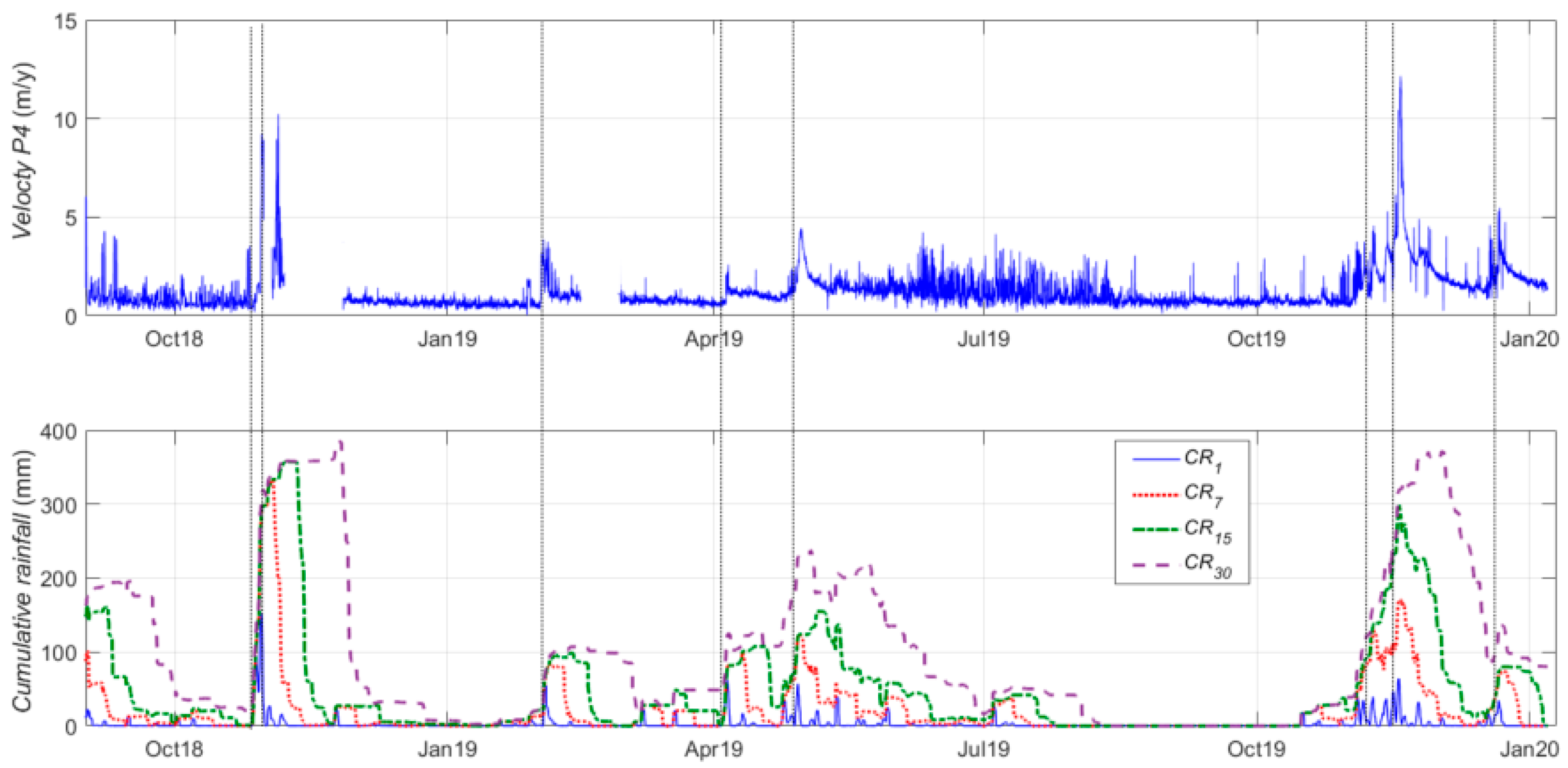
In order to establish if the proposed method can be applied in the specific case, it is essential to verify that the landslide motion is driven by rainfall. The comparative analysis between the velocity and 1 d ($C{R}_1$), 7 d ($C{R}_7$), 15 d ($C{R}_{15}$), and 30 d ($C{R}_{30}$) cumulative rainfall distributions was carried out for all the reflectors. Figure 7 shows the data about P4, located in the Area 2 center. The other reflectors in this area have similar behavior. The main results are the following:

• The landslide kinematics is always driven by rainfall. An analysis of the cross-correlation between rainfall and velocity time series highlights that the delay of the kinematical response to a rainfall stimulus typically ranges from 12 to 36 h. The reaction delay decreases when an episode of heavy rainfall occurs during a rainy period;
• In case of rainfall, the velocities can increase 3–5 times with respect to the values in the absence of rainfall and, in some cases, the increases can reach 10–15 times;
• Extreme phenomena, with material falling, are due to either episodes of high intensity rainfall ($C{R}_1>150 \mathrm{mm}$) occurred in a very short time (1–2 d), as in the case of “Vaia” storm occurred on 29 October 2018 [30], or periods of 10 to 15 days of medium intensity rainfall ($C{R}_1$ no more than 40–60 mm), as occurred in November 2019;
• Periods characterized by high average velocity and oscillations are followed by relaxation periods lasting from a few weeks to a few months in which a velocity similar to the initial one is recovered. However, the recovery is not total, but the final mean velocity is usually 5–10% higher than the initial one, leading to progressively higher velocities. Other landslides show a similar behavior [31];
• Extreme events mainly occur in the autumn and spring, which are particularly rainy periods. The movements of the landslide are usually reduced in periods of frost.

These results show that, in order to take into account the effects of both long rainy periods and high-intensity episodes (within a rainy period or not), a really useful forecasting system must be able to capture the behavior of the unstable slope with an hourly resolution for at least two weeks.

3.3. Forecasting System and Results

The system based on the proposed method should provide early forecasts of the velocity trend in Area 2. Since an inspection of the RTS data revealed that the kinematic behavior of the landslide significantly changed in 2017, the data obtained in the period from 1 January 2018 to 8 December 2020, which corresponds to approximately 25,800 hourly observations for each reflector, were used for the CNN training. For each reflector in Area 2, the velocity at a given time $t_c$ was computed as the slope of the least square straight line of positions in the time span from $t_c-1 \mathrm{d}$ and $t_c$ after the deletion of possible spikes by means of moving average filtering. A single velocity $v(t_c)$ was obtained by taking the mean of the reflector velocities.

The following parameters were chosen in this way:

• $N_{A }=15 \mathrm{d}$ because extreme phenomena, with fall of material with volume of some cube meters, are due to either episode of high intensity rainfall (cumulative day rainfall occurred in a very short time or periods of 10 to 15 days of medium intensity rainfall (see Section 3.2, number 3);
• $N_B=0$ because no reliable quantitative rainfall forecasts were available;
• $N_C=N_D=5 \mathrm{d}$ because the kinematical response time to rainfall stimuli was typically in the range from 12 h to 3 d (Section 3.2, number 1);
• $V_H=21 \mathrm{mm}/\mathrm{h}$ (i.e., 7.5 m/y) because material fall from the unstable slope, with typical involved volume of a few cube meters, occurred when the velocity reached this value;
• $V_M=7 \mathrm{mm}/\mathrm{h}$ (2.5 m/y) because the recovery of the velocity before the triggering, i.e., ~2.2 mm/d (~0.8 m/y) was fast (up to three days) if the maximum velocity was below this value but required a more or less long relaxation period (several days, weeks, or months) it this value was exceeded.

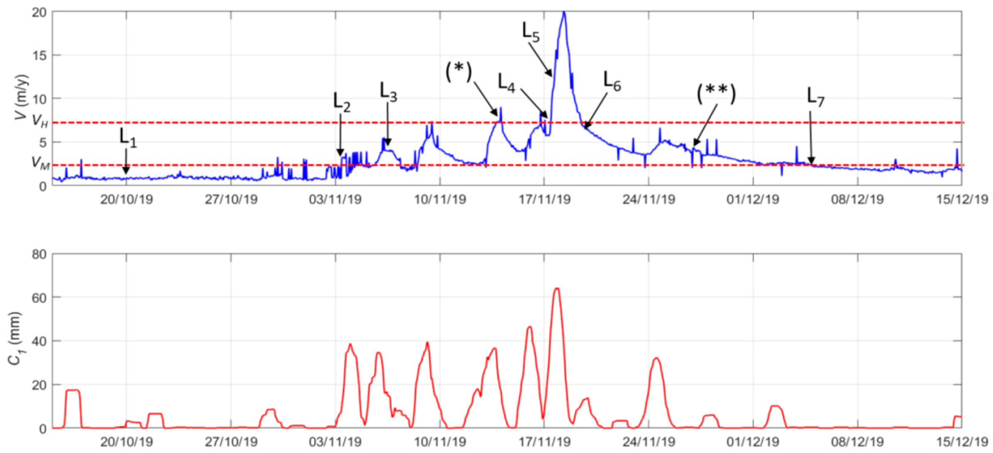
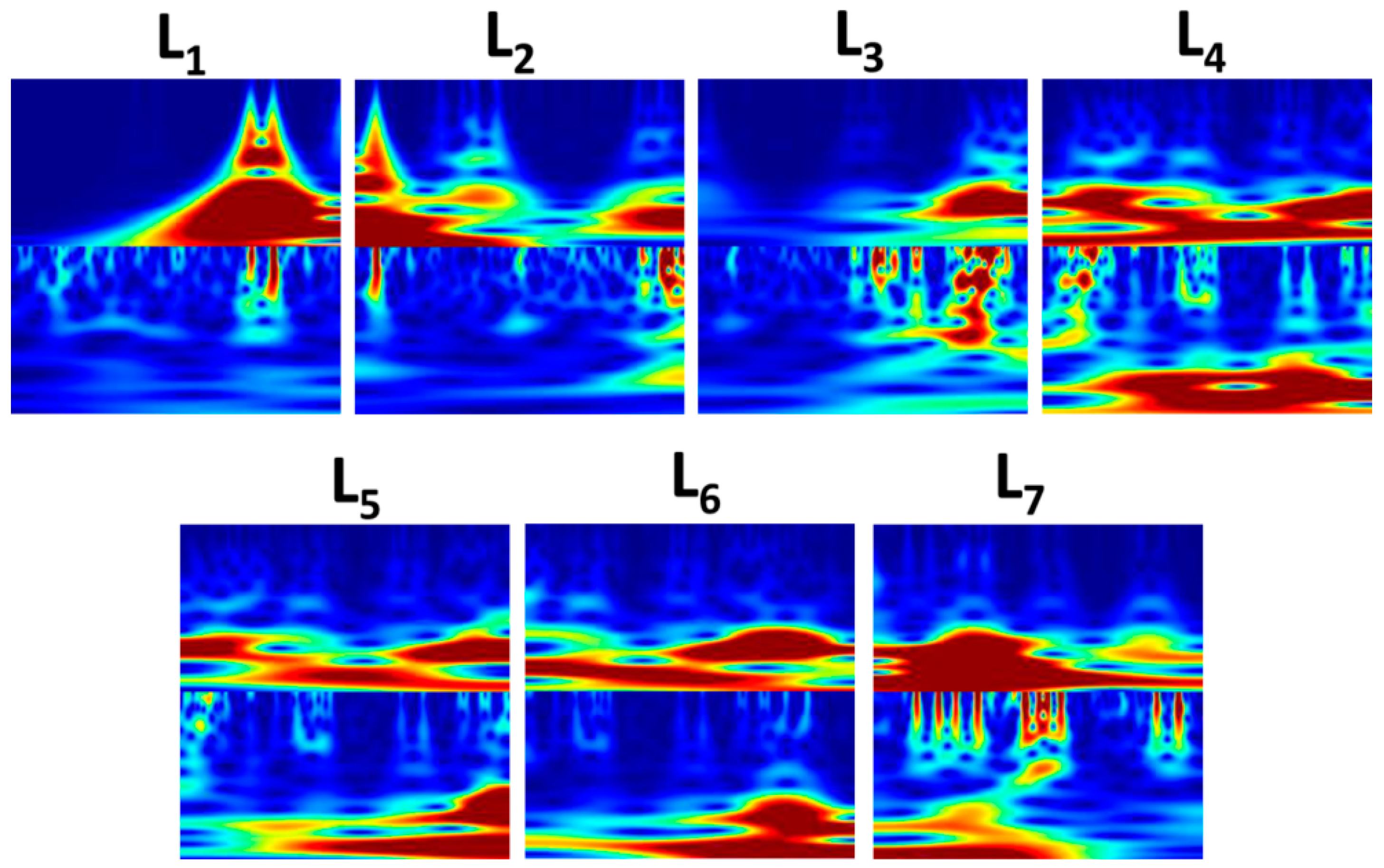
The rainfall and velocity time series in the time span from 15 October to 15 December 2019 are shown in Figure 8, where an event for each possible trend L₁–L₇ is highlighted. The corresponding scalograms are in Figure 9.

Table 2. Amount of scalogram images before and after data augmentation and their subdivision into datasets for training, validation, and test of the convolutional neural networks (12 computation times per day).

Condition	Scalogram Images
	Before DA 1	After DA 1	Training (60%)	Validation (20%)	Test (20%)
U 2	36	-	-	-	-
L1	5890	2524	1514	505	505
L2	901	901	541	180	180
L3	2524	2524	1514	505	505
L4	556	1967	1181	393	394
L5	245	2278	1367	456	456
L6	362	2161	1297	433	432
L7	857	857	514	172	171
Total	11,371	13,212	7928	2644	2643

¹ DA states for data augmentation. ² U states for undefined trend.

summarizes the number of available events in the period from January 2018 to January 2020 as a result of the training-aimed trend labeling, as well as the number of events after the data augmentation and their subdivision into training, validation, and test datasets. The data augmentation was performed by adding a zero-centered Gaussian noise to the time series inherent to outputs L₄, L₅, and L₆. The SDs of the used Gaussian noise were 9 mm for the rainfall time series and 2 mm/d (0.7 m/y) for the velocities, which are similar to the SDs of the corresponding observed time series.

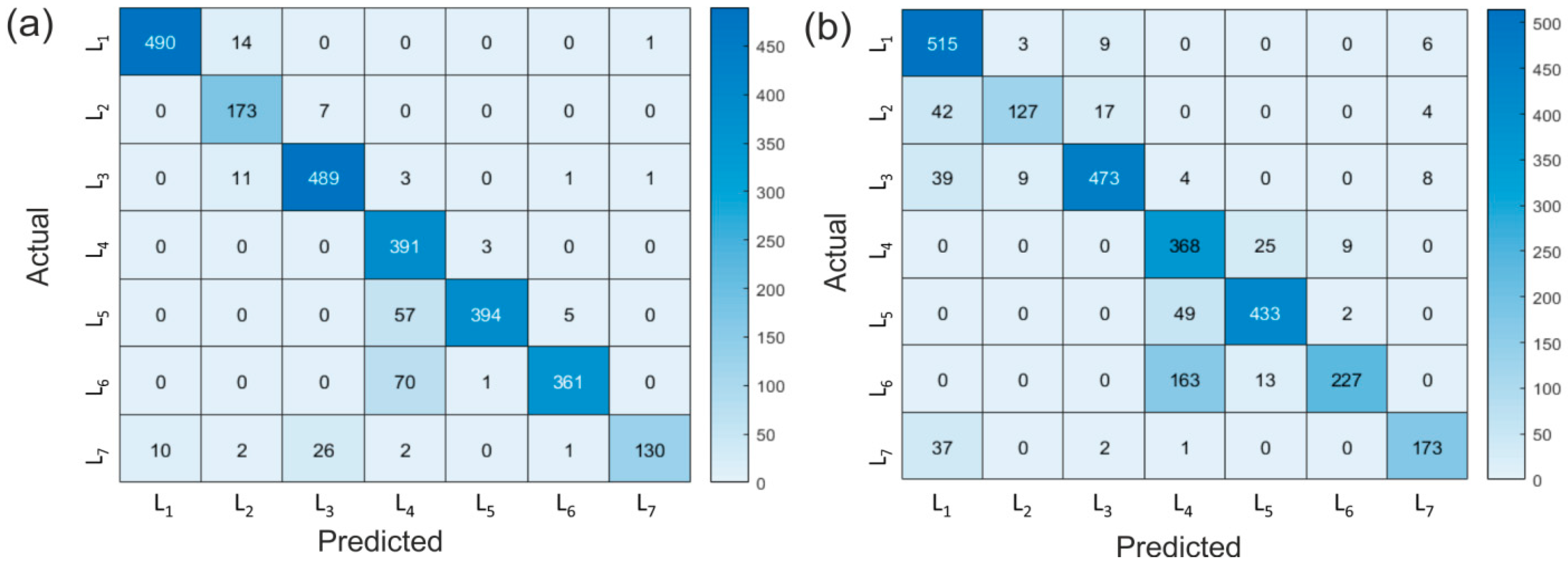
The training, based on a pre-trained VGG19 [11], was carried out for both the proposed CNN configurations; one with rainfall and velocity scalograms and one with rainfall scalograms only. The confusion matrix summarizes the performance of a CNN by showing how many events of a class are correctly classified by the CNN and how many are classified in other classes instead. The confusion matrices of the two trained CNNs are shown in Figure 10. If both rainfall and velocity scalograms are used (Figure 10a), the forecasting system has good performance; 391 (99.2%) of the 394 actual L₄ trends (mid/high-velocity transition) are correctly classified, and 3 (0.8%) are classified as L₅ (high velocity), and more importantly, no actual L₄ trends are classified as L₃ (mid velocity). This is a remarkable achievement because a missed alarm, as would be the case of actual L₄ trends classified as L₃, could cause immediate problems. Since 490 (97%) of the 505 actual L₁ trends (low velocity) are correctly classified, 14 are classified as L₂ (low/mid-velocity transition), and 1 only as L₇ (mid/low-velocity transition), undue pre-alarm signals are unlikely. Since no more than 3 (0.6%) of the 515 L₃ trends are classified as L₄, undue alarm signals are highly unlikely. The CNN trained with rainfall scalograms only (Figure 10b) has a lower performance; 368 (92%) of the 402 actual L₄ trends are correctly classified, and 25 (6%) are classified as L₅, 9 (2%) as L₆, and zero as L₃. However, the fact that such a second CNN is used only in the case of the absence of velocity data should be taken into account.

The computations were carried out by means of a notebook equipped with an Intel^® Core^® i7-3630QM CPU, 2.40 GHz clock, NVIDIA^® GeForce GT 650M graphic card equipped with CUDA^® platform, and 16 GB RAM. The elapsed times were 5 min for the complete rainfall-velocity scalogram generation and 10 h for the corresponding CNN training and validation for each configuration. An operation session takes about one minute, including access to the database and sending the email with the forecast.

4. Discussion and Conclusions

The proposed toolbox is aimed at predicting the landslide velocity trend for a period of some hours to one or two days and providing the results to persons involved in decision making. The main result is that a CNN based on rainfall and velocity scalograms is characterized by very good performance (Figure 10a) and could be included in an automated landslide monitoring/early warning system. As pointed out by [2], the forecasting systems based on rainfall information only are not much used to provide slope-scale forecasts. The procedure proposed here integrates rainfall and velocity data and, therefore, constitutes an innovation in the panorama of landslide monitoring. In the L₄ case, the predictions are very good, showing that missed alarms are very unlikely. Moreover, even if 12% of the L₅ trends are classified as L₄, this is not a problem because they are transitions to be confirmed. No more than 0.8% of L₅ scalograms are classified as L₆. It should also be noted that false alarms (trends L₁ recognized as L₃, L₄, or L₅), which could be harmful because a series of false alarms could lead to underestimating true alarms in the future, do not occur. The cases L₆ and L₇ are also significant since returning from an emergency condition is an important task for a decision maker. In these cases, the performance is lower (poor in the case of L₇), but this is not a true problem because the precautionary principle implies that a trend classified as L₆ or L₇ must be considered as information to be taken into account later if confirmed by next L₃ or L₁ values, respectively. As expected, the performance of the CNN with velocity and rainfall scalograms is significantly better than that of the CNN based on rainfall scalograms alone.

A single velocity time series was used in the specific application. This is because the Perarolo landslide is characterized by two well-defined kinematic areas, and the primary objective of monitoring is to study the possible evolution of Area 2. If the studied, unstable slope has complex kinematics, it may be necessary to evaluate the velocity time series of several areas. If this occurs, a couple of CNNs must be implemented for each of these areas.

An important issue concerns the maximum term for a reliable forecast. Obviously, for $t>t_c+N_D$ the system does not provide forecasts. A relatively large $N_C+N_D$ (10 d for Perarolo landslide) has above all the purpose of having a large statistic to correctly estimate the trend during training. In the operational phase, the CNN provides a reliable trend centered on $t_c$ for a period of no more than ~1–2 d. However, it should be noted that the system continues to provide upgraded forecasts according to the frequency set by the operating system’s task manager, e.g., 6 or 12 times per day.

A possible criticism of the method is related to the fact that in the operational phase, significant and unexpected variations over time of the spectral content of the rainfall and, above all, velocity-time series could occur. However, one of the major advantages of a well-trained neural network is its ability to generalize, i.e., its ability to classify data from the same class as the learning data that it has never seen before. Moreover, when calculating the scalograms, the cumulative rainfall and the reached velocities, as well as their fluctuations, can also be calculated. An incorrect prediction (for instance, an L₄ episode reported as L₁ or L₇) would thus be immediately recognized. Furthermore, an intentionally exaggerated data augmentation, i.e., based on exaggerated rainfall and velocity SDs, could be used to account for possible episodes characterized by anomalous spectral content.

The real-time data on pore pressure, water table, or other information on the soil were not available in the test landslide. However, their indirect effects are considered because the combined use of CWT and CNN on rainfall and velocity time series makes it possible to consider, if the training is performed on an adequate amount of data, the different responses to the rainfall stimulus based on the ground conditions. The results show that, provided that the kinematics is rainfall-driven, it is possible to obtain predictions with the proposed method. If data on pore pressure, soil moisture, or other quantities that can affect the landslide kinematics are monitored, they should be integrated into the forecasting system. The current version of the WADENOW toolbox can already be used with time series of pore pressure, i.e., the images sent to the CNN can show scalograms of velocity and pore pressure instead of velocity and rainfall. In the event that time series of velocity, rainfall, and pore pressure are available, two CNNs must be trained, one for the velocity/rainfall couple and the other for the velocity/pore pressure couple. Experiments are needed in a real case to evaluate how to weigh the forecasts of two or more CNNs to obtain a single forecast. Another possibility, in the case of three-time series, is the generation of images with three scalograms. This would allow the use of a single CNN. However, the fact that the images to be sent to a CNN must be 224 × 224 or 227 × 277 means that increasing the number of variables could cause a worsening of the resolution in frequency. A third possibility is the use of a multiple-input/single-output CNN [32], which, however, would require training from scratch. In any case, the use of several variables requires adequate experimentation and is a development of the method currently under study.

The application of the proposed method to a debris flow or another phenomenon characterized by extremely rapid variation requires experimentation and possible adaptations because there could be a problem of having enough data to allow CNN training.

The computational cost of CNN training is fully compatible with the resources currently available, especially if GPU-accelerated computations are carried out. The calculation and transmission of a forecast take no more than a minute.

All the scripts are accessible to the user for possible customization or translation into the Python language by using the open-source PyWavelets and Keras libraries.

In conclusion, the proposed methodology is ready-to-use, flexible, and applicable to a wide range of slope instability phenomena whose kinematics are driven by rainfall. The output forecasts could be used by a decision-making body devoted to hydrogeological risk management.