Article

Emergence of Algal Blooms: The Effects of Short-Term Variability in Water Quality on Phytoplankton Abundance, Diversity, and Community Composition in a Tidal Estuary

by
Todd A. Egerton
1,*,
Ryan E. Morse
2,†,
Harold G. Marshall
1 and
Margaret R. Mulholland
3,†
1
Department of Biological Sciences, Old Dominion University, Norfolk, VA 23529, USA
2
Graduate School of Oceanography, The University of Rhode Island, Narragansett, RI 02882, USA
3
Department of Ocean, Earth and Atmospheric Sciences, Old Dominion University, Norfolk, VA 23529, USA
*
Author to whom correspondence should be addressed.
These authors contributed equally to this work.
Microorganisms 2014, 2(1), 33-57; https://doi.org/10.3390/microorganisms2010033
Submission received: 24 September 2013 / Revised: 28 October 2013 / Accepted: 28 November 2013 / Published: 8 January 2014

Abstract

:
Algal blooms are dynamic phenomena, often attributed to environmental parameters that vary on short timescales (e.g., hours to days). Phytoplankton monitoring programs are largely designed to examine long-term trends and interannual variability. In order to better understand and evaluate the relationships between water quality variables and the genesis of algal blooms, daily samples were collected over a 34 day period in the eutrophic Lafayette River, a tidal tributary within Chesapeake Bay’s estuarine complex, during spring 2006. During this period two distinct algal blooms occurred; the first was a cryptomonad bloom and this was followed by a bloom of the mixotrophic dinoflagellate, Gymnodinium instriatum. Chlorophyll a, nutrient concentrations, and physical and chemical parameters were measured daily along with phytoplankton abundance and community composition. While 65 phytoplankton species from eight major taxonomic groups were identified in samples and total micro- and nano-phytoplankton cell densities ranged from 5.8 × 10⁶ to 7.8 × 10⁷ cells L−1, during blooms, cryptomonads and G. instriatum were 91.6% and 99.0%, respectively, of the total phytoplankton biomass during blooms. The cryptomonad bloom developed following a period of rainfall and concomitant increases in inorganic nitrogen concentrations. Nitrate, nitrite and ammonium concentrations 0 to 5 days prior were positively lag-correlated with cryptomonad abundance. In contrast, the G. insriatum bloom developed during periods of low dissolved nitrogen concentrations and their abundance was negatively correlated with inorganic nitrogen concentrations.

1. Introduction

In estuarine systems, phytoplankton communities are highly variable, affected by numerous environmental and ecological factors including water temperature, salinity, light intensity, nutrient availability, inter- and intra-specific competition among the algae, and predation [1,2,3,4]. Many of these environmental factors vary on short time scales in estuaries due to tidal and diel fluctuations in physical/chemical parameters and episodic nutrient inputs from precipitation events [5,6,7,8]. Because of their short generation times, phytoplankton populations can respond rapidly to environmental and ecological forcing [9,10,11] Consequently, changes in algal community composition and diversity can occur over relatively short time periods in response to environmental variability [12,13,14] and this can affect ecological function [15,16].
Algal blooms usually involve rapid changes in phytoplankton community composition, where in phytoplankton communities become dominated by a single (or a few) species over the course of days, resulting in nearly monospecific assemblages that can then persist for weeks to months [17,18]. Such monospecific algal blooms appear to be increasing in frequency and magnitude, and nutrient over-enrichment has been implicated as a causal factor [19,20]. However, linking blooms to a proximate trigger has proven difficult because blooms are generally sampled only after they become visible when cell densities are already high enough to discolor water. As a result, the environmental conditions during bloom initiation are usually unknown. In addition, bloom organisms can be transported from sites of initiation to the areas where algal biomass accumulates and blooms are observed [21].
Because environmental conditions and phytoplankton communities can change rapidly in estuaries due to physical and meteorological forcing, monthly monitoring is not sufficient to document bloom initiation in response to short-term environmental variability. Recent studies aimed at identifying causal factors promoting bloom formation sampled more frequently and demonstrated that rapid changes in algal biomass as blooms developed and then dissipated associated with short-term variability in water quality [7,8,22,23]. Continuous monitoring and high resolution mapping has further highlighted the rapid fluctuations and spatial variability in nutrient and dissolved oxygen concentrations, chlorophyll biomass, temperature and salinity over diurnal timescales [7,21,24]. Daily sampling studies have also been used to document the relationships between water quality parameters and algal community composition that occur over short periods of time [7,12,25]. These studies suggested that meteorological forcing was important in driving changes in algal community structure.
The objectives of this study were to identify short-term changes in phytoplankton species composition and diversity and relate these with water quality parameters and meteorological forcing, the development of mono-specific blooms, and algal species diversity in a tidal estuarine system during spring, when rainfall is usually frequent and the algal community diverse.

2. Experimental Section

2.1. Study Site

The Lafayette River, located in Norfolk, VA, USA, is a tributary of the Elizabeth River that flows into the lower James River near its confluence with the Chesapeake Bay. It is a tidal river, approximately 8 km in length, with a mean depth of 1.3 m, and a maximum channel depth of 7.6 m [26]. The river is surrounded by residential and commercial development, within an urban watershed of 43.28 km2, and a shoreline that includes bulk headed regions, marinas, private docks and wetland marshes of Spartina alterniflora [26,27,28,29]. Freshwater input is delivered through precipitation and shoreline drainage that includes 13 storm sewers and overflow drains [27,30]. Seasonal dinoflagellate blooms common in this river include: Prorocentrum minimum (early spring) and Akashiwo sanguinea and Cochlodinium polykrikoides (summer and fall) [22,31,32,33]. The river has been identified as an initiation site for regional dinoflagellate blooms dominated by C. polykrikoides during summer and fall [20].

2.2. Methods and Materials

Surface water samples were collected once a day during the incoming tide, approximately 2 h after low tide, from a stationary floating dock on the Lafayette River between 20 April and 25 May 2006, as described by Morse et al. [7]. The mean water depth at the station was 0.9 m. Water temperature, salinity, pH, and dissolved oxygen were measured daily just before collecting water samples using a Hydrolab Data Sonde 4a water quality multiprobe (Hach Company, Loveland, CO, USA). Rainfall and air temperature were recorded at Norfolk International Airport, <10 km from the Lafayette River station.
Samples (25–50 mL) were collected onto Whatman GF/F filters (pore size ~0.7 μm) and frozen for later analysis of chlorophyll a (Chla). Chla was measured fluorometrically after extraction in acetone within 2 weeks of sample collection [34]. Samples were filtered through 0.2 μm Supor filters and the filtrate frozen for later analysis of dissolved nutrient concentrations. Dissolved nitrate, nitrite, urea, phosphate, and silicate were measured colorimetrically using an Astoria Pacific nutrient autoanalyzer according to the manufacturer’s specifications. Ammonium was analyzed colorimetrically using the phenolhypochlorite method [35].
Nano- and microphytoplankton samples (500 mL) were collected from the surface (<1 m), preserved with Lugol’s solution (1% final concentration), and quantified using an inverted microscope (Nikon TS100) at 150–600× magnification following a modified Utermöhl settling and siphoning protocol [36]. Autotrophic picoplankton samples, collected at the same time and depth were preserved with gluteraldehyde (2%) and quantified using epifluorescence microscopy (Nikon E600) at 1000× magnification [37]. Phytoplankton cell volume was calculated based on observed cell dimensions and phytoplankton carbon (C) biomass calculated using established biovolume to biomass relationships [38]. Dinoflagellate species identities were positively confirmed using scanning electron microscopy (SEM). Samples for SEM were fixed with gluteraldehyde and osmium tetroxide, dehydrated through an ethanol series, dried using a critical point drier, sputter-coated with gold-paladium, and analyzed using a LEO 435VP (LEO Electron Microscopy Ltd., Thornwood, NY, USA) [39]. Phytoplankton diversity was calculated daily using both species richness (number of species per sample) and the Shannon index (H′; Equation (1)), the latter incorporates the relative abundance of each species and therefore is commonly used as a measure of species evenness [40].
Microorganisms 02 00033 i001
pi is the proportion of the total algal biomass of species i.
The daily sampling regimen was designed to measure phytoplankton species abundance and nutrient concentrations prior to, during, and following algal blooms. Phytoplankton species abundance and diversity were compared with corresponding environmental data using Pearson correlation analysis. Because algal growth rates are on the order of days, we anticipated a lag response of phytoplankton abundance relative to nutrient concentrations and associated meteorological forcing [7]. The lag correlation analyses conducted here compared nutrient concentrations at one day intervals over an 11 day window encompassing the period before and after observed blooms of a cryptomonad and the dinoflagellate, Gymnodinium instriatum. Because biological interactions such as competition and predation are known to influence phytoplankton composition, we also used a lag correlation analysis of species richness, H′, and the abundance of other dominant phytoplankton groups relative to dinoflagellate and cryptomonad abundance.
Regression analysis was used to examine the relationship between species diversity (both richness and H′) and total algal biomass. These results were compared to regression analyses of phytoplankton diversity and biomass data collected by the authors from nearby sites during the same time period as part of the Virginia Chesapeake Bay monitoring program (n = 26). Because previous studies identified both linear and non-linear (unimodal) relationships between the variables (e.g., [41]), analysis of variance was conducted to test for significant linear and quadratic relationships using regression models (SPSS 20; IBM). If both regression models were significant for a particular analysis, a partial F test was used to determine if the quadratic model significantly improved the explanation of the data relative to the linear model [42,43].

3. Results and Discussion

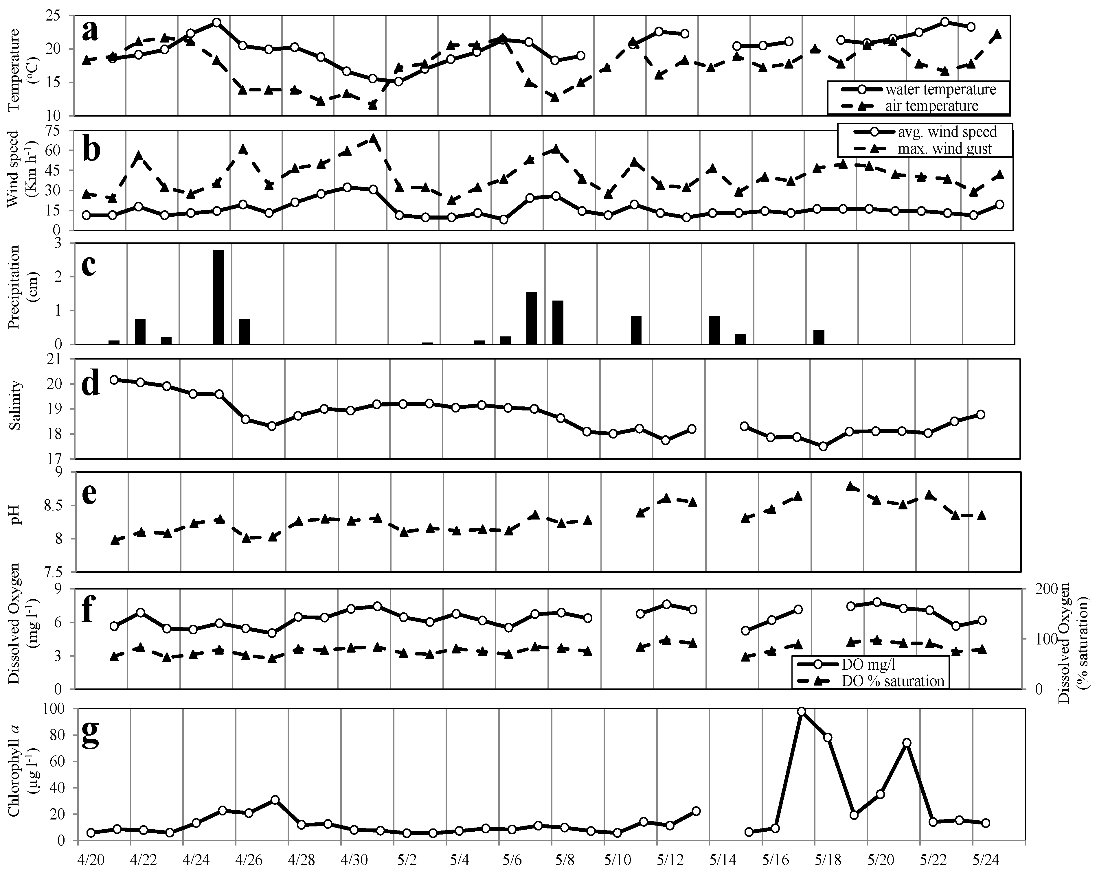
3.1. Meteorological and Physical Parameters

Over the 34-day sampling period, mean daily air temperatures ranged from 11.7 to 21.7 °C, and water temperatures ranged from 15.1 to 24.0 °C (Figure 1a). Average daily wind speeds were variable and ranged from 8 to 32 km h−1 with gusts exceeding 48 km h−1 (30 miles h−1) on 9 days; maximum wind gusts of 69 km h−1 were observed on May 1 (Figure 1b). During the sampling period there were 8 rain events recording 0.5 cm or more of precipitation (Figure 1c). Salinity at the sampling site decreased over the sampling period, with a maximum of 20.2 observed on 20 April and a minimum of 17.5 on 18 May. Salinity decreased following periods of rainfall (Figure 1d). The average pH at our study site was 8.31, but pH ranged from 7.98 to 8.79 (Figure 1e). Dissolved oxygen concentrations ranged from 5.0 to 7.8 mg L−1; this was 61.6% to 98.1% saturation (Figure 1f).
Figure 1. Daily measurements of physical and chemical parameters in the Lafayette River from 20 April to 25 May 2006. Water temperature (°C) was measured at the sampling site using the Hydrolab and mean daily air temperatures were measured at Norfolk International Airport (ORF) (a). Mean daily wind speed and maximum daily speed of wind gusts (miles h−1) were measured at Norfolk International Airport (ORF) (b). Daily cumulative precipitation (cm) was also measured at ORF (c). Salinity (d), pH (e), dissolved oxygen (mg L−1), and percent saturation (f) were measured using the Hydrolab and chlorophyll a measurements (µg L−1) were made daily on surface water samples (g).
Microorganisms 02 00033 g001

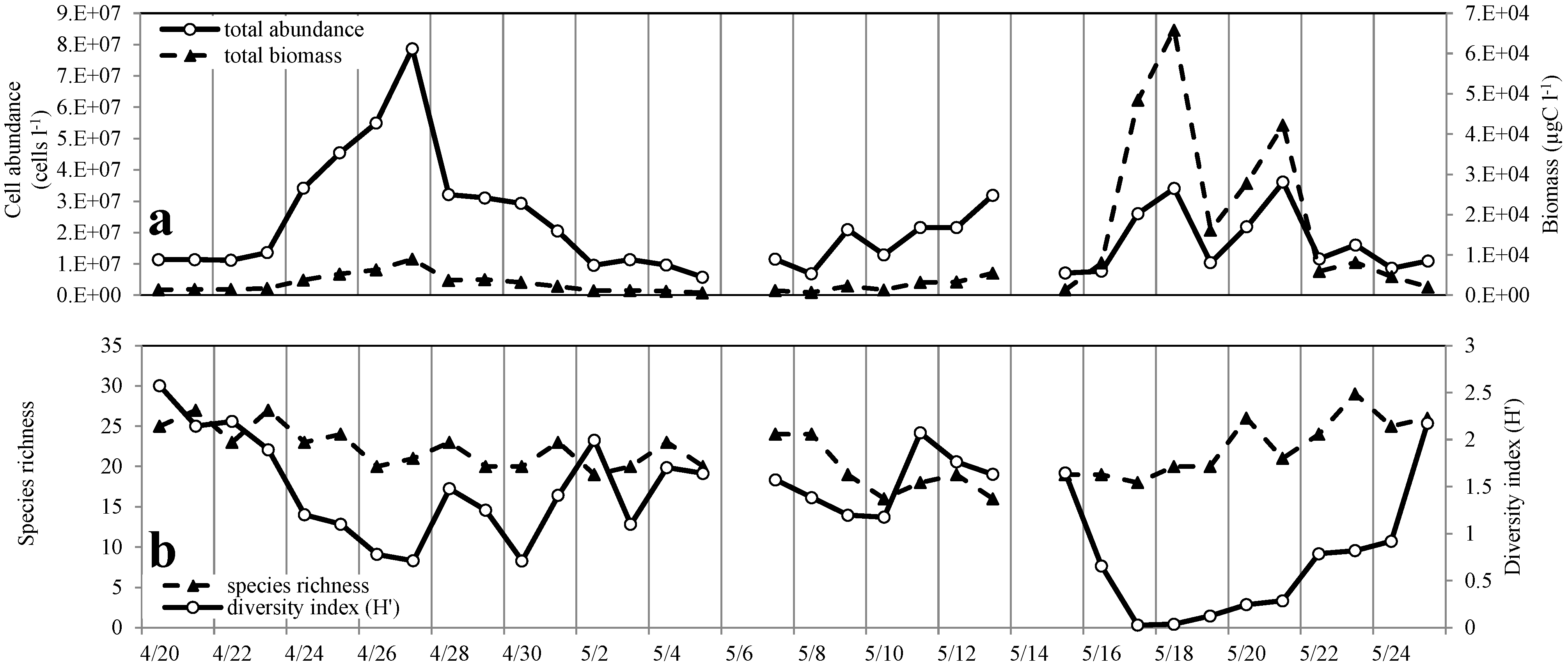
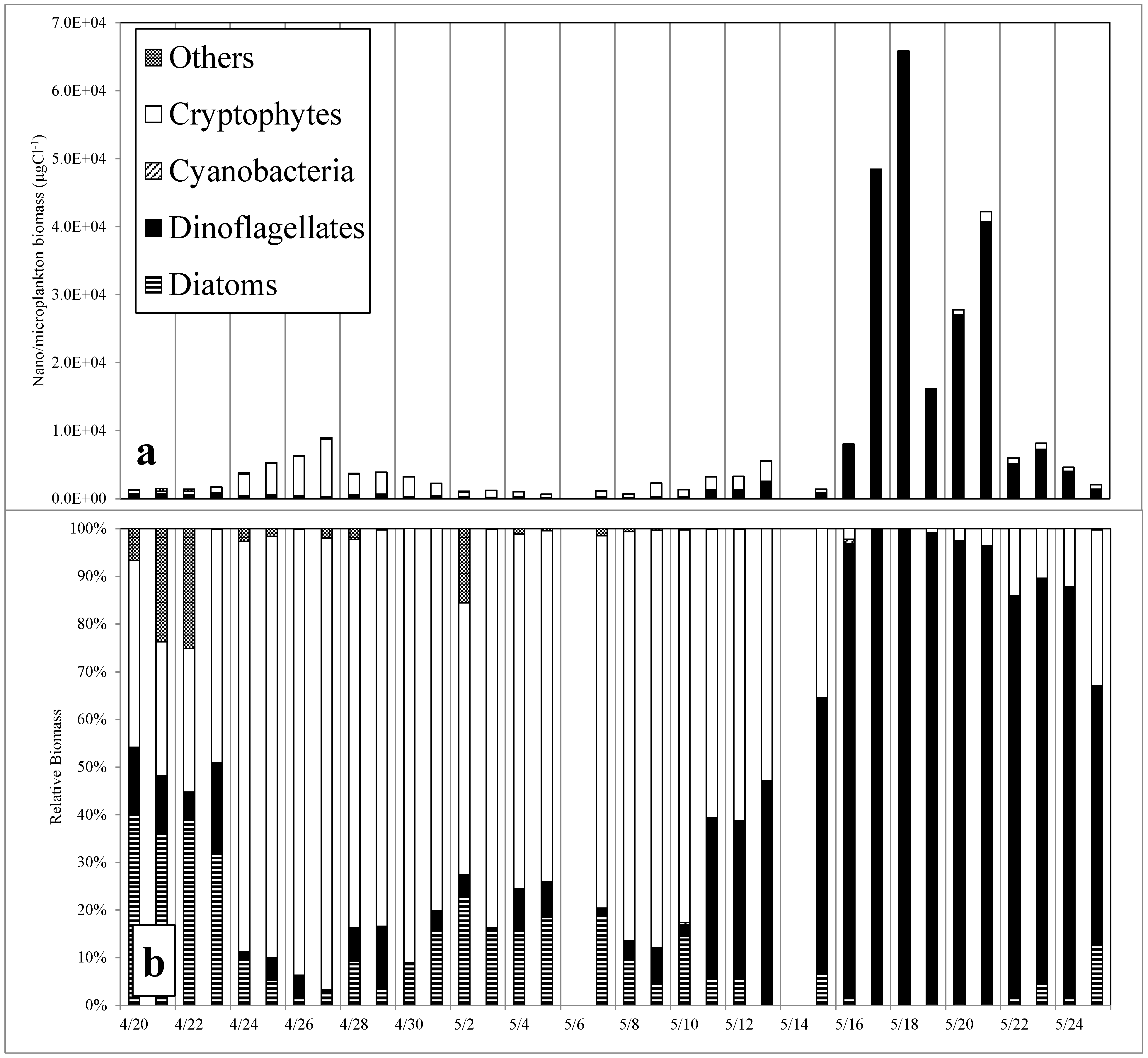
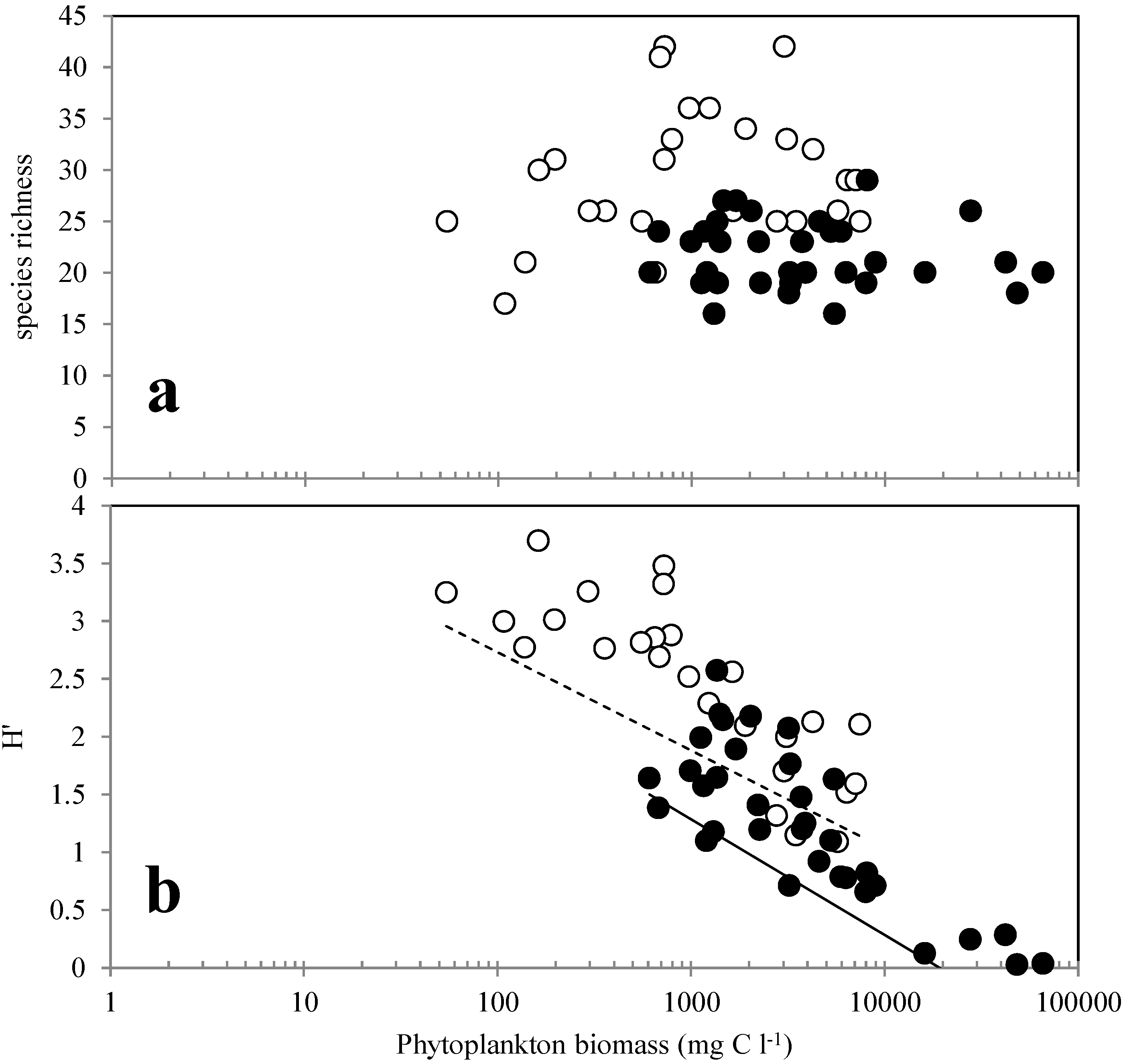
3.2. Phytoplankton Abundance, Composition and Diversity

Chlorophyll a (Chla) concentrations ranged from 5.54 to 97.6 µg L−1 over the 34-day study period, but were less than 20 µg L−1 for all but 8 of the days (Figure 1g). Elevated Chla concentrations, 20.8–30.7 µg L−1, observed between 24 April and 1 May, were associated with a cryptomonad bloom (Figure 1g). High Chla concentrations observed between 16 and 24 May (35.2–97.6 µg L−1) were associated with high abundances of the dinoflagellate Gymnodinium instriatum (Figure 1g). Nano- and microphytoplankton cell densities ranged from 5.8 × 10⁶ to 7.8 × 10⁷ cells L−1 throughout the study period (Figure 2a); picoplankton abundances ranged from 3.7 × 10⁶ to 1.3 × 10⁹ cells L−1 (data not shown).
Figure 2. Nano and micro phytoplankton abundance and biomass (a), and phytoplankton diversity (Shannon diversity index H′) and species richness (b) in daily samples collected from the Lafayette River between 20 April and 25 May 2006.
Microorganisms 02 00033 g002
While dominated by a single species during blooms, the phytoplankton community consisted of 65 taxa from 8 major taxonomic groups, with 41 taxa present on 5 or more days (Table 1). There were 37 species of diatoms, 17 dinoflagellate species, 3 cyanobacteria, 2 silicoflagellates, 2 chlorophytes, and 1 each of cryptomonads, euglenophytes and prasinophytes. While diatoms were the most diverse group, consisting of mainly centric species (e.g., Skeletonema costatum and Chaetoceros spp.), they never represented more than 49% of the total phytoplankton present, and were generally much less abundant than the phytoflagellates.
Table 1. Summary statistics of phytoplankton abundance data (cells L−1) of the 41 taxa observed in the Lafayette River samples at least 5 times during the study. The two bloom taxa are identified in bold.
Phytoplankton TaxaAbundance
Mean ValueMinimum ValueMaximum Value
Diatoms
unidentified Centrales 10–30 µm2.0 × 1061.0 × 1035.3 × 106
unidentified Centrales 30–60 µm1.0 × 1042.6 × 1021.1 × 105
Chaetoceros pendulus6.7 × 1022.6 × 1021.0 × 103
Chaetoceros sp.1.2 × 1057.7 × 1024.3 × 105
Cocconeis sp.2.8 × 1022.6 × 1025.1 × 102
Coscinodiscus sp.5.7 × 1022.6 × 1021.3 × 103
Cyclotella sp.1.1 × 1055.1 × 1024.3 × 105
Cylindrotheca closterium5.3 × 1022.6 × 1021.5 × 103
Dactyliosolen fragilissimus2.9 × 1045.1 × 1023.2 × 105
Gyrosigma fasciola3.1 × 1022.6 × 1025.1 × 102
Leptocylindrus minimus7.7 × 1047.7 × 1025.4 × 105
Navicula sp.7.3 × 1022.6 × 1023.8 × 103
Nitzchia sp.2.6 × 1022.6 × 1022.6 × 102
unidentified Pennales 10–30 µm2.6 × 1052.6 × 1028.7 × 105
unidentified Pennales30–60 µm8.9 × 1032.6 × 1021.1 × 105
unidentified Pennales > 60 µm9.0 × 1022.6 × 1022.8 × 103
Pleurosigma sp.2.6 × 1022.6 × 1022.6 × 102
Rhizosolenia setigera1.2 × 1032.6 × 1023.8 × 103
Skeletonema costatum1.0 × 1051.0 × 1039.7 × 105
Thalassiosira sp.6.7 × 1022.6 × 1021.3 × 103
Dinoflagellates
Akashwio sanguinea3.0 × 1032.6 × 1021.8 × 104
Cochlodinium polykrikoides1.1 × 1045.1 × 1023.7 × 104
unidentified dinoflagellate1.8 × 1055.1 × 1025.4 × 105
Dinophysis punctata5.4 × 1022.6 × 1022.0 × 103
Diplopsalis lenticula3.1 × 1022.6 × 1025.1 × 102
Gymnodinium sp.8.9 × 1042.6 × 1028.7 × 105
Gymnodinium instriatum 3.7 × 1062.6 × 1023.1 × 107
Heterocapsaro tundata6.6 × 1051.1 × 1053.9 × 106
Heterocapsa triquetra1.0 × 1042.6 × 1021.1 × 105
Polykrikos kofoidii5.9 × 1031.0 × 1034.5 × 104
Prorocentrum micans9.3 × 1022.6 × 1025.9 × 103
Prorocentrum minimum2.2 × 1042.6 × 1024.3 × 105
Protoperidinium sp.7.5 × 1022.6 × 1021.8 × 103
Scrippsiella trochoidea7.3 × 1022.6 × 1022.3 × 103
Cryptomonads
Cryptomonas sp. 1.5 × 1075.4 × 1057.6 × 107
Cyanobacteria
Lyngbya sp.5.3 × 1055.1 × 1022.3 × 106
Chlorophytes
Ankistrodesmus falcatus8.7 × 1032.6 × 1021.1 × 105
Chlamydomonas sp.3.6 × 1051.1 × 1058.7 × 105
Euglenoids
Euglena sp.7.6 × 1042.6 × 1024.3 × 105
Eutreptia lanowii2.0 × 1035.1 × 1025.6 × 103
Prasinophytes
Pyramimonas sp.7.2 × 1042.6 × 1023.2 × 105
Cryptomonad taxonomic identification is notoriously problematic due to the cells’ sensitivity to chemical fixatives and the small number of morphological features that distinguish them from one another [44,45]. The morphology and size of the cryptomonads appeared consistent throughout the course of the study. The cells were comma-shaped, with a round anterior and a reflex curved pointed antapex with an average length of 18.3 μm and an average maximum width of 8.3 μm. While consistent morphological features were observed during the sampling period, the cryptomonad bloom was conservatively identified as Cryptomonas spp., indicating the possible presence of multiple species. Gymnodinium instriatum was recognized by its morphological features including the displacement of the cingulum and the shape of the apical groove (Figure 3) [46] and identified using the most recent nomenclature [47].
Figure 3. Scanning electron micrograph of a Gymnodinium instriatum vegetative cell, collected at the study site on 18 May 2006, during a bloom of this dinoflagellate. Scale bar = 10 μm.
Microorganisms 02 00033 g003
Phytoflagellates, specifically cryptomonads and dinoflagellates, were the dominant algae throughout the study. At the beginning of the study period in April, the algal community was dominated by cryptophytes and diatoms but also contained substantial populations of dinoflagellates and other species. The most abundant taxon was Cryptomonas spp., which reached a maximum density of 7.7 × 10⁷ cells L−1 on 27 April. At its peak, this group represented 96.1% of the total phytoplankton abundance and 91.6% of the phytoplankton biomass (Figure 4b). Cryptomonas spp. concentrations decreased to 4.0 × 10⁶ cells L−1 on May 5 and then increased again having a second smaller peak in abundance of 2.6 × 10⁷ cells L−1 on May 13. As the Cryptomonas spp. abundance declined, the densities of Gymnodinium instriatum rose dramatically beginning May 15. G. instriatum reached a maximum density of 3.0 × 10⁷ cells L−1 on May 18 (Figure 4a). This represented 89.8% of the phytoplankton abundance and 99.0% of the total phytoplankton biomass (Figure 4b). G. instriatum abundance and chlorophyll a concentrations decreased on May 19 following a rainfall event (Figure 1c) and then increased again to 1.9 × 10⁷ cells L−1 on May 21.
Figure 4. Biomass (µg C L−1) of the major taxonomic groups within the Lafayette River from 20 April to 25 May shown as absolute algal biomass for each major taxonomic group (a) and each taxonomic group as a percentage of the total algal biomass (b).
Microorganisms 02 00033 g004
Estimates of phytoplankton biomass made using cell abundance and biovolume were highly correlated with Chla concentrations (r = 0.95, p = 0.000). Calculated nano-and microphytoplankton biomass ranged from 609 to 65,819 µg C L−1, with the highest biomass measured during the Gymnodinium bloom from May 16 to 24 (Figure 4a). Picoplankton always contributed less than 1% of total phytoplankton biomass throughout the study ranging from 0.5 to 181 μg C L−1 throughout the study.
Species richness was low in the Lafayette River during this study, ranging from 16 to 32 with a mean of 21 taxa identified per sample compared to an average of 32 taxa identified in samples collected from the nearby Chesapeake Bay Monitoring Program station located in the Elizabeth River (SBE5) during the same time period. The Shannon diversity index (H′), which includes a measure of species evenness, ranged between 0.03 and 2.57 (Figure 2b) and was lowest during the Cryptomonas spp. and G. instriatum blooms when these species dominated the phytoplankton populations. However, even when Cryptomonas spp. and G. instriatum were at their maximum abundance and represented 96.1% and 99.0% of the biomass, respectively, there were still about 20 other phytoplankton species present and species richness did not vary during bloom and non-bloom periods. Diversity rapidly increased again after blooms dissipated (Figure 2b) and there was a significant negative linear relationship between phytoplankton biomass and diversity (H′) over the 34 day study (R2 = 0.637, p < 0.0001) (Figure 5a). A negative relationship between phytoplankton biomass and species diversity was also observed during the same time period at other locations within the lower Chesapeake Bay. No significant relationship was observed between species richness and phytoplankton biomass (p > 0.05) (Figure 5b).
Figure 5. Scatterplots of phytoplankton biomass and phytoplankton diversity expressed as species richness (a) and Shannon diversity index H′ (b). Black circles represent measurements of biomass and diversity recorded daily from samples collected in the Lafayette River from 20 April to 25 May 2006. White circles represent algal biomass and diversity measurements recorded at 14 Chesapeake Bay Program Monitoring stations in Virginia during April and May 2006. There was a significant negative linear relationship between species diversity and phytoplankton biomass for both datasets (p < 0.0001) (b). The solid line shows the relationship for the Lafayette River samples and the dashed line shows the relationship for the Chesapeake Bay Program data.
Microorganisms 02 00033 g005

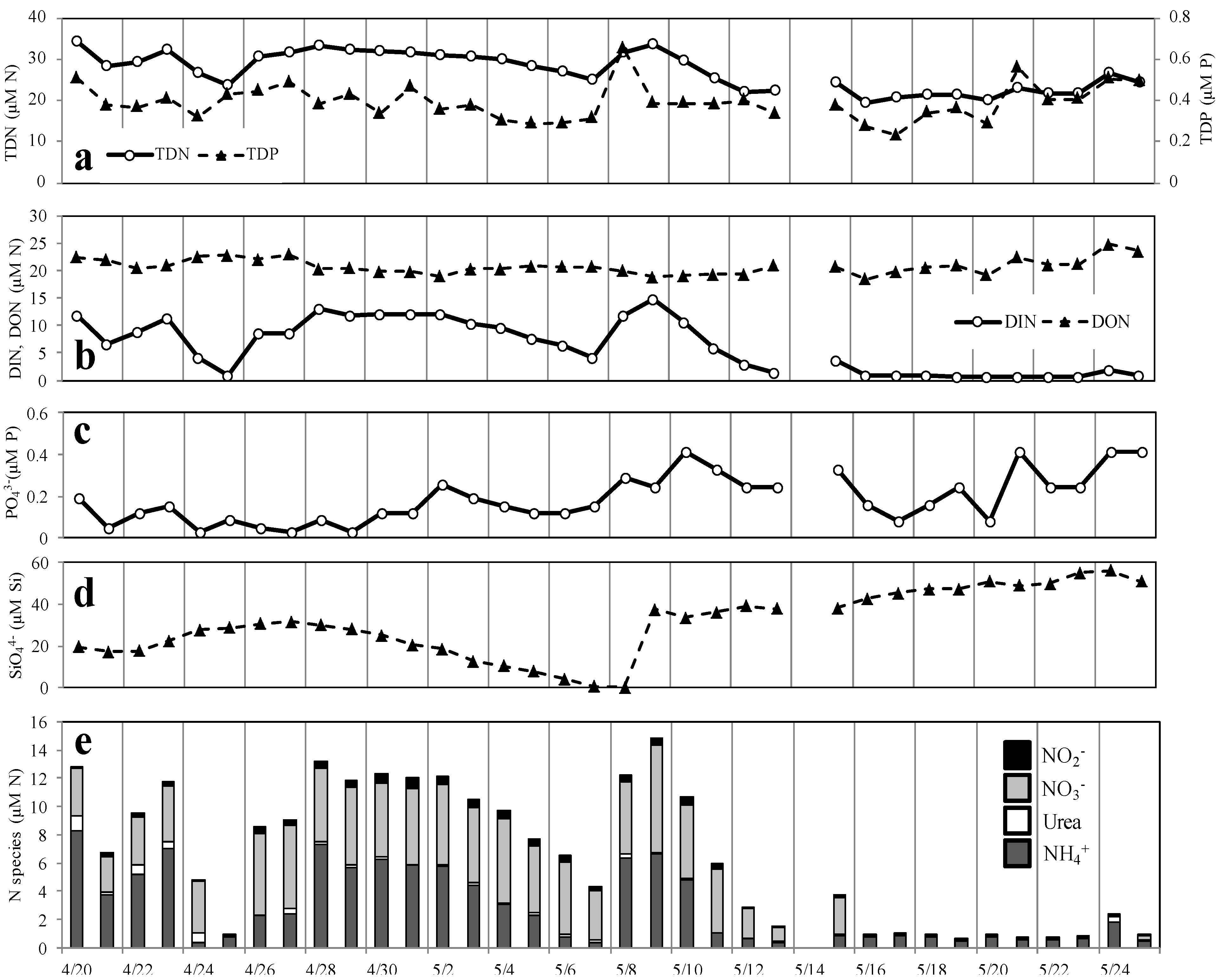
3.3. Nutrient Concentrations

Dissolved inorganic nitrogen concentrations (DIN) (nitrite, nitrate, and ammonium) ranged from 0.54 to 14.7 µM during the study period. DIN concentrations were highest at the start of the study and lowest after May 16 when dinoflagellate abundances were highest (Figure 6b). While nitrate and ammonium were both abundant during the early part of the study period, after May 15, about the time of the dinoflagellate bloom, nitrate concentrations were depleted and only ammonium was detected.
Figure 6. Nutrient concentrations measured in the Lafayette River from 20 April to 25 May 2006. Daily measurements of total dissolved nitrogen (TDN, µM N) and total dissolved phosphorus (TDP, µM P) (a), dissolved inorganic nitrogen (DIN, µM N) and dissolved organic nitrogen (DON, µM N) (b), orthophosphate (µM P) (c), dissolved silicate (µM Si) (d), and dissolved nitrogen concentrations by species (e).
Microorganisms 02 00033 g006
Nitrate concentrations ranged from the detection limit (0.05 µM) during and after the Gymnodinium (May 16 to May 24) bloom to 7.6 µM during the period between the two blooms, and represented a large portion of the available DIN, averaging 41% of the DIN pool over the study period (range was detection limit to 88% of DIN) (Figure 6e). NO3 was generally present at high concentrations (>1 μM) until May 16 and then NO3 was depleted in the days leading up to the dinoflagellate bloom, during the latter part of the study period. NO3 concentrations remained low subsequent to the G. instriatum bloom. NO2 concentrations were always <1 μM and accounted for less than 10% of the DIN pool throughout the study; the maximum NO2 concentration was 0.81 µM (Figure 6e). As with NO3, concentrations of NO2 were highest following the Cryptomonas spp. bloom (30 April to 4 May), and below the detection limit (0.02 µM) during and after the dinoflagellate bloom (May 16 to 24).
Ammonium concentrations were also variable over the study period ranging from 0.4 to 8.3 µM, but were always detectable (>0.02 µM). NH4+ was the dominant form of DIN during most of the study; concentrations were highest during the first half of the study and 1–2 days following two major precipitation events (25–26 April and 7–8 May). NH4+ concentrations decreased at the end of the study (May 11 to May 25) and were uniformly low, but detectable, before and during the dinoflagellate bloom. Like NO2, urea concentrations were uniformly low (mean concentration of 0.18 µM) throughout the study period and at or below the analytical detection limit (0.05 µM) on 13 of the last 14 days of the study (May 11 to May 25).
Unlike DIN concentrations, dissolved organic nitrogen (DON) concentrations were relatively constant over the study period, ranging from 18.5 to 24.7 µM. Urea was <1% of the average bulk DON concentration. The highest DON concentrations were observed at the end of the study period following the dinoflagellate bloom.
Orthophosphate concentrations were low relative to DIN and ranged from below the analytical detection limit (0.03 µM) to 0.42 µM (Figure 6c). PO43− concentrations were lowest (at or near the detection limit) between 24 and 29 April, during the Cryptomonas spp. bloom and more variable during the Gymnodinium bloom.
Silicate concentrations were generally high averaging 30.6 µM (range 0.2–56.1 µM) (Figure 6d). However, over the period from 27 April to 8 May, during the Cryptomonas spp. bloom, silicate concentrations decreased from 31.7 to 0.2 µM. Following the precipitation on May 7 and May 8, silicate concentrations increased to 37.6 µM and remained high and increased during the remainder of the study. The ratio of dissolved silicate to DIN was greater than 16 except on May 8, suggesting that silicate concentrations were generally not limiting to diatom growth during the study period [20,48].

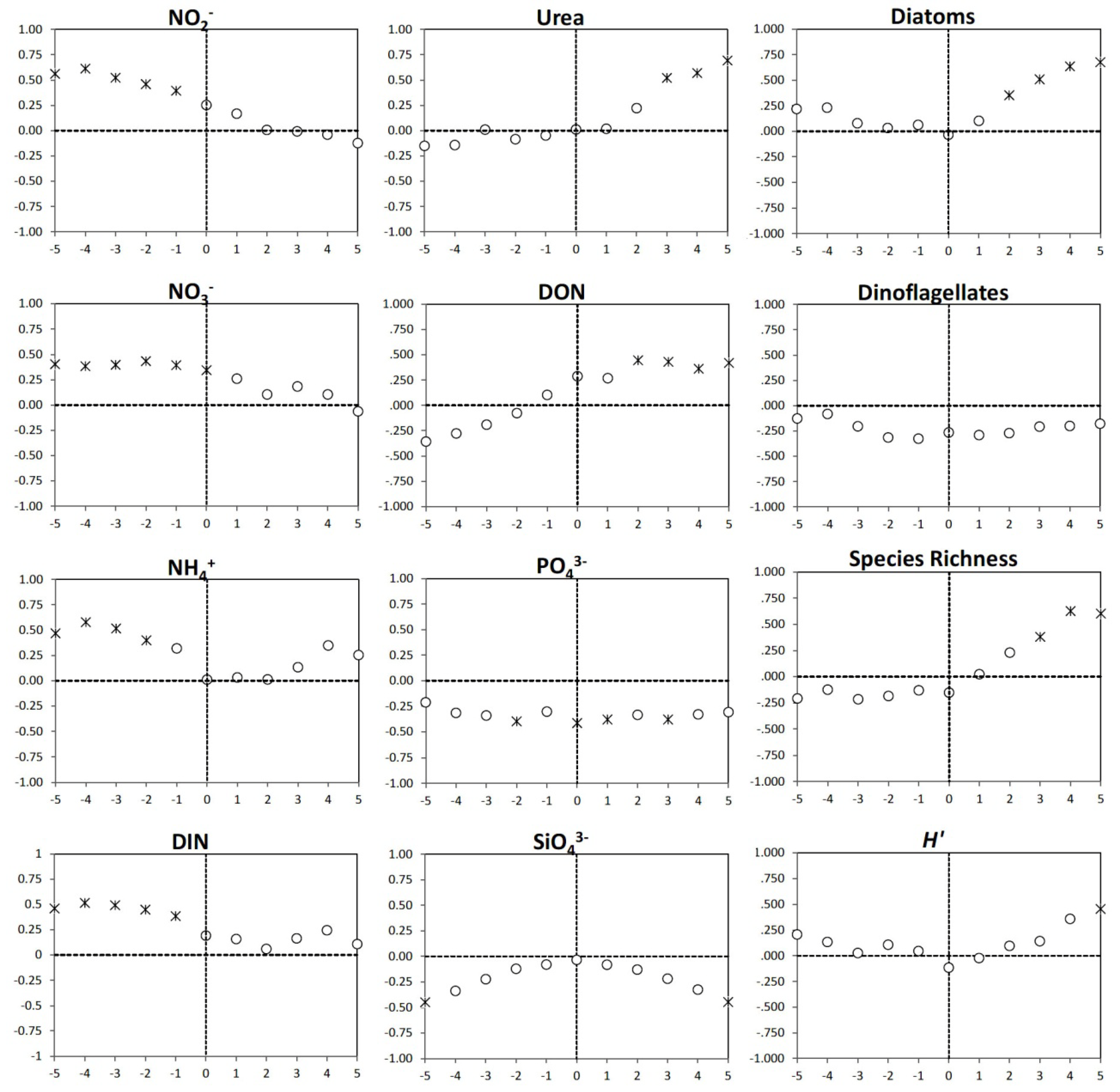
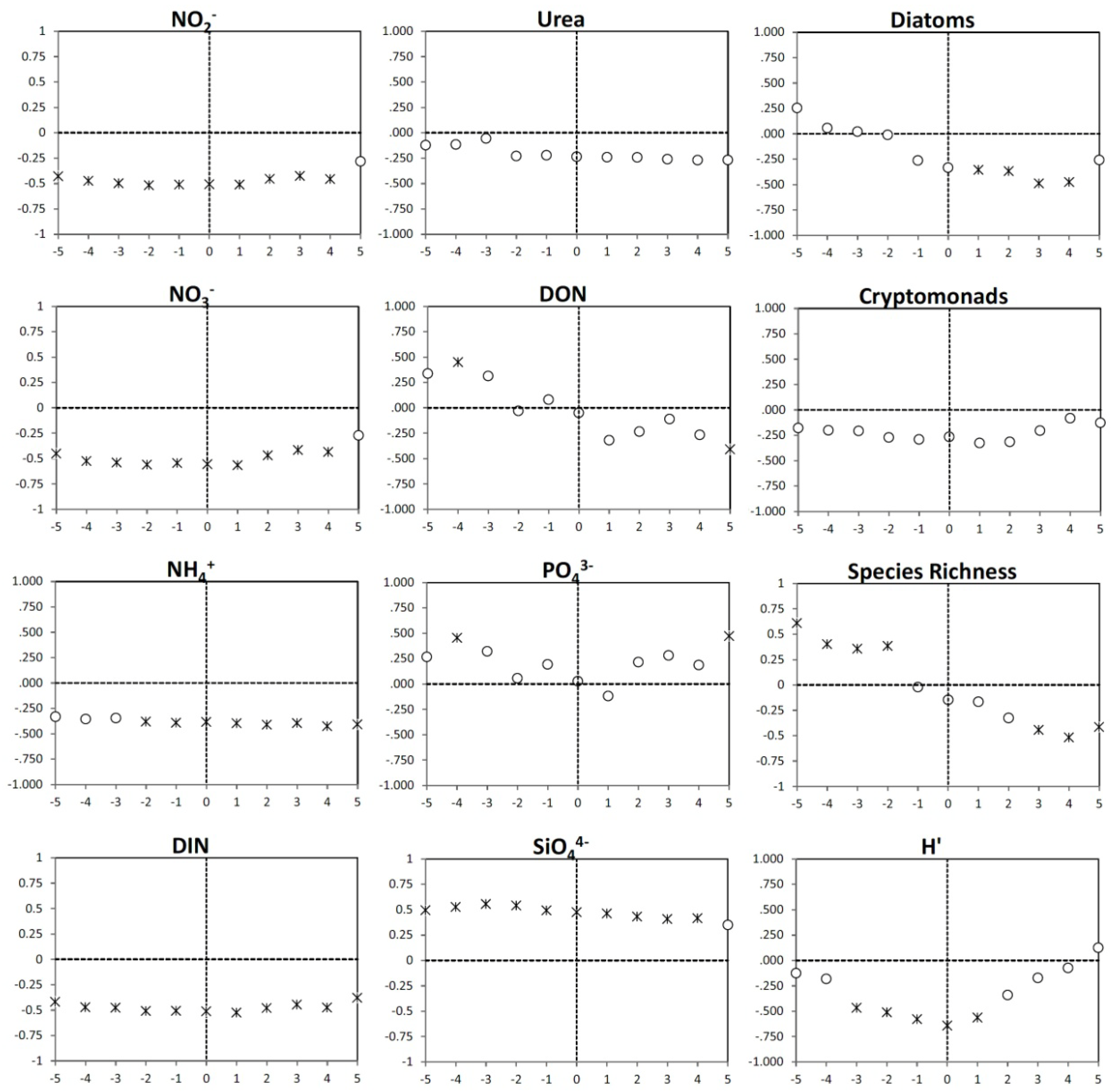
3.4. Time Lag Correlations

To understand the impact of environmental and biological conditions on the dominant phytoplankton in the community, time lagged correlations between cryptomonad and dinoflagellate abundances and individual nutrient concentrations and biological indicators were done. Significant positive correlations were observed between all forms of DIN and cryptomonad abundance 1 to 5 days later (Figure 7). These results suggest that with increases in DIN concentrations, cryptomonad populations respond by increasing their abundance. In contrast, the significant positive time lagged correlations between cryptomonad abundance and urea and DON concentrations indicate that urea and DON concentrations increased 2 to 5 days after cryptophyte abundance increased. This suggests that DON and urea were produced by or as a result of the cryptophyte bloom. There were negative correlations between PO43− and silicate concentrations and cryptomonad abundance both before and after the bloom. Cryptomonad abundance was also positively lag correlated with diatom abundance 2 to 5 days later, indicating that cryptomonad abundance might be related to the growth of diatoms, which could explain the negative correlation with silicate, albeit through an unknown mechanism Positive relationships between cryptomonad abundance and diversity were identified; significant correlations with species richness found 3 to 5 days after the bloom and H′ five days after the bloom (Figure 7).
Figure 7. Time lag Pearson correlation plots of cryptomonad abundance versus nutrient concentrations, diatom abundance, dinoflagellate abundance, phytoplankton species richness and diversity (Shannon index H′). Periods of plus or minus five days are shown on the X-axis with 0 being present. The Pearson correlation coefficient is plotted on the Y-axis, with positive values indicating positive relationships, and negative values negative relationships. Correlations that are statistically significant at the p < 0.05 level are indicated by asterisks.
Microorganisms 02 00033 g007
In contrast to the cryptomonads, dinoflagellates bloomed when DIN concentrations were at their lowest during the study period and as such, dinoflagellate abundance was negatively correlated with DIN concentrations, both in reverse and forward time (Figure 8). No significant correlations were found between urea concentrations and dinoflagellate abundance. Positive correlations between PO43− concentration and dinoflagellate abundance were identified, but significant only four days prior and five days after the bloom likely due to uptake by dinoflagellates during growth and regeneration after the bloom. Significant positive correlations were identified between silicate and dinoflagellate abundance, likely due to the fact that Si is not generally required for dinoflagellate growth and so was not being removed. Cryptomonad abundance and dinoflagellate abundance were negatively correlated, but not significantly (p < 0.05). Diatom abundance 1 to 4 days after the bloom was significantly negative correlated with dinoflagellate abundance; as dinoflagellate abundances decreased, diatom abundances increased. There were contrasting relationships identified between dinoflagellate abundance and diversity metrics. Dinoflagellate abundance was significantly positively correlated with species richness 2 to 5 days prior and negatively correlated 3 to 5 days after the bloom. Negative correlations between species diversity (H′) and dinoflagellate abundance were observed starting three days before the bloom and extending into the day after the bloom.
Figure 8. Time lag Pearson correlation plots of dinoflagellate abundance versus nutrient concentrations, diatom abundance, cryptomonad abundance, phytoplankton species richness and diversity (Shannon index H′). Periods of plus or minus five days are shown on the X-axis with 0 being present. The Pearson correlation coefficient is plotted on the Y-axis, with positive values indicating positive relationships, and negative values negative relationships. Correlations that are statistically significant at the p < 0.05 level are indicated by asterisks.
Microorganisms 02 00033 g008

3.5. Discussion

Fundamental to understanding the distribution and abundance of phytoplankton groups is their relationship to environmental variables that vary over short and long timescales in estuarine environments such as the Chesapeake Bay [49,50]. Estuaries are dynamic environments where chemical and physical parameters can vary over short time periods (e.g., tidal, sub-tidal, and diurnal), in response to episodic events such as storms (e.g., heavy rainfall and wind that impact salinity, temperature, stratification, turbidity, and nutrient concentrations), and over longer time scales due to climatic and anthropogenic forcing [21,51,52,53,54]. This study was aimed at understanding how environmental and biological factors combine to favor the formation of monospecific algal blooms over relatively short timescales during spring when rainfall and air and water temperatures can be highly variable resulting in short-term changes in salinity and nutrient concentrations in surface waters.
During the course of this 34-day study, two distinct blooms developed and dissipated, each over an approximately 7-day period. The first was a due to cryptomonad species common to the Lafayette River estuary, and the second a dinoflagellate, Gymnodinium instriatum. Neither bloom was detected during monthly monitoring of the estuary. Cryptomonads are a common component of estuarine phytoplankton communities throughout the year and comprise a major portion of the algal biomass in Virginia estuaries [55]. Their abundance has been associated with disturbances such as wind induced mixing of the water column and precipitation [44,56]. Cryptomonads are also readily preyed on by grazers that include ciliates, cladocerans, copepods, and dinoflagellates [44,57,58]. Gymnodinium instriatum (Freudenthal et Lee) Coats is an unarmored dinoflagellate that can form dense blooms, often producing “red tides” in coastal waters throughout the world, and has been associated with shellfish mortality through oxygen depletion [5,6,7,8,9,10,11,12,13,14,15,16,17,18,19,20,21,22,23,24,25,26,27,28,29,30,31,32,33,34,35,36,37,38,39,40,41,42,43,44,45,46,47,48,49,50,51,52,53,54,55,56,57,58,59,60]. G. instriatum is mixotrophic, and has been reported to feed on a variety of ciliates [61]. It is likely that it can also feed on cryptophytes, as has been observed for other mixotrophic dinoflagellates [62,63] G. instriatum, like many dinoflagellates is also capable of forming cysts when under environmental stress [64]. While this species has a wide salinity tolerance and is a common component of the phytoplankton community in tropical and temperate estuaries [46,47,48,49,50,51,52,53,54,55,56,57,58,59,60,61,62,63,64,65], its abundance in the Chesapeake Bay estuary is largely unknown due to its gross morphological similarity to a variety of other Gymnodinium and Gyrodinium dinoflagellates. It has been documented within the Bay using molecular techniques [47,66]; however, little is known about the conditions promoting blooms of G. instriatum in the environment [65].
Seasonal changes in water temperature and water quality affect species succession, the composition of plankton communities, and the particular organisms available to bloom seasonally [17,67,68,69]. During bloom initiation, the concentrations of particular algal species or assemblages within the planktonic community can change rapidly, often resulting in dominance by a single or a few species and reduced algal species diversity [4]. Monospecific blooms can develop and deteriorate over short time periods or may extend for months in estuarine systems [21,22].
One short-term forcing function that impacts physical and chemical conditions in temperate estuaries is storms and their associated wind and rainfall [52,70,71]. In shallow systems high winds can inject nutrients from the sediments as a result of intense mixing. In addition, rainfall can deliver nutrients directly through wet deposition or indirectly through overland and stream-flow. Inputs of freshwater can enhance stratification through the introduction of buoyancy. In many estuarine environments, wetlands and aquatic shoreline vegetation buffer the effects of seasonal or sporadic runoff by removing nutrients before they enter the estuary [72,73,74]. However, urban environments such as the Lafayette River, where the shoreline is highly developed and marsh covers less than half of its shoreline, storm water can enter the estuary directly through overland flow which is facilitated by impervious surfaces [29]. As a result, even relatively brief precipitation events can lead to large and rapid changes in water quality from storm sewer discharge and overland runoff [51,52,53,54,55,56,57,58,59,60,61,62,63,64,65,66,67,68,69,70,71,72,73,74,75].
Increases in Cryptomonas spp. cell density in the Lafayette River were first detected 48 h after a storm that delivered 0.74 cm of rain on 22 April. Cell densities reached their maximum about 48 h after a second rainfall of 2.8 cm on 25 April. The rainfall resulted in a decrease in surface salinity and increases in dissolved inorganic nitrogen concentrations, particularly NO3+ and NH4+. While the densities of Cryptomonas spp. increased rapidly, those of diatoms and other phytoplankton decreased. This resulted in a lower Shannon diversity index (H′). There was no corresponding decline in species richness, indicating the reduction in diversity was due to reduced species evenness. During the height of this bloom, Cryptomonas spp. dominated the phytoplankton community, comprising 91% of the algal biomass (Figure 2b). Based on daily changes in their abundance, the apparent net growth rate of Cryptomonas sp. during the period between 22 and 27 April was 0.86 divisions per day, similar to upper limits of Cryptomonas growth rates observed in cultures [76]. Because this estimate does not take into account potential losses due to grazing or advection, this rate should be considered a conservative one.
While ammonium concentrations increased after rainfall events, concentrations decreased concomitantly with increases in Cryptomonas abundance, suggesting its rapid uptake to support cellular growth. This is consistent with laboratory studies demonstrating high rates of ammonium uptake by Cryptomonas [77]. Within Chesapeake Bay, ammonium can be the dominant N form taken up by phytoplankton [78] and is often higher during summer as a result of N recycling [79]. Ammonium and nitrate levels increased again following rainfall on May 7–8. Again, ammonium concentrations declined more rapidly than nitrate, and this coincided with another peak in Cryptomonas abundance. DIN concentrations and Cryptomonas abundance were positively related in the lag-correlation analyses at periods of 1–5 days (Figure 7) suggesting that nutrient inputs from runoff may have stimulated Cryptomonas growth.
Gymnodinium instriatum was present at low cell densities (<100 cells mL−1) for the first 25 days of the study. However, about 48 h following the rainfall on May 14 and 15, G. instriatum populations burgeoned to over 30,000 cells mL−1, an apparent net growth rate of 3.3 divisions per day. This was over four times greater than the maximum growth rate reported for this species in laboratory cultures [65] but again did not account for grazing and advection losses or the effects of dinoflagellate swarming and aggregation [80]. A synchronous excystment of benthic dinocysts from river sediment may also have contributed to this rapid increase in G. instriatum abundance. Shikata et al. [64] (2008) showed that G. instriatum can excyst over a short period of time (≤3 days) at water temperatures ≥20 °C, consistent with those present during the time this bloom initiated.
Dinoflagellate cyst-beds are produced by several estuarine dinoflagellate species, and are thought to serve as a survival mechanism for organisms living in habitats where environmental conditions fluctuate [81,82]. Cyst formation in G. instriatum has been attributed to N and P limitation [64] and high cell densities [61]. High densities of a variety of benthic dinoflagellate cysts have been identified in tributaries of the lower Chesapeake Bay, including the Elizabeth and Lafayette Rivers [39,81]. Increases in summertime blooms of the pelagic dinoflagellate Cochlodinium polykrikoides in the Lafayette River and elsewhere in the lower Chesapeake Bay estuary have also been attributed to local cyst-beds [83,84]. Excystment of C. polykrikoides appears to be triggered by following summer rainfall events when water temperatures are ≥26 °C, likely due to nutrient inputs and enhanced stratification [7,21,22]. Water temperatures just prior to the rainfall May 14 and 15 had reached 22.6 °C. Following rainfall and during the subsequent G. instriatum bloom, DIN concentrations were near or below the analytical detection limit, likely because it was rapidly taken up by the emerging and rapidly growing dinoflagellates and so never accumulated in the environment.
While excystment and population growth of G. instriatum may be stimulated by runoff of nutrients into the river, this is not strongly supported by the lag correlation analysis. Instead, the opposite pattern was observed, with DIN concentrations negatively correlated with dinoflagellate abundance. Many harmful algal bloom taxa, including dinoflagellates, occur during periods when nutrients, particularly DIN, are depleted [17,21,22,85]. These conditions are thought to favor blooms of mixotrophic dinoflagellates over other taxa such as diatoms and cryptophytes that are more autotrophic [85]. Many dinoflagellates can use dissolved organic N (DON) and graze on co-occurring microbes including cryptophytes and unicellular cyanobacteria to augment their nutrition [86,87].
The G. instriatum bloom appeared to initiate after a spring storm and in addition to the associated nutrient loading, freshwater inputs also enhance stratification which can lead to rapid increases in dinoflagellate abundance relative to diatoms, including through excystment [21,88,89,90]. Alternatively, the high apparent net growth rate observed at the sampling location may be attributed to advection and transport of cells from elsewhere in the estuary. Collections were made at the same tidal period to reduce the impact of cyclical tidal advection on the observations, however freshwater input related flushing still would have an effect on transporting water mass and the plankton therein. Algal blooms are spatially heterogeneous and patchy, and it is possible that a bloom had developed upstream in response to nitrogen loading elsewhere, before being transported downstream through flushing. In this scenario, the dinoflagellate bloom may also have been directly related to increased nutrient inputs upstream, with depleted DIN concentrations occurring during transport before the bloom was sampled at the study site [91]. Uncertainty related to the origin of the bloom is an inherent property of a study of a dynamic water body with limited spatial coverage.
Additionally, species interactions, such as the abundance of potential algal prey, could have stimulated G. instriatum growth as have been shown for other mixotrophic dinoflagellates. Toxic Karlodinium veneficum blooms have been correlated with increases in cryptophyte abundance through the stimulation of grazing [58]. While grazing by G. instriatum was not measured in this study, Cryptomonas sp. abundances decreased as G. instriatum concentrations increased, and cryptophyte concentrations were the lowest during the dinoflagellate bloom (Figure 4b); however, cryptomonad and dinoflagellate abundance were not significantly correlated (Figure 7 and Figure 8).
Algal diversity (H′) was greatly reduced during both blooms, primarily due to decreased species evenness. This led to the significant negative correlation between species diversity and algal biomass (Figure 5a). Examination of diversity/productivity relationships in both terrestrial and aquatic systems have identified positive, negative and unimodal associations [41,92]. Similar studies of phytoplankton communities are more limited; however it appears that at a large enough productivity gradient, the relationship appears to be unimodal, with maximum diversity at intermediate phytoplankton biomass concentrations [93]. Surprisingly, while species diversity was low during blooms due to low evenness, phytoplankton species richness remained relatively high during blooms suggesting community resilience.
The phytoplankton abundances observed in this study were as much as an order of magnitude greater than those observed at Chesapeake Bay Program monthly monitoring stations in the polyhaline lower Chesapeake Bay watershed at the same time period [94]. Phytoplankton abundances observed during this study during the incoming tide (about 2 h after low tide) at our shallow-water station in the Lafayette River (5.7 × 10⁶–7.8 × 10⁷ cells L−1) were higher than those recorded at monthly monitoring stations occupied as part of the Virginia Chesapeake Bay Monitoring Program (CBMP) (1.8 × 10⁶–1.3 × 10⁷ cells L−1) during the same time period [94]. This highlights the unlikelihood of capturing blooms during monthly monitoring and the need for developing different tools for assessing these ephemeral events so that we can begin to understand causal factors promoting blooms in the environment.

4. Conclusions

Dinoflagellate blooms, appear to be increasing in magnitude and frequency in Chesapeake Bay and its tributaries and this has been linked to nutrient loading and eutrophication [20,23,34,95]. We examined the effects of water quality on phytoplankton community composition in an urban estuarine tributary susceptible to storm water input and seasonal dinoflagellate blooms. Blooms are ephemeral in nature and can develop rapidly in response to environmental forcing and so are undersampled by routine monthly monitoring programs. During this study, blooms of Cryptomonas sp. and G. instriatum developed and dispersed over short periods (5–7 days) of time between storms. Blooms were associated with reduced algal diversity but species richness remained relatively constant during the blooms. The rapid development and brief duration of both blooms emphasizes the importance of monitoring on appropriate temporal scales. The study also illustrates the compromises that are required when designing a monitoring experiment, as increased spatial coverage of the tributary may have helped explain bloom initiation and advection, but at the expense of temporal periodicity. These results build on a growing number of studies that indicate bloom emergence is complex, with water quality parameters (e.g., nutrient loading), hydrologic transport, and species interactions all contributing to bloom formation by mixotrophic taxa.

Acknowledgments

This research was supported in part by Virginia Department of Environmental Quality and the Chesapeake Bay Monitoring Program (HGM) and the Virginia Environmental Endowment and the National Science Foundation (MRM). The authors would like to thank Peter Bernhardt and Katherine Filippino and the members of the Phytoplankton Analysis Laboratory including Matthew Semcheski and Matthew Muller for their assistance.

Conflicts of Interest

The authors declare no conflict of interest.

References

  1. Hutchinson, G.E. The paradox of the plankton. Am. Nat. 1961, 95, 137–145. [Google Scholar]
  2. Grover, J.P.; Chrzanowski, T.H. Limiting resources, disturbance, and diversity in phytoplankton communities. Ecol. Monogr. 2004, 74, 533–551. [Google Scholar] [CrossRef]
  3. Cloern, J.E.; Dufford, R. Phytoplankton community ecology: Principles applied in San Francisco Bay. Mar. Ecol. Prog. Ser. 2005, 285, 11–28. [Google Scholar] [CrossRef]
  4. Spatharis, S.; Tsirtsis, G.; Danielidis, D.B.; Chi, T.D.; Mouillot, D. Effects of pulsed nutrient inputs on phytoplankton assemblage structure and blooms in an enclosed coastal area. Estuar. Coast. Shelf Sci. 2007, 73, 807–815. [Google Scholar] [CrossRef]
  5. Hubertz, E.D.; Cahoon, L.B. Short-term variability of water quality parameters in two shallow estuaries of North Carolina. Estuaries 1999, 22, 814–823. [Google Scholar] [CrossRef]
  6. Filippino, K.C.; Egerton, T.A.; Morse, R.E.; Hunley, W.S.; Mulholland, M.R. Nutrient dynamics in the tidal James River before, during, and after Hurricane Irene and Tropical Storm Lee. Estuar. Coast. Shelf Sci. 2013. submitted for publication. [Google Scholar]
  7. Morse, R.E.; Mulholland, M.R.; Egerton, T.A.; Marshall, H.G. Daily variability in phytoplankton abundance and nutrient concentrations in a tidally dominated eutrophic estuary. Mar. Ecol. Prog. Ser. 2013. submitted for publication. [Google Scholar]
  8. Morse, R.E.; Mulholland, M.R.; Hunley, W.S.; Fentress, S.; Wiggins, M.; Blanco-Garcia, J.L. Controls on the initiation and development of blooms of the dinoflagellate Cochlodinium polykrikoides Margalef in lower Chesapeake Bay and its tributaries. Harmful Algae 2013, 28, 71–82. [Google Scholar] [CrossRef]
  9. McCormick, P.V.; Cairns, J., Jr. Algae as indicators of environmental change. J. Appl. Phycol. 1994, 6, 509–526. [Google Scholar] [CrossRef]
  10. Buchanan, C.; Lacouture, R.V.; Marshall, H.G.; Olson, M.; Johnson, J.M. Phytoplankton reference communities for Chesapeake Bay and its tidal tributaries. Estuaries 2005, 28, 138–159. [Google Scholar] [CrossRef]
  11. Paerl, H.W.; Valdes-Weaver, L.M.; Joyner, A.R.; Winkelmann, V. Phytoplankton indicators of ecological change in the eutrophying Pamlico Sound system, North Carolina. Ecol. Appl. 2007, 17, S88–S101. [Google Scholar] [CrossRef]
  12. Litaker, W.; Duke, C.S.; Kenny, B.E.; Ramus, J. Short-term environmental variability and phytoplankton abundance in a shallow tidal estuary. II. Spring and fall. Mar. Ecol. Prog. Ser. 1993, 94, 141–154. [Google Scholar] [CrossRef]
  13. Malone, T.C.; Conley, D.J.; Fisher, T.R.; Glibert, P.M.; Harding, L.W.; Sellner, K.G. Scales of nutrient-limited phytoplankton productivity in Chesapeake Bay. Estuaries 1996, 19, 371–385. [Google Scholar] [CrossRef]
  14. Paerl, H.W.; Rossignol, K.L.; Hall, S.N.; Peierls, B.L.; Wetz, M.S. Phytoplankton community indicators of short-and long-term ecological change in the anthropogenically and climatically impacted Neuse River Estuary, North Carolina, USA. Estuar. Coasts 2010, 33, 485–497. [Google Scholar] [CrossRef]
  15. Duarte, P.; Macedo, M.F.; da Fonseca, L.C. The relationship between phytoplankton diversity and community function in a coastal lagoon. Hydrobiologia 2006, 555, 3–18. [Google Scholar] [CrossRef]
  16. Jouenne, F.; Lefebvre, S.; Véron, B.; Lagadeuc, Y. Phytoplankton community structure and primary production in small intertidal estuarine-bay ecosystem (eastern English Channel, France). Mar. Biol. 2007, 151, 805–825. [Google Scholar] [CrossRef]
  17. Glibert, P.M.; Magnien, R.; Lomas, M.W.; Alexander, J.; Tan, C.; Haramoto, E.; Trice, M.; Kana, T.M. Harmful algal blooms in the Chesapeake and coastal bays of Maryland, USA: Comparison of 1997, 1998, and 1999 events. Estuaries 2001, 24, 875–883. [Google Scholar] [CrossRef]
  18. Gobler, C.J.; Burson, A.; Koch, F.; Tang, Y.; Mulholland, M.R. The role of nitrogenous nutrients in the occurrence of harmful algal blooms caused by Cochlodinium polykrikoides in New York estuaries (USA). Harmful Algae 2012, 17, 64–74. [Google Scholar] [CrossRef]
  19. Anderson, D.M.; Glibert, P.M.; Burkholder, J.M. Harmful algal blooms and eutrophication: Nutrient sources, composition, and consequences. Estuaries 2002, 25, 704–726. [Google Scholar] [CrossRef]
  20. Heisler, J.; Glibert, P.M.; Burkholder, J.M.; Anderson, D.M.; Cochlan, W.; Dennison, W.C.; Dortch, Q.; Gobler, C.J.; Heil, C.A.; Humphries, E.; et al. Eutrophication and harmful algal blooms: A scientific consensus. Harmful Algae 2008, 8, 3–13. [Google Scholar] [CrossRef]
  21. Morse, R.E.; Shen, J.; Blanco-Garcia, J.L.; Hunley, W.S.; Fentress, S.; Wiggins, M.; Mulholland, M.R. Environmental and physical controls on the formation and transport of blooms of the dinoflagellate Cochlodinium polykrikoides Margalef in the lower Chesapeake Bay and its tributaries. Estuar. Coasts 2011, 34, 1006–1025. [Google Scholar] [CrossRef]
  22. Mulholland, M.R.; Morse, R.E.; Boneillo, G.E.; Bernhardt, P.W.; Filippino, K.C.; Procise, L.A.; Blanco-Garcia, J.L.; Marshall, H.G.; Egerton, T.A.; Hunley, W.S.; et al. Understanding causes and impacts of the dinoflagellate, Cochlodinium polykrikoides, blooms in the Chesapeake Bay. Estuar. Coasts 2009, 32, 734–747. [Google Scholar] [CrossRef]
  23. Mulholland, M.R.; Boneillo, G.E.; Bernhardt, P.W.; Minor, E.C. Comparison of nutrient and microbial dynamics over a seasonal cycle in a mid-Atlantic coastal lagoon prone to Aureococcus anophagefferens (brown tide) blooms. Estuar. Coasts 2009, 32, 1176–1194. [Google Scholar] [CrossRef]
  24. Glibert, P.M.; Kelly, V.; Alexander, J.; Codispoti, L.A.; Boicourt, W.C.; Trice, T.M.; Michael, B. In situ nutrient monitoring: A tool for capturing nutrient variability and the antecedent conditions that support algal blooms. Harmful Algae 2008, 8, 175–181. [Google Scholar] [CrossRef]
  25. Mitchell-Innes, B.A.; Walker, D.R. Short-term variability during an anchor station study in the southern Benguela upwelling system: Phytoplankton production and biomass in relation to specie changes. Prog. Oceanogr. 1991, 28, 65–89. [Google Scholar] [CrossRef]
  26. Blair, C.H.; Cox, J.H.; Kuo, C.Y. Investigation of Flushing Time in the Lafayette River, Norfolk, Virginia; School of Engineering Technical Report No. 76-C4; Old Dominion University: Norfolk, VA, USA, 1976. [Google Scholar]
  27. White, E.G. A Physical Hydrographic Study of the Lafayette River. M.S. Thesis, Old Dominion University, Norfolk, VA, USA, 1972. [Google Scholar]
  28. Owen, D.W.; Rogers, L.M.; Peoples, M.H. Shoreline Situation Report; Cities of Chesapeake, Norfolk, and Portsmouth; Special Report in Applied Marine Science and Oceanic Engineering Number 136; Virginia Institute of Marine Science: Gloucester Point, VA, USA, 1976. [Google Scholar]
  29. Berman, M.; Berquist, H.; Hershner, C.; Killeen, S.; Rudnicky, T.; Schatt, D.; Weiss, D.; Woods, H. City of Norfolk Shoreline Situation Report; Special Report in Applied Marine Science and Ocean Engineering Number 378; Virginia Institute of Marine Science: Gloucester Point, VA, USA, 2002. [Google Scholar]
  30. Purcell, T.W. Phytoplankton Succession in the Lafayette River Estuary, Norfolk, Virginia. M.S. Thesis, Old Dominion University, Norfolk, VA, USA, 1973. [Google Scholar]
  31. Marshall, H.G. Plankton in James River Estuary, Virginia III. Phytoplankton in the Lafayette and Elizabeth Rivers (Western and Eastern Branches). Castanea 1968, 33, 255–258. [Google Scholar]
  32. Kalenak, L.A. Factors Effecting Phytoplankton Assemblages in the Lafayette River Estuary. M.S. Thesis, Old Dominion University, Norfolk, Virginia, USA, 1982. [Google Scholar]
  33. Egerton, T.A.; Marshall, H.G.; Hunley, W.S. Integration of Microscopy and Underway Chlorophyll Mapping for Monitoring Algal Bloom Development. Oceans 2012, 2012. [Google Scholar] [CrossRef]
  34. Welschmeyer, N.A. Fluorometric analysis of chlorophyll a in the presence of chlorophyll b and pheopigments. Limnol. Oceanogr. 1994, 39, 1985–1992. [Google Scholar] [CrossRef]
  35. Solarzano, L. Determination of ammonia in natural waters by the phenol hypochlorite method. Limnol. Oceanogr. 1969, 14, 16–23. [Google Scholar] [CrossRef]
  36. Marshall, H.G.; Alden, R.W. A comparison of phytoplankton assemblages and environmental relationships in three estuarine rivers of the lower Chesapeake Bay. Estuaries 1990, 13, 287–300. [Google Scholar] [CrossRef]
  37. Affronti, L.F.; Marshall, H.G. Using frequency of dividing cells in estimating autotrophic picoplankton growth and productivity in the Chesapeake Bay. Hydrobiologia 1994, 284, 193–203. [Google Scholar] [CrossRef]
  38. Smayda, T.J. From Phytoplankters to Biomass. In Phytoplankton Manual; UNESCO: Paris, France, 1978; pp. 273–279. [Google Scholar]
  39. Tang, Y.Z.; Egerton, T.A.; Kong, L.; Marshall, H.G. Morphological variation and phylogenetic analysis of the dinoflagellate Gymnodinium aureolum from a tributary of Chesapeake Bay. J. Eukaryot. Microbiol. 2008, 55, 91–99. [Google Scholar] [CrossRef]
  40. Shannon, C.; Weaver, W. The Mathematical Theory Information; University of Illinois Press: Urbana, IL, USA, 1949. [Google Scholar]
  41. Waide, R.B.; Willig, M.R.; Steiner, C.F.; Mittelbach, G.; Gough, L.; Dodson, S.I.; Juday, P.; Parmenter, R. The relationship between productivity and species richness. Annu. Rev. Ecol. Syst. 1999, 30, 257–300. [Google Scholar]
  42. Quinn, G.P.; Keough, M.J. Experimental Design and Data Analysis for Biologists; Cambridge University Press: Cambridge, UK, 2002. [Google Scholar]
  43. Witman, J.D.; Cusson, M.; Archambault, P.; Pershing, A.J.; Mieszkowska, N. The relation between productivity and species diversity in temperate-arctic marine ecosystems. Ecology 2008, 89, S66–S80. [Google Scholar] [CrossRef]
  44. Klaveness, D. Ecology of the Cryptomonadida: A First Review. In Growth and Reproductive Strategies of Freshwater Phytoplankton; Sandgren, C.D., Ed.; Cambridge University Press: Cambridge, UK, 1988; pp. 105–134. [Google Scholar]
  45. Menezes, M.; Novarino, G. How diverse are planktonic cryptomonads in Brazil? Advantages and difficulties of a taxonomic-biogeographical approach. Hydrobiologia 2003, 502, 297–306. [Google Scholar] [CrossRef]
  46. Steidinger, K.A.; Tangen, K. Dinoflagellates. In Identifying Marine Phytoplankton; Tomas, C.R., Ed.; Academic Press: San Diego, CA, USA, 1997; pp. 387–598. [Google Scholar]
  47. Coats, D.W.; Park, M.G. Parasitism of photosynthetic dinoflagellates by three strains of Amoebophrya (Dinophyta): Parasite survival, infectivity, generation time, and host specificity. J. Phycol. 2002, 38, 520–528. [Google Scholar]
  48. Conley, D.J.; Malone, T.C. Annual cycle of dissolved silicate in Chesapeake Bay: Implications for the production and fate of phytoplankton biomass. Mar. Ecol. Prog. Ser. 1992, 81, 121–128. [Google Scholar] [CrossRef]
  49. Marshall, H.G.; Lane, M.F.; Nesius, K.K.; Burchardt, L. Assessment and significance of phytoplankton species composition within Chesapeake Bay and Virginia tributaries through a long-term monitoring program. Environ. Monit. Assess. 2009, 150, 143–155. [Google Scholar] [CrossRef]
  50. Williams, M.R.; Filoso, S.; Longstaff, B.J.; Dennison, W.C. Long-term trends of water quality and biotic metrics in Chesapeake Bay: 1986 to 2008. Estuar. Coasts 2010, 33, 1279–1299. [Google Scholar] [CrossRef]
  51. Roberts, D.A.; Poore, A.G.; Johnston, E.L. MBACI sampling of an episodic disturbance: Storm water effects on algal epifauna. Mar. Environ. Res. 2007, 64, 514–523. [Google Scholar] [CrossRef]
  52. Najjar, R.G.; Pyke, C.R.; Adams, M.B.; Breitburg, D.; Hershner, C.; Kemp, M.; Howarth, R.; Mulhollad, M.R.; Paolisso, M.; Secor, D.; et al. Potential climate-change impacts on the Chesapeake Bay. Estuar. Coast. Shelf Sci. 2010, 86, 1–20. [Google Scholar] [CrossRef]
  53. Orth, R.J.; Williams, M.R.; Marion, S.R.; Wilcox, D.J.; Carruthers, T.J.; Moore, K.A.; Kemp, W.M.; Dennison, W.C.; Rybicki, N.; Bergstrom, P.; et al. Long-term trends in submersed aquatic vegetation (SAV) in Chesapeake Bay, USA, related to water quality. Estuar. Coasts 2010, 33, 1144–1163. [Google Scholar] [CrossRef]
  54. Cho, K.H.; Wang, H.V.; Shen, J.; Valle-Levinson, A.; Teng, Y.C. A modeling study on the response of Chesapeake Bay to hurricane events of Floyd and Isabel. Ocean Model. 2012, 49, 22–46. [Google Scholar]
  55. Marshall, H.G.; Lacouture, R.V.; Buchanan, C.; Johnson, J.M. Phytoplankton assemblages associated with water quality and salinity regions in Chesapeake Bay, USA. Estuar. Coast. Shelf Sci. 2006, 69, 10–18. [Google Scholar] [CrossRef]
  56. Mallin, M.A.; Paerl, H.W.; Rudek, J. Seasonal phytoplankton composition, productivity and biomass in the Neuse River estuary, North Carolina. Estuar. Coast. Shelf Sci. 1991, 32, 609–623. [Google Scholar] [CrossRef]
  57. Weisse, T.; Kirchhoff, B. Feeding of the heterotrophic freshwater dinoflagellate. Peridiniopsis berolinense on cryptophytes: Analysis by flow cytometry and electronic particle counting. Aquat. Microb. Ecol. 1997, 12, 153–164. [Google Scholar] [CrossRef]
  58. Adolf, J.E.; Bachvaroff, T.; Place, A.R. Can cryptophyte abundance trigger toxic Karlodinium veneficum blooms in eutrophic estuaries? Harmful Algae 2008, 8, 119–128. [Google Scholar] [CrossRef]
  59. Jimenéz, R. Ecological Factors Related to Gyrodinium instriatum Bloom in the Inner Estuary of the Gulf of Guayaquil. In Toxic Phytoplankton Blooms in the Sea; Smayda, T.J., Shimizu, Y., Eds.; Elsevier: Amsterdam, The Netherlands, 1993; pp. 257–262. [Google Scholar]
  60. Kim, H.G.; Park, J.S.; Lee, S.G.; An, K.H. Population Cell Volume and Carbon Content in Monospecific Dinoflagellate Blooms. In Toxic Phytoplankton Blooms in the Sea; Smayda, T.J., Shimizu, Y., Eds.; Elsevier: Amsterdam, The Netherlands, 1993; pp. 769–773. [Google Scholar]
  61. Uchida, T.; Kamiyama, T.; Matsuyama, Y. Predation by a photosynthetic dinoflagellate Gyrodinium instriatum on loricated ciliates. J. Plankton Res. 1997, 19, 603–608. [Google Scholar] [CrossRef]
  62. Li, A.; Stoecker, D.K.; Coats, D.W. Use of the ‘food vacuole content’ method to estimate grazing by the mixotrophic dinoflagellate Gyrodinium galatheanum on cryptophytes. J. Plankton Res. 2001, 23, 303–318. [Google Scholar] [CrossRef]
  63. Hansen, P.J. The role of photosynthesis and food uptake for the growth of marine mixotrophic dinoflagellates1. J. Eukaryot. Microbiol. 2001, 58, 203–214. [Google Scholar] [CrossRef]
  64. Shikata, T.; Nagasoe, S.; Matsubara, T.; Yamasaki, Y.; Shimasaki, Y.; Oshima, Y.; Uchida, T.; Jenkinson, I.R.; Honjo, T. Encystment and excystment of Gyrodinium instriatum Freudenthal et Lee. J. Oceanogr. 2008, 64, 355–365. [Google Scholar] [CrossRef]
  65. Nagasoe, S.; Kim, D.I.; Shimasaki, Y.; Oshima, Y.; Yamaguchi, M.; Honjo, T. Effects of temperature, salinity and irradiance on the growth of the red tide dinoflagellate Gyrodinium instriatum Freudenthal et Lee. Harmful Algae 2006, 5, 20–25. [Google Scholar] [CrossRef]
  66. Malmquist, D. VIMS researchers monitor harmful algal bloom. Available online: http://www.vims.edu/newsandevents/topstories/alexandrium_bloom.php (accessed on 20 April 2013).
  67. Marshall, H.G. Seasonal phytoplankton composition in the lower Chesapeake Bay and Old Plantation Creek, Cape Charles, Virginia. Estuaries 1980, 3, 207–216. [Google Scholar] [CrossRef]
  68. Marshall, H.G.; Lacouture, R. Seasonal patterns of growth and composition of phytoplankton in the lower Chesapeake Bay and vicinity. Estuar. Coast. Shelf Sci. 1986, 23, 115–130. [Google Scholar] [CrossRef]
  69. Adolf, J.E.; Yeager, C.L.; Miller, W.D.; Mallonee, M.E.; Harding, L.W. Environmental forcing of phytoplankton floral composition, biomass, and primary productivity in Chesapeake Bay, USA. Estuar. Coast. Shelf Sci. 2006, 67, 108–122. [Google Scholar] [CrossRef]
  70. Jordan, T.E.; Correll, D.L.; Weller, D.E. Relating nutrient discharges from watersheds to land use and stream flow variability. Water Resour. Res. 1997, 33, 2579–2590. [Google Scholar] [CrossRef]
  71. Langland, M.J.; Phillips, S.W.; Raffensperger, J.P.; Moyer, D.L. Changes in Stream Flow and Water Quality in Selected Nontidal Sites in the Chesapeake Bay Basin, 1985–2003; U.S. Geological Survey Scientific Investigations Report 2004–5259; U.S. Geological Survey: Baltimore, MD, USA, 2004; p. 50. [Google Scholar]
  72. Vought, L.B.M.; Pinay, G.; Fuglsang, A.; Ruffinoni, C. Structure and function of buffer strips from a water quality perspective in agricultural landscapes. Landsc. Urban Plan. 1995, 31, 323–331. [Google Scholar] [CrossRef]
  73. Laws, E.A.; Ziemann, D.; Schulman, D. Coastal water quality in Hawaii: The importance of buffer zones and dilution. Mar. Environ. Res. 1999, 48, 1–21. [Google Scholar] [CrossRef]
  74. Syversen, N.; Haarstad, K. Retention of pesticides and nutrients in a vegetated buffer root zone compared to soil with low biological activity. Int. J. Environ. Anal. Chem. 2005, 85, 1175–1187. [Google Scholar] [CrossRef]
  75. Nichols, F.H.; Cloern, J.E.; Luoma, S.N.; Peterson, D.H. The modification of an estuary. Science 1986, 231, 567–573. [Google Scholar]
  76. Sciandra, A.; Lazzara, L.; Claustre, H.; Babin, M. Responses of growth rate, pigment composition and optical properties of Cryptomonas sp. to light and nitrogen stresses. Mar. Ecol. Prog. Ser. 2000, 201, 107–120. [Google Scholar] [CrossRef]
  77. Cloern, J.E. Effects of light intensity and temperature on Cryptomonas ovata (Cryptophyceae) growth and nutrient uptake rates. J. Phycol. 1977, 13, 389–395. [Google Scholar]
  78. Bradley, P.B.; Lomas, M.W.; Bronk, D.A. Inorganic and organic nitrogen use by phytoplankton along Chesapeake Bay, measured using a flow cytometric sorting approach. Estuar. Coasts 2010, 33, 971–984. [Google Scholar] [CrossRef]
  79. Kemp, W.M.; Boynton, W.R.; Adolf, J.E.; Boesch, D.F.; Boicourt, W.C.; Brush, G.; Cornwell, J.C.; Fisher, T.R.; Glibert, P.M.; Hagy, J.D.; et al. Eutrophication of Chesapeake Bay: Historical trends and ecological interactions. Mar. Ecol. Prog. Ser. 2005, 303, 1–29. [Google Scholar] [CrossRef]
  80. Furnas, M.J. In situ growth rates of marine phytoplankton: Approaches to measurement, community and species growth rates. J. Plankton Res. 1990, 12, 1117–1151. [Google Scholar] [CrossRef]
  81. Anderson, D.M.; Wall, D. Potential importance of benthic cysts of Gonyaulax tamarensis and G. excavates in initiating toxic dinoflagellate blooms. J. Phycol. 1978, 20, 224–234. [Google Scholar] [CrossRef]
  82. Anderson, D.M.; Rengefors, K. Community assembly and seasonal succession of marine dinoflagellates in a temperate estuary: The importance of life cycle events. Limnol. Oceanogr. 2006, 51, 860–873. [Google Scholar] [CrossRef]
  83. Seaborn, D.W.; Marshall, H.G. Dinoflagellate cysts within sediment collections from the southern Chesapeake Bay and tidal regions of the James, York, and Rappahannock rivers. Va. J. Sci. 2008, 59, 135–141. [Google Scholar]
  84. Tomas, C.R.; Smayda, T.J. Red tide blooms of Cochlodinium polykrikoides in a coastal cove. Harmful Algae 2008, 7, 308–317. [Google Scholar] [CrossRef]
  85. Sunda, W.G.; Graneli, E.; Gobler, C.J. Positive feedback and the development and persistence of ecosystem disruptive algal blooms. J. Phycol. 2006, 42, 963–974. [Google Scholar] [CrossRef]
  86. Berman, T.; Bronk, D.A. Dissolved organic nitrogen: A dynamic participant in aquatic ecosystems. Aquat. Microb. Ecol. 2003, 31, 279–305. [Google Scholar] [CrossRef]
  87. Li, A.; Stoecker, D.K.; Coats, D.W. Spatial and temporal aspects of Gyrodinium galatheanum in Chesapeake Bay: Distribution and mixotrophy. J. Plankton Res. 2000, 22, 2105–2124. [Google Scholar] [CrossRef]
  88. Tyler, M.A.; Seliger, H.H. Annual subsurface transport of a red tide dinoflagellate to its bloom area: Water circulation patterns and organism distributions in the Chesapeake Bay. Limnol. Oceanogr. 1978, 23, 227–246. [Google Scholar] [CrossRef]
  89. Nehring, S. Mechanisms for Recurrent Nuisance Algal Blooms in Coastal Zones: Resting Cyst Formation as Life-Strategy of Dinoflagellates. In Proceedings of the International Coastal Congress, ICC-Kiel 92: Interdisciplinary Discussion of Coastal Research and Coastal Management Issues and Problems; Sterr, H., Hofstade, J., Plag, H.-P., Eds.; P. Lang: Frankfurt, Germany, 1993; pp. 454–467. [Google Scholar]
  90. Sellner, K.G.; Sellner, S.G.; Lacouture, R.V.; Magnien, R.E. Excessive nutrients select for dinoflagellates in the stratified Patapsco River estuary: Margalef reigns. Mar. Ecol. Prog. Ser. 2001, 220, 93–102. [Google Scholar] [CrossRef]
  91. Peierls, B.L.; Hall, N.S.; Paerl, H.W. Non-monotonic responses of phytoplankton biomass accumulation to hydrologic variability: A comparison of two coastal plain North Carolina estuaries. Estuar. Coasts 2012, 35, 1376–1392. [Google Scholar] [CrossRef]
  92. Leibold, M.A. Biodiversity and nutrient enrichment in pond plankton communities. Evolut. Ecol. Res. 1999, 1, 73–95. [Google Scholar]
  93. Irigoien, X.; Huisman, J.; Harris, R.P. Global biodiversity patterns of marine phytoplankton and zooplankton. Nature 2004, 429, 863–867. [Google Scholar] [CrossRef]
  94. Chesapeake Bay Program Plankton Database. Available online: http://www.chesapeakebay.net/data/downloads/baywide_cbp_plankton_database (accessed on 20 April 2013).
  95. Glibert, P.M.; Alexander, J.; Meritt, D.W.; North, E.W.; Stoecker, D.K. Harmful algae pose additional challenges for oyster restoration: Impacts of the harmful algae Karlodinium veneficum, and Prorocentrum minimum on early life stages of the oysters Crassostrea virginica and Crassostrea ariakensis. J. Shellfish Res. 2007, 26, 919–925. [Google Scholar] [CrossRef]

