Nonlinear Dynamic Modeling of Langevin-Type Piezoelectric Transducers ^†

Abstract

Langevin transducers are employed in several applications, such as power ultrasound systems, naval hydrophones, and high-displacement actuators. Nonlinear effects can influence their performance, especially at high vibration amplitude levels. These nonlinear effects produce variations in the resonant frequency, harmonics of the excitation frequency, in addition to loss of symmetry in the frequency response and “frequency domain hysteresis”. In this context, this paper presents a simplified nonlinear dynamic model of power ultrasound transducers requiring only two parameters for simulating the most relevant nonlinear effects. One parameter reproduces the changes in the resonance frequency and the other introduces the dependence of the frequency response on the history of the system. The piezoelectric constitutive equations are extended by a linear dependence of the elastic constant on the mechanical displacement amplitude. For introducing the frequency hysteresis, the elastic constant is computed by combining the current value of the mechanical amplitude with the previous state amplitude. The model developed in this work is applied for predicting the dynamic responses of a 26 kHz ultrasonic transducer. The comparison of theoretical and experimental responses, obtained at several input voltages around the tuned frequency, shows a good agreement, indicating that the model can accurately describe the transducer nonlinear behavior.

1. Introduction

Popular power ultrasonic transducers, called Langevin transducers, are constructed by sandwiching a stack of piezoelectric rings between two metal masses [1]. Originally introduced by Paul Langevin during the First World War, these transducers were primarily developed for sonar systems [2]. From its early days up until now, Langevin transducers have been employed in many industrial applications, such as high-displacement actuators and power ultrasound generators [3,4]. A typical Langevin transducer, illustrated in Figure 1, is formed by 4 piezoelectric rings, which are pre-stressed between two metal masses through a central bolt. Depending on the application, the transducer is connected to a mechanical amplifier, which increases the displacement amplitude at its end face. In power ultrasound applications, the Langevin type transducer and the mechanical amplifier are designed for operating at the same resonance frequency, forming a tuned assembly.

Figure 1. A typical Langevin transducer.

Figure 1. A typical Langevin transducer.

In power ultrasonic applications, the transducer is usually driven by a continuous sinusoidal wave source tuned to the resonant frequency of the device. For low voltage amplitudes, the transducer resonance frequency is independent of the applied voltage. However, for larger amplitudes, the resonance frequency depends on the applied voltage, and the electronic power source must be adjusted in order to maintain the frequency as close as possible to the resonant frequency of the transducer. A challenge in designing an efficient control system for these transducers consists in the ability of tracking the changes in the resonance frequency during its operation. These changes may be produced by temperature variation, as well as by changes in the amplitude of the oscillations [5]. In order to characterize the behavior of the transducer around the tuned frequency, the relationship between voltage and mechanical displacement must be evaluated at each excitation level. At moderate amplitude levels, the resonant frequency decreases with the excitation voltage; when the amplitude is further increased, the previous effects become more evident, producing different response paths. As illustrated in Figure 2, the transducer presents one response curve when the frequency is increased and another curve when the frequency is decreased, a phenomenon usually referred as frequency response hysteresis [6]. Figure 2a shows the decrease in the resonance frequency of the transducer with the voltage amplitude, while Figure 2b illustrates frequency response hysteresis.

Figure 2. Nonlinear effects on high power ultrasonic transducers (a) decrease in the resonance frequency of the transducer with voltage amplitude; and (b) frequency response hysteresis.

Figure 2. Nonlinear effects on high power ultrasonic transducers (a) decrease in the resonance frequency of the transducer with voltage amplitude; and (b) frequency response hysteresis.

An additional nonlinear effect may be associated with the generation of harmonics of the excitation frequency [7], which is not considered in this paper. All experimental results in the literature show a similar frequency dependence behavior, presenting a decrease on the resonance frequency with applied voltage amplitudes.

Although the metal masses can present a nonlinear behavior for large deformations, the nonlinearities in Langevin transducers are mainly due to the inherent nonlinear behavior of the piezoelectric ceramics. Some authors extend the piezoelectric constitutive equations for reproducing these nonlinear effects [8,9]. The resulting nonlinear equations can be solved by applying analytical approximations or by numerical integration. Blackburn and Cain [10,11] presented a technique for simplifying this problem, which assumes that the quadratic term in the mechanical stress can be replaced by a linear term, by using the maximum stress value as a coefficient. This maximum stress value is interpreted as the vibration amplitude when a sinusoidal excitation is applied to the modeled system. Recently, Guyoumar et al. presented a comprehensive model employing a scaling law, which correlates the electric field and the mechanical stress to the electrical polarization. This model was applied on a Langevin transducer in order to reproduce the nonlinear behavior [12].

Recently, short pulse techniques in the time domain have been applied to characterize the transducer nonlinear behavior [13,14]. These techniques are an alternative to the use of sinusoidal bursts in the frequency domain and provide a reliable method for predicting the transducer nonlinear behavior [15]. In these models, only one nonlinear parameter was considered and it was able to predict the frequency shift and the symmetry breaking at high excitation levels.

This work presents an evolution of the previous models allowing the prediction of the most relevant nonlinear effects through only two parameters, with one parameter reproducing the changes in the resonance frequency and the other introducing the dependence on the direction in the frequency sweep shown in Figure 2b. The model is developed entirely in the frequency domain, relating the input voltage V(ω) to the mechanical displacement X(ω) obtained at the front surface of the transducer. The proposed model assumes a similar hypothesis to the one presented by Blackburn and Cain [10,11]. In the present case, the strain is considered as the dependent variable in the constitutive equations, instead of the stress. The practical objective is developing a simple model for reproducing the evolution of the resonant frequency under input voltage increases; therefore, providing means of assisting the external control of the transducer dynamics.

The model presented allows the prediction of the most relevant nonlinear behavior of Langevin transducers at a wide amplitude range. The model is adjusted by applying the experimental response for two different amplitude levels, and is capable of predicting the transducer behavior for other operation levels.

2. Theoretical Background

2.1. Nonlinear Constitutive Equations

In this section, the linear piezoelectric constitutive equations are extended in order to consider the nonlinear behavior. The piezoelectric constitutive equations involve two mechanical variables (strain S and stress T) and two electrical variables (electric field E and electric displacement D). Using the Voigt matrix notation, the mechanical variables are reduced to six component vectors. The constitutive equations employed in this work consider the electric field and the strain as the independent variables. The first order linear equations, valid for low displacements and electric fields, can be written in matrix notation as follows [16]:

$$T_p=c_{pq}^E{S}_q-e_{kp}{E}_k$$

(1a)

$$D_i=e_{iq}{S}_q+{\epsilon }_{ik}^S{E}_k$$

(1b)

where $c_{pq}^E$ is the elastic matrix, ${\epsilon }_{ik}^S$ is the dielectric permittivity matrix and $e_{kp}$ is the piezoelectric matrix. The displacement distribution at the transducer face is assumed to be homogeneous. For this reason the three-dimensional model can be reduced to one-dimension and the matrix notation can be omitted.

To model the hysteresis phenomenon in ferroelectric materials, Lord Rayleigh [17] introduced a phenomenological hypothesis to describe the relation between the magnetic field B and the intensity of magnetic field H. In the absence of a material medium, both fields are linearly related through the magnetic permittivity of the free space µ₀. This proportionality is also observed in diamagnetic and paramagnetic materials. However, in ferromagnetic materials the B-H curves exhibit hysteresis and saturation. In low field conditions, the Rayleigh law introduces a magnetic permittivity µ depending on the H-field.

$$\mu ={\mu }_0+\alpha H$$

(2)

In Equation (2), H is the amplitude of a sinusoidal H-field and α can be interpreted as a phenomenological coefficient to link the permittivity to the field amplitude. Ferroelectric ceramics used in power ultrasound transducers present numerous similarities to ferromagnetic materials. The influence of the matter in both cases is obtained by taking the local mean value of the dipole moment. Macroscopically, this is represented by the polarization field P in ferroelectric ceramics and by the magnetization field M in ferromagnetic materials. In the 1990s, Damjanovic proposed the use of an analogy of the Rayleigh law for piezoelectric ceramics for unifying the study of ferromagnetic, ferroelectric, and ferroelastic materials [18].

The first hypothesis for extending the constitutive equations to the nonlinear regime consists in assuming that the elastic constant c₃₃ in the polarization direction follows a Rayleigh law, so that:

$$c_{33}=c_0+\alpha .X$$

(3)

where X is the amplitude of a sinusoidal displacement generated in the piezoelectric ceramics, then, the model is stated in the sinusoidal regime. In the case of a transducer driven by a sinusoidal voltage v_ext(t), the mechanical displacement follows a sinusoidal law:

$$x\left(t\right)=X.cos\left(\omega t+\phi \right)$$

(4)

In Equation (4), φ is the phase between the input voltage and the mechanical displacement. Applying this hypothesis, only the nonlinear effects showed in Figure 1, associated with the frequency shift and the symmetry of the frequency response, can be reproduced. In order to introduce the frequency hysteresis, an additional hypothesis is introduced: the amplitude in Equation (3) depends on a linear combination of the current state named X₀, with the previous state of the system, named X₋₁. This linear combination is computed as:

$$\langle X\rangle =\frac{\beta X_{-1}+X_0}{2}$$

(5)

Here a second nonlinear parameter β is introduced. If the actual state has more influence in the elastic constant than the previous state, then β ≤ 1. If the responses do not depend on the past state, β is equal to zero. Applying this definition, the elastic constant is computed as:

$$c_{33}=c_0+\alpha \langle X\rangle =c_0+\alpha \left(\frac{\beta X_{-1}+X_0}{2}\right)$$

(6)

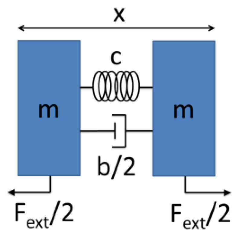
2.2. Nonlinear Model of the Langevin Transducer

For simplifying the model, schematically represented in Figure 3, the transducer is reduced to a one-dimension mass-spring-damper system, excited by external forces F_ext [17]. Using a pair of symmetric external forces, the barycenter remains unchanged.

Figure 3. Simplified electromechanical model of a Langevin transducer.

Figure 3. Simplified electromechanical model of a Langevin transducer.

The external forces are originated in the piezoelectric ceramics and are proportional to the input voltage. The force F_ext can be expressed as the mechanical stress T multiplied by the transducer area A:

$$F_{ext}=-TA$$

(7)

Newton equations of the coupled system can be reduced to an equivalent spring-mass-damper system, where x is the deformation of the structure, showed in Figure 3. Therefore, the equivalent application of Newton’s law can be written as:

$$m\ddot{x}=-b\dot{x}-TA$$

(8)

The stress term in Equation (8) can be replaced by the using the linear expression given by Equation (1a):

$$m\ddot{x}=-b\dot{x}-A\left(cS-eE\right)$$

(9)

where m is the mass of the metallic end elements of the transducer, c is the elastic constant in the longitudinal direction, and b involves the energy losses. Here, the elastic constant c and the piezoelectric coefficient e correspond to c₃₃ and e₃₃, respectively.

A steady state condition is assumed and both amplitudes, X₀ and X₋₁, are considered as known constants, depending only on the angular frequency ω. Replacing Equation (6) in Equation (9) derives:

$$m\ddot{x}=-b\dot{x}-A\left[\left(c_0+\alpha \langle X\rangle \right)S-eE\right]$$

(10)

Considering the proportionality between the electric field and the external voltage, in addition to the proportionality between the strain and the mechanical deformation x(t) the following equation is obtained:

$$\ddot{x}+B\dot{x}+{\omega }_0^{2}x+K.\langle X\left(\omega \right)\rangle x=C{v}_{ext}$$

(11)

The coefficients of Equation (11) are defined as follows:

$$B=\frac{b}{m}$$

(12.1)

$${\omega }_0^2=\frac{c_{0}A}{ml}$$

(12.2)

$$K\left(\omega \right)=\frac{\alpha A}{ml}$$

(12.3)

$$C=\frac{Ae}{ml}$$

(12.4)

For simplifying the model, the end-masses are considered as punctual bodies and l is the thickness of the piezoceramic stack. Assuming that ˂X(ω)˃ is a constant for the sinusoidal steady state, Equation (11) can be solved as an ordinary differential equation. However, this hypothesis is valid only for the analysis in the sinusoidal steady state. A third hypothesis is that the displacement x(t) is sinusoidal, with the same angular frequency ω as the input voltage, as in Equation (4). This frequency domain model does not take into account the generation of harmonics due to the nonlinear behavior. By grouping the terms, the Equation (11) can be rewritten as:

$$\ddot{x}+B\dot{x}+{\omega }_x^{2}x=C{v}_{ext}$$

(13)

The relation between the nonlinear resonance frequency ω_x and the natural frequency ω₀ is given by the following equation:

$${\omega }_x^2={\omega }_0^2+K.\langle X\left(\omega \right)\rangle$$

(14)

The term $K\langle X\left(\omega \right)\rangle$ contains both nonlinear parameters α and β, introduced in the previous section. Solving Equation (13) for a monochromatic input of angular frequency ω, we obtain:

$$X\left(\omega \right)=\frac{C}{\sqrt{{\left({\omega }_x^2-{\omega }^2\right)}^2+B^2{\omega }^2}}·V$$

(15)

This dependence can be verified experimentally and the parameters [C, B, ${\omega }_0^2$, K, β] can be adjusted with a minimization algorithm. As ω_x² depends on X, Equation (15) must be solved iteratively. Assuming that all parameters are known, the process for obtaining the amplitude X can be summarized in three steps: First, introduce the value for the previous step, X₋₁, and the initial value for the actual amplitude, X, for each angular frequency ω. Second, calculate the ω_x² value by using Equation (14), and finally calculate the new value of the amplitude X.

Figure 4. Iterative scheme for solving the model.

Figure 4. Iterative scheme for solving the model.

If the difference between two consecutive values of X is higher than a desired threshold (0.1% in this example), the previous step calculation is repeated (Figure 4). At the end the process, a steady state solution is converged. This algorithm solves the model only for single-valued frequency responses and fails in the case of frequency responses presenting multiple solutions for each frequency. This problem occurs only at regimes presenting extremely high amplitudes, imposing a limitation on the model application.

The output of the model is the amplitude X(ω), as in Equation (15). However, sometimes experimental data is given as velocity. This can be easily obtained by multiplying the amplitude X(ω) by the angular frequency ω.

In order to adjust the parameters, the Nelder-Mead algorithm was employed [19]. It is implemented using the fminsearch function in Matlab and its purpose is to find the optimal values of the set [C, B, ω₀², K, β]. The objective function of the minimization is the sum over the frequency spectra of the quadratic error. The error is computed as the mean square root of the difference between the experimental data and the outputs from the models for each parameter set.

Figure 5 illustrates an example for the calculated response results obtained considering the parameters: B = 600 s⁻¹, C = 4 ms⁻²V⁻¹, ω₀ = 167 krad/s, K = −1.5 × 10⁹ m⁻¹s⁻², and β = 1. This set of values is the initial condition for the minimization described in the next section. The negative sign for the coefficient K is expected, as the frequency decreases with the amplitude X.

Figure 5. Velocity response curve obtained by the model. Here, the input voltage was increased from 1 V to 5 V, with steps of 1 V. Black curves were obtained by increasing the frequency, whereas gray curves are associated with those responses obtained during frequency decreases.

Figure 5. Velocity response curve obtained by the model. Here, the input voltage was increased from 1 V to 5 V, with steps of 1 V. Black curves were obtained by increasing the frequency, whereas gray curves are associated with those responses obtained during frequency decreases.

The model can predict a linear relationship between the square of the frequency and the amplitude neighboring the linear solution ω₀. In order to obtain this approximation, Equation (15) must be differentiated in respect to ω, which is equivalent to:

$${\omega }_{max}^2={\omega }_0^2-B^2+K{X}_{max}$$

(16)

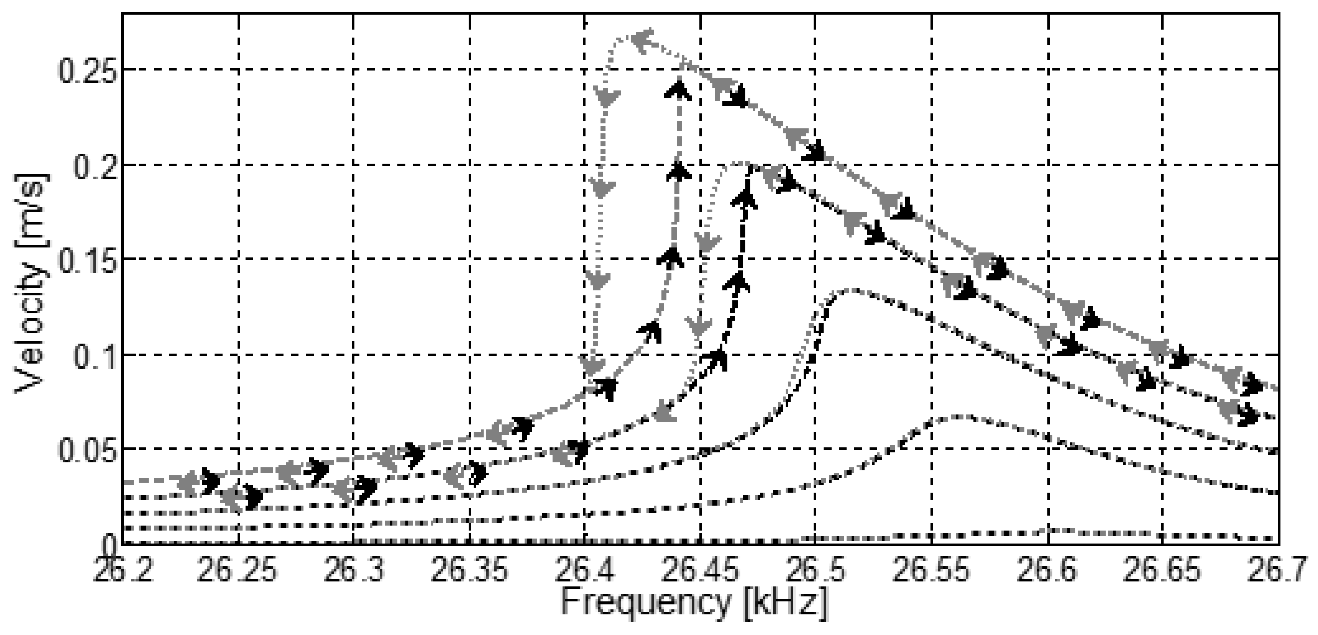
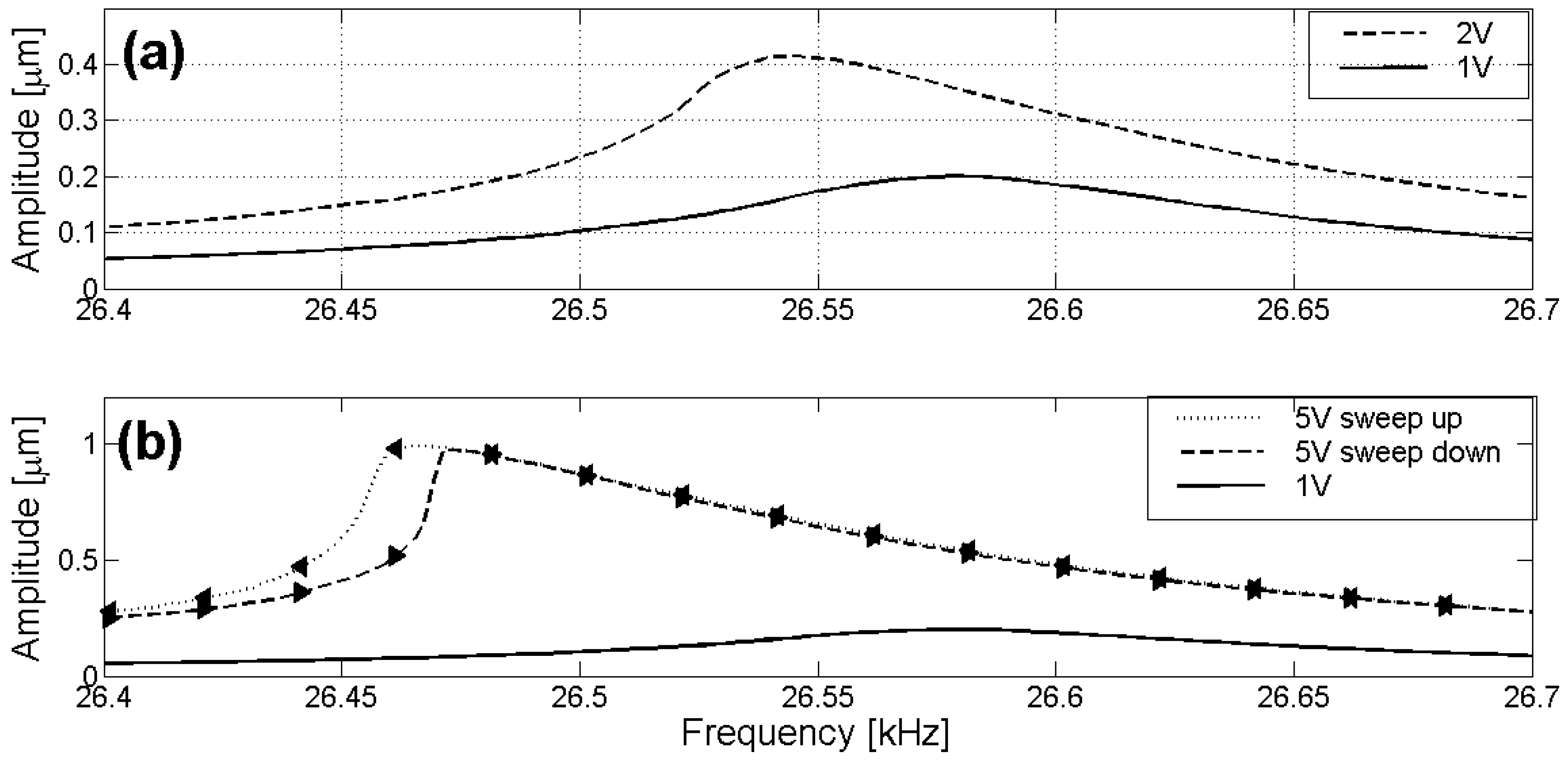
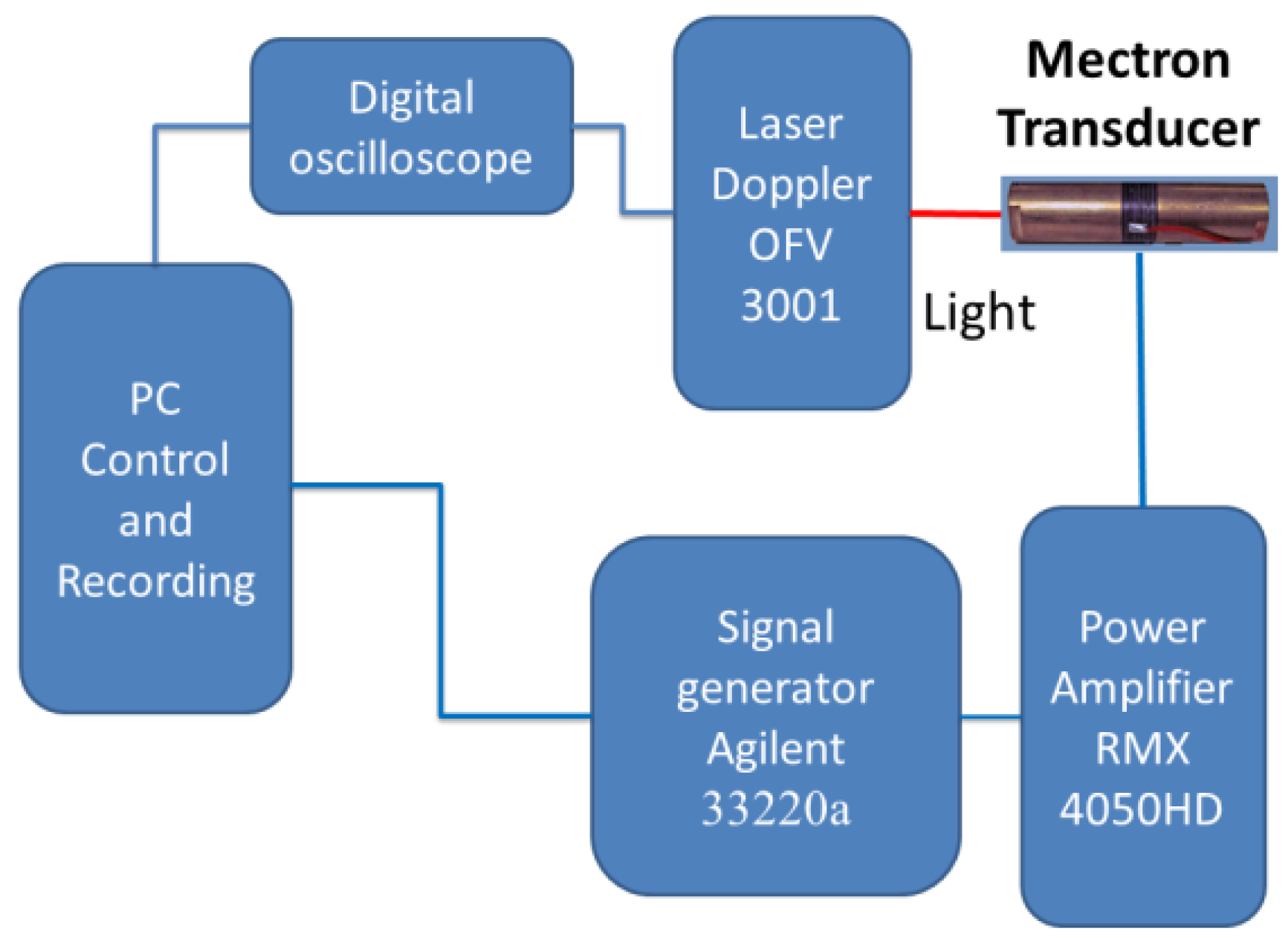
3. Experimental Results

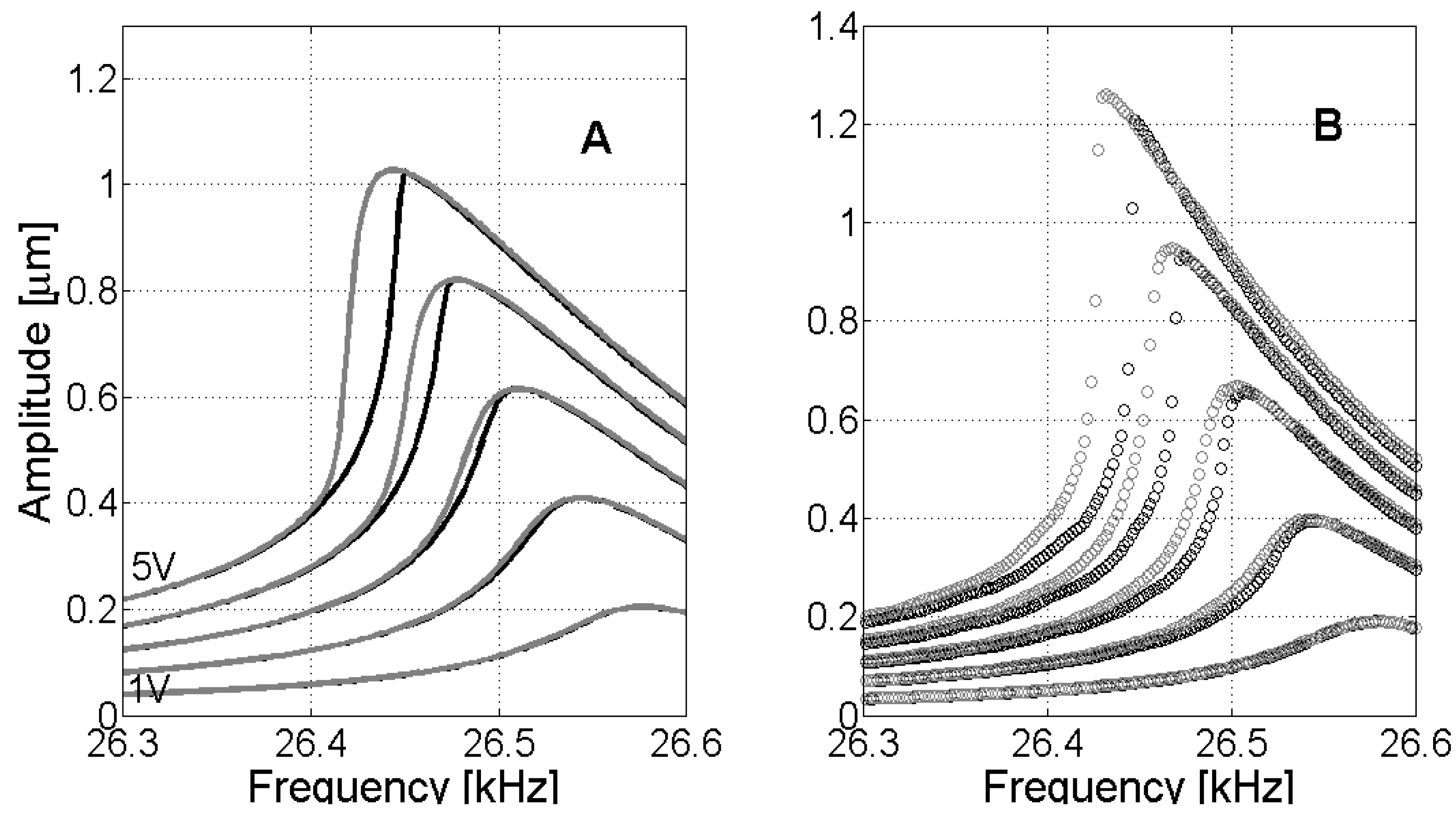
In order to verify the proposed model, the vibration velocity response of a 26 kHz transducer (Mectron Medical Technology, Via Loreto, Italy) is measured, using an optical interferometer, for frequencies neighboring the main resonance frequency. The experiment is repeated for the five voltage levels between 1 V and 5 V, sweeping the driving frequency up and down in each case. A LabView program was developed for externally driving a signal generator (Agilent 33220a, Santa Clara, CA, USA), connected to a power amplifier (QSC Audio, RMX 4050HD, Costa Mesa, CA, USA), used for exciting the ultrasonic transducer. A single point Laser Doppler Vibrometer (Polytec, OFV 3001, Waldbronn, Germany) was used for measuring the vibration velocity at the face of the transducer. Figure 6 shows the schematic setup diagram.

Figure 6. Experimental setup.

Figure 6. Experimental setup.

The displacement amplitude of the vibration is obtained by assuming a sinusoidal response and dividing it by the angular frequency. Adopting the experimental results, the model was adjusted in order to minimize the difference between its output and the experimental data. Figure 7 shows the response curves for the five selected voltages, obtained from sweeping the excitation frequency up and down. Through a numerical implementation in Matlab, as shown in Figure 4, and by applying the Nelder-Mead algorithm for minimizing error, the following coefficients are obtained for a 26 kHz transducer: B = 748 s⁻¹, C = 25.55 m·s⁻²V⁻¹, ω₀ = 167.2 krad·s⁻¹, K = −8 × 10⁸ m⁻¹s⁻². For this case, the non-dimensional parameter is β = 5.

Figure 7. (A) Adjusted model (continuous line), and (B) experimental data (dots). Black curves are obtained by sweeping the driving frequency up; gray curves are obtained when the driving frequency is swept down.

Figure 7. (A) Adjusted model (continuous line), and (B) experimental data (dots). Black curves are obtained by sweeping the driving frequency up; gray curves are obtained when the driving frequency is swept down.

As it can be seen in Figure 7, the frequency shifts and the frequency hysteresis phenomena are both qualitatively represented. For evaluating the quantitative aspect of the model, the main characteristics from both results are summarized in Table 1.

Table 1. Experimental and Numerical results.

	Experimental			Numerical
Voltage [V]	Maximum Displacement Amplitude [μm]	Frequency of Maximum Displacement [kHz]	Hysteresis [Hz]	Frequency of Maximum Displacement [kHz]	Maximum Displacement Amplitude [μm]	Hysteresis [Hz]
1	0.19	26.580	0.25	26.577	0.20	1
2	0.40	26.544	7	26.543	0.41	3
3	0.67	26.502	12	26.510	0.61	7
4	0.95	26.467	15	26.477	0.82	14
5	1.26	26.431	20	26.444	1.03	20

Table 1. Experimental and Numerical results.

	Experimental			Numerical
Voltage [V]	Maximum Displacement Amplitude [μm]	Frequency of Maximum Displacement [kHz]	Hysteresis [Hz]	Frequency of Maximum Displacement [kHz]	Maximum Displacement Amplitude [μm]	Hysteresis [Hz]
1	0.19	26.580	0.25	26.577	0.20	1
2	0.40	26.544	7	26.543	0.41	3
3	0.67	26.502	12	26.510	0.61	7
4	0.95	26.467	15	26.477	0.82	14
5	1.26	26.431	20	26.444	1.03	20

In Table 1, the maximum displacement amplitudes are obtained when the frequency is swept down (gray curves in Figure 7). These values exhibit a significant mismatch comparing with the results obtained during frequency sweep up (black curves). In Table 1, the frequencies at maximum displacement are those excited during the sweep down case. The hysteresis values shown in Table 1 correspond to the maximum difference between the gray and black curves. To evaluate the linear relationship presented in the previous section, the square of the angular frequency is plotted versus the displacement X in Figure 8.

Figure 8. Evaluation of the theoretical model applying Equation (16). Dots are experimental and simulated data taken from Table 1. The continuous gray line is the interpolation of the numerical model, whereas the black dashed line is the linear approximation of the fist three elements in the experimental data.

Figure 8. Evaluation of the theoretical model applying Equation (16). Dots are experimental and simulated data taken from Table 1. The continuous gray line is the interpolation of the numerical model, whereas the black dashed line is the linear approximation of the fist three elements in the experimental data.

As it can be observed in Figure 8, the model and the experimental data are in good agreement ranging from 0 to 0.7 μm. For the case of higher amplitudes, the model predicts a change in the frequency greater than the real one. Note that the major divergence between the numerical and the experimental data is during the transducer operation at high displacements. In this case, thermal effects can be important, changing the speed of the propagation in the materials and the value of the resonant frequency.

4. Conclusions

A simple model for describing the nonlinear vibration behavior of a Langevin transducer was presented. The model was inspired on the Rayleigh law for ferromagnetic materials and requires only two parameters in order to simulate the nonlinear behavior of the transducer. For verifying the proposed model, the frequency response of a 26 kHz Langevin transducer was measured experimentally by performing frequency sweeps, up and down, for different values of amplitude voltage. The comparison between the model and the experimental results confirms the capability of the model for predicting the resonance frequency shifts, breaking of symmetry of the transducer response curve and the frequency hysteresis phenomena for moderate amplitude levels. The proposed model can be implemented in frequency control systems of Langevin transducers ensuring that the transducer will operate with maximum displacement amplitude.

References

1. Iula, A.; Lamberti, N.; Pappalardo, M. An approximated 3-D model of cylinder-shaped piezoceramic elements for transducer design. IEEE Trans. Ultrason. Ferroelectr. Freq. Control. 1998, 45, 1056–1064. [Google Scholar] [CrossRef] [PubMed]
2. Lasky, M. Review of undersea acoustics to 1950. J. Acoust. Soc. Am. 1977, 61, 283–297. [Google Scholar] [CrossRef]
3. Gallego-Juárez, J.A.; Rodriguez, G.; Acosta, V.; Riera, E. Power ultrasonic transducers with extensive radiators for industrial processing. Ultrason. Sonochem. 2010, 6, 953–964. [Google Scholar] [CrossRef] [PubMed]
4. Iula, A.; Parenti, L.; Fabrizi, F.; Pappalardo, M. A high displacement ultrasonic actuator based on a flexural mechanical amplifier. Sens. Actuators A Phys. 2006, 135, 118–123. [Google Scholar] [CrossRef]
5. Alvareda, A.; Pérez, R.; Casals, J.A.; García, J.E.; Ochoa, D. Optimization of elastic nonlinear behavior measurements of ceramic piezoelectric resonators with burst excitation. IEEE Trans. Ultrason. Ferroelectr. Freq. Control. 2007, 54, 2175–2188. [Google Scholar] [CrossRef]
6. Umeda, M.; Nakamura, K.; Takahashi, S.; Ueha, S. An Analysis of Jumping and Dropping Phenomena of Piezoelectric Transducers using the Electrical Equivalent Circuit Constants at High Vibration Amplitude Levels. Jpn. J. Appl. Phys. 2000, 39, 5623–5628. [Google Scholar] [CrossRef]
7. Guyomar, D.; Aurelle, N.; Eyraud, L. Piezoelectric Ceramics Nonlinear Behavior. Application to Langevin Transducer. J. Phys. III 1997, 7, 1197–1208. [Google Scholar] [CrossRef]
8. Guyomar, D.; Aurelle, N.; Richard, C.; Gonnard, P.; Eyraud, L. Nonlinear behaviour of an ultrasonic transducer. Ultrasonics 1996, 34, 187–191. [Google Scholar]
9. Hall, D.A. Nonlinearity in piezoelectric ceramics. J. Mater. Sci. 2001, 36, 4575–4601. [Google Scholar] [CrossRef]
10. Blackburn, J.; Cain, M. Nonlinear piezoelectric resonance: A theoretically rigorous approach to constant I−V measurements. J. Appl. Phys. 2006, 100. [Google Scholar] [CrossRef]
11. Blackburn, J.; Cain, M. Non-linear piezoelectric resonance analysis using burst mode: A rigorous solution. J. Phys. D Appl. Phys. 2006, 40, 227–233. [Google Scholar] [CrossRef]
12. Guyomar, D.; Ducharne, B.; Sebald, G. High nonlinearities in Langevin transducer: A comprehensive model. Ultrasonics 2011, 51, 1006–1013. [Google Scholar] [CrossRef] [PubMed]
13. Pérez, N.; Franceschetti, N.; Adamowski, J.C. Effects of Nonlinearities in Power Ultrasonic Transducers Using Time Reversal Focalization. Phys. Proc. 2010, 3, 161–167. [Google Scholar] [CrossRef]
14. Pérez, N.; Franceschetti, N.; Buiochi, F.; Adamowski, J.C. Short pulse characterization of nonlinearities in power ultrasound transducers. ABCM Symp. Ser. Mechatron. 2010, 4, 793–801. [Google Scholar]
15. Pérez, N.; Andrade, M.A.B.; Buiochi, F.; Adamowski, J.C. Nonlinear Iterative Model for Langevin Ultrasonic Transducers. In Proceedings of the Internoise, Lisboa, Portugal, 13–15 June 2010.
16. Merkeer, T. Standards on Piezoelectricity 176–1987. IEEE Trans. Ultrason. Ferroelectr. Freq. Control 1996, 43, 717–772. [Google Scholar]
17. Rayleigh, L. On the behavior of iron and steel under the operation of feeble magnetic forces. Phil. Mag. 1887, 23, 225–245. [Google Scholar] [CrossRef]
18. Damjanovic, D.; Demartin, M. The Rayleigh law in piezoelectric ceramics. J. Phys. D Appl. Phys. 1996, 29, 2057–2060. [Google Scholar] [CrossRef]
19. Nelder, J.A.; Mead, R. A simplex-method for function minimization. Comput. J. 1965, 7, 308–313. [Google Scholar] [CrossRef]