Evaluating the Impact of an Active Labour Market Policy on Employment: Short- and Long-Term Perspectives

Abstract

The Labour Market Insertion Contract was an Active Labour Market Policy introduced in Spain. It was aimed at individuals who had difficulties entering the labour market, and it was introduced with the purpose of reducing the rate of unemployment. This article provides an estimation of the average impact that this contract had on the employability of individuals in the short and long term. A microeconomic analysis was carried out based on causal statistical inference by using propensity score matching and kernel and radial estimators. Data was taken from the most comprehensive database available, which is the Continuous Sample of Work Histories. Results are consistent with literature reports and show that the employability of participants was inferior to that of individuals with similar, temporary-type contracts. This research contributes to the literature by evaluating whether there was empirical evidence to support the political decision to revoke or replace this kind of direct employment programme.

1. Introduction

In 2006, Spanish authorities decided to revoke the “insertion contract” which was in force in Spain between 2002 and 2006, and which was a type of direct employment programme implemented primarily within the Spanish public sector (Kluve 2010). This decision was supported by Spanish Law 43/2006 (BOE 2006). This Active Labour Market Policy (ALMP) was revoked because it had not met the expectations for which it was put into force. The insertion contract was oriented towards groups of individuals who had difficulties entering the labour market, and it was introduced with the purpose of reducing the rate of unemployment.

The revocation of this contract coincided with the announcement by Spanish authorities of a new contract with similar features which would substitute for it. This new contract, or ALMP, termed “contract with insertion companies for the unemployed at risk of social exclusion” was put into force one year after the enactment of Spanish Law 44/2007 (BOE 2007). Both the revoked, and the new contract were designed as ALMPs for individuals with problems accessing the labour market. Both contracts were oriented to the same integration objectives. The latter contract is still in force.

This research evaluates whether there was empirical evidence for the decision by the Spanish authorities to revoke the insertion contract. To achieve this, it was tested whether the insertion contracts impacted positively or negatively on their recipients. As the new contact is still in force, its evaluation is relevant from a policymaking perspective.

The objective of this paper is to evaluate the decision of the Spanish authorities to revoke the insertion contract. To achieve this, the impact of the insertion contract on the employability of individuals under 30 years of age that signed up to the programme is evaluated. This group was selected due to the high rates of unemployment among young people in Spain. In 2001, Spanish rates of unemployment among the young were 29.11% for the 16–19 years age bracket; 18.86% for 20–24 years; and 13.12% for 25–29 years. For 2006, the rates of unemployment were 28.99%, 14.82% and 10.25%, respectively, all of which were above the overall national rate of unemployment (INE 2012).

To achieve the objective of the paper, a microeconomic analysis was carried out based on causal statistical inference. In compliance with this methodology, a group of participants (formed by individuals who were recipients of an insertion contract) was selected, together with a control group (formed by individuals who signed a temporary employment contract). The database used was the Continuous Work History Sample (Muestra Continua de Vidas Laborales-MCVL) from the Department of Employment and Social Security (Ministerio de Empleo y Seguridad Social 2010) and the period of analysis encompassed the years 2002–2006.

Estimations for both the short- and medium-term impact of the insertion contract were made, measuring its effect on participant employment outcomes at one and three years after completion of the programme.

This paper contributes to the literature by providing, for the first time, an economic evaluation of the impact of the insertion contract for an EU country. The results show a negative impact of this type of contract on the employability of participants in both the short and medium term, which is in keeping with the results of other studies reported in the literature for this type of economic evaluation.

Regarding the structure of this paper, after the Introduction, Section 2 describes the main characteristics of the insertion contract. Section 3 describes he methodology used, and Section 4 outlines the database and defines the variables constructed. Section 5 shows the results obtained and the discussion. The conclusions are summarised in Section 6 and finally, brings together the lessons learned.

2. The Labour Market Insertion Contract

Spanish Law 12/2001 introduced several reforms to Spanish ALMPs with a view to reducing serious pockets of unemployment in specific groups (BOE 2001). The reforms were designed to increase professional experience and to improve the labour skills of recipients (Cansino and Sánchez-Braza 2010, 2011). In 2001, the rate of unemployment in the EU was 8.5% compared to 10.3% in Spain, placing the latter in the top ten countries in the EU ranked according to high rates of unemployment (Eurostat 2012).

One of the reforms introduced was the new insertion contract, which formed the basis for a type of direct employment programme. Recipients of the contract had to be registered as unemployed with the Public Employment Service in order to benefit from this form of insertion into the labour market. Spanish legislation had previously contemplated (Law 64/1997) the implementation of ALMPs for groups of individuals with problems accessing the labour market (BOE 1997).

Improvement in the employability of a person achieves the simultaneous improvement both of the individual and collective conditions (Quintanilla 2001). As such, the insertion contract was implemented with a view to increasing the likelihood of employment for recipients who completed the programme.

This type of contract was mainly offered by the Public Administration, but non-profit organizations also participated in the programme as employers. The jobs offered were related to works and services of collective utility, for their contribution to cultural development, conservation of the environment, and social assistance services, among others. The duration of the contract was for a maximum period of nine months, following which it was not possible to sign another contract of the same type within the subsequent three years. This period is similar to that of most AMPLs, which usually last for four to six months (Card et al. 2010). Once completed, the contract did not provide any compensatory remuneration for the worker.

In this research, the period considered includes the entire period during which the insertion contract was in force, from 1 January 2002 to 31 December 2006 when the programme was revoked. For the first year, total funding for the ALMP accounted for 0.7% of the Spanish GDP and, for 2006, this figure was equal to 0.8% of the GDP (OECD 2014).

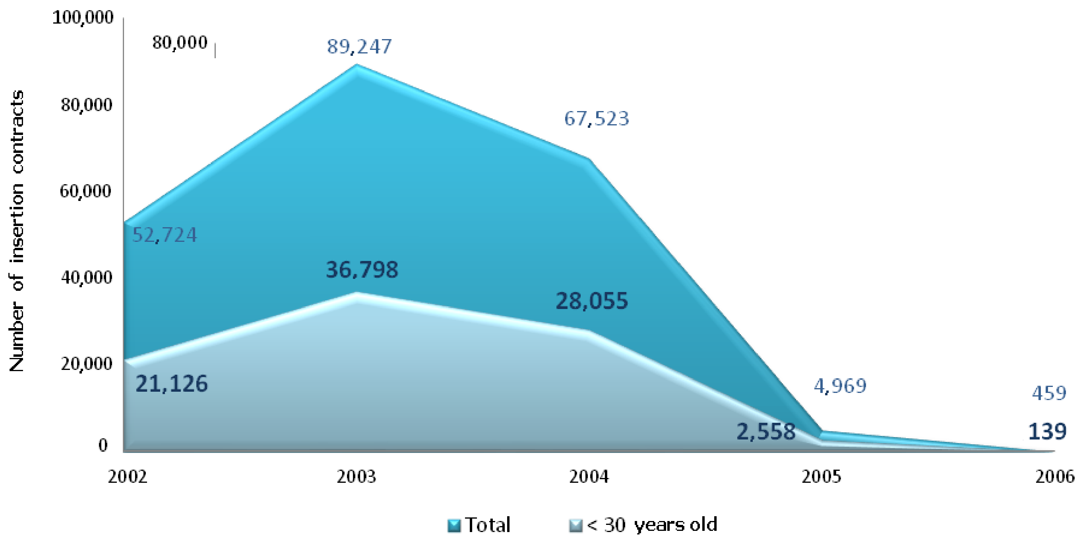
In 2006, 214,922 insertion contracts were signed, of which 88,676 contracts were signed by individuals under 30 years of age. According to the data obtained from the MCVL, in some cases the same individual signed an insertion contract more than once. Therefore, the number of individuals who were awarded this contract is lower than the number of insertion contracts actually signed. Figure 1 shows the evolution of insertion contracts signed from 2002 until the programme was discontinued, as well as the number of insertion contracts signed by individuals under 30 years of age.

3. Methodology

3.1. The Potential Outcomes Model

Within the realm of public policy evaluation, statistical causal inference allows determination of the impact (the cause) of a certain policy on one or more variables of interest (the effect). This methodology facilitates the attainment of consistent estimators of the effect of the programme by controlling for the possible influence of other factors on the variables of interest. Thus, the purpose of this methodology is to isolate the effect of this policy on the variable of interest by maintaining control over other contaminating factors that may affect these variables. Techniques of causal inference have been used in multiple scientific fields, such as medicine (Hirano and Imbens 2001; Rosenbaum 2002) or the political sciences (Duch and Stevenson 2006; Imai 2005), among others.

The development of evaluation methods based on statistical causal inference can be found in the Potential Outcomes Model (POM), which allows comparison of the variables of interest between participants and non-participants in public programmes (Imbens and Wooldridge 2009). Prominent models have been developed based on the Rubin Causal Model (RCM) (Rubin 1974, 1978). According to Rubin (1974), and subsequent contributions by Holland (1986), to determine the causal effect of a specific policy on each participant it is necessary to define a treatment indicator. Thus, a binary variable D_i ϵ {0, 1} is defined which indicates whether an individual has participated (D_i = 1), or not (D_i = 0).

After specifying the indicator, it is necessary to determine the response variable, defined as the variable of interest, the effect by which the effectiveness of the evaluated policy is to be measured. This response variable is defined in terms of potential responses which are associated with the values of the treatment indicator (having, or not having, participated in the programme).

As such, Y_1i will be the potential response of individual i when D_i = 1, meaning that individual i has participated in the evaluated policy. On the other hand, Y_0i will be the potential response of individual i when D_i = 0, meaning that individual i has not participated in the evaluated policy.

$$Y_i\{\begin{array}{c}{Y}_{1i}if{D}_i=1\\ Y_{0i}if{D}_i=0\end{array}$$

(1)

From the above, the programme’s causal effect on the response variable is determined by the difference [Y_1i – Y_0i], thus allowing an evaluation of the effectiveness of the programme.

It is easy to prove how a counterfactual event is linked to the response variable. Obviously, it is not possible to observe both responses, Y_1i and Y_0i, simultaneously, but rather just one of the two possible values of Y_i. If the individual participates in the policy (D_i = 1) the value Y_1i will be observed, otherwise the value of Y_0i will be obtained for a non-participant (D_i = 0). Ultimately, for each individual the only response which can be obtained is Y_i, which is defined as:

$$Y_i=D_i{Y}_{1i}+(1-D_i)Y_{0i}$$

(2)

According to Holland (1986), the known fundamental problem of identification in causal studies arises which makes it impossible to determine the individual causal effects of the programme. This fact, based on the counterfactual nature of the potential responses, requires searching for a second-best alternative, which is derived by estimating average causal effects.

To determine the causal effect, an average effect is calculated, which usually involves one of the several specifications. The average treatment effect, ATE, is defined as the difference between the average values of the response variable of the individuals that participated in the programme, and those that did not.

$${\widehat{\alpha }}_{ATE}=E(Y_1-Y_0)=E(Y|D=1)-E(Y|D=0)$$

(3)

The average treatment effect on the treated, ATET, is calculated as the difference between the average of the response variable of participating and non-participating individuals, but only for the participating individuals; it is given by:

$${\widehat{\alpha }}_{ATET}=E(Y_1-Y_0|D=1)=E(Y_1|D=1)-E(Y_0|D=1)$$

(4)

Basically, these average effects are obtained by comparing treated individuals of the programme (treatment group) with untreated individuals (control group).

In the case of random experiments, individuals are randomly assigned to treatment and control groups. This ensures independence between potential responses and possible participation in the programme. This independent status is known as the unconfoundedness condition, and is represented as:

$$(Y_1,Y_0)\perp D$$

(5)

However, in observational studies this random assignment is not usually done. Then, the estimation of causal effect must be inferred from the available observational data in a non-experimental context. Regardless of this, it is necessary to ensure fulfilment of the unconfoundedness condition in order to obtain an accurate estimation of the average effect. To overcome this restriction, observational methods reproduce the experimental scenario, thus ensuring independence between potential responses and the participating indicator of the programme. The use of statistical causal inference methods, such as the proposed propensity score matching, allows individuals in the treatment group and the control group to be homogenized, enabling the comparison between both groups, while eliminating the possible dependence between D and Y.

3.2. Methods of Selection on Observables

The quality of the estimation of average effects could be diminished if individuals in both the participant and control groups differ in characteristics other than those arising from participation in the evaluated programme. However, to the extent that these features can be observed, and individuals (participants and controls) differ only in terms of these characteristics, such differences can be controlled for. This is the foundation on which the methods of selection on observables is based.

The covariate X_j is defined as a default variable with respect to D if, for each and every one of the observed individuals, the values of X_j do not depend on D_i (Rubin 1978). More generally, the vector of covariates (X = X₁, X₂, …, X_n) can be defined as a set of independent covariates of D_i for each and every one of the considered observations. Isolating the contaminant effects of these observable characteristics (called covariates) facilitates comparison between participants and control individuals.

Following Heckman and Hotz (1989), and Heckman et al. (1998), the selection of observables proceeds when the dependence between D and Y is due to the influences of covariate X in the process of allocating individuals, so that, by controlling X the selection bias is solved, thus eliminating the possible dependence between D and Y.

In the selection of observables, once the independence condition has been assured, it is possible, following Dehejia and Wahba (1999), to express the average effect of the policy evaluated as:

$$(Y_1,Y_0)\perp D|X$$

(6)

Thus, the selection bias problem is settled by conditioning the values of the response variable to the values of the vector of covariates, X.

3.3. Propensity Score Matching

Among the methods of selection of observables, and according to the characteristics of the evaluated policy, the propensity score matching method was selected for this research.

The matching technique consists of obtaining pairs of similar individual observable characteristics, with the only difference being that one individual belongs to the participant group and the other to the control group. If the pairing of these individuals includes all of these covariates, the matching provides an unbiased estimate of the effects of a policy by comparing these pairs of individuals.

However, the existence of a large number of covariates might turn the pairing process between individual participants and control non-participants into a very complicated process.

For this reason, the propensity score is invoked. Rosenbaum and Rubin (1983) define the propensity score as the probability that any given individual in the sample can participate in the programme (probability that D_i = 1), conditioned by the values taken by X.

$$\epsilon (X)=P(D=1|X)$$

(7)

The calculation of the propensity score ε(X) facilitates the operation by reducing a large number of covariates to a single variable (Abadie and Imbens 2016; Hahn 1998). The proposition of independence is thus formulated as:

$$(Y_1,Y_0)\perp D|\epsilon (X)$$

(8)

Since the propensity score ε(X) is a function of X, this probability depends on the assumption about its distribution function, which must be estimated from the sample data. This can be expressed as follows:

$$\epsilon (X)=P(D=1|X)=F(\beta X)$$

(9)

where β is the vector of parameters associated with the vector of covariates X.

To estimate the propensity score, different models of binary response (choice) can be specified; the two most commonly used being the probit and logit models.

The probit model considers that F is the standard normal cumulative distribution function. In this model, the probability is determined as follows:

$$P{(D_i=1|X)}_{probit}={\displaystyle {\int }_{-\infty }^{\alpha +X_i^{\prime }\beta }{\left(\frac{1}{\sqrt{2\pi }}\right)}^{\frac{-z^2}{2}}dz}\mathrm{for}-\infty <z<\infty$$

(10)

In the logit model, F is specified as the cumulative distribution function of the logistic distribution:

$$P{(D_i=1|X)}_{logit}=\frac{e^{(\alpha +X_i^{\prime }\beta )}}{1+e^{(\alpha +X_i^{\prime }\beta )}}$$

(11)

The regression parameters β can be obtained by using MLE, maximizing the log-likelihood function:

$$\left(\beta \right)={\displaystyle \sum _{i=1}^N{D}_i\ln \left[F(\alpha +X_i^{\prime }\beta )\right]+(1-D_i)\ln \left[1-F(\alpha +X_i^{\prime }\beta )\right]}$$

(12)

There are no defined selection criteria for choosing either one or other model to estimate the propensity score. Hence, the selection is made merely for operational reasons. After estimating both models, the one which maximizes the value of the likelihood function is chosen.

At a second stage, from the estimated values of the propensity score for each individual and taking into account that individuals with equal or similar propensity scores are similar individuals, the process of pairing or matching follows. Each individual in the treatment group with a given value of ε_1i is appointed one individual (or various) from the control group with ε_0j, such that they present a similar distribution of X. Thus, by isolating the possible contaminating effect of covariates, the matching provides an unbiased estimate of the effect of carrying out the programme.

The possibility of finding individuals in the participant and control groups with identical propensity score values can, however, be greatly lowered. Therefore, the kernel and radial matching methods (Becker and Ichino 2002; Heckman et al. 1997) were used, which provide a solution based on matching (using different techniques) those individuals with similar propensity score values.

The radial method establishes a radius (r) which assigns individuals of the control group whose ε_0j is within the range formed by r and ε_1i, to each individual participant with a given propensity score, ε_1i.

The matching condition for the radial method is expressed as:

$$C(i)=\left\{{\epsilon }_0|\Vert {\epsilon }_1-{\epsilon }_0\Vert <r\right\}$$

(13)

where C(i) is the control individual fulfilling the matching condition, and ε₁ and ε₀ correspond to the individual and control participants’ propensity scores, respectively.

Of the two types of average effect defined above, ATE and ATET, ATET is chosen for this evaluation as it is the most commonly used in the evaluation techniques based on propensity score matching (Abadie and Imbens 2006; Dehejia and Wahba 2002; Heckman et al. 1998).

Thus, the ATET estimator of the radial method is expressed as:

$${\widehat{\alpha }}_{ATET(radial)}=\frac{1}{n_1}{\displaystyle \sum _{i=1}^{n_1}}(Y_{1i}-{\displaystyle \sum _{j=1}^{C(i)}}{w}_{ij}{Y}_{0j})$$

(14)

In this equation, w_j are the weights, defined by w_j = ∑_i w_ij, and where w_ij = 1/N_i ^C and N_i ^C is the number of control individuals matched with the participating individual i.

The kernel method, on the other hand, matches all participant individuals with the weighted average propensity score of the control individuals. The weighting is inversely proportional to the difference in propensity score between participants and control individuals. Thus, the kernel method weights the proximity between the participant and control individuals. The ATET estimator of the kernel method is expressed as:

$${\widehat{\alpha }}_{ATET(kernel)}=\frac{1}{n_1}{\displaystyle \sum _{i=1}^{n_1}}(Y_{1i}-{\displaystyle \sum _{j\in (D=0)}}{w}_{ij}{Y}_{0j})$$

(15)

For this case, the weighting term is defined as:

$$w_{ij}=K\left(\frac{{\epsilon }_{1i}-{\epsilon }_{0j}}{\theta }\right)/{\displaystyle \sum _{j\in (D=0)}K\left(\frac{{\epsilon }_{1i}-{\epsilon }_{0j}}{\theta }\right)}$$

(16)

where K(•) is a function, which in this case will consist of the application of the Gaussian kernel function. θ is the predefined parameter bandwidth.

4. Database

The database for this research is the MCVL, which was constructed from micro-information extracted from administrative records derived from the social security system, in addition to information from municipal council census records and the tax authorities (García Pérez 2008). The MCVL has grown into a database which is widely used to study characteristics of the Spanish labour market (Clemente 2007; Toharia 2008).

A feature of the MCVL is the availability of administrative information about individuals who are registered within the social security system. A second and important characteristic is that the database registers the dates of joining and leaving regular employment, making it possible to determine an individual’s employment history. The information concerning details of when an individual registers for unemployment subsidies is also available, making it possible to identify periods of unemployment.

Moreover, the MCVL incorporates the previous employment history of each individual within the sample, which dates back to when computerized records commenced. Thus, the database contains relevant information to enable the effects of Spanish ALMPs to be determined in the short, medium and long term.

Also included in the database is information about the demographics, educational level, and the professional group of the individual, as well as economic activity, size of the company and the region. When this is added to the information concerning social security contributions, an extensive and representative sample of the Spanish labour market is obtained.

The MCVL data has been published annually since 2004. The information relating to individuals who continue maintaining their link with the social security system, as contributors or as benefit recipients, is updated every year. Those who died or ceased to be linked to the social security system, disappear from the sample, and are replaced by other individuals, in the same proportion, to maintain the representability of the sample. Also, when a former member re-establishes their link with the social security system, they automatically reappear in the subsequent MCVL figures that are published (García Pérez 2008). So, for the purpose of this research the MCVL editions published from 2004 to 2009 were used.

For the creation of the participant and control groups, a random selection of individuals was obtained in accordance with several characteristics relevant to this research. The treatment group is formed of individuals who signed an insertion contract. For the control group, a random selection was made of individuals who signed a contract with similar characteristics to that of the insertion contract. In this case, the contract closest to the evaluated one that best meets their characteristics was the temporary employment contract. The similarity between the two contracts is that neither requires a specific level of education or a specific age, and both are full-time contracts with a limited duration. The length of the temporary contract is for up to six months, though, on certain occasions, it can be extended to a period of 12 months. Among the contracts which were in force during the period under consideration, this is considered to be the most suitable type to be compared with the insertion contract.

During this period, there were only three other full-time temporary contracts. Each had a specific purpose (substitution, training), or some requirements regarding the level of education or other characteristics. Given that the insertion contract was targeted towards individuals with difficulties entering the labour market, this requirement was considered within the control group by imposing the condition that, to be selected for the control group, the individual had to be registered with the Public Employment Service as being unemployed and not having recorded any long-term employment episodes over recent months.

Also, in order to minimize possible bias, individuals from both groups were required to fulfil the following conditions: First, the minimum period of employment for both contracts was three months. The age of the individuals was to be between 18 and 30 years. According to Spain’s Public Employment Service (SEPE 2012), on average, 40.9% of the individuals who signed the insertion contract fulfilled these characteristics, culminating in the highest proportion reached in 2005 (51.5%) and the lowest in 2006 (30.3%). The second condition to be fulfilled was the non-repetition of the same contract within the period of employment history analysed. For the treatment group, 17.7% of individuals were repeat recipients of the insertion contract. The exclusion of such individuals, and of those in the control group who received second or subsequent temporary contracts, within the period analysed, allowed the effects on employability to be analysed for this specific contract. If this were not the case, when an individual entered into more than one contract, the final effect obtained would be confused between the two contracts. In addition, for each contract, different values could be registered for the covariates considered, which would make it impossible to adequately control these circumstances or characteristics. Thus, with the fulfillment of all these conditions, the fundamental difference between the two groups is the purpose of the labor insertion that includes the contract evaluated. In this sense, the estimated average treatment effect gauges to what extent the insertion contract offers to their recipients, better labor market results in terms of worked days and employability versus those with a similar contract but no insertion purposes.

The period of analysis was from 2002, the year in which the insertion contract entered into force, until 2009, three years after the contract was revoked in 2006.

From the proposed methodology, the variable D is defined as indicative of the signing, or not, of an insertion contract by an individual, i. If D_i takes the value of unity, this implies that the individual i has signed an insertion contract. However, if D_i takes the value of 0, the individual i will be included within the control group as this implies that a temporary contract was signed.

The total size of the selected sample consists of 5294 individuals, of which 1006 constitute the treatment group and 4288 the control group, giving a ratio of approximately 1:3.

To determine the outcome variable, it is defined in terms of the capacity of individuals to find employment, that is, their employability, as stipulated by Zweimüller and Winter-Ebmer (1996). Employability is represented by Y_i (outcome variable) and is constructed as the number of employment days after the termination of the insertion contract.

In order to measure the impact of the contract on both short- and long-term employability, the outcome variable is broken down into two variables which depend on the term under consideration. These variables are defined as Y_i¹ and Y_i² and represent the number of days worked in the year following completion of the contract (short term effect) and the three years following its conclusion (long term effect), respectively.

Finally, in order to guarantee the unconfoundedness condition, a covariates vector which includes five groups of covariates was considered, providing information about the characteristics of the individuals, as well as of the contracts considered. All the covariates that affect the outcome variable of the participants must also exist for the individuals of the control group. The MCVL database provides both groups with the same covariates which will be included in the propensity score matching procedure. Therefore, all possible relevant covariates for which information was available on both groups was included in the analysis, whilst ensuring that the estimated propensity score was balanced.

Table 1. Covariates and descriptive statistics: Total individuals.

Total Individuals
Variable	Description	Obs.	Mean	Std.Dev.
1. Socio-demographic factors. Base category: women with no education.
Gender	1 if male; 0 if female.	2638	0.498	0.500
Age	Age at end of contract, between 18 and 30 years old.	5294	24.563	3.264
Compulsory	1 if has compulsory studies; 0 otherwise.	1977	0.373	0.484
College	1 if has high school studies or similar; 0 otherwise.	1582	0.299	0.458
Degree level	1 if has university studies; 0 otherwise.	985	0.186	0.389
2. Year end and duration of the respective contract. Base category: duration less than 10 months.
Year	1 if contract ends in 2002; 2 if ends in 2003; 3 if ends in 2004; 4 if ends in 2005; 5 if ends in 2006	5294	2.500	1.287
Duration	1 if duration of contract is equal or greater of 10 months (maximum duration: 12 months)	5294	0.231	0.422
3. Profesional group. Base category: workers and similar.
Specialists	1 if Official 3th grade and specialists; 0 otherwise.	806	0.152	0.359
Official	1 if Official 1st and 2nd grade; 0 otherwise.	664	0.125	0.331
Assistant	1 if Assitant and auxiliar without titulation; 0 otherwise.	633	0.120	0.324
Administrative	1 if Administrative auxiliar, administrative and supervisor; 0 otherwise.	1314	0.248	0.432
Engineers	1 if Technical engineers, graduates and senior management; 0 otherwise.	508	0.096	0.295
4. Economic activity. Base category: other unspecified
Agri./Extractive	1 if agriculture and extractive; 0 otherwise.	649	0.123	0.328
Energy/Construction	1 if energy and construction; 0 otherwise.	1509	0.285	0.451
Trade/Hotel/Transport	1 if trade, hotel and transport; 0 otherwise.	438	0.083	0.276
Financial/Property	1 if financial and real estate; 0 otherwise	254	0.048	0.214
Education	1 if educational activities; 0 otherwise.	853	0.161	0.368
Public/Health/Social	1 if public administration, health and other social activities; 0 otherwise.	615	0.116	0.320
5. Community implementation of the respective contract. Base category: Catalonia.
Andalusia	1 if Andalusia; 0 otherwise.	841	0.159	0.366
Aragon	1 if Aragon; 0 otherwise.	117	0.022	0.147
Asturias	1 if Asturias; 0 otherwise.	135	0.026	0.158
Balearic Islands	1 if Balearic Islands; 0 otherwise.	111	0.021	0.143
Basque Country	1 if Basque Country; 0 otherwise.	241	0.046	0.208
Canary Islands	1 if Canary Islands; 0 otherwise.	327	0.062	0.241
Cantabria	1 if Cantabria; 0 otherwise.	88	0.017	0.128
Castile and Leon	1 if Castile and Leon; 0 otherwise.	300	0.057	0.231
Castile-La Mancha	1 if Castile-La Mancha; 0 otherwise.	249	0.047	0.212
Ceuta and Melilla	1 if Ceuta and Melilla; 0 otherwise.	33	0.006	0.079
Extremadura	1 if Extremadura; 0 otherwise.	91	0.017	0.130
Galicia	1 if Galicia; 0 otherwise.	498	0.094	0.292
Madrid	1 if Madrid; 0 otherwise.	761	0.144	0.351
Murcia	1 if Murcia; 0 otherwise.	119	0.022	0.148
Rioja	1 if Rioja; 0 otherwise.	45	0.009	0.092
Valencian Community	1 if Valencian Community; 0 otherwise.	578	0.109	0.312

Source: Own elaboration from MCVL.

shows the description of the covariates and the principal descriptive statistics used for the whole sample for each of these covariates.

Table 2. Covariates and descriptive statistics: Treatment and control groups.

	Participants			Control
Variable	Obs.	Mean	Std.Dev.	Obs.	Mean	Std.Dev.
1. Socio-demographic factors. Base category: women with no education.
Gender	347	0.345	0.476	2291	0.534	0.499
Age	1006	24.904	3.099	4288	24.483	3.297
Compulsory	298	0.296	0.457	1679	0.392	0.488
College	274	0.272	0.445	1308	0.305	0.460
Degree level	287	0.285	0.452	698	0.163	0.369
2. Year end and duration of the respective contract. Base category: duration less than 10 months.
Year	1006	2.405	1.102	4288	2.522	1.326
Duration	1006	0.224	0.417	4288	0.233	0.423
3. Profesional group. Base category: workers and similar.
Specialists	27	0.027	0.162	779	0.182	0.386
Official	43	0.043	0.202	621	0.145	0.352
Assistant	106	0.105	0.307	527	0.123	0.328
Administrative	161	0.160	0.367	1153	0.269	0.443
Engineers	318	0.316	0.465	190	0.044	0.206
4. Economic activity. Base category: other unspecified.
Agri./Extractive	24	0.024	0.153	625	0.146	0.353
Energy/Construction	18	0.018	0.133	1491	0.348	0.476
Trade/Hotel/Transport	13	0.013	0.055	435	0.101	0.302
Financial/Property	24	0.024	0.153	230	0.054	0.225
Education	646	0.642	0.480	207	0.048	0.214
Public/Health/Social	202	0.201	0.401	413	0.096	0.295
5. Community implementation of the respective contract. Base category: Catalonia.
Andalusia	95	0.094	0.293	746	0.174	0.379
Aragon	21	0.021	0.143	96	0.022	0.148
Asturias	30	0.030	0.170	105	0.024	0.155
Balearic Islands	14	0.014	0.117	97	0.023	0.149
Basque Country	35	0.035	0.183	206	0.048	0.214
Canary Islands	98	0.097	0.297	229	0.053	0.225
Cantabria	25	0.025	0.156	63	0.015	0.120
Castile and Leon	70	0.070	0.255	230	0.054	0.225
Castile-La Mancha	92	0.091	0.288	157	0.037	0.188
Ceuta and Melilla	27	0.027	0.162	6	0.001	0.037
Extremadura	7	0.007	0.083	84	0.020	0.139
Galicia	223	0.222	0.416	275	0.064	0.245
Madrid	99	0.098	0.298	662	0.154	0.361
Murcia	10	0.001	0.032	118	0.028	0.164
Rioja	10	0.010	0.099	35	0.008	0.090
Valencian Community	98	0.097	0.297	480	0.112	0.315

Source: Own elaboration from MCVL.

shows the main descriptive statistics for each of the groups with the group distributions for each of the covariates.

5. Results and Discussion

The estimation of the impact of the insertion contract is implemented in two phases. The first phase corresponds to the calculation of the propensity score for each individual. In the second phase, individual participants are matched with control individuals with similar propensity score values (see Cansino et al. 2013).

Table 3. Probit model estimations.

	Variable	(1)		(2)		(3)		(4)		(5)
	Constant	−0.948	***	−0.838	***	−0.166		−0.461	*	−0.671	**
		(0.161)		(0.165)		(0.178)		(0.235)		(0.257)
1. Socio-demographic factors	Gender	−0.411	***	−0.409	***	−0.425	***	−0.360	***	−0.311	***
		(0.042)		(0.042)		(0.048)		(0.062)		(0.065)
	Age	0.015	**	0.015	**	0.000		−0.015		−0.023	**
		(0.006)		(0.006)		(0.007)		(0.009)		(0.010)
	Compulsory	−0.228	***	−0.234	***	−0.165	**	−0.132		−0.100
		(0.064)		(0.064)		(0.065)		(0.091)		(0.093)
	College	−0.195	***	−0.200	***	−0.192	***	−0.188	*	−0.176	*
		(0.067)		(0.067)		(0.072)		(0.097)		(0.101)
	Degree Level	0.157	**	0.156	**	−0.208	**	−0.140		−0.061
		(0.071)		(0.071)		(0.083)		(0.110)		(0.116)
2. Year end and duration	Year			−0.048	***	−0.040	**	−0.020		−0.017
				(0.015)		(0.016)		(0.022)		(0.024)
	Duration			−0.018		−0.039		0.171	**	−0.077
				(0.048)		(0.053)		(0.064)		(0.073)
3. Profesional group	Specialists					−1.165	***	−0.859	***	−0.904	***
						(0.095)		(0.113)		(0.119)
	Official					−0.808	***	−0.498	***	−0.490	***
						(0.086)		(0.114)		(0.116)
	Assistant					−0.359	***	−0.396	***	−0.371	***
						(0.075)		(0.095)		(0.100)
	Administrative					−0.624	***	−0.493	***	−0.423	***
						(0.065)		(0.083)		(0.090)
	Engineers					0.939	***	0.872	***	0.933	***
						(0.082)		(0.105)		(0.113)
4. Economic activity	Agri./Extractive							−0.528	***	−0.480	***
								(0.118)		(0.122)
	Energy/Construction							−0.864	***	−0.941	***
								(0.116)		(0.121)
	Trade/Hotel/Transport							−1.062	***	−1.084	***
								(0.236)		(0.255)
	Financial/Property							−0.124		−0.177
								(0.139)		(0.145)
	Education							1.949	***	1.875	***
								(0.079)		(0.082)
	Public/Health/Social							0.631	***	0.630	***
								(0.084)		(0.087)
5. Community implementation	Andalusia									0.227	*
										(0.127)
	Aragon									0.239
										(0.202)
	Asturias									0.629	***
										(0.169)
	Balearic Islands									0.069
										(0.233)
	Basque Country									0.343	**
										(0.167)
	Canary Islands									0.835	***
										(0.141)
	Cantabria									0.495	**
										(0.210)
	Castile and Leon									0.449	***
										(0.145)
	Castile-La Mancha									0.809	***
										(0.150)
	Ceuta and Melilla									0.794	**
										(0.346)
	Extremadura									−0.349
										(0.328)
	Galicia									1.136	***
										(0.126)
	Madrid									0.106
										(0.127)
	Murcia									−2.006	***
										(0.550)
	Rioja									0.194
										(0.252)
	Valencian Comunity									0.233	*
										(0.123)
	Número Obs.	5294		5294		5294		5294		5294
	Log. Verosimilitud	−2480.9		−2476.4		−2119.7		−1256.8		−1158.7
	Pseudo-R2	0.0363		0.0380		0.1766		0.5118		0.5499
	LR chi2	186.74		195.77		909.20		2634.98		2831.23
	(p-value)	0.000		0.000		0.000		0.000		0.000

Source: Own elaboration MCVL. Note: Standard errors robust to heteroskedasticity in brackets. One, two, or three asterisks indicate coefficient significance at the 10, 5, and 1% levels, respectively.

and

Table 4. Logit model estimations.

	Variable	(1)		(2)		(3)		(4)		(5)
	Constant	−1.599	***	−1.403	***	−0.146		−0.582		−0.920	*
		(0.284)		(0.292)		(0.318)		(0.441)		(0.486)
1. Socio-demographic factors	Gender	−0.731	***	−0.729	***	−0.805	***	−0.641	***	−0.549	***
		(0.075)		(0.075)		(0.088)		(0.119)		(0.123)
	Age	0.027	**	0.027	**	0.001		−0.035	**	−0.051	***
		(0.011)		(0.011)		(0.013)		(0.017)		(0.018)
	Compulsory	−0.408	***	−0.421	***	−0.322	***	−0.243		−0.194
		(0.113)		(0.113)		(0.115)		(0.176)		(0.181)
	College	−0.349	***	−0.361	***	−0.389	***	−0.307	*	−0.291
		(0.118)		(0.118)		(0.128)		(0.185)		(0.193)
	Degree Level	0.255	**	0.252	**	−0.403	***	−0.232		−0.098
		(0.122)		(0.122)		(0.148)		(0.207)		(0.221)
2. Year end and duration	Year			−0.082	***	−0.076	**	−0.029		−0.018
				(0.026)		(0.029)		(0.042)		(0.045)
	Duration			−0.008		−0.088		0.358	***	−0.111
				(0.085)		(0.095)		(0.120)		(0.144)
3. Profesional group	Specialists					−2.311	***	−1.528	***	−1.644	***
						(0.208)		(0.208)		(0.215)
	Official					−1.508	***	−0.915	***	−0.873	***
						(0.172)		(0.208)		(0.217)
	Assistant					−0.661	***	−0.691	***	−0.615	***
						(0.135)		(0.176)		(0.190)
	Administrative					−1.138	***	−0.834	***	−0.719	***
						(0.118)		(0.155)		(0.169)
	Engineers					1.517	***	1.651	***	1.766	***
						(0.138)		(0.197)		(0.217)
4. Economic activity	Agri./Extractive							−1.070	***	−1.009	***
								(0.238)		(0.250)
	Energy/Construction							−2.014	***	−2.133	***
								(0.274)		(0.279)
	Trade/Hotel/Transport							−2.482	***	−2.553	***
								(0.582)		(0.569)
	Financial/Property							−0.346		−0.450
								(0.270)		(0.280)
	Education							3.357	***	3.219	***
								(0.149)		(0.152)
	Public/Health/Social							1.042	***	1.047	***
								(0.156)		(0.164)
5. Community implementation	Andalusia									0.362
										(0.244)
	Aragon									0.451
										(0.369)
	Asturias									1.220	***
										(0.312)
	Balearic Islands									0.219
										(0.432)
	Basque Country									0.677	**
										(0.312)
	Canary Islands									1.591	***
										(0.273)
	Cantabria									0.949	**
										(0.368)
	Castile and Leon									0.776	***
										(0.263)
	Castile-La Mancha									1.443	***
										(0.286)
	Ceuta and Melilla									1.556	**
										(0.606)
	Extremadura									−0.736
										(0.585)
	Galicia									2.110	***
										(0.237)
	Madrid									0.195
										(0.235)
	Murcia									−3.539	***
										(1.071)
	Rioja									0.406
										(0.469)
	Valencian Comunity									0.492	**
										0.362
	Número Obs.	5294		5294		5294		5294		5294
	Log. Verosimilitud	−2480.8		−2476.5		−2113.9		−1257.2		−1159.5
	Pseudo-R2	0.0363		0.0380		0.1788		0.5116		0.5500
	LR chi2	186.87		195.48		920.69		2634.10		2830.51
	(p-value)	0.000		0.000		0.000		0.000		0.000

Source: Own elaboration MCVL. Note: Standard errors robust to heteroskedasticity in brackets. One, two, or three asterisks indicate coefficient significance at the 10, 5, and 1% levels, respectively.

summarise the results obtained from the estimation of the propensity score. Regressions were carried out sequentially to take into account the possible multicollinearity between exogenous variables. Both probit and logit models were used. Ultimately, the probit model was chosen as this maximized the log pseudo-likelihood for the regressions.

Five regressions were carried out for the estimation of each model by progressively incorporating the different covariates in order to detect possible problems of multicollinearity between the covariates. The aim was to build a model which incorporated the highest number of covariates to control for all the possible observable characteristics.

The first estimation was for the socio-demographic factors of the individuals, while the second incorporated the year in which the contract ended and the covariate of the contract’s duration. The covariates corresponding to the professional group were added in the third estimation. The covariates of the economic sector were included in the fourth estimation. Finally, the covariates for the implementation regions (Autonomous Communities) were included in the fifth estimation.

The sequential incorporation of the different groups of covariates allows one to see how the goodness of fit, according to the pseudo-R² value, evolves positively with each regression. In both models, the best fit was obtained with the last regression. In addition, by progressively incorporating each group of covariates, no problems of multicollinearity or correlation were found between the covariates.

All the covariates included in the propensity score specifications satisfied the balancing property test at a significance level of p < 0.001. This ensured that observations with the same propensity score had the same distribution of covariates, independently of the treatment status. The common support option was imposed, which implies that the test of the balancing property was performed only on the observations where the propensity score belonged to the intersection of the supports of the propensity score of treated and control groups.

For the model choice, the value of the function of maximum verisimilitude was considered. The model giving the highest value for this function was the probit model (with a value of −1158.7 compared with −1159.5 for the logit model). Therefore, the probit model was chosen and the values of the propensity scores assigned accordingly.

Once this was done, the second stage of the estimation of the impact of the insertion contract from the matching technique was carried out, by implementing both the kernel and the radial methods. In both cases, the common support option was imposed when making the comparison between the two groups, which implies that the comparison was performed only on those observations whose propensity score belonged to the intersection of the common support. For the calculation of the ATET, different extensions of the radius were considered in order to test the sensitivity of the obtained estimator to the variations of this bandwidth.

The results of the ATET (${\widehat{\alpha }}_{ATET}$) obtained by the kernel method are shown in

Table 5. ATET estimation—Kernel method.

Response Variable	Bandwidth	${\widehat{\mathit{\alpha }}}_{\mathit{A}\mathit{T}\mathit{E}\mathit{T}}$		Std. Dev.	t–Stat.	Prob.
Y1	0.01	−75.710	***	10.066	−7.521	0.000
	0.05	−75.953	***	10.021	−7.579	0.000
	0.10	−75.407	***	9.430	−7.997	0.000
	0.15	−78.011	***	9.045	−8.625	0.000
	0.20	−81.457	***	7.762	−10.494	0.000
Y2	0.01	−154.182	***	25.369	−6.078	0.000
	0.05	−148.543	***	25.104	−5.917	0.000
	0.10	−145.279	***	24.710	−5.879	0.000
	0.15	−150.810	***	22.478	−6.709	0.000
	0.20	−160.828	***	20.765	−7.745	0.000

Source: Own elaboration from MCVL. Note: One, two, or three asterisks indicate coefficient significance at the 10, 5, and 1% levels, respectively.

. The results demonstrate the unfavourable impact of the programme on the participant group. In the year following completion of the insertion contract, on average, individuals worked 75 days less than those individuals with similar characteristics who had signed a temporary work contract. This negative impact on the capacity of the insertion contract recipients to integrate into the labour market increased when the impact was observed in the medium term, though this was not in proportion to the time which elapsed following completion of the contract. In the three years following completion of the insertion contract, participants worked, on average, approximately 150 days less than the individuals from the control group.

The results of the ATET (${\widehat{\alpha }}_{ATET}$) estimator obtained by the radial method are shown in

Table 6. ATET estimation—Radial method.

Response Variable	Radius	${\widehat{\mathit{\alpha }}}_{\mathit{A}\mathit{T}\mathit{E}\mathit{T}}$		Std. Dev.	t–Stat.	Prob.
Y1	0.01	−91.714	***	5.055	−18.142	0.000
	0.05	−90.996	***	5.102	−17.837	0.000
	0.10	−90.560	***	5.122	−17.679	0.000
	0.15	−90.631	***	5.106	−17.750	0.000
	0.20	−90.662	***	5.093	−17.802	0.000
Y2	0.01	−199.061	***	12.927	−15.399	0.000
	0.05	−195.046	***	13.028	−14.972	0.000
	0.10	−193.169	***	13.073	−14.776	0.000
	0.15	−193.307	***	13.037	−14.827	0.000
	0.20	−193.444	***	13.008	−14.871	0.000

Source: Own elaboration from MCVL. Note: One, two, or three asterisks indicate coefficient significance at the 10, 5, and 1% levels, respectively.

. The negative impact on the employability of the participants was not only repeated in this case, but its magnitude was greater than that obtained with the kernel method. For the short-term outcome, the ATET estimator again showed an unfavourable effect. Recipients of insertion contracts worked 90 days less on average than individuals from the control group. As shown above, the ATET estimator outcome again resulted in a negative value for the medium-term scenario. Thus, in the three years following completion of the insertion contract, individual participants worked, on average, 193 days less than the control individuals who were employed on temporary contracts.

The findings obtained are similar to reports in the literature. Fredriksson and Johansson (2003) evaluated a job creation scheme in Sweden by analysing outflow employment. The findings showed a reduction in the probability of finding a job after participating in the programme. At the end of the observation period, the act of having participated in this ALMP reduced the outflow to employment by around 40 percent.

In another Nordic country, Norway, Lorentzen and Dahl (2005) evaluated a temporary employment programme and compared it with other ALMPs implemented in the 1996–1999 period. They found that the temporary employment programme showed negligible or no effect, with respect to earnings or to future employment.

In the Swiss case, which was for a similar period of time (1997–1999), Gerfin and Lechner (2002) also found that traditional employment programmes implemented in a sheltered labour market performed poorly. However, the results for a sub-population of women showed the positive effects of this programme on employment opportunities.

Bonnal et al. (1997) evaluated a French, direct employment programme called “workfare”. The programme was implemented during the 1980s and aimed at unskilled, young, male workers. The authors also found that this programme was not beneficial for more educated young workers; in fact, the degree of transition from unemployment to regular jobs decreased for this sub-population. Moreover, participation in this programme led to a higher level of transition from regular jobs to unemployment for young men with a technical school certificate. However, the same programme had no effect on the transition rate for unqualified men from unemployment to regular jobs.

Brodaty et al. (2002) evaluated a temporary job creation programme in the French public sector called “community jobs”. They evaluated the effects of this programme on short and long term unemployed young workers during two different periods, encompassing 1986–1988 and 1995–1998. The evaluation showed contrasting effects for each period of this programme. During the first period, the probability that unemployed participants would obtain a regular job was higher than that for non-participants and was similar between short and long term unemployed young persons. However, for the late 1990s, a negative average overall effect was found for the period considered.

Kluve et al. (1999) estimated the effect of a direct public employment programme on employment probability for men and women in Poland. They evaluated an ALMP that mainly targeted long term unemployed people. Due to the limitations of the available data, only the effects on the employment rate of males were estimated for the period from August 1992 to August 1996. The probability of employment decreased roughly from 24 percentage points down to 17 percentage points during the period of observation. Also, the findings suggested that participation in a public works programme increased the unemployment rate by the same magnitude.

Finally, Rosholm and Svarer (2004) evaluated a direct employment programme oriented to the length of unemployment for Danish men. They found that participating in the programme increased the length of unemployment in participants who completed the programme, compared with individuals who did not.

Taking the above evaluations into consideration, together with recent meta-analyses carried out by Card et al. (2010) and Kluve (2010) on the effects of ALPMs, the present study confirms literature reports that direct employment programmes are associated with a negative causal effect on participant employability.

Our ultimate objective is to encourage further effective research which might help funding of the best ALMPs. In this paper, the focus of the evaluation was specifically aimed at providing support to policy makers for reprogramming, and disseminating outcomes, taking into account the various stakeholders.

From the above, it seems appropriate to focus attention on some aspects. Although empirical evidence justifies the revocation of a specific ALMP, if such evidence is not appropriately disseminated to citizens and policy makers, there remains a high risk of repetition. Therefore, it should be recognized that greater dissemination of the evaluation outcomes to a wider public is necessary, and this should be encouraged through a more user-friendly format.

By taking into consideration the wealth of theoretical literature describing the major research aspects on the effectiveness of ALMPs, many of the common barriers to best practice in managing funds oriented to unemployed people can be navigated and overcome. The challenge for the future is that of extending the range of potential users of the evaluation results and recommendations. For example, a communication strategy might include public social media and policy briefs oriented to a wider audience.

Until policy makers begin to apply the wealth of conceptual literature on effectiveness to empirical dissemination projects, the gap between research and practice is likely to remain ominously large.

6. Conclusions

This research contributes to the literature by evaluating whether there was empirical evidence to support a political decision to revoke an ALMP. This ALMP was aimed at unemployed persons experiencing difficulties accessing the labour market and has been evaluated in this paper. Specifically, the evaluated policy is the insertion contract orientated towards young unemployed people. This ALMP was a direct employment type of programme.

The analysis identified that the employability of people who were recipients of an insertion contract was lower in the short and medium term, than that of the individuals who had signed a temporary employment contract. While the negative impact on employability was sustained in the medium term, this effect did not evolve in a manner proportional to the length of the unemployment. Results support the decision to revoke the evaluated ALMP and show no support for its replacement with a similar policy just a few month later.

In fact, the relevance of ALMPs of this nature to labour market programmes in the actual policy context is limited. However, the new contract with similar features which substituted the insertion contract in 2007 is still in force.

The insertion contract theoretically facilitates the incorporation of recipients into the labour market and provides recipients with professional experience. Nevertheless, as demonstrated by the results, it was found that the evolution of employment for recipients was less successful than that of the control individuals.

This research focuses on an evaluation of the impact on the young unemployed population of the insertion contract, for which the sole eligibility requirement was to be unemployed. As such, future research could extend the evaluation to sub-populations encompassing other age ranges.

References

- Abadie, Alberto, and Guido W. Imbens. 2006. Large sample properties of matching estimators for average treatment effects. Econometrica 74: 235–67. [Google Scholar] [CrossRef]
- Abadie, Alberto, and Guido W. 2016. Imbens. Matching on the Estimated Propensity Score. Econometrica 84: 781–807. [Google Scholar] [CrossRef]
- Becker, Sasha O., and Andrea Ichino. 2002. Estimation of average treatment effects based on propensity scores. The Stata Journal 2: 358–77. [Google Scholar]
- BOE. 1997. Ley 64/1997, de 26 de Diciembre, por la que se regulan incentivos en materia de Seguridad Social y carácter fiscal para el fomento de la contratación indefinida y la estabilidad en el empleo. Boletín Oficial del Estado 312: 38251–54. [Google Scholar]
- BOE. 2001. Ley 12/2001, de 9 de Julio, de medidas urgentes de reforma de trabajo para el incremento del empleo y la mejora de su calidad. Boletín Oficial del Estado 164: 24890–902. [Google Scholar]
- BOE. 2006. Ley 43/2006, de 29 de Diciembre, para la mejora del crecimiento y del empleo. Boletín Oficial del Estado 312: 46586–600. [Google Scholar]
- BOE. 2007. Ley 44/2007, de 14 de Diciembre, para la regulación del régimen y de las empresas de inserción. Boletín Oficial del Estado 299: 51331–39. [Google Scholar]
- Bonnal, Liliane, Denis Fougère, and Anne Sérandon. 1997. Evaluating the impact of French employment policies on individual labour market histories. The Review of Economic Studies 64: 683–713. [Google Scholar] [CrossRef]
- Brodaty, Thomas, Bruno Crépon, and Denis Fougère. 2002. Do Long-Term Unemployed Workers Benefit from Active Labor Market Programs? Evidence from France. New York: Mimeo. [Google Scholar]
- Cansino, José Manuel, and Antonio Sánchez-Braza. 2010. Evaluación del impacto de un programa de formación sobre el tiempo de búsqueda de un empleo. Investigaciones Regionales 19: 51–74. [Google Scholar]
- Cansino, José Manuel, and Antonio Sánchez-Braza. 2011. Effectiveness of public training programs reducing the time needed to find a job. Estudios de Economía Aplicada 29: 1–26. [Google Scholar]
- Cansino, José Manuel, Jaime Lopez-Melendo, Maria del P. Pablo-Romero, and Antonio Sánchez-Braza. 2013. An economic evaluation of public programs for internationalization: The case of the Diagnostic program in Spain. Evaluation and Program Planning 41: 38–46. [Google Scholar] [CrossRef] [PubMed]
- Card, David, Jochen Kluve, and Andrea Weber. 2010. Active labour market policy evaluations. A meta-analysis. The Economic Journal 120: 452–47. [Google Scholar] [CrossRef]
- Clemente, Jesús. 2007. Estudio cuantitativo del impacto de las bonificaciones sobre el empleo; Madrid: Ministerio de Trabajo y Asuntos Sociales.
- Dehejia, Rajeev H., and Sadek Wahba. 1999. Causal effects in nonexperimental studies: Reevaluating the evaluation of training programs. Journal of the American Statistical Association 94: 1053–62. [Google Scholar] [CrossRef]
- Dehejia, Rajeev H., and Sadek Wahba. 2002. Propensity score matching-methods for nonexperimental causal studies. The Review of Economics and Statistics 84: 151–61. [Google Scholar] [CrossRef]
- Duch, Raymond M., and Randy Stevenson. 2006. Assesing the magnitude of the economic vote over time and across nations. Electoral Studies 25: 528–47. [Google Scholar] [CrossRef]
- Eurostat. 2012. Unemployment Statistics. Available online: http://ec.europa.eu/eurostat/web/lfs/data/database (accessed on 28 September 2012).
- Fredriksson, Peter, and Per Johansson. 2003. Employment, Mobility, and Active Labor Market Programs. IFAU Working Paper 1–39. Uppsala: Institute for Labour Market Policy Evaluation. [Google Scholar]
- García Pérez, José Ignacio. 2008. La muestra continua de vidas laborales. Una guía de uso para el análisis de transiciones. Revista de Economía Aplicada 16: 5–28. [Google Scholar]
- Gerfin, Michael, and Michael Lechner. 2002. A microeconometric evaluation of the active labour market policy in Switzerland. The Economic Journal 112: 854–93. [Google Scholar] [CrossRef]
- Hahn, Jinyong. 1998. On the role of the propensity score in efficient semiparametric estimation of average treatment effects. Econometrica 66: 315–31. [Google Scholar] [CrossRef]
- Heckman, James J., and Joseph V. Hotz. 1989. Choosing among alternative nonexperimental methods for estimating the impact of social programs: The case of manpower training. Journal of the American Statistical Association 84: 862–74. [Google Scholar] [CrossRef]
- Heckman, James J., Hidehiko Ichimura, and Petra E. Todd. 1997. Matching as an econometric evaluation estimator: Evidence from evaluating a job training program. The Review of Economic Studies 64: 605–54. [Google Scholar] [CrossRef]
- Heckman, James J., Hidehiko Ichimura, and Petra E. Todd. 1998. Matching as an econometric evaluation estimator. The Review of Economic Studies 65: 261–94. [Google Scholar] [CrossRef]
- Hirano, Keisuke, and Guido W. Imbens. 2001. Estimation of causal effects using propensity score weighting: An application to data on right heart catheterization. Health Services and Outcomes Research Methodology 2: 259–78. [Google Scholar] [CrossRef]
- Holland, Paul W. 1986. Statistics and causal inference. Journal of the American Statistical Association 81: 945–60. [Google Scholar] [CrossRef]
- Imai, Kosuke. 2005. Do get-out-the-vote calls reduce turnout? The importance of statistical methods for field experiments. The American Political Science Review 99: 283–300. [Google Scholar] [CrossRef]
- Imbens, Guido W., and Jeffrey Wooldridge. 2009. Recent developments in the econometrics of program evaluation. Journal of Economic Literature 47: 5–86. [Google Scholar] [CrossRef] [Green Version]
- INE. 2012. Encuesta de Población Activa (EPA), de 2001 a 2006. Instituto Nacional de Estadística. Available online: http://www.ine.es/dyngs/INEbase/es/operacion.htm?c=Estadistica_C&cid=1254736176918&menu=resultados&idp=1254735976595 (accessed on 28 September 2012).
- Kluve, Jochen. 2010. The effectiveness of European active labor market programs. Labour Economics 17: 904–18. [Google Scholar] [CrossRef]
- Kluve, Jochen, Hartmut Lehmann, and Christoph M. Schmidt. 1999. Active labor market policies in Poland: Human capital enhancement, stigmatization or benefit churning? Journal of Comparative Economics 27: 61–89. [Google Scholar] [CrossRef]
- Lorentzen, Thomas, and Espen Dahl. 2005. Active labour market programs in Norway: Are they helpful for social assistance recipients? Journal of European Social Policy 15: 27–45. [Google Scholar] [CrossRef]
- Ministerio de Empleo y Seguridad Social. 2010. Muestra Continua de Vidas Laborales (MCVL), ediciones de 2004 a 2009; Madrid: Ministerio de Empleo y Seguridad Social.
- OECD. 2014. Public Expenditure and Participant Stocks on Labour Market Programmes. Organisation for Economic Co-operation and Development. Available online: https://stats.oecd.org/Index.aspx?DataSetCode=LMPEXP (accessed on 15 July 2014).
- Quintanilla, Raquel Yolanda. 2001. El contrato de inserción [art. 15.1.d) E.T.]. Revista del Ministerio de Trabajo y Asuntos Sociales 33: 189–214. [Google Scholar]
- Rosenbaum, Paul R. 2002. Covariance adjustment in randomized experiments and observational studies. Statistical Science 17: 286–304. [Google Scholar]
- Rosenbaum, Paul R., and Donald B. Rubin. 1983. The central role of the propensity score in observational studies for causal effects. Biometrika 70: 41–55. [Google Scholar] [CrossRef]
- Rosholm, Michael, and Michael Svarer. 2004. Estimating the Treated Effect of Active Labor Market Programs. IZA Discussion Paper No.1300 1–40. Bonn: Institute for the Study of Labor. [Google Scholar]
- Rubin, Donald B. 1974. Estimating causal effects of treatments in randomized and nonrandomized studies. Journal of Educational Psychology 66: 688–701. [Google Scholar] [CrossRef]
- Rubin, Donald B. 1978. Bayesian inference for causal effects the role of randomization. The Annals of Statistics 6: 34–58. [Google Scholar] [CrossRef]
- SEPE. 2012. Datos estadísticos de contratos, de 2002 a 2006. Servicio Público de Empleo Estatal. Available online: https://www.sepe.es/contenidos/que_es_el_sepe/estadisticas/datos_estadisticos/contratos/index.html (accessed on 28 September 2012).
- Toharia, Luis. 2008. El efecto de las bonificaciones de las cotizaciones a la Seguridad Social para el empleo en la afiliación a la Seguridad Social. Un intento de evaluación Macroeconómica, microeconómica e institucional; Madrid: Ministerio de Trabajo e Inmigración.
- Zweimüller, Josef, and Rudolf Winter-Ebmer. 1996. Manpower training programs and employment stability. Economica 63: 113–30. [Google Scholar] [CrossRef]