The Dominance of Food Supply in Changing Demographic Factors across Africa: A Model Using a Systems Identification Approach


1
Department of Automatic Control and Systems Engineering, the University of Sheffield, Western Bank, Sheffield, S1 3JD, UK
2
Department of Geography, the University of Sheffield, Western Bank, Sheffield, S10 2TN, UK
*
Author to whom correspondence should be addressed.
Soc. Sci. 2017, 6(4), 122; https://doi.org/10.3390/socsci6040122
Submission received: 1 August 2017
/
Revised: 9 October 2017
/
Accepted: 12 October 2017
/
Published: 15 October 2017
Abstract
:Demographic indicators linked to general health have been strongly linked to economic development. However, change in such indicators is also associated with other factors such as climate, water availability, and diet. Here, we use a systems modelling approach, bringing together a range of environmental, economic, dietary, and health factors, to seek possible dominant causes of demographic change across Africa. A continent-wide, north-south transect of countries allows for the exploration of a range of climates, while a longitudinal transect from the Atlantic to the Red Sea provides a range of socio-economic factors within the similar climatic regime of Sahelian Africa. While change in national life expectancy and death rate since 1960 is modelled to be linked to a varying number and type of factors across the transects, the dominant factor in improving these demographic indicators across the continent is food availability. This has been strongly modulated by HIV infection rates in recent decades in some countries.
1. Introduction
1.1. Theoretical Background
It is well known that there is a link between economic development and demographic indicators, such as life expectancy or death rate (Canning 2011; Eastwood and Lipton 2011; OECD 2013). This relationship is basically linear for developing or emerging nations, where measures such as GDP or health spending per capita are not yet at the levels of the Western world. Improvements eventually reach a level of saturation where additional resources have a much diminished impact. However, a range of other factors have also been linked to variation in life chances over time and geography. Environmental issues are one group of these. Thus, sanitation (Zaman et al. 2016; Jeuland et al. 2013), temperature (Dong et al. 2015), air pollution (Yaduma et al. 2013), and climate more generally (Zhang et al. 2007; Wandiga et al. 2010; Burkart et al. 2014) have been linked to variations in various demographic indicators. Diet has also been seen as a key driver of demographic change (Schönfeldt and Hall 2012). Cultural change may be important in some areas (Salam et al. 2015). Conflict has also been held responsible for population decline (Zhang et al. 2007), with there being a much debated suggestion that an indirect climate role encouraging violence aggravates this link (e.g., Burke et al. 2009; Buhaug 2010; Bernauer et al. 2012; Theisen et al. 2013). However, it has also been observed that the occurrence of violence is far more complex than being linked to just one factor, such as climate, poverty, or culture (Sen 2008). To fully understand violence, and by implication other societal variables such as demographics, consideration of socio-economic status or climate needs to be considered alongside a range of other factors such as governance, culture, and religion.
1.2. Approach of This Work
The range of potential contributing factors to change in measures of life chances suggests that this interdependence of a range of societal and environmental interactions is very likely to be a nonlinear dynamical system. This is the fundamental hypothesis underlying this research. In that case, a deeper understanding of the web of demographic-environment-society interactions can be provided by a mathematical method which allows such non-linear interactions between factors where the nature of the non-linearity is determined by the system rather than the analyst. Here, we consider whether the concept of Non-linear Auto-Regressive Moving Average with eXogenous input (NARMAX) modelling (e.g., Chen and Billings 1989; Billings and Wei 2005; Billings 2013), borrowed from control engineering, can be used to begin to disentangle these varied causes of demographic change. NARMAX is a methodology for identifying and modelling nonlinear dynamic relationships among signals or variables from recorded data, and produces transparent models which clearly show how a response variable (system output signal) is linked to a number of candidate explanatory variables (system input signals) and their combined interactions. NARMAX modelling has been successful in revealing causal links at a range of scales within the engineering (e.g., Chiras et al. 2001; Akanyeti et al. 2008), biological (e.g., Song et al. 2012), ecological (e.g., Marshall et al. 2016), medical (e.g., Zhao et al. 2012; Billings et al. 2013; Sarrigiannis et al. 2014), geophysical (e.g., Wei et al. 2004a; Wei et al. 2006; Wei et al. 2007; Balikhin et al. 2011), and environmental (Bigg et al. 2014; Zhao et al. 2016) sciences.
Africa is often the focus of previous studies of the causes of demographic change. We continue this here as the contribution of NARMAX modelling to the quantification and understanding of demographic change brought about by a mix of environmental and socio-economic interactions is investigated. Africa is an excellent case study area as there are a range of climate regimes across the continent, as well as a range of governmental structures and levels of development that have evolved over the roughly 50 years since much of the continent became independent.
In the African context, we examine the temporal change of two key demographic indicators—death rate and life expectancy at birth—through two cross-sections of countries across the continent. One is a north-south cross-section from the Mediterranean to the Southern Ocean, while the other is a west-east cross-section through the Sahel, from the Atlantic to the Red Sea (Figure 1). These two transects allow two main questions to be explored. First, the north-south transect covers a wide range of environments, from Mediterranean through arid, to tropical rain forest, and to almost mid-latitude conditions. This permits the examination of the question of the impact of climate variation on demography. The east-west cross-section has a similar, but highly temporally variable, climate, a similar religious culture but a range of conflict histories. Thus, the east-west transect allows us to explore the question of the impact of conflict-related socio-economic conditions on demography, within a similar climatic and cultural context. Note that conflict itself will not be formally represented within the model structure, but its effects can be seen in the various socio-economic, demographic and food security measures used here, and discussed in the next section. Within both transects, we also address a further research question of the impact of the rise of HIV/AIDS in recent decades on demographic variables, as the proportion of deaths in Africa from this cause in the early 2000s was far above levels in other continents and accounted for around a third of deaths (Mathers et al. 2009).
While the two transects allow focused treatment of the two questions noted above, all socio-economic and environmental variables discussed in the next section are allowed to play a role in each country’s models, if the significance of the terms in explaining the demographic temporal variability dictates that they should be included. A deeper understanding of demographic variability should therefore be possible by using the NARMAX approach rather than a single or limited variable approach to addressing the climate versus conflict questions posed above.
The structure of the paper is as follows. We begin by exploring the demographic and explanatory variables used in the later analysis, noting why we use the variables we have chosen and noting their origin (Section 2). We then move on to describing the mathematics of the NARMAX model, in the context of the problem addressed here (Section 3). This is followed by some discussion of the general characteristics of the variables for Chad, a country which lies at the heart of both our transects. This gives some insight into the behavior of our variables over the time period studied (Section 4). We then present the results in a range of ways from figures to tables, the latter to be found in Supplementary Material. This leads on to a discussion of models for the two transects, and similarities and differences found between them (Section 5). We conclude with our general findings and make some statements with implications for policy (Section 6).
2. Data, and Explanatory and Response Variables
This study considers a range of environmental, socio-economic, and food security data from 11 countries collected by the World Bank (data.worldbank.org) for the period from 1960 to 2014, calculated from simple ratios of these data, or evaluated from climate databases. A country-level study was undertaken as this was the organizational level at which common data were available through the World Bank, but there is also some evidence (Allouche 2011) that the regional level responses are more dominated by specific local factors, such as violence or the dominance of individual warlords (Blouin and Pallage 2016). Here, it is general factors linked to demographic change that are sought, rather than specific local extremes.
A large range of indicators is available, but to constrain the calculations we consider a total of 12 variables in this analysis, which are described in Table 1. Ten of these (labelled ui(t), i = 1–10) are explanatory variables used in the NARMAX models, while two (y1(t) and y2(t)) are response variables to be modelled, or predicted, by the NARMAX approach. The full set of variables are representative of the agricultural, economic, environmental and demographic indicators for our selected transect countries. Note, however, that for the sake of having variables with continuous timeseries over the entire 55 years of our study period we have had to omit some variables that would have expanded usefully on some of the indicators we have used. These omissions include inequality measures (e.g., GINI), medical care (e.g., number of doctors per 1000), calorie intake, and governance (e.g., corruption levels). We use one explanatory variable that only has data from 1990; this is u10, the HIV infection rate, supplied as a World Bank indicator. As HIV had a dramatic impact on health once the disease became widespread, we model two sub-periods of analysis—1960–1989 and 1990–2014—separately. We will discuss the potential role of some of these factors in the discussion.
Variable u1(t) is an agricultural production index, normalized to 100 for the average over 1999–2001. This is compiled annually by the United Nation’s (UN) Food and Agriculture Organization and is a measure of the tonnage of total crop and meat production within a country. There are separate variables supplied by the World Bank representing the cereal (u8) and livestock (u9) elements. We have calculated an associated variable, u5(t), which takes u1 and divides it by the total population, to give a measure of the food available per capita. This is a general, country-wide measure and will miss any local impacts due to insecurity or inequality (Sen 2008; Allouche 2011). The total population comes from the UN’s Population Division, and is used to calculate an annual population growth, u4(t). The independent variables y1 (t), the annual death rate, per 1000 population, and y2 (t), the life expectancy at birth, also come from the UN’s Population Division. Another World Bank indicator, from its own data sources, is the Gross Domestic Product per capita (u3(t)).
We have also used three environmental indicators: a mean annual rainfall (u2(t)), an annual 2 m air temperature anomaly from the national mean (u6(t)), and a measure of an individual’s water availability, through dividing u2(t) by the annual population total. The climate data were extracted from the National Center for Environmental Prediction Reanalysis (NCEP; http://www.cpc.ncep.noaa.gov/products/wesley/reanalysis.html), averaging over the grid points centred over each transect country, as shown in Table 2. Note also that the Libyan data for the first few years of the dataset shows some very atypical trends which would seriously bias any model fitting—all models for Libya therefore exclude data from 1960–1967.
3. Methodology
3.1. The NARMAX Method
One of the most attractive features of the NARMAX model, setting it apart from other nonlinear analysis techniques, is its ability to identify the key model terms directly from the dataset through a parameter estimation methodology for determining both these important model terms and their scaling parameters within the unknown nonlinear dynamical system (Chen and Billings 1989). Basically, this mathematical approach considers a set of time-series of different variables to be possible underlying causes of change in a response variable of interest and uses a mathematical analysis of these time-series over a range of lags and nonlinearities, largely dictated by the problem itself rather than the user, to find a quantitative relationship that best relates the possible forcing variables to the response variable. Typically, this flexibility in the range of model terms and timescales allowed means that high levels of the variance in the response variable are generally explained by such models.
The Nonlinear AutoRegressive Moving Average with eXogenous inputs (NARMAX) model was first introduced in the 1980s to solve non-linear dynamical system identification and modelling problems in engineering (Leontaritis and Billings (1985a, 1985b); Chen and Billings 1989). NARMAX is a methodology for identifying nonlinear relationships within measured data. Taking the case of a one input (designated by u) and one output (designated by y) problem as an example, the NARMAX model for y is written as
where y(k), u(k) and e(k) are the measured system output (response), input (explanatory), and noise, respectively, at time k; , , and are the maximum lags for the system output, input, and noise; F(•) is some non-linear function to be determined; and d is a time delay (typically d = 0 or d = 1). The noise can be estimated as the prediction errors: , where is the predicted value at time instant k generated by an estimated model. The noise terms are included to accommodate the effects of measurement noise, modelling errors, and/or unmeasured disturbances. In practice, many types of model structures are available to approximate the unknown function F(•) in (1), including power-form polynomial models and rational models (Chen and Billings 1989), radial basis function networks (Chen et al. 1990; Nelles 2001; Wei et al. 2007), and wavelet expansions (Billings and Wei 2005; Wei et al. 2004b; Wei et al. 2010). Power-form polynomial models are most commonly used representation because such models have a number of unique, attractive properties (Billings 2013) and are peculiarly suitable for building parsimonious, transparent, and parametric models that can easily be interpreted in a straightforward way. This is the representation used here.
3.2. The Polynomial NARMAX Model
The power-form polynomial representation of a NARMAX model is given by
where
Λ is the degree of polynomial nonlinearity, are model parameters, , ny, and nu are the number of response and exploratory variables respectively, and ne is the number of error terms included.
More specifically, Equation(2) can be explicitly written as
The degree of a multivariate polynomial is defined as the highest order among the terms. For example, the degree of the polynomial is λ = 3 because of the final term. Similarly, a NARMAX model with polynomial degree λ means that the order of each term in the model is not higher than λ.
The deterministic part of the NARMAX model (5) is the NARX model, where the moving average part of NARMAX is not present. In NARX, the definition of xi(k) in (5) becomes
With the above definition, the NARX model can be implicitly formulated as
where the noise e(k) is an independent sequence.
Note that the total number of potential model terms in the polynomial NARMAX model (5) is , where again is the degree of nonlinearity, for the NARMAX model, and for the NARX model. For example, if λ = 3, ny = 2, nu = 1, ne = 3, then M = (6 + 3)!/(6!3!) = 84. For large ny, nu, and/or ne, the number of initial candidate model terms included in the full NARMAX or NARX model can be very large. However, in almost all practical cases, typically only a few candidate model terms are necessary to describe the underlying dynamic relationship, and thus not all the candidate model terms are included in the model.
The forward regression orthogonal least squares (FROLS) algorithm provides an efficient, powerful tool for nonlinear significant model term selection and model structure detection. A detailed discussion of the FROLS algorithm and ERR index can be found in Wei et al. (2004b), Wei and Billings (2008), and Wei et al. (2010). However, we here give a summary. FROLS searches through all the possible candidate model terms to select the most significant terms one by one. The significance of each of the selected model terms is measured by an index, called the error reduction ratio (ERR), which indicates how much (in percentage terms) of the variance change in the system response can be accounted for by including the relevant model term. Some model terms only have a small percentage contribution but are nonetheless statistically significant, and are therefore also included in the models in some cases. The statistical model fitting optimally determines when there are sufficient terms in the model so that adding additional terms has a statistically insignificant effect in explaining time-series variance. For example, in Wei et al. (2004a), a NARMAX model of degree 4, identified from real satellite data with no prior knowledge of the model form, that relates the magnetospheric disturbance index y(k) (the output) to a solar wind parameter u(k) (the input), is
The model is parsimonious because the model selection algorithms selected just 5 process model terms from an initial large candidate set (more than 210 candidate model terms). Notice that a noise model has been estimated to ensure that the system model is unbiased, and in this example nonlinear noise terms are present. A detailed discussion of the meaning of ERR is given in the Supplementary Material.
3.3. Models Linking the Environment, Society and Demography
The primary objective here is to investigate how the ten explanatory variables (u1, u2,…, u10) influence each of the two response variables (y1 and y2, see Table 1 for the descriptions of all these variables). This is a typical multi-input and multi-output (MIMO) modelling problem, which can be represented by a special form of the MIMO polynomial NARMAX model as follows:
where y1(k) and y2(k) (k = 1960, 1961,…,2014) are the two response variables, respectively, uj(k) (j = 1,2…,10) are the ten explanatory variables, f1(•) and f2(•) are unknown functions that need to be identified from the available data, e1(k) and e2(k) are the model residuals relating to the two output variables, and p is the maximum temporal lag that is conventionally referred to as the model order. It should be recalled that the time window is split into two (1960–1989 and 1990–2014) to explore the impact of the input variable, u10, once the HIV disease became widespread.
The determination of the model order p is a key step in model identification, and effective methods and algorithms for nonlinear model order selection can be found in the literature (see for example Wei et al. (2004b), and the references therein). The means developed in Wei et al. (2004b) can be used to select model order, determine significant model variables and model terms for a wide class of non-linear models. In the present study, we have applied the algorithm described in Wei et al. (2004b) to the dataset, and the model order p was then chosen to be 5. The nonlinear degree of the polynomial models was chosen to be 2, meaning that all the model terms of the form , with r and s being integers satisfying 0 ≤ r ≤ 2, 0 ≤ s ≤ 2 and r + s ≤ 2, are included in the initial full candidate models. This means that each of the two initial full candidate models contains a total of 1326 candidate model terms. As shown later, not all these candidate model terms are equally important for characterizing the variation in the response variables, and only a quite small number of model terms are significant and need to be included in the model.
4. Results
4.1. Explanatory Data
Before showing the results of the NARX modelling it is worth considering the general characteristics of the 10 explanatory and 2 response variables over the study period of 1960–2014. The explanatory variable timeseries for Chad, the common member of both N-S and W-E transects, are shown in Figure 2. The death rate and life expectancy for Chad are shown in Figure 3. It should be remembered that these variables come from a range of sources, and will have varying degrees of accuracy. The environmental variables (u2, u6) are likely to be most accurate, as they agree with wider trends in the region (e.g., Nicholson 2001) and will feed into global forecasting efforts through the World Meteorological Organization. Others (e.g., u1, u3, u4, u10) will be important for international debt or aid management, but may be more problematic during periods of political upheaval. Nevertheless, the World Bank tells users of their data that they have confidence in the quality and integrity of the data generally (data.worldbank.org/about).
While the influence of conflict can be seen in the static or falling nature of several socio-economic indicators until the early 2000s, the overwhelmingly dominant environmental factor since 1960 has been the dramatic drop in rainfall over the first decade, which has persisted ever since (u2; Figure 2). This collapse was a common feature throughout the Sahel region (Nicholson 2001), and therefore the whole W-E transect. Coupled with the steady population growth, this has led to a distinct drop in the water available per capita. Nevertheless, agricultural production has more than doubled through this period, as the Green Revolution’s genetic improvements to many food crops led internationally to large increases in food production (Evenson and Gollin 2003). However, population growth has kept pace with this agricultural productivity in many countries, meaning the food available per capita, before imports, does not everywhere reflect this production rise. The other major environmental factor is the general rise in temperature (u6) over the last 50 years (Hartmann et al. 2013). While this has not been steady, there has been an approximately 1 °C rise over this period. This has accelerated over the last decade or so, along with increases in the variables of rainfall and GDP per capita, the latter because of the lessening of conflict.
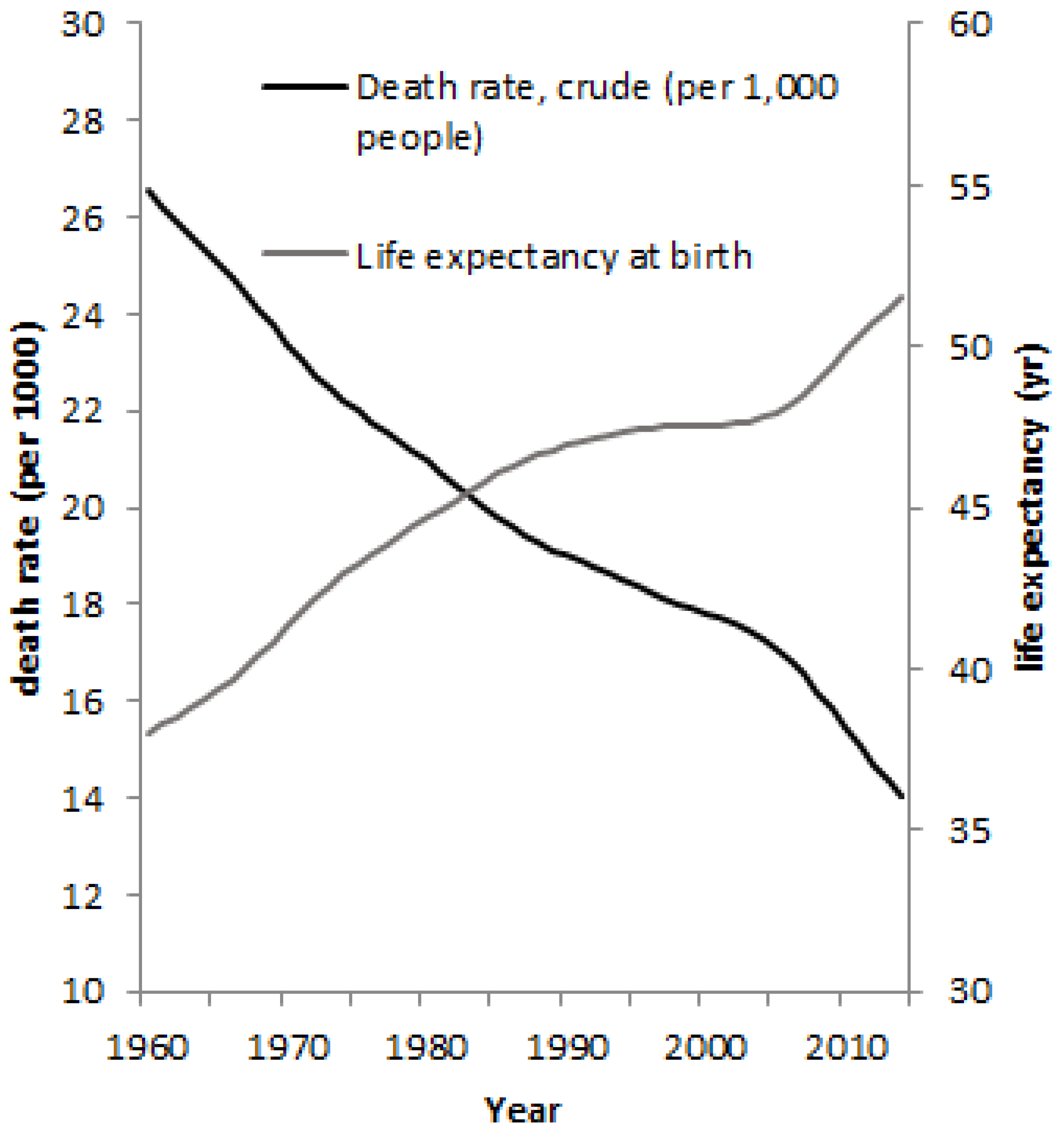
The demographic indicators in Figure 3 show the improvements in life chances over time that are compatible with food security and socio-economic growth since Independence. However, during the 1990s and early 2000s there is a slowing or cessation of improvement. This cessation, or even reversal, of improvement in life chances is even more obvious in sub-Saharan countries and has been commonly ascribed to the spread of the HIV infection (De Walque and Filmer 2013), suggesting that the cause is more complex than merely being conflict-related. There are therefore a range of factors at play in African society, some acting to add stress to society (u2, u4, u6, u7, and u10), while others will act to alleviate stresses (u1, u3, u5, u8, and u9). We will next investigate the roles these explanatory variables play in change in demographic indicators of death rate and life expectancy through NARX modelling.
4.2. The Identified Nonlinear Models
As the spread of HIV began in the central part of our timeseries, we have built two groups of models for y1 and y2 for each of our transect countries. One group uses explanatory variables u1,…,u9 over 1960–2010, with four years (2011–2014) for model testing, while the other splits the time period into two intervals, with the first period just using u1,…,u9 over 1960–1986, and three test years (1987–1989), and the second using all u1,…,u10 over 1990–2012, with two test years (2013–2014). The second split model gives the opportunity to examine the impact of HIV infection on the basic drivers of life chance changes. The five most important terms of each model of national death rates, or less if a particular model requires less terms, are shown in Supplementary Material in Table S2 for the N-S transect and Table S3 for the W-E transect, while Tables S4 and S5 respectively show these for life expectancy models.
5. Discussion
The discussion will examine the dominant terms in the N-S transect demographic models, and then move to the W-E transect models. General common and divergent trends will then be considered.
5.1. N-S Transect
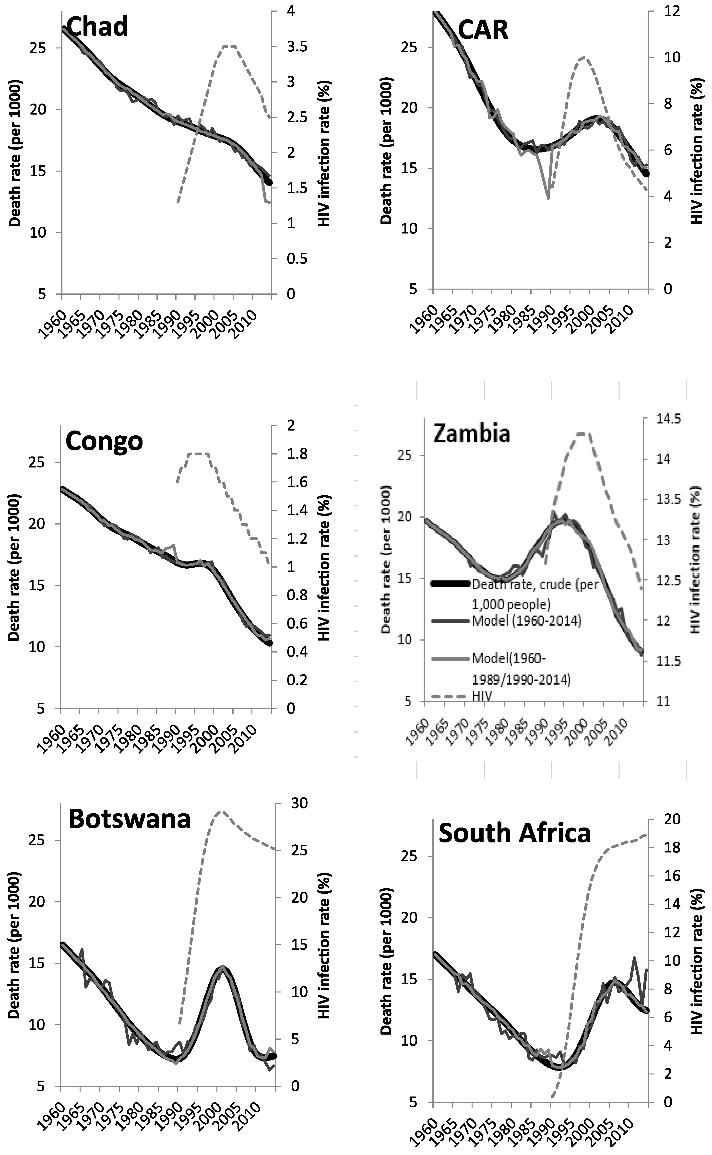
When considering the death rate (Table S2), it can be seen that the whole period models across most of the transect are dominated by food variables (particularly u5, but also u9), with water supply, u7 or u2, a secondary feature. This food dominance is strongest in the northern desert and central rain forest countries. Temperature plays no part in the models (except in the least significant term in the South African model), while the economic indicator of u3 plays a very minor role, at best, in any country. When the period is divided, and HIV, as u10, is included after 1989, food or water remain dominant factors in the death rate models in the first half of the period but u10 plays the major, or at least a secondary, role in all models. There is a strong correspondence between HIV and death rate increase, which is particularly notable from the Congo southwards (Figure 4). Note, however, that food or water variables remain very important in this latter period, with the HIV term being non-linearly linked to other variables (Table S2), as is consistent with Loevinsohn (2015). The only exception to this is in the Congo, where HIV is the leading, linear, term in the late period model, despite some evidence of conflict increasing infant mortality here (Lindskog 2016).
In 60% of the models, the first order term, which always has an ERR value well over 90%, is linear, while the model higher order terms are overwhelmingly non-linear (93 out of 100 terms). Every country in the N-S transect has at least 1 period, and in the case of the Congo all models, with one simple linear term being able to capture the death rate variability. Note, however, that only in around a half of such simple terms is the lag coefficient of the dominant explanatory variable just one year, while all leading order non-linear terms have longer lags. Thus, while most countries in the transect respond at some time to a stress linearly and quickly, most have death rates that respond in a more complex manner, and more slowly, to stress.
With regard to the life expectancy demographic variable for the N-S transect (Table S4), food-related variables are again dominant, being represented in 65% of the first order terms. However, neither water nor temperature terms play very much of a role in any models, while economic growth, u3, and the population growth rate, u4, are now the main secondary factors. The latter can also be seen as an economic-related factor, as population will likely grow more readily when health services, dependent on economic growth, are increasing. Interestingly, as many leading order terms are linear in life expectancy models as in those of the death rate models. This is true whether food or economic factors are dominant. Again, all countries have at least one model period where the dominant term has a factor with a one year lag, suggesting often rapid responses of life expectancy to stress (or more normally stress release, as such terms are positive in all bar one case). Nevertheless, the economic terms often have greater lags, reflecting the more cumulative nature of demographic change linked to economic growth.
5.2. W-E Transects
In considering the death rates across the W-E transect (Table S3), it is clear that food-related effects still dominant the leading order terms of the models. The major exception to this is in Niger, where economic-related variables are the leading terms. It is also noteworthy that in Mali, while food-related variables (u7 and u8) are involved in the whole period and early period models, the death rate is strongly and linearly driven by the HIV infection rate (u10), with a three-year lag. This is a shorter timescale than those reported for HIV patients in trials from the area (Morgan et al. 2002), but consistent with HIV not being reported by individuals until a health problem arises (Morgan et al. 1997). Only Mali displays a strong HIV link to death rates in this transect, however.
Amongst secondary effects, both temperature (u6) and water-related terms (u2 and u7) are present in most models, with these being stronger in the west of the transect than the east. As with the N-S transect, 60% of the leading order terms show strong linear relations between death rate and the appropriate variable (Table S3), although no country has linear leading order terms for all three model cases. In contrast to the N-S transect no country in the W-E transect suggests a fast, one-year, response to the leading term across all three cases, and in most cases the lags are several years duration.
With the life expectancy demographic variable (Table S5), the economic-related variables (u3 and u4) occur in leading order terms of all models across all countries, except Sudan. In the latter country, there was a change from population growth (u4) to food availability (u5) being the dominant, and linear, leading order term from the first half of the period to the second. This is likely to be related to the onset of the Second Civil War in Sudan in 1983 and drought conditions.
Linearity in the leading order model terms for life expectancy is even stronger than for the N-S transect, with ~75% of such terms being linear. Sudan shows linearity in all terms. This is also a fast response system, with just one-year lags for all model periods. Apart from Niger, other countries typically have longer lag periods.
5.3. Similarities and Contrasts between Transects
A strong relationship appears within many models, across both transects, between food supply and death rate, while environmental and economic effects are secondary, if present at all, in most models in most countries. While food-related terms are important, this dominance is less true of the life expectancy demographic variable, where economic-related variables also can play a significant role in model terms, particularly in the W-E, Sahel transect.
It is also noteworthy that there is a greater tendency for leading order terms, which always explain well over 90% of ERR, to be linear than to be non-linear for both the death rate and life expectancy. Linearity does not always mean the demographic system responds quickly to the dominant forcing term, as fewer than 40% of the leading order model terms have an element with a one-year lag. Longer lead times, of up to five years, are more common. HIV infection rates (u10) have played a role since 1990 in explaining the demographic change of sub-Saharan Africa. This extends throughout the N-S transect, from Chad south, but only Mali of the Sahelian transect, in addition to the common transect country of Chad, has u10 in a post-1989 model.
6. Conclusions
This paper has introduced a new approach to modelling societal stresses, represented here by the demographic variables of death rate and life expectancy, derived from the discipline of control engineering, which is also robust enough for forecasting purposes. It shows that quantitative relationships between variables representing these stresses and a mix of environmental, economic, and demographic variables are more complex than sometimes thought across Africa, and lead to relationships that support recent new ways of thinking about the complex interactions between society and the environment (Sen 2008; Allouche 2011; Butler 2014).
Political processes, colonial antecedents, conflict, and aspects of medical care like the prevalence of doctors and contraceptive policies are other factors that could be included in an analysis but have not been examined here. This is partly because data on these aspects are not readily included due to being subjective, such as political processes and colonial origins, or because data are patchy and imprecise (conflict) or do not extend across the whole period (many potential medical or birth control variables). Indeed, battle deaths as a measure of conflict, available through the World Bank database but derived from Lacina and Gelditsch (2005), were included in a pilot analysis for Chad, but the quality of the data meant that this variable was dropped from our full analysis. Nevertheless, our study suggests food production is an important factor leading to societal stresses across much of Africa, although not always in a direct way, and that direct temperature or economic effects may not be as important as sometimes claimed. For many countries, and time periods, the connection between food supplies and death rate is not as fast as might be expected—the immediacy of a link that an event such as drought-driven crop failure would imply is largely restricted to the countries of the Sahel (Mauritania, Chad, and Sudan). Thus, while our analysis supports a need for rapid international response to food emergencies across the extended Sahel region, a longer-term perspective on managing food availability may be more appropriate elsewhere.
This study has taken a continental-scale approach to the modelling problem to avoid the greater variability of causal relationships at local level (Allouche 2011). This also removes the local impact of colonialism, although it is worth noting that all our modelled countries had a colonial past providing some measure of a common background. It has shown that there are large-scale relationships between demographic variables and environmental and societal change. Nevertheless, the best fitting models for individual countries are quite variable. Large-scale analysis reveals general trends and relations, but this suggests that a detailed understanding of a particular country’s development, and a forecast of change, needs more local analysis. Detailed policy decisions for specific countries on how to manage the interplay between environmental, socio-economic, and demographic processes are therefore recommended to be based on local studies.
Supplementary Materials
The following are available online at www.mdpi.com/2076-0760/6/4/122/s1.
Acknowledgments
This work was assisted by support from the EPSRC Platform grant EP/H00453X/1. We gratefully acknowledge the broadening of background ideas provided by a reading of an earlier version by Peter Jackson.
Author Contribution
Bigg proposed the project, provided the data and wrote much of the text, while Wei developed the NARX model and wrote the method section of the text.
Conflicts of Interest
The authors declare no conflict of interest. The funding sponsor had no role in the design of the study; in the collection, analyses or interpretation of data; in the writing of the manuscript, and in the decision to publish the results.
References
- Akanyeti, Otar, Ulrich Nehmzow, and Steve A. Billings. 2008. Robot training using system identification. Robotics and Autonomous Systems 56: 1027–41. [Google Scholar] [CrossRef]
- Allouche, Jeremy. 2011. The sustainability and resilience of global water and food systems: Political analysis of the interplay between security, resource scarcity, political systems and global trade. Food Policy 36: S3–8. [Google Scholar] [CrossRef]
- Balikhin, Michael A., Richard J. Boynton, Simon N. Walker, J. E. Borovsky, Steve A. Billings, and Hua-liang Wei. 2011. Using the NARMAX approach to model the evolution of energetic electrons fluxes at geostationary orbit. Geophysical Research Letters 38: L18105. [Google Scholar] [CrossRef]
- Bernauer, Thomas, Tobias Böhmelt, and Valli Koubi. 2012. Environmental changes and violent conflict. Environmental Research Letters, 7. [Google Scholar] [CrossRef] [Green Version]
- Bigg, Grant R., Hua-Liang Wei, David J. Wilton, Yifan Zhao, Steve A. Billings, Edward Hanna, and Visakan Kadirkamanathan. 2014. A century of variation in the dependence of Greenland iceberg calving on ice sheet surface mass balance and regional climate change. Proceedings of the Royal Society Series A 470. [Google Scholar] [CrossRef] [PubMed]
- Billings, Steve A. 2013. Non-Linear System Identification: NARMAX Methods in the Time, Frequency, and Spatio-Temporal Domains. London: Wiley. [Google Scholar]
- Billings, Catherine G., Hua-Liang Wei, Patrick Thomas, S. J. Linnane, and B. D. M. HopeGill. 2013. The prediction of in-flight hypoxaemia using non-linear equations. Respiratory Medicine 107: 841–847. [Google Scholar] [CrossRef] [PubMed]
- Billings, Steve A., and Hua-Liang Wei. 2005. The wavelet-NARMAX representation: A hybrid model structure combining polynomial models with multiresolution wavelet decompositions. International Journal of Systems Science 36: 137–52. [Google Scholar] [CrossRef]
- Blouin, Max, and Stephane Pallage. 2016. Warlords, famine and food aid: Who fights, who starves? European Journal of Political Economy 45: 18–38. [Google Scholar] [CrossRef]
- Buhaug, Halvard. 2010. Climate not to blame for African civil wars. Proceedings of the National Academy of Sciences USA 107: 16477–82. [Google Scholar] [CrossRef] [PubMed]
- Burkart, Katrin, Mohammed Mobarrak Hossain Khan, Alexandra Schneider, Susanne Breitner, Marcel Langner, Alexander Kraemer, and Wilfried Endlicher. 2014. The effect of season and meteorology on human mortality in tropical climates: A systematic review. Transactions of the Royal Society of Tropical Medicine and Hygiene 108: 393–401. [Google Scholar] [CrossRef] [PubMed]
- Burke, Marshall B., Edward Miguel, Shanker Satyanath, John A. Dykema, and David B. Lobell. 2009. Warming increases the risk of civil war in Africa. Proceedings of the National Academy of Sciences USA 106: 20670–74. [Google Scholar] [CrossRef] [PubMed]
- Butler, Colin D. 2014. Famine, hunger, society and climate change. In Climate Change and Global Health. Edited by Colin D. Butler. Oxford: Centre for Agriculture and Biosciences International, pp. 124–34. [Google Scholar]
- Canning, David. 2011. The causes and consequences of demographic transition. Population Studies 65: 353–61. [Google Scholar] [CrossRef] [PubMed]
- Chen, Sheng, and Steve A. Billings. 1989. Representation of non-linear systems: The NARMAX model. International Journal of Control 49: 1013–32. [Google Scholar] [CrossRef]
- Chen, Sheng, Steve A. Billings, Colin F. N. Cowan, and Peter M. Grant. 1990. Practical identification of NARMAX models using radial basis functions. International Journal of Control 52: 1327–50. [Google Scholar] [CrossRef]
- Chiras, Neopbytos, Ceri Evans, and David Rees. 2001. Nonlinear gas turbine modeling using NARMAX structures. IEEE Transactions on Instrumentation and Measurement 50: 893–98. [Google Scholar] [CrossRef]
- De Walque, Damien, and Deon Filmer. 2013. Trends and socioeconomic gradients in adult mortality around the developing world. Population and Development Review 39: 1–29. [Google Scholar] [CrossRef]
- Dong, Weihua, Zhao Liu, Hua Liao, Qiuhong Tang, and Xian’en Li. 2015. New climate and socio-economic scenarios for assessing global human health challenges due to heat risk. Climate Change 130: 505–18. [Google Scholar] [CrossRef]
- Eastwood, Robert, and Michael Lipton. 2011. Demographic transition in sub-Saharan Africa: How big will the economic divide be? Population Studies 65: 9–35. [Google Scholar] [CrossRef] [PubMed]
- Evenson, Robert E., and Douglas Gollin. 2003. Assessing the impact of the Green Revolution, 1960–2000. Science 300: 758–62. [Google Scholar] [CrossRef] [PubMed]
- Hartmann, Dennis L., Albert M. G. Klein Tank, Matilde Rusticucci, Lisa V. Alexander, Stefan Brömmimann, Yassine Charabi, Frank J. Dentener, Edward J. Dlugokencky, David R. Easterling, Alexey Kaplan, and et al. 2013. Observations: atmosphere and surface. In Climate Change 2013: The Physical Science Basis. Edited by Thomas F. Stocker, Dahe Qin, Gian-Kasper Plattner, Melinda M.B. Tigonor, Simon K. Allen, Judith Boschung, Alexander Nauels, Yu Xia, Vincent Bex and Pauline M. Midgley. Cambridge: Cambridge University Press, pp. 159–254. [Google Scholar]
- Jeuland, Marc A., David E. Fuente, Semra Ozdemir, Maura C. Allaire, and Dale Whittington. 2013. The long-term dynamics of mortality benefits from improved water and sanitation in less developed countries. PLoS ONE 8: e74804. [Google Scholar] [CrossRef] [PubMed]
- Lacina, Bethany, and Nils P. Gleditsch. 2005. Monitoring trends in global combat: A new dataset of battle deaths. European Journal of Population 21: 145–66. [Google Scholar] [CrossRef]
- Leontaritis, I. J., and Steve A. Billings. 1985a. Input–output parametric models for non-linear systems—Part I: Deterministic non-linear systems. International Journal of Control 41: 303–28. [Google Scholar] [CrossRef]
- Leontaritis, I. J., and Steve A. Billings. 1985b. Input–output parametric models for non-linear systems—Part II: Stochastic non-linear systems. International Journal of Control 41: 329–44. [Google Scholar] [CrossRef]
- Lindskog, Elina Elveborg. 2016. The effect of war on infant mortality in the Democratic Republic of Congo. BMC Public Health 16: 1059. [Google Scholar] [CrossRef] [PubMed]
- Loevinsohn, Michael. 2015. The 2001–03 famine and the dynamics of HIV in Malawi: A natural experiment. PLoS ONE 10: e0135108. [Google Scholar] [CrossRef] [PubMed]
- Marshall, Abigail M., Grant R. Bigg, Sonja M. van Leeuwen, John K. Pinnegar, Hua-Liang Wei, Thomas J. Webb, and Julia L. Blanchard. 2016. Quantifying heterogeneous responses of fish community size structure using novel combined statistical techniques. Global Change Biology 22: 1755–68. [Google Scholar] [CrossRef] [PubMed]
- Mathers, Colin D., Ties Boerma, and Doris Ma Fat. 2009. Global and regional causes of death. British Medical Bulletin 92: 7–32. [Google Scholar] [CrossRef] [PubMed]
- Morgan, Dilys, Gillian H. Maude, Samuel S. Malamba, Martin J. Okongo, Hans-Ulrich Wagner, Daan W. Mulder, and James A. Whitworth. 1997. HIV-1 disease progression and AIDS-defining disorders in rural Uganda. Lancet 350: 245–50. [Google Scholar] [CrossRef]
- Morgan, Dilys, Cedric Mahe, Billy Mayanja, Martin J. Okongo, Rosemary Lubega, and James A. G. Whitworth. 2002. HIV-1 infection in rural Africa: is there a difference in median time to AIDS and survival with that in industrialized countries? AIDS 16: 597–603. [Google Scholar] [CrossRef] [PubMed]
- Nelles, Oliver. 2001. Nonlinear System Identification. Berlin: Springer. [Google Scholar]
- Nicholson, Sharon E. 2001. Climatic and environmental change in Africa during the last two centuries. Climate Research 17: 123–44. [Google Scholar] [CrossRef]
- OECD. 2013. Life Expectancy at Birth, in Health at a Glance 2013 OECD Indicators. Paris: OECD Publishing, Available online: http://dx.doi.org/10.1787/health_glance-2013-5-en (accessed on 13 October 2017).
- Salam, Asharaf Abdul, Ibrahim Elsegaey, Rshood Khraif, Abdullah AlMutairi, and Ali Aldosari. 2015. Components and public health impact of population growth in the Arab World. PLoS ONE 10: e0124944. [Google Scholar] [CrossRef] [PubMed]
- Sarrigiannis, Ptolemaios G., Yifan Zhao, Hua-Liang Wei, Steve A. Billings, Jayne Fotheringham, and Marios Hadjivassiliou. 2014. Quantitative EEG analysis using error reduction ratio-causality test: Validation on simulated and real EEG data. Clinical Neurophysiology 125: 32–46. [Google Scholar] [CrossRef] [PubMed]
- Schönfeldt, Hettie C., and Nicolette G. Hall. 2012. Dietary protein quality and malnutrition in Africa. British Journal of Nutrition 108: S69–76. [Google Scholar] [CrossRef] [PubMed]
- Sen, Amartya. 2008. Violence, identity and poverty. Journal of Peace Research 45: 5–15. [Google Scholar] [CrossRef]
- Song, Zhuoyi, Marten Postma, Steve A. Billings, Daniel Coca, Roger C. Hardie, and Mikko Juusola. 2012. Stochastic, Adaptive Sampling of Information by Microvilli in Fly Photoreceptors. Current Biology 22: 1371–80. [Google Scholar] [CrossRef] [PubMed]
- Theisen, Ole M., Nils P. Gleditsch, and Halvard Buhaug. 2013. Is climate change a driver of armed conflict? Climatic Change 117: 613–25. [Google Scholar] [CrossRef]
- Wandiga, Shem O., Maggie Opondo, Daniel Olago, Andrew Githeko, Faith Githui, Michael Marshall, Tim Downs, Alfred Opere, Christopher Oludhe, Gilbert O. Ouma, and et al. 2010. Vulnerability to epidemic malaria in the highlands of Lake Victoria basin: The role of climate change/variability, hydrology and socio-economic factors. Climatic Change 99: 473–97. [Google Scholar] [CrossRef]
- Wei, Hua-Liang, and Steve A. Billings. 2008. Model structure selection using an integrated forward orthogonal search algorithm assisted by squared correlation and mutual information, International Journal of Modelling. Identification and Control 3: 341–56. [Google Scholar]
- Wei, Hua-Liang, Steve A. Billings, and Michael Balikhin. 2004a. Prediction of the Dst index using multiresolution wavelet models. Journal of Geophysical Research—Atmospheres 109: A07212. [Google Scholar] [CrossRef]
- Wei, Hua-Liang, Steve A. Billings, and Jianhua Liu. 2004b. Term and variable selection for nonlinear system identification. International Journal of Control 77: 86–110. [Google Scholar] [CrossRef]
- Wei, Hua-Liang, Steve A. Billings, and Michael A. Balikhin. 2006. Wavelet based non-parametric NARX models for nonlinear input-output system identification. International Journal of Systems Science 37: 1089–96. [Google Scholar] [CrossRef]
- Wei, Hua-Liang, Ding-Qiu Zhu, Steve A. Billings, and Michael A. Balikhin. 2007. Forecasting the geomagnetic activity of the Dst index using multiscale radial basis function networks. Advances in Space Research 40: 1863–70. [Google Scholar] [CrossRef]
- Wei, Hua-Liang, Steve A. Billings, Yifan Zhao, and Lingzhong Guo. 2010. An adaptive wavelet neural network for spatio-temporal system identification. Neural Networks 23: 1286–99. [Google Scholar] [CrossRef] [PubMed]
- Yaduma, Natina, Mika Kortelainen, and Ada Wossink. 2013. Estimating mortality and economic costs of particulate air pollution in developing countries: The case of Nigeria. Environmental & Resource Economics 54: 361–87. [Google Scholar]
- Zaman, Khalid, Aqeel Ahmad, Tengku Adeline Adura Tengku Hamzah, and Mariney Mohd Yusoff. 2016. Environmental factors affecting health indicators in sub-Saharan African countries: Health is wealth. Social Indicators Research 129: 215–28. [Google Scholar] [CrossRef]
- Zhang, David D., Peter Brecke, Harry F. Lee, Yuan-Qing He, and Jane Zhang. 2007. Global climate change, war, and population decline in recent human history. Proceedings of the National Academy of Sciences USA 104: 19214–19. [Google Scholar] [CrossRef] [PubMed]
- Zhao, Yifan, Steve A. Billings, Hua-Liang Wei, and Ptolemaios G. Sarrigiannis. 2012. Tracking time varying causality and directionality of information flow using an error reduction test with applications to electroencephalography data. Physics Review E 86: 1–11. [Google Scholar] [CrossRef] [PubMed]
- Zhao, Yifan, Grant R. Bigg, Stephen A. Billings, Edward Hanna, Andrew J. Sole, Hua-Liang Wei, Visakan Kadirkamanathan, and David J. Wilton. 2016. Inferring the variation of climatic and glaciological contributions to West Greenland iceberg discharge in the twentieth century. Cold Regions Science and Technology 121: 167–78. [Google Scholar] [CrossRef]
Figure 1.
Map of Africa showing the nations modelled in the north-south (white) and west-east (light grey) transects. Note that Chad (dark grey) is in both transects. The new nation of South Sudan is outlined within the most eastern nation of Sudan.
Figure 1.
Map of Africa showing the nations modelled in the north-south (white) and west-east (light grey) transects. Note that Chad (dark grey) is in both transects. The new nation of South Sudan is outlined within the most eastern nation of Sudan.
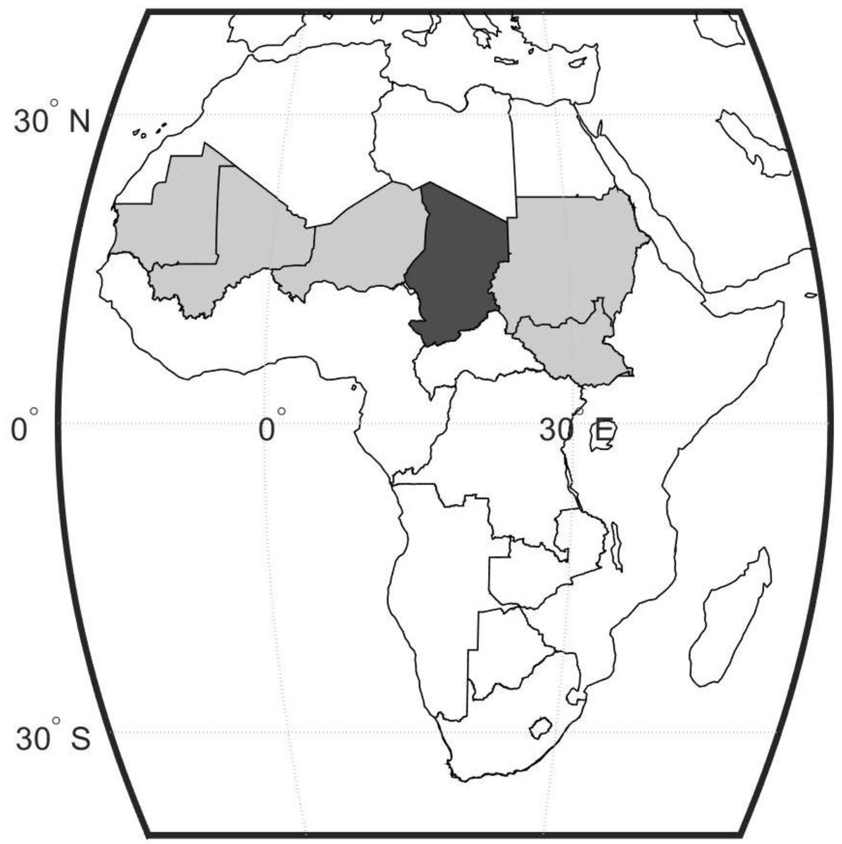
Figure 2.
Timeseries of 9 explanatory variables for Chad over 1960–2014. The left panel is for u1, u4, u5, and u6 while the right panel is for u2, u3, u7, u8, and u9. See Table 1 for the source of data for the individual variables. The HIV variable is shown in Figure 4. For information, the timings of key political events are: 1967—beginning of civil war; 1978—Libyan intervention; 1988—expulsion of Libyan troops; 1990—Dèby takes control; 2007—start of Sudanese war and second civil war; 2010—end of wars.
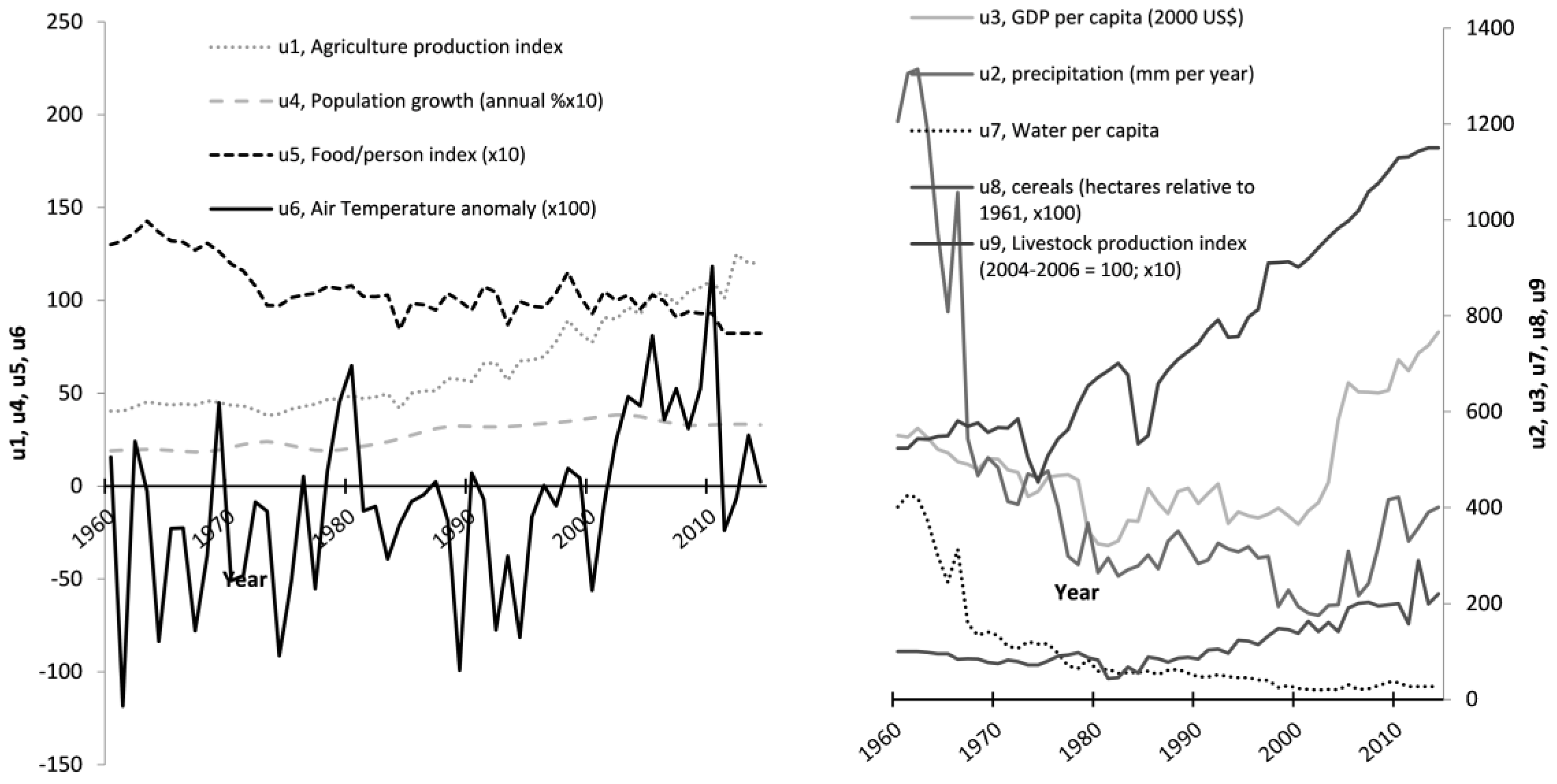
Figure 3.
Life expectancy and death rate in Chad over 1960–2014. See Table 1 for source of data.
Figure 3.
Life expectancy and death rate in Chad over 1960–2014. See Table 1 for source of data.

Figure 4.
Panels show the death rate of the N-S transect countries (bold; except Libya), with the full period model (light grey), and the combined early and late period model (dark grey) fits. The HIV infection rate is dashed. See Table 1 for the sources of the data.
Figure 4.
Panels show the death rate of the N-S transect countries (bold; except Libya), with the full period model (light grey), and the combined early and late period model (dark grey) fits. The HIV infection rate is dashed. See Table 1 for the sources of the data.


Table 1.
Variables used in this study.
| Variable | Description |
|---|---|
| u1 (explanatory)1 | Agricultural production index (1999–2001 = 100) |
| u2 (explanatory)2 | Average precipitation (mm·yr−1) |
| u3 (explanatory)3 | GDP per capita (constant 2000 US$) |
| u4 (explanatory)4 | Population growth (annual %) |
| u5 (explanatory)5 | Food/person index |
| u6 (explanatory)2 | Average annual air temperature anomaly (°C) |
| u7 (explanatory)5 | Water per capita |
| u8 (explanatory)3 | Land under cereal production (hectares relative to 1961) |
| u9 (explanatory)3 | Livestock production index (2005–2006 = 100) |
| u10 (explanatory)3 | HIV infection rate (from 1990; % population aged 15–49) |
| y1 (response)3 | Death rate, crude (per 1000 people) |
| y2 (response)3 | Life expectancy at birth (years) |
Note: Data sources (see text for details): 1 FAO; 2 NCEP climate data; 3 World Bank; 4 UN Population Division; 5 our calculation, using two different sources.
Table 2.
Regions used for climate variable calculations for modelled countries (bold—N-S transect; italics—W-E transect).
Table 2.
Regions used for climate variable calculations for modelled countries (bold—N-S transect; italics—W-E transect).
| Country | Latitude Band | Longitude Band |
|---|---|---|
| Libya | 20–33° N | 10–25° E |
| Chad | 8.5–24° N | 13–24° E |
| Central African Republic | 3–10° N | 15–27° E |
| Democratic Republic of Congo | 12° S–5° N | 13–30° E |
| Zambia | 9–18° S | 22–33° E |
| Botswana | 18–26° S | 20–29° E |
| South Africa | 22–34° S | 17–33° E |
| Mauritania | 16–26° N | 16–6° W |
| Mali | 10–24° N | 12° W–4° E |
| Niger | 13–23° N | 0–15° E |
| Sudan | 10–22° N | 24–38° E |
© 2017 by the authors. Licensee MDPI, Basel, Switzerland. This article is an open access article distributed under the terms and conditions of the Creative Commons Attribution (CC BY) license (http://creativecommons.org/licenses/by/4.0/).
Share and Cite
MDPI and ACS Style
Wei, H.; Bigg, G.R. The Dominance of Food Supply in Changing Demographic Factors across Africa: A Model Using a Systems Identification Approach. Soc. Sci. 2017, 6, 122. https://doi.org/10.3390/socsci6040122
AMA Style
Wei H, Bigg GR. The Dominance of Food Supply in Changing Demographic Factors across Africa: A Model Using a Systems Identification Approach. Social Sciences. 2017; 6(4):122. https://doi.org/10.3390/socsci6040122
Chicago/Turabian StyleWei, Hualiang, and Grant R. Bigg. 2017. "The Dominance of Food Supply in Changing Demographic Factors across Africa: A Model Using a Systems Identification Approach" Social Sciences 6, no. 4: 122. https://doi.org/10.3390/socsci6040122
Note that from the first issue of 2016, this journal uses article numbers instead of page numbers. See further details here.